1. INTRODUCTION
An engineered system is defined as an assemblage of subsystems, hardware/software components, and people designed to perform a set of tasks to satisfy specified functional requirements and constraints (Suh, Reference Suh1998). The traditional approach for designing an engineered system is to establish a predefined set of requirements based on market studies and best estimate extrapolations of the current state, and then find the optimal design to satisfy the requirements (Siddiqi & de Weck, Reference Siddiqi and de Weck2008). Chen et al. (Reference Chen, Hoyle and Wassenaar2013a , Reference Chen, Hoyle and Wassenaar2013b , Reference Chen, Hoyle and Wassenaar2013c , Reference Chen, Hoyle and Wassenaar2013d ) developed the decision-based design approach to design engineered system; the authors apply optimization and utility theory to select the best design. However, these approaches are inadequate to respond to changes in initial requirements or changes in operating conditions. This can lead to technical or economic failure if the system is faced with significantly different conditions than the ones predicted.
The economic troubles of the IRIDIUM (Pratt et al., Reference Pratt, Raines, Fossa and Temple1999) and GLOBALSTAR (Lutz et al., Reference Lutz, Werner and Jahn2012) ventures illustrate the significance of resiliency of engineered systems in responding to potential uncertainties in demand. Both of these satellite communication systems in low earth orbit (LEO) forecasted a large number of customers based on a certain type of service (telephony along with fax, messaging, etc.). Although both systems were successful technically, they failed economically due to market changes that had taken place between the time of conceptual design and the time they became operational, resulting in losses of roughly $4 and $3.5 billion, respectively. The proximate cause of these failures is that prior forecasts and expectations were confounded; specifically, the market for wireless telephony went to ground-based competitors that arose between the system conception in 1990, and the launch of the ill-fated communication satellites starting in 1998. The satellite systems were too inflexible to be easily downsized or switched to a different type of service or coverage. Attention to such cases illustrates the coupling of design, performance, and economics, and motivates engineers to investigate ways of making engineering systems resilient to uncertainties in future states. Keshavarzi et al. (Reference Keshavarzi, McIntire and Hoyle2015) have introduced a dynamic design approach that enables complex engineering systems to overcome such uncertainties in the operational phase.
The main goal of this paper is to present an approach for system design to manage the uncertainty in a state of interest (SoI) throughout the life cycle of the system. The SoI in this work is the state of an uncertain internal or external condition that directly influences the success of the system throughout its life cycle. The uncertain condition is usually rooted in the operating environment of the system. Examples of a SoI are the state of health of an aerospace or automotive vehicle (internal state), the demand for its goods or services (external state), or the state of technology for system components (external state). These example SoIs share a common attribute in that they are highly related to the success of a given system, yet they can only be forecasted with considerable uncertainty. The current state of such conditions often can only be inferred through indirect measurement, for example, aggregating sensor data to estimate the state of health of an aerospace vehicle, or counting the number of users for data services to estimate the actual service demand. Viewing system design as an optimization problem, the SoI will appear in the objective or constraints, and thus has a quantifiable impact on the values of design variables and hence system performance.
The material of the paper is organized as follows: Section 2 proposes a clear and consistent definition of flexibility of a design as a tool to enable resilient design, while carefully disentangling it from discussions on flexibility in the design process. Section 3 illustrates the different types of uncertainty in engineered systems with a focus on time-resolved uncertainties. Section 4 formalizes the design decision-making process, and Section 5 provides the Kalman filter approach to making design selections. Section 6 provides a case study of a space-borne system design, to illustrate the application of the Kalman filter method. Section 7 provides summary and conclusion.
2. RESILIENT DESIGN
Developing resilient engineered systems is of increasing interest in the design community. Resilient design enables engineering systems to recover from uncertain event occurrences (Hollnagel et al. Reference Hollnagel, Woods and Leveson2007). A resilient system is one that maintains state awareness and an accepted level of operational normalcy in response to disturbances, including threats of an unexpected and malicious nature (Rieger, Reference Rieger2009). Flexibility is an effective means to embed resiliency into an engineering system design; however, flexibility is a word rich in ambiguity. While it is increasingly being used in various fields, few attempts have been made to formally define, quantify, and propose ways of achieving flexibility. Saleh (Reference Saleh2001) investigated 50 definitions of flexibility in different fields, and proposed the clear definition of flexibility as the ability of a system “to respond to changes in initial requirements and objectives, after it has been fielded, in a timely and cost-effective way.” This definition places the emphasis on change after the system starts operating. As pointed out in Lamasourre et al. (Reference Lamassoure, Saleh and Hastings2002), flexibility is necessary as a response to uncertainty in use. If we knew exactly how a system would be used for its design lifetime and beyond, then it would be designed into the system from the beginning (Saleh et al., Reference Saleh, Lamassoure and Hastings2002). Therefore, flexible systems are understood to be those systems that can be changed or adapted in order to meet new or changed requirements.
The literature on flexibility in engineering design addresses two distinct problems: the flexibility of the design process (Suh et al., Reference Suh, de Weck, Kim and Chang2007) and the flexibility of the design itself (not the process through which the product or system is designed). This distinction between the flexibility of the process and the flexibility of the design is often forgotten in the literature, and it adds to the confusion in this emerging field (Saleh et al., Reference Saleh, Mark and Jordan2009). Flexibility is a key property that should be embedded in the designs of engineered systems to enable resilient designs, particularly as they are being designed to cope with time-resolved uncertainties (Mark, Reference Mark2005). In the following sections, descriptions of the different types of uncertainty, and their relation to resilient design, are presented.
3. UNCERTAINTY IN ENGINEERING SYSTEMS
Uncertainty is the inability to specify something with precision (Antonsson & Otto, Reference Antonsson and Otto1995), and is the key driver for the need for resilient designs. Uncertainty influences designs, decisions, and behaviors in a variety of fields, from economics to engineering; reducing uncertainty is costly in both time and resources (Helton, Reference Helton1997). While there can be many classifications of uncertainty, for the purpose of this work, uncertainty in engineered systems may be classified as statistical and time resolved (Thunnissen, Reference Thunnissen2005).
3.1. Statistical uncertainty
Statistic uncertainty is inherent variation associated with a physical system or environment under consideration (DeLaurentis & Mavris, Reference DeLaurentis and Mavris2000). Statistical uncertainty goes by many names: aleatory uncertainty, variability, irreducible uncertainty, stochastic uncertainty, noise, risk, type “A” uncertainty, and de re (Igusa et al., Reference Igusa, Buonopane and Ellingwood2002). Statistical uncertainties can be differentiated from time-resolved uncertainties by their representation as quantities that can take on values in a known range or distribution. The mathematical representation most commonly used for statistical uncertainty is a probability distribution function.
3.2. Time-resolved (epistemic) uncertainty
Time-resolved uncertainty refers to the types of uncertainties that will be resolved or reduced over the system's life cycle. These are traditionally classified as epistemic uncertainties. The key feature of epistemic uncertainty is that the fundamental cause is incomplete information or incomplete knowledge of some characteristic of the system or the environment. Quantification of the impacts of time-resolved, or epistemic, uncertainty is inherently difficult, because most of the existing stochastic tools rely on the specification of probability distributions, and thus do not readily apply to epistemic uncertainty (Chen et al., Reference Chen, Park and Xiu2013). Epistemic uncertainty also goes by these names: reducible uncertainty, subjective uncertainty, model form uncertainty, state of knowledge, type “B” uncertainty, and de dicto (Bae et al., Reference Bae, Grandhi and Canfield2004). A key feature of time-resolved uncertainties is that the resolution (or reduction) of the uncertainty provides an opportunity for updated design decision making, if flexibility has been provided in the design. As an example of this process, future demand for a system is an epistemic uncertain variable as sudden changes in the future may occur due to the introduction of a new technology to the market, changes in government policy, or changes in customers’ interests (Carvalho & Puterman, Reference Carvalho and Puterman2004). Future changes in demand, including changes in the type of demand or the number of users, are unknown when a system is being designed; however, when demand is observed, modifications can be made in response to the state of demand (i.e., the SoI).
Whereas much research has gone into quantifying aleatory uncertainty within the probabilistic framework (Oberkampf et al., Reference Oberkampf, Helton and Sentz2001), few approaches have been proposed as the most appropriate mathematical representation for epistemic uncertainty, as well as the accompanying decision-making methodology as the uncertainty is resolved. Possibility theory, first introduced by Zadeh (Reference Zadeh1965), has been applied in many areas to model epistemic uncertainty (Youn et al., Reference Youn, Choi, Du and Gorsich2007). Structural design problems with fuzzy variables were investigated by Wood et al. (Reference Wood, Otto and Antonsson1992), Antonsson and Otto (Reference Antonsson, Otto, Dubois, Prade and Yager1997), and Penmetsa and Grandhi (Reference Penmetsa and Grandhi2002). This approach can be used, but does not directly address the time-related aspect of the uncertainty. Bae et al. (2007) applied evidence theory, developed by Shafer (Reference Shafer1976), to quantify uncertainty when both kinds of uncertainties are presented in a system. Hofer et al. (Reference Hofer, Kloos, Krzykacz-Hausmann, Peschke and Woltereck2002) proposed using possibility theory to quantify epistemic uncertainties for robust and/or reliable design. Bayesian approaches to epistemic uncertainty have been investigated, for example, in Aughenbaugh and Paredis (Reference Aughenbaugh and Paredis2006), in which Bayesian methods are used to quantify uncertainty in engineering design. Herzig and Paredis (Reference Herzig and Paredis2014) applied a Bayesian method for validation and verification of models for engineering design. Bayesian approaches have the benefit of providing a means for both quantifying uncertainties at a given time and updating those “beliefs” as “evidence” becomes available. The Bayesian approach has been shown to be effective for quantifying time-resolved uncertainties; however, the approach must be extended for use in forecasting future states of interest. In addition, appropriate prior distributions must be employed, particularly when evidence is low.
When considering the role of epistemic uncertainty in the resilient design context, there currently is no consensus on the preferred approach to quantifying epistemic uncertainty in the literature, particularly when the entire life cycle of the product is considered (Dai et al. Reference Dai, Scott and Mourelatos2003). Further, there is no approach available to leverage the resolution of uncertainty to enable the design to be optimized in the new, lower uncertainty state. Much work has been dedicated to robustness, which refers to the ability to tolerate perturbations that might affect the system's functional body. Robustness is usually defined as “the ability of a system to resist change without adapting its initial stable configuration” (Fowlkes & Creveling, Reference Fowlkes and Creveling1995). Robustness, however, does not address recovery of the system; recovery is a feature of a resilient system. The main concern of this paper is to use resilient design to manage the epistemic uncertainty when the system design is flexible.
In this work, we apply the Kalman filter approach to forecast a future SoI, when a source of epistemic uncertainty occurs. Then based upon this modeled state, the optimal change in the design of the system will be achieved to respond to the new state. This resilient design method is applicable to systems when the ability to change is embedded in the system design.
4. DESIGNS AND STATES OF INTEREST
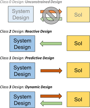
Before developing a design theory to accommodate time-resolved uncertainties, it is necessary to specify the relationship between the design and SoI. In general, we propose that four relationships between the design and SoI can occur in the design process, as shown in Figure 1 and described in this section as Class 0–4 design problems.
-
Class 0–Unconstrained design: In this class of design problem, the system design does not influence the SoI, and the SoI has no influence upon the optimal system design. An example is the design of automobile cup holder and the state of health of the automobile engine, which do not have any discernible relationship. This class is not explored further in this research, because there is no relationship to model.
-
Class 1–Predictive design: In this class, the system design influences the SoI; however, the SoI does not influence the design selection. An example is the design of an automobile exterior and the state of consumer preferences for the vehicle in a stable market. In this example, it is assumed that preferences (i.e., the SoI) for vehicle designs are stable, but that we can make a vehicle more (or less) preferred by changing its design. Design decisions for Class 1 designs have been modeled extensively using techniques such as generalized linear models or discrete choice analysis (e.g., Chen et al., Reference Chen, Hoyle and Wassenaar2013a ) to model the SoI as a function of independent design variables.
-
Class (2)–Reactive design: In this class, the future SoI has an influence upon the system design selection; however, the design does not influence the SoI. An example is the design of a power grid, which must be expanded and reconfigured based upon increasing state of demand due to population growth (i.e., an external source of change). In this example, it is assumed that changing the power grid design cannot drive demand, but that changes in demand (i.e., the SoI) drive changes to the grid design. Class 2 design has been studied primarily from the design for reconfigurability/flexibility standpoint, to provide necessary flexibility in the design to modify the system as needed over time (e.g., de Weck et al., Reference de Weck, Scialom and Siddiqi2008).
-
Class 3–Dynamic design: In this class, the system design influences the SoI, and the SoI influences the design selection. The future SoI is a function of the current state as well as the selected design. An example is the design of a smart phone and the state of consumer preferences for smart phones. In this example, at a given time period, preferences may be relatively stable, and this class of design may be similar to the Class 1 design in which the design may be altered to make the smart phone more (or less) preferred. Over time, however, preferences may be changing (e.g., size, shape, and weight preferences, need for apps), and the design may be altered to respond to these SoI changes, similar to Class 2 design. Another example is design for system health management, where one could make component redesigns to improve the system health in times when system health is stable, while also making redesigns to respond to changes in system health.
Classification of relationship between system design and state of interest.

The Class 3 design case is the case that represents the type of resilient design of interest in this research, and will be the focus of methodology development of the next section.
5. DYNAMIC DESIGN METHODOLOGY FOR RESILIENT DESIGN
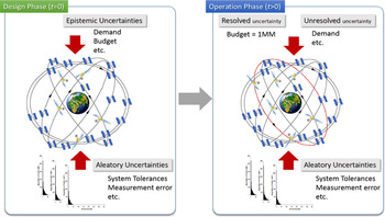
The traditional method of designing an engineered system is to design for a predefined set of requirements. It is based on a forecast of system needs, such as the expected number of users, available technology, or a given system health expectation. This can lead to technical or economic failure if the actual conditions or requirements are significantly different than those predicted (Siddiqi & de Weck, Reference Siddiqi and de Weck2008). As an example of system design challenges, Figure 2 illustrates a typical system design problem in which both aleatory and epistemic uncertainties are present in the design phase. While it is assumed that the aleatory uncertainties remain for the life of the system, epistemic uncertainties, such as operating budgets, demand for the system, or operating environments, may be resolved throughout the life of the system.
Design updating in the face of epistemic uncertainties.

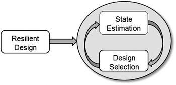
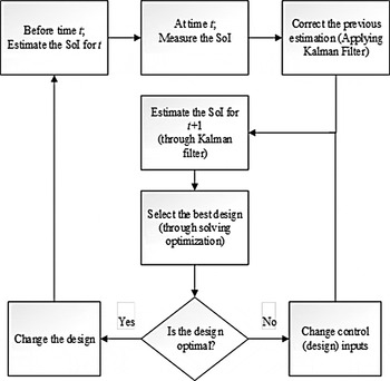
In this section, we present an approach to ensure the design is resilient to changes in the operating state as uncertainties are resolved. The key element in our approach is to use the Kalman filter to compute a best estimate of the future SoI, and then subsequently update the system design to meet this forecasted future state(s). A generalized framework of our approach is proposed in Figure 3. In this framework for an operating resilient system, the Kalman filter is utilized to estimate the SoI (Section 4.1). Optimization is then employed to determine how to update the design to best fit the forecasted operational environment (Section 4.2).
A generalized framework of the resilient design approach.

5.1. Kalman filter
In Reference Kalman1960, R.E. Kalman described a recursive solution to the discrete data linear filtering problem. The Kalman filter is one of the most widely used methods for tracking and estimation due to its simplicity, optimality, tractability, and robustness (Kleeman, Reference Kleeman1996). The Kalman filter is the set of mathematical equations that provides an efficient recursive solution of the least squares method (Sorenson, Reference Sorenson1970; Maybeck, Reference Maybeck1982). The filter is powerful in that it supports estimation of past, present, and future states (Julier & Uhlmann, Reference Julier and Uhlmann1997). Since its introduction, due in large part to advances in digital computing, the Kalman filter has been the subject of extensive research and application. In addition, work has been done to adapt the Kalman filter for nonlinear and complex systems (Jacobs, Reference Jacobs1974; Wan &Van Der Merwe, Reference Wan and Van Der Merwe2000). While it has received much attention in the literature, its use as applied to the design process has not been previously explored. In this section, the definition and equations of Kalman filter are discussed, and their relevance to the proposed design process presented.
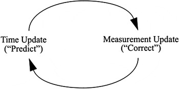
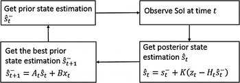
The Kalman filter estimates a process by using a form of feedback control. It estimates the future state of a process and then receives feedback about the actual state in the form of measurements; both the next state estimate and measurement are assumed to contain error (i.e., uncertainty). As such, the Kalman filter estimation consists of both time update equations and measurement update equations. The time update equations are responsible for projecting forward (in time) the current state and error covariance estimates to obtain an a priori estimate for the next (future) time step. The measurement update equations are responsible for the feedback, that is, for incorporating a new measurement with the a priori estimate to obtain an improved a posterior estimate. The time update equations can also be thought of as predictor equations, while the measurement update equations can be thought of as corrector equations, comprising a predictor–corrector algorithm as shown in Figure 4.
The ongoing discrete Kalman filter cycle (Welch & Bishop, Reference Welch and Bishop2006).

5.1.1. Predict equation
The Kalman filter addresses the general problem of trying to estimate the state s ∈ R n of a discrete time controlled process that is governed by a stochastic difference equation (Welch & Bishop, Reference Welch and Bishop2006). The general predict equation, adapted for design as opposed to control, is
 $$s_{t + 1} = f\lpar {s_t\comma \; x_t\comma \; w_t} \rpar = {A_t} {s_t} + Bx_t + w_t \comma $$
where s t is the SoI, x t is the design vector, and w t is a random variable representing the process model error at time t (note that nomenclature is changed from conventional control theory nomenclature for consistency with the design process). The matrix A relates the state s at time t to the state at time t + 1, in the absence of either a driving function or process noise; thus, A is the state evolution model. The matrix B relates the design vector to the SoI s; thus, the B matrix represents the influence of the design on the SoI; thus, B is the design model. In the context of design, s t is a vector of variables that represents the current state (i.e., the current SoI) in which the design is operating, such as the current demand for data service on a satellite system.
5.1.2. Measurement equation
When it is not possible to measure the real value of the uncertain SoI variables, s, directly from the process, we can define the relationship between indirect measurements, z, and the real value of the uncertain SoI variables at time t. The measurement equation z ∈ R m is defined as
 $$z_t = f\lpar {s_t\comma \; v_t} \rpar = H_t s_t + v_t. $$
The m × n matrix H relates the SoI s to the indirect measurements z; thus, H represents the measurement model. The random variable v t represents the model error at time t.
5.1.3. Kalman filter computation
We define
 ${\hat s}_t^{-} \in R^n $
to be a prior state estimate at step t given knowledge of the process prior to step t, and
 ${\hat s}_t \in R^n $
to be a posterior state estimate at step t given measurement z
t
. We can define prior and posterior estimate errors as
 $${\hat e}_t^ - = {\hat s}_t - {\hat s}_t^ {-} \comma \, $$
 $${\hat e}_t = s_t - {\hat s}_t. $$
Then, the prior estimate error covariance is defined as
 $$P_t^ - = E\lsqb {{\hat e}_t^ - {\hat e}_t^ {-T}} \rsqb\comma $$
while the posterior estimate error covariance is given by
 $$P_t = E\lsqb {{\hat e}_t {\hat e}_t^T} \rsqb. $$
The equation for the posterior state estimate
 ${\hat s}_t $
is derived as a linear combination of the prior estimate
 ${\hat s}_t^{-}$
and a weighted difference between an actual measurement z
t
and a measurement prediction
 $H_t {\hat s}_t^{-}$
in Eq. (7):
 $${\hat s}_t = s_t^{-} + K\lpar {z_t - {H_t} {\hat s}_t^{-}} \rpar. $$
The difference
 $\lpar {z_t - H_t {\hat s}_t^{-}} \rpar $
in Eq. (7) is called the measurement residual. The residual reflects the discrepancy between the predicted measurement
 $H_t {\hat s}_t^{-} $
and the actual measurement z
t
. A residual of zero means that the two are in complete agreement. The n × m matrix K is the Kalman gain, which minimizes the prior estimate error covariance. Formulations for the Kalman gain can be found in the controls literature; one well-known form of the Kalman gain is given as Welch and Bishop (Reference Welch and Bishop2006):
 $$K_t = \displaystyle{{P_{t}^{-} H_t^{T}} \over {H_t P_{t}^{-} H_t^{T} + R_t}}\comma $$
where R
t
is the measurement model error covariance [(
 $v \sim N\lpar {0 \comma \,R} \rpar $
].
5.1.4. Optimal estimation
We apply the Kalman filter time update equations to obtain the optimal estimation of the future state s t+1. The linear Kalman filter time update equations are given by Eqs. (9) and (10),
 $${\hat s}_{t + 1}^ - = A_t {\hat s}_t + Bx_t\comma $$
 $$P_{t + 1}^ - = A_t P_t A_t^T + Q_t\comma $$
where the – sign indicates a prior estimate, and Q
t
is the error covariance of the predict model
 $\; [w \sim N\lpar {0 \comma \,Q} \rpar $
]. Estimation of the update Eqs. (3)–(10) follows the standard approach outlined in Welch and Bishop (Reference Welch and Bishop2006). Figure 5 clarifies steps to obtain the optimal estimation of future states using the Kalman filter.
Steps to obtain optimal state estimation through Kalman filter.

5.2. Design selection
The Kalman filter approach treats the design process as a stochastic control problem, in which the design is used to manage the uncertainty throughout the life cycle of the system. The SoI is used to describe particular states of an uncertain parameter that may change over time. Given the Kalman filter estimation of the SoI, an optimization model is developed to select the best design for future time steps. The SoI may appear in the optimization model within the objective function or a constraint function (or both). In the proposed approach, the SoI is assumed to be observed in discrete time. Based on the optimal estimation outlined in Figure 5, we select the design variable values, using optimization, based on the forecasted SoI in future time periods t, with the complete design process shown in Figure 6. A key challenge in this optimization problem is that for the general Class 3 design case, the SoI forecast, s t+1, is a function of the optimized design x t for time period t; however, the SoI forecast is required to quantify the objective function of the design optimization problem needed for design selection. Thus, the state estimation of Eq. (9) is coupled with the design selection problem; an efficient means of solving this coupled set of equations must be identified. In the following section, we apply our approach to optimize the design of a communication satellite constellation under uncertain demand for data. We employ a decoupled approach to solving the problem to alleviate the coupling issue previously discussed.
Flowchart of the proposed approach.

6. CASE STUDY: COMMUNICATION SATELLITE CONSTELLATION
In this section, we apply our methodology for designing a LEO communication satellite constellation. The methodology allows prediction of the total system capacity versus total life cycle cost for a given communication quality. The design vector includes orbital altitude, h, the satellite transmitter power, P T, the antenna size, A D, and the number of satellites, N t . As has been described previously, both IRIDIUM and GLOBALSTAR met or exceeded given technical requirements, yet they both were economic failures. It appears that the reasons for system success or failure is not strictly determined by adherence to design phase requirements, but rather in the system design over the entire life cycle. The system design must respond to the combination of aleatory and epistemic uncertainties that ultimately determine the success of the system.
A communication satellite constellation is a group of satellites that respond to a specific global data demand, such as phones or pagers (Wertz, Reference Wertz2012). The greatest epistemic uncertainty that a communication satellite constellation faces is the number of users and hence demand for data (de Weck et al., Reference de Weck, Eckhart and John2007). In a new approach, de Weck et al. (Reference de Weck, Scialom and Siddiqi2008) suggests designing reconfigurable satellite systems by adding the ability to change the satellites’ orbits. Based on the orbital change concept, a case study is developed to show the application of a Kalman filter to quantify demand (number of users) when a sudden unexpected change occurs.
6.1. Demand prediction with Kalman filter
It is assumed that the initial required capacity for a new communication satellite constellation is initially 50,000 channels, and it increases at an uncertain rate during the 15 years of the system lifetime, T sys. The needed channel capacity, N ch, is calculated based on market studies and best guess extrapolations of current demand. The two quantities that have to be estimated are the expected global number of subscribers, N user, as well as their average individual activity level, A user (min/month). The number of (duplex) channels that the system has to provide to satisfy this demand, N ch, represents the instantaneous capacity requirement (de Weck et al., Reference de Weck, Neufville and Chaize2004):
 $$N_{{\rm ch}} = \displaystyle{N_{\rm user} \cdot A_{\rm user} \over U_{\rm s} \cdot \displaystyle{365 \over 12} \cdot 24 \cdot 60}\comma $$
where U s is the global system utilization, a fraction between 0 and 1. For a new satellite constellation, we assume a global subscriber base of N user = 2 × 10⁶ and an average monthly user activity of A user = 110 min/month. Global system utilization, U s, is typically around 0.1 according to Lutz et al. (Reference Lutz, Werner and Jahn2012). This number captures the fact that only a fraction of satellites is overinhabited, revenue-generating terrain at any given time. Substituting these values in Eq. (13) results in a constellation capacity of N ch = 50,228.
It is assumed that we initially launch the constellation consisting of four satellites to the circular orbit of altitude 800 km, antenna size of 1.5 m, and transmitter power of 200 W to meet the near-term demand for data. To formulate an objective function for the design, we use total life cycle cost (LCC). According to de Weck et al. (Reference de Weck, Neufville and Chaize2004), LCC includes satellite manufacture, validation testing, launch, deployment, ground station operations, and replenishment. For the proposed initial design, the LCC is approximately $124 million. Because demand is uncertain, there might be significant excess capacity in the system, as in the IRIDIUM and GLOBALSTAR cases. In these cases, the revenue stream may be insufficient to recuperate the initial investment. If the actual market is only 10,000 users instead of 100,000, the capacity must be viewed as a wasted investment. Therefore, it is critical that the system be flexible to allow system reconfiguration to ensure positive revenue.
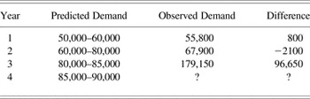
While we have selected an initial design (i.e., t = 0), one would want the ability to adjust the capacity of the system to the evolving demand in future time periods. We make estimations of future demand containing interval uncertainty; future demand intervals are estimated using a known methodology, such as evidence theory (Agarwal et al., Reference Agarwal, Renaud, Preston and Padmanabhan2004), and are shown in Table 1. For the case study in this section, we assume that the satellite system has been built with flexibility and therefore will be updated as the demand changes. To demonstrate the methodology, it is assumed that we have estimated predicted demand ranges for the life cycle of constellation, but have only observed demand through Year 3. In this example, the actual observed demand remains within the predicted intervals of Table 1 in the first 2 years, while a sharp unexpected increase in demand occurs in Year 3.
Data simulation for constellation demand

The Kalman filter is now applied to quantify the future state of demand in Year 4 (i.e., t = 4). In this case study, we attempt to estimate the SoI that is the demand, quantified as number of channels N
ch, for the next year. For the measurement model, we estimate the demand as a function of users using Eq. (11); however, because Eq. (11) is an estimate, we assume an error of 10% measurement noise,
 $R = 10\% $
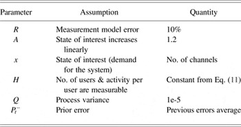
(i.e., number of users cannot be measured exactly). We assume that our process is governed by the linear difference equation [Eq. (1)] and that the SoI linearly increases from year to year based upon our demand model, leading to a state evolution term A = 1.2. The noisy measurement z is the number of users that is related to SoI through Eq. (11), and H is assumed to be constant in the measurement equation. Presuming a small process variance, we let Q = 1e-5. An initial value for
 $P_t^ - $
can be computed as the average of previous errors. Table 2 presents the assumptions that are applied in this simplified case study.
Kalman filter assumptions for the case study

Applying Eqs. (3)–(10), we estimate the demand (SoI) for the next time step, t + 1 = 4, as 188,815 channels, shown in Table 3. As the following section describes, the optimal estimation of needed channels for Year t = 4 enables the ability to choose the best design to meet the new market demand.
Results of Kalman filter for the case study

6.2. Design optimization
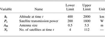
As shown in the previous section, the output of the Kalman filter is the optimal estimation of demand for the next time steps. While the Kalman filter provides an estimate of the future states, it does not provide the optimal design for the future state. The design vector for the LEO communication constellation includes the orbital altitude, h, the satellite transmitter power, P T, the antenna size, A D, and the number of satellites, N t . It is assumed that some parameters like the allocated frequencies and bandwidth are fixed; this is a realistic assumption as frequencies and bandwidth are not under the control of the system designers. Equation (12) represents the design vector.
 $$x_t = \lsqb {h_t\comma \; N_t\comma \; A_{\rm D}\comma \,P_{\rm T}} \rsqb. $$
Each feasible vector x defines a particular design for the communication satellite constellation. Table 4 shows the bounds for design variables in design vector x.
LEO constellation design vector
 ${\bf x}$

An important constraint to consider in the system design is the total designed capacity of the communication satellite system, CapTot, to ensure that demand is met. The capacity CapTot is a function of the power received, P R, as well at the number of satellites, N t , and hence is a function of the four design variables [Eq. (12)]. Equation (13) shows that capacity must be greater than or equal to demand (min) at a time t:
 $$\hbox{Cap}_{{\rm Tot}} \lpar {P_{\rm R}\comma\,N_t} \rpar \ge \mathop \sum \limits_{y = 1}^{T_{{\rm sys}}} [A_{{\rm ch}} N_{{\rm ch}} ]\comma$$
where demand is quantified with A ch, the annual average use of the system per channel [min] and N ch, the number of channels to meet demand (i.e., the SoI). The received power P R is a function of the antenna size, altitude, and the transmitted power. The Friis transmission equation [Eq. (14)] presents the relationship (Richharia, Reference Richharia1995):
 $$P_{\rm R} = P_{\rm T} \times G_{\rm T} \times G_{\rm R} \times \left( {\displaystyle{{\rm \lambda} \over {4{\rm \pi}}}} \right)^{2} \times \left( {\displaystyle{1 \over h}} \right)^{2} \times A_{\rm D}^2\comma $$
where P R is the power received (W), P T is the power transmitted (W), G T is the gain of the transmit antenna (constant), G R is the gain of the receive antenna (constant), λ is the wavelength, and A D is the antenna size (m). This equation essentially states that the strength of the received signal is a function of the strength of the original transmitted signal, the antenna size, the wavelength corresponding to the frequency of operation, and the altitude of satellite.
Equation (15) is the model for the system objective function. The objective function J captures all the metrics by which the goodness of a particular design can be evaluated. The objective function contains the life cycle cost, the cost of changing the satellite system design, and the profit obtained from the service that the system can provide.
 $$J = \hbox{min}\left\{ {\mathop \sum \limits_{y = 1}^{T_{{\rm sys}}} \hbox{LCC} + \mathop \sum \limits_{y = 1}^{T_{{\rm sys}}} \hbox{DCC} - \mathop \sum \limits_{y = 1}^{T_{{\rm sys}}} (\hbox{CPF} \times N_{{\rm ch}} )} \right\}.$$
The life cycle cost is the sum of the research and development, test and assembly cost, the manufacturing cost, the launch cost, the space and ground operation cost, and the replacement costs. The T sys is the total of years that we expect the system provides the service; in this study, we assume T sys is 15 years. The CPF is the cost for service to users and the number of channels is the estimated SoI; the product of CPF and N ch represents profit. The summation of the costs in the objective function should be recovered by the profit obtained from the users.
A primary main element of the objective function is the cost of changing the system design, given by Eq. (17). The DCC (from time i to time j) includes costs of adding new satellites, the cost of reorbiting existing satellites, and changing the antenna size and power transmitter:
 $$\hbox{DCC} = \mathop \sum \limits_1^y \lpar {N_i C_{ij}} \rpar + \lpar {N_j - N_i} \rpar C_{{\rm new}} + C_{\rm A}\comma $$
where i is the time step in which design decision is made, j is the future time step in which a design decision is implemented, N i , N j is the number of satellites at times i and j, C ij is the cost of changing the orbit between altitudes h i and h j , C new is the total cost of adding a new satellite to the constellation, and C A is the cost of changing the antenna size.
The C new includes satellite manufacturing, validation testing, launch, deployment, ground station operations, and replenishment. The new satellite costs are determined from a cost model, SVLCM (Siddiqi, Reference Siddiqi2006), which provides a rough order of magnitude cost estimate based on the dry mass of the spacecraft. The model gives estimates of the development and production costs of unmanned Earth-orbiting spacecraft. The SVLCM is a top-level model derived from the NASA/Air Force Cost Model database (Siddiqi, Reference Siddiqi2006). The reorbiting cost, C ij , contains the cost of delay, fuel, and propulsion (Minoli, Reference Minoli2015):
 $$C_{ij} = \vert {\lpar {N_j - N_i} \rpar \; \Delta v_{ij}} \vert (C_{{\rm F\;}} + C_{\rm P} + C_{{\rm D}} )\comma$$
where Δv ij is the velocity change between altitudes h i and h j , C F is the cost of fuel to move the satellite from h i to h j , C P is the cost of propulsion to move the satellite from h i to h j , and C D is the cost of delay in data transferring during the orbit reconfiguration.
The cost of orbital change is a function of excessive fuel that satellites carry. According to data from NASA, $15,800 is the average cost of launching 1 kg of mass to LEO (Siddiqi, Reference Siddiqi2006). The cost of fuel to move from h i to h j is a function of the required Δv ij and the mass of the satellite, M:
 $$C_{\rm F} = f\lpar {\Delta v\comma\; M} \rpar. $$
Equation (19) presents the Hohmann rule to calculate Δv ij (Belbruno & Miller, Reference Belbruno and Miller1993; Rauwolf & Coverstone-Carroll, Reference Rauwolf and Coverstone-Carroll1996):
 $$\Delta v_{ij} = \sqrt {\displaystyle{{\rm \mu} \over {h_i}} \;} \left(\displaystyle{ \sqrt {{{2 \,\ast\, {h_j}} \over {h_i + h_j}}} - 1}\right).$$
In this equation, μ is the standard gravitational parameter of the satellite, obtained by multiplying standard gravity (9.806 m/s2) by the mass of the satellite (and h is altitude).
6.3. Results and discussion
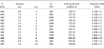
To find the optimal design for the constellation that meets the Kalman filter demand estimate of 188,815 channels (or 2.37e + 12 min), it is necessary to formulate an optimization problem: this is accomplished based upon minimizing the objective function of Eq. (15) subject to the capacity constraint of Eq. (13). Based upon the optimization model developed by de Weck and Chang (Reference de Weck and Chang2002), a Pareto optimal set of nondominated solutions that meet the capacity constraint can be extracted, shown in Table 5. An optimal system design for the next time period, that is, period t + 1 = 4, is obtained as x 4[h 4 = 400 km, N 4 = 8, P T = 1800 W, A D = 3.5 m]. The new design vector represents changing the current four satellites’ orbits from 800 to 400 km and deploying four additional satellites to meet the new demand. In addition, it requires the antenna length be increased from 1.5 to 3.5 m, and the power be increased substantially through the addition of significantly more solar panels to the constellation. The initial constellation was designed to fulfill the initial demand of 50,000 channels and up to the 100,000 channels. However, market changes led to an unexpected increase in demand for this constellation service at t = 3 (i.e., Year 3) and hence higher demand in Year 4 as estimated by the Kalman filter. The total cost of redesigning the constellation from initial design to the new configuration is estimated to be $265.32 million. If the initial constellation were designed without flexibility, retiring that constellation and launching eight new satellites to meet the new market would cost a minimum of $391 million.
Set of Pareto optimal constellation designs to meet the estimated demand of 2.37E+12 (min) obtained from Kalman filter

7. CONCLUSION
This paper presents a resilient design methodology for complex systems. We reviewed the concept of resilient design and its value in engineered systems. Because engineered systems face a variety of epistemic uncertainties, they should be designed with resiliency to be able to overcome the epistemic uncertainties. With the example of IRIDIUM, we showed that the resiliency of an engineered system subject to epistemic uncertainty can be the difference between financial success and failure of the system. We proposed a resilient dynamic design approach for engineering systems. In this approach, we apply the Kalman filter to handle epistemic uncertainty and obtain the optimal estimation of future states of interest. Based upon this estimation, and through developing an optimization problem, we are able to maintain an optimal design throughout the system life cycle.
We presented a case study of a communication satellite constellation, showing how the Kalman filter approach treats design as a stochastic control problem, demonstrating that four flexible design variables can be changed to keep the system operating optimally according to a user-selected objective and constraints. This provides the system designers with a self-updating design, negating the need to reengineer the system whenever operation conditions fall outside of their expected ranges.
Future work to extend this method to actual system design includes testing the methodology on a wider range of design problems with varying levels of complexity, as well as addressing the difficulties in estimating the coupled state estimation (i.e., Kalman filter) equations and design optimization problem.
ACKNOWLEDGMENTS
This research was funded in part by the National Science Foundation (Project CMMI 1349787). The opinions, findings, conclusions, and recommendations expressed are those of the authors and do not necessarily reflect the views of the sponsor.
Elham Keshavarzi is a PhD candidate at Oregon State University. She received an MS in industrial engineering from K. N. Toosi University in 2010. She is currently seeking a PhD in mechanical engineering under Dr. Chris Hoyle. Before returning to academia, she worked for the Saman Electronic Payment Company for 2 years as a Data Scientist and Project Manager. Her research is focused on uncertainty management, decision making in engineering design, statistical data analysis, resilience and safety analysis, and optimization of complex systems.
Matthew McIntire is a graduate student at Oregon State University. He received a BS in engineering and applied science from Seattle Pacific University in 2008 and is currently a PhD candidate in mechanical engineering under Dr. Chris Hoyle. Before returning to academia, he worked for 3 years in Guatemala as a missionary-engineer. His research is focused on uncertainty, statistical data analysis, modeling, safety analysis, and optimization of complex systems.
Christopher J. Hoyle is an Assistant Professor in design in the Mechanical Engineering Department at Oregon State University. He received his PhD in mechanical engineering from Northwestern University in 2009 and his Master's in mechanical engineering from Purdue University in 1994. His areas of expertise are uncertainty propagation methodologies, Bayesian statistics and modeling, stochastic consumer choice modeling, optimization, and design automation. Dr. Hoyle is coauthor of the book Decision-Based Design: Integrating Consumer Preferences Into Engineering Design. His current research interests are focused upon decision making in engineering design, with emphasis on the early design phase.