Introduction
The recent upswing in antenna research has heightened the need for efficient alternate methods of developing phased array antennas for advanced, cutting-edge applications, such as beamforming and beam steering. Due to the incorporation of “Time” as a fourth control parameter alongside the existing controls of amplitude, phase, and element spacing, time-modulated arrays have been proposed as potential substitutes for traditional antenna arrays [Reference Maneiro-Catoira, Brégains, García-Naya and Castedo1]. The idea behind time-modulation is to regulate the ON and OFF switch timings of the array elements to produce the required phase divergence for phase tapering [Reference Rocca, Yang, Poli and Yang2]. Shifted switching instants in a time-modulated antenna array can effectively support advanced adaptive beamforming applications with scanned patterns in predetermined directions [Reference Tong and Tennant3]. Compared to traditional mechanical steering techniques, this electronic control can more effectively synthesize the radiating properties of the antenna [Reference Li, Chen and Yang4]. In addition, these alternative arrays have the intrinsic advantage of having lower sidelobes with appropriate switching [Reference Yang, Gan, Qing and Tan5]. Due to the incorporation of the timing function, multiple sidebands or harmonic frequencies are produced by the Fourier transformation of coefficients from the time domain to the frequency domain [Reference Poli, Rocca, Oliveri and Massa6]. Though the harmonics cause power loss in unwanted directions, they can also be exploited to generate multiple patterns simultaneously [Reference Bregains, Fondevila-Gomez, Franceschetti and Ares7]. The possible exploitation of harmonics has been reported for electronic scanning, and new methods to create simultaneous beams have emerged [Reference Shanks8, Reference Li, Yang, Chen and Nie9]. Initial research on time-modulation has shown substantial improvements in pattern synthesis by reducing sidelobes [Reference Yang, Gan and Tan10–Reference Poddar, Paul, Chakraborty, Ram and Mandal12]. For efficiency enhancement, reducing sidelobes has become essential [Reference Maneiro-Catoira, Bregains, Garcia-Naya and Castedo13–Reference Chen, Liang, He, Fan, Zhu, Jin and Geng15]. Controlling sidebands or harmonics and suppressing power in random directions also became a major research focus in time-modulation with the advent of optimization algorithms [Reference Yang, Gan and Qing16–Reference Poli, Rocca and Massa20]. In this context, shifting and splitting of time durations helped to lower the side beam power [Reference Poli, Rocca, Manica and Massa21, Reference Poli, Moriyama and Rocca22]. The combination of shifted pulse and optimization algorithm has also been reported to simultaneously reduce sidelobes and sidebands [Reference Poli, Moriyama and Rocca22–Reference Tan, Hu, Dong, Li and Zhou24]. In this respect, optimization methods helped achieve optimal time schemes to lower the higher-sideband power and the sidelobes of the main beam [Reference Chakraborty, Ram and Mandal25–Reference Chakraborty, Ram and Mandal27]. Optimization algorithms have also been employed to optimize the ON-time instants and the durations of the shifted and splitting pulses of time-modulated antennas for harmonic beam suppression [Reference Yang, Gan and Peng Khiang28–Reference Zhu, Yang, Zheng and Nie30]. In the later stages, other means of utilizing sideband radiation to create the desired multi-harmonic beam patterns have also emerged [Reference Chakraborty, Singh, Gupta, Ram and Mandal31]. The advantages of simultaneously produced beams for multi-point transmission have also gained momentum [Reference Chakraborty, Ram and Mandal32–Reference Ram35]. Significant improvements in harmonic steering have been demonstrated through mathematical exploitation of the array phase center [Reference Chakraborty, Ram and Mandal36–Reference Yang, Gan and Tan38]. Time-modulated arrays are suitable for radar applications because of their electronic steering capability [Reference He, Yi, Chen, Zhu, Liang, Geng and Jin39]. Monopulse radar application with concurrent sum-difference beams also became easier because a single optimized beamforming network can generate both beams using the inherent sidebands in time-modulation [Reference Gang, Yang and Nie40–Reference Rocca, Poli, Oliveri and Massa42]. In addition, the concept has been used to develop several scanned beam patterns for multifunction radars with good scanning coverage [Reference Chakraborty, Ram and Mandal43]. Researchers have also focused on null placement across a wide angular region to further explore harmonic controlling for radars [Reference Poli, Rocca, Oliveri and Massa44, Reference Chakraborty, Mishra, Singh, Ahmad, Khan, Sharma, Alkhayyat and Gupta45]. Time-modulation has also been used for more advanced applications, such as shaped beam pattern generation [Reference Chakraborty, Saxena, Verma, Juyal, Gupta, Singh, Ram and Mandal46–Reference Li, Yang, Huang and Nie48], and for cognitive radios by exploiting its harmonics [Reference Rocca, Zhu, Bekele, Yang and Massa49, Reference Bhattacharya, Saha and Bhattacharyya50]. Due to the adaptability and capabilities of optimized timing frameworks, time-modulated arrays have emerged as an efficient alternative to conventional phased arrays.
The research in this article further extended the time-modulation concept by proposing several optimal timing frameworks to generate an efficient sidelobe canceller beamformer for radars. The first objective is to design an adaptive sidelobe canceller beamformer that enables simultaneous multi-pattern scanning across different angular regions and suppresses the sidelobes of the scanned beams to a satisfactory level for interference rejection. The pulse-shifting and splitting methods, with optimized switch instants, are combined to generate optimal scanned beams for radar. The second objective is to place a deep null in a particular angular region to cancel out the transmission in that region by producing a zero-signal space for jamming. The third objective is the extended version of the second, in which sectorized anti-jamming is targeted using a single beamformer by controlling the harmonics. The objectives have been framed with real-time radar application in mind, where electronic beam scanning, sidelobe reduction, null control, and jamming mitigation are required. The specific objectives of this research, and the methods proposed for that, are elaborated as follows.
First, a time-modulated sidelobe canceller beamforming antenna is designed to suppress the interfering signals impinging on the sidelobes of the simultaneously scanned beams. The objective is to generate multiple scanned beams at prespecified directions ranging from 45° to 135°, covering a broad scanning area of around 90° in the broadside. For this purpose, the timing frameworks of an 8-element antenna are optimized so that the different optimized start instants of each antenna create a cumulative phase divergence in the overall radiation pattern. The mathematical foundation behind this approach is derived. The proposed beamformer can reduce sidelobes, and in the proposed research, the sidelobe levels (SLLs) of all scanned patterns are suppressed below 20 dB. Mathematically, the main beam consumes the maximum power in time-modulation. The first-harmonic beams on the positive and negative sides consume the second-largest power among the other higher harmonics. The scanning coverage is controlled by directing the first negative side beam toward 75°, 60°, and 45°, and the first positive side beam toward 105°, 120°, 135°, with scanning coverages of 30°, 60°, and 90°, respectively. The proposed beamformer also ensures that the SLLs of the scanned positive and negative beams, along with the main beam pattern, are below the standard levels for interference mitigation and unnecessary power radiation in random directions. The beamforming timing frameworks are employed with 8-element linear and symmetric time-modulated antenna arrays to validate the proposed approach.
Second, the adaptabilities of the beamformer are further tested for the strategic null placements in the direction of jammers. The strategic nulls can be placed by generating a zero-signal space in the broadside angular region so that the interfering signals can be efficiently blocked by concentrating only on the desired one. The proposed beamformer is aimed at placing nulls in a single direction as a single-point jammer, as well as for a sectorized jammer. The first-harmonic beam patterns are used to address the single nulls in the radiation pattern of an 8-element time-modulated antenna, while keeping the central beam constant. Two different cases are targeted by aiming the first-positive and first-negative harmonics toward null points at 40°, 60°, and 140°, 120°, respectively. To further extend the concept and to assess whether the proposed beamformer is adaptable enough to suppress signals across a broad region, sectorized jamming is targeted. Different cases of sectorized jamming are aimed at suppressing signals in the regions 0° to 65° and 40° to 80° using positive harmonics. Due to the symmetric nature of the linear array and the symmetry of the harmonics, the sectorized jamming is targeted from 115° to 180° and from 100° to 140°, with negative harmonics. The beamformer ensures the SLLs of all the patterns are below the standard requirements. The sectorized jamming targets signals below 30 dB across a broad region. For all scanning and jamming objectives, the central pattern is kept fixed in the broadside direction to optimize power usage. The efficient design of the beamformer also concentrates the maximum amount of power on the main beam and the first harmonic beams, thereby enhancing overall efficiency. For all the objectives, optimal switching instants and the ON time durations of the array ensure the efficiency of the proposed method. So, an efficient optimization method is needed to design an efficient time-modulated beamformer. The Particle Swarm Optimizer (PSO) has long been used to solve real-time engineering problems. PSO has also been rigorously applied to array radiation pattern synthesis. But it lacks efficiency and drastically increases the computation speed when too many objectives are targeted simultaneously. To overcome the limitations of PSO, a powerful quantum-inspired PSO is employed in this research to simultaneously optimize multiple objectives targeted by the proposed beamformer. The quantum-inspired PSO algorithm provides the much-needed efficient solutions for the beamformer and makes it a standout performer for efficient time-modulated radar systems.
The remaining part of the research is organized as follows: Section 2 describes the mathematical foundation of the time-modulated beamformer, where a detailed insight into a generalized time-modulated array and the incorporation of time schemes into its radiation pattern are provided. The construction of the symmetric array beamformer with pulse shifting and splitting, considering the effect of harmonics on radiation power efficiency, is also formulated. The quantum-inspired PSO metaheuristic is presented in Section 3. The performance of the proposed beamformer as sidelobe canceller, single-point anti-jammer, and sectorized anti-jammers is analyzed in Section 4. The conclusive remarks and the future scopes are presented in Section 5.
Time-modulated beamformer design
Time-modulation includes a new control parameter, “Time”, into the synthesis of array radiation patterns by mathematically modifying the array factor. The time-to-frequency domain conversion of the switching function provides an edge over traditional radiation pattern synthesis. The general mathematical modeling of the array response for an N-element symmetric linear antenna array connected with radio frequency (RF) switches, shown in Fig. 1, can be given as [02]
 \begin{equation}A{F_S}\left( {\theta ,t} \right) = {e^{\left(\,{j2\pi {f_0}} \right)t}}.2\mathop \sum \limits_{n = 1}^{N/2} \left[ {{I_n}{U_n}\left( t \right){e^{\left\{ {j\beta \left( {\frac{{2n - 1}}{2}} \right)dcos\theta } \right\}}}} \right]\end{equation}
Generalized time-modulated beamforming structure with “N” antennas and switches.

Figure 1 Long description
The diagram illustrates a beamforming structure featuring multiple single-pole single-throw (SPST) switches labeled from 1 to N. Each switch is connected to a power divider/combiner. The switches are arranged in a linear sequence, with connections leading to a control board. The power divider/combiner is linked to a summing point, which then connects to the output. The diagram includes a notation for an angle theta, indicating a phase or directional component. The control board manages the operation of the switches, influencing the output signal. The structure is designed for signal processing and directionality control.
The above expression shows the symmetric arrangement of “N” elements where the switching sequences of the elements in the left half are the same as the right half of the array elements. The beamformer in Fig. 1 shows “N” radiators connected to a power combiner via RF single-pole-single-throw (SPST) switches. The control board can provide the necessary tapering by controlling the ON and OFF timings of each radiator, and the responses from each radiator are summed to produce the synthesized radiation pattern. In equation (1),  ${U_n}\left( t \right)$ represents the time-modulated switching sequences for each element from n = 1 to N,
 ${I_n}$ is the current amplitude,
 ${f_0}$ denotes the central beam frequency,
 $\beta $ is the wave propagation constant,
 $d$ is the spacing between each radiator, signals are impinging at an angle
 $\theta $ to the array main axis,
 $t$ represents the time instants within the modulation period, and
 $A{F_{{\text{Symmetric}}}}\left( {\theta ,t} \right)$ stands for the overall array response after incorporating the time-modulation in a linear symmetric antenna array. Due to the periodicity of the timing function,
 ${U_n}\left( t \right)$ can be presented as [02]
 \begin{equation}{U_n}\left( t \right) = \mathop \sum \limits_{m = - \infty }^\infty \left[ {{a_{mn}}{e^{jm\left( {2\pi {f_p}} \right)t}}} \right]\end{equation}
Here,  ${a_{mn}}$ is the coefficient of excitation translated from the frequency to the time domain and represents the “m” number of frequency components for the n-th radiator. The frequency components, inherently generated by time-modulation, are called harmonics; where
 $m = 0$ represents the main beam, and
 $m = \pm 1,\, \pm 2,\, \pm 3,\, \ldots ,\, \pm \infty $ correspond to the sidebands at multiple positive and negative harmonics. The excitation coefficient
 ${a_{mn}}$ at time-modulation frequency (
 ${f_p}$) with a modulation period
 ${T_p}$ (
 $1/{f_p}$) can be extended as [02]
 \begin{equation}{a_{mn}} = \frac{1}{{{T_p}}}\mathop \int \limits_0^{{T_p}} {U_n}\left( t \right){e^{ - jm\left( {2\pi {f_p}} \right)t}}\,dt\,\,\,\,\,\,\,\,\,\end{equation}
Putting the excitation coefficient into the antenna array response, the time-modulated response is modified as
 \begin{equation}A{F_S}\left( {\theta ,t} \right) = {e^{\left( {j2\pi {f_0}} \right)t}}.2\mathop \sum \limits_{n = 1}^{N/2} {I_n}\left[ {\mathop \sum \limits_{m = - \infty }^\infty {a_{mn}}{e^{jm\left( {2\pi {f_p}} \right)t}}.{e^{\left\{ {j\beta \left( {\frac{{2n - 1}}{2}} \right)dcos\theta } \right\}}}} \right]\end{equation}
Further, the simplified array response for the “m” number of frequency components can be presented as
 \begin{equation}A{F_m}\left( {\theta ,t} \right) = {e^{j2\pi \left( {{f_0} \pm m{f_p}} \right)t}}.2\mathop \sum \limits_{n = 1}^{N/2} \left[ {{I_n}{a_{mn}}{e^{\left\{ {j\beta \left( {\frac{{2n - 1}}{2}} \right)dcos\theta } \right\}}}} \right]\end{equation}
The time-modulated array generates the central pattern at  $m=0$, and the harmonics are generated at
 $m = \pm 1,\, \pm 2,$
 $\pm 3,\, \ldots ,\, \pm \infty $. The main beam, the first positive and the first negative harmonics responses of the N-element array can be given as
 \begin{equation}A{F_0}\left( {\theta ,t} \right) = {e^{j2\pi \left( {{f_0}} \right)t}}.2\mathop \sum \limits_{n = 1}^{N/2} \left[ {{I_n}{a_{mn}}{e^{\left\{ {j\beta \left( {\frac{{2n - 1}}{2}} \right)dcos\theta } \right\}}}} \right]\end{equation}
 \begin{equation}A{F_{ - 1}}\left( {\theta ,t} \right) = {e^{j2\pi \left( {{f_0} - {f_p}} \right)t}}.2\mathop \sum \limits_{n = 1}^{N/2} \left[ {{I_n}{a_{mn}}{e^{\left\{ {j\beta \left( {\frac{{2n - 1}}{2}} \right)dcos\theta } \right\}}}} \right]\end{equation}
 \begin{equation}A{F_{ + 1}}\left( {\theta ,t} \right) = {e^{j2\pi \left( {{f_0} + {f_p}} \right)t}}.2 \sum\limits^{N/2}_{n = 1} \left[ {{I_n}{a_{mn}}{e^{\left\{ {j\beta \left( {\frac{{2n - 1}}{2}} \right)dc{\text{os}\theta }} \right\}}}} \right]\end{equation}
In this research, the first negative harmonics at  $m = - {\text{1}}$ and the first positive harmonics at
 $m = {\text{ + 1}}$ are exploited for beam scanning and jamming in radars. Thus, it is very important to suppress higher harmonics and SLLs to conserve power and ensure efficient transmission and reception of the array. Furthermore, phase-divergence characteristics are also proposed for optimized shifted pulses in the beamformer, which need to be investigated for radiation pattern synthesis. Detailed mathematical modeling of power transmission and time-scheme modulation is also required to develop a multipurpose beamformer for scanning, jamming, and other advanced applications in modern radar systems.
Mathematical modeling of time schemes
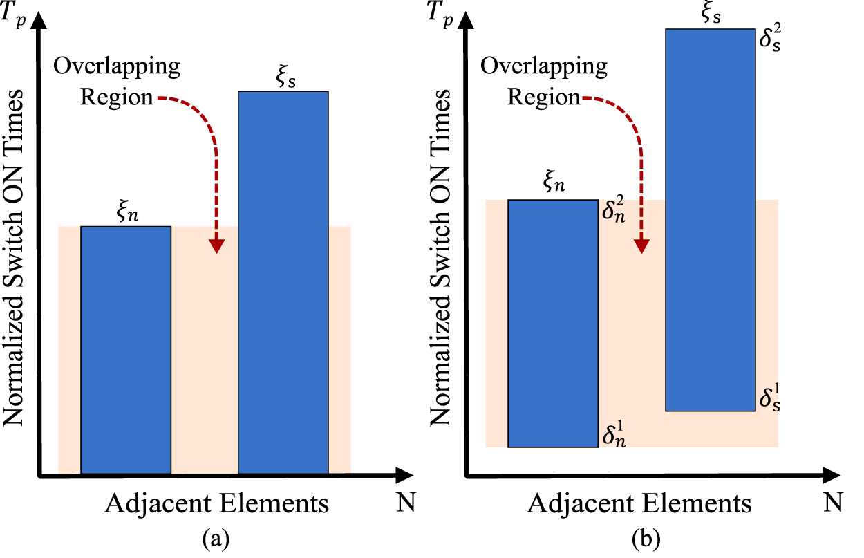
The inherently generated side beams at multiple harmonics are generally considered a source of power loss but can be exploited for specific purposes. So, proper mathematical modeling is required to assess the sideband levels (SBLs) of the desired as well as higher-order harmonics. The closed-form derivatives of a simple pulse and a shifted pulse are derived in this subsection. The possible switching schemes are shown in Fig. 2(a) and (b), where Fig. 2(a) shows a simple time scheme for two adjacent radiators, and Fig. 2(b) shows the same pulse scheme for shifted adjacent pulses. The first pulse scheme shows the n-th and s-th adjacent radiators with normalized time periods  ${\xi _n}$ and
 ${\xi _s}$ within the modulating period (
 ${T_p}$), given by
 ${\xi _n} = \left( {{\tau _n}/{T_p}} \right)$ and
 ${\xi _s} = \left( {{\tau _s}/{T_p}} \right)$. The
 ${\tau _n}$ and
 ${\tau _s}$ are the time durations without normalization. The second scheme shows the shifted n-th and s-th pulses with normalized start instants
 $\delta _n^1$ and
 $\delta _s^1$. The pulses end at
 $\delta _n^2$ and
 $\delta _s^2$, respectively, within the modulation period. Figure 2 shows overlapping regions between adjacent time schemes, and the importance of these overlapping pulses is discussed in detail throughout the mathematical modeling of radiated power. Considering all the “m” harmonic responses, the overall array factor can be simplified from equation (4) as
 \begin{equation}A{F_m}\left( {\theta ,t} \right) = \mathop \sum \limits_{m = - \infty }^\infty \left| {{A_m}\left( \theta \right)} \right|{e^{j2\pi \left( {{f_0} \pm m{f_p}} \right)t}}\end{equation}
 \begin{equation}{\text{Here,}}\,{A_m}\left( \theta \right){ } = 2\mathop \sum \limits_{n = 1}^{N/2} {I_n}{a_{mn}}{e^{\left\{ {j\beta \left( {\frac{{2n - 1}}{2}} \right)dcos\theta } \right\}}}\,\,\end{equation}
(a) Simplified time scheme and (b) Shifted pulse time scheme for the n-th and s-th adjacent elements.

The total power transmission can be given as
 \begin{align}{P_T}\left( \theta \right) &= \left\{ {\frac{1}{2}\mathop \sum \limits_{m = - \infty }^\infty {{\left| {{A_m}\left( \theta \right)} \right|}^2}} \right\} \nonumber\\
& = \left\{ {\frac{1}{2}{{\left| {{A_0}\left( \theta \right)} \right|}^2} + \frac{1}{2} \sum^{\infty}_{m=-\infty,\atop{m\neq 0}} {{\left| {{A_m}\left( \theta \right)} \right|}^2}} \right\} \nonumber\\
&= {P_0}\left( \theta \right) + {P_{SB}}\left( \theta \right)\,\end{align}
Here,  ${P_T}$,
 ${P_0}$, and
 ${P_{SB}}$ are the total radiated power, main beam power, and harmonic beam power, respectively. The total power for “m” harmonics can further be expanded from equation (11) as
 \begin{align}\,{P_T} &= \mathop \int \limits_0^\pi \frac{1}{2}\mathop \sum \limits_{m = - \infty }^\infty {\left| {{A_m}\left( \theta \right)} \right|^2}sin\theta \,d\theta = \left\{ {\mathop \int \limits_0^\pi \frac{1}{2}{{\left| {{A_0}\left( \theta \right)} \right|}^2}\,sin\theta \,d\theta } \right\} \nonumber\\
&\quad + \left\{ {\mathop \int \limits_0^\pi \frac{1}{2}\sum^{\infty}_{m=-\infty,\atop{m\neq 0}} {{\left| {{A_m}\left( \theta \right)} \right|}^2}sin\theta \,d\theta } \right\}\,\,\end{align}
The first half of the above equation shows the power radiated by the main beam, and the second half describes the power in all the harmonic beams except the central pattern. Due to the complex characteristics of  ${a_{mn}}$ and the symmetries of harmonics, as they are always generated in pairs, such as positive and negative harmonics,
 ${\left| {{A_m}\left( \theta \right)} \right|^2}$ can be expanded as
 \begin{align}{\left| {{A_m}\left( \theta \right)} \right|^2} &= \left\{ {{A_m}\left( \theta \right)} \right\}{\left\{ {{A_m}\left( \theta \right)} \right\}^*} \nonumber\\
& = \left[ {2\mathop \sum \limits_{n = 1}^{N/2} {I_n}{a_{mn}}{e^{\left\{ {j\beta \left( {\frac{{2n - 1}}{2}} \right)dcos\theta } \right\}}}} \right] \nonumber\\
&\quad \times {\left[ {2\mathop \sum \limits_{n = 1}^{N/2} {I_n}{a_{mn}}{e^{\left\{ {j\beta \left( {\frac{{2n - 1}}{2}} \right)dcos\theta } \right\}}}} \right]^*}\,\end{align}
For the n-th and s-th adjacent array elements without pulse shifting, the  ${\left| {{A_m}\left( \theta \right)} \right|^2}$ can be generalized as:
 \begin{align}{\left| {{A_m}\left( \theta \right)} \right|^2} &= 4\mathop \sum \limits_{n = 1}^{N/2} {\left| {{I_n}{a_{mn}}} \right|^2} \nonumber\\
&\quad + 4\sum^{N/2}_{n, s=1\atop{n\neq s}} \left[ {{I_n}I_s^*{a_{mn}}a_{ms}^*\left\{ {{e^{j\beta \left( {\frac{{2n - 1}}{2}} \right)\left( {{d_n} - {d_s}} \right)cos\theta }}} \right\}} \right]\,\,\end{align}
The transformation of all the “m” harmonics is shown and also represented by  ${a_{mn}}$ and
 ${a_{ms}}$ for the two adjacent radiators, where
 ${I_n}$,
 ${I_s}$ are the current excitations and
 ${d_n}$,
 ${d_s}$ are the spacing between the radiators, respectively. Putting the
 ${\left| {{A_m}\left( \theta \right)} \right|^2}$ expression into the total power (
 ${P_T}$) expression in equation (12)
 \begin{align}{P_T} &= \mathop \int \limits_0^\pi \frac{1}{2}\mathop \sum \limits_{m = - \infty }^\infty \left[ 4\mathop \sum \limits_{n = 1}^{N/2} {{\left| {{I_n}{a_{mn}}} \right|}^2} \right. \nonumber\\
&\quad \left.+ 4\sum^{N/2}_{n, s = 1\atop{n\neq s}} {I_n}I_s^*{a_{mn}}a_{ms}^*\left\{ {{e^{j\beta \left( {\frac{{2n - 1}}{2}} \right)\left( {{d_n} - {d_s}} \right)cos\theta }}} \right\} \right]sin\theta \,d\theta \,\,\end{align}
 \begin{align} &= \frac{1}{2}\mathop \sum \limits_{m = - \infty }^\infty \left[ 4\mathop \sum \limits_{n = 1}^{N/2} {{\left| {{I_n}{a_{mn}}} \right|}^2}\mathop \int \limits_0^\pi sin\theta \,d\theta \right.\nonumber\\
&\quad \left.+ 4\sum^{N/2}_{n, s = 1\atop{n\neq s}} {I_n}I_s^*{a_{mn}}a_{ms}^*\mathop \int \limits_0^\pi \left\{ {{e^{j\beta \left( {\frac{{2n - 1}}{2}} \right)\left( {{d_n} - {d_s}} \right)cos\theta }}} \right\}sin\theta \,d\theta \right]\end{align}
The above expression gives the total power in the main beam and all the symmetric positive and negative side beams. The side beam power ( $m \ne 0$) can be extracted from the above expression as
 \begin{align}&{P_{SB}} = 2\mathop \sum \limits_{n = 1}^{N/2} \left\{ {{{\left| {{I_n}} \right|}^2}\sum^{\infty}_{m=-\infty,\atop{m\neq 0}}{{\left| {{a_{mn}}} \right|}^2}} \right\} \nonumber\\
& + 4\sum^{N/2}_{n, s = 1\atop{n\neq s}} \left\{ {Re \langle I_n I_s^*\rangle sinc\left[ {\beta \left( {{d_n} - {d_s}} \right)} \right]\sum^{\infty}_{m=-\infty,\atop{m\neq 0}} {a_{mn}}a_{ms}^*} \right\}\end{align}
To further simplify the power calculation for understanding the efficiencies of different pulse-scheme-based beamformers, a closed-form expression for the side beam power is required.
Harmonic power for shifted time scheme
The closed-form expression for the harmonic power may be simplified by considering the complex properties of  ${a_{mn}}$ and
 ${a_{ms}}$ and summing up for the infinite number of harmonic frequencies as:
 \begin{equation}
\sum^{\infty}_{m=-\infty,\atop{m\neq 0}} a_{mn} \cdot a^{\ast}_{ms} = \sum^{\infty}_{m=-\infty,\atop{m\neq 0}} a_{mn} \cdot a_{ms}
\end{equation}
Considering uniform amplitudes ( ${I_n} = 1$) and the shifted pulses shown in Fig. 2(b),
 ${a_{mn}}$ can be derived as:
 \begin{align}{a_{mn}} &= \frac{1}{{{T_p}}}\mathop \int \limits_{\tau _n^1}^{\tau _n^2} {U_n}\left( t \right){e^{ - jm\left( {2{{\pi }}{f_p}} \right)t}}\,dt \nonumber\\
&= \frac{j}{{2\pi m}}\left[ {{e^{ - jm\left( {2\pi \delta _n^2} \right)}} - {e^{ - jm\left( {2\pi \delta _n^1} \right)}}} \right]\,\,\end{align}
The closed-form complex excitation for the adjacent radiators given in equation (18) can now be finalized by expanding the summation over the cosine series as:
 \begin{align}
&\sum^{\infty}_{m=-\infty,\atop{m\neq 0}} a_{mn} \cdot a^{\ast}_{ms} \nonumber\\
&=\frac{1}{2}\left\{\begin{array}{ll} -|\delta^1_n - \delta^1_s| + |\delta^1_n - \delta^2_s| + |\delta^2_n - \delta^1_s| -|\delta^2_n - \delta^2_s| \\ -2\delta^1_n \delta^1_s + 2\delta^1_n \delta^2_s+ 2\delta^2_n \delta^1_s-2\delta^2_n \delta^2_s\end{array}\right\} \nonumber\\
&=\frac{1}{2} \left\{-|\delta^1_n-\delta^1_s\big|+|\delta^1_n-\delta^2_s\big|+|\delta^2_n-\delta^1_s\big|-|\delta^2_n-\delta^2_s\big| - 2 \xi_n \xi_s\right\}
\end{align}
The above derivation in equation (19) can be simplified further by considering different possible combinations of start and finish instants for the n-th and s-th adjacent elements, based on the total ON-time duration of each. With two adjacent array elements and four switch ON and OFF instants,  $4{C_2} = \frac{{4!}}{{2!\left( {4 - 2} \right)!}} = 6$ combinations of time schemes are possible. Combining all these possible conditions based on different ON and OFF times of the n-th and s-th elements, equation (20) can be simplified as:
 \begin{equation}\sum^{\infty}_{m=-\infty,\atop{m\neq 0}} {a_{mn}}.a_{ms}^* = \left[ {\overline {{\xi _{ns}}} - {\xi _n}{\xi _s}} \right]\end{equation}
Here,  $\overline {{\xi _{ns}}} $ is the overlapping ON-time duration between two adjacent elements. The closed-form derivative of the sideband power for the shifted pulse switching scheme can finally be presented as:
 \begin{align}{P_{SB}} &= 2\mathop \sum \limits_{n = 1}^{N/2} \left\{ {\left[ {{\xi _n}\left( {1 - {\xi _n}} \right)} \right]} \right\} \nonumber\\
&\quad + 4\sum^{N/2}_{n, s = 1\atop{n\neq s}} \left\{ {sinc\left[ {\beta \left( {{d_n} - {d_s}} \right)} \right]\left[ {\overline {{\xi _{ns}}} - {\xi _n}{\xi _s}\,} \right]} \right\}\end{align}
The closed-form approximation of the sideband harmonic power is useful for investigating the radiation power efficiency of the array. The radiation power efficiency can be measured as the ratio of radiated power in the desired directions to the total radiated power in all “m” harmonics, including the central beam and all the higher bidirectional symmetric harmonics. After deriving the radiation power efficiency and a closed-form derivative of the sideband harmonic beam power for the shifted pulse scheme, the next step is to design a time-modulated beamformer that generates the pulse-shifting instants for all elements to scan a specific region.
Derivation of shifting instants for scanning
To derive the starting instants of each element in a time-modulated array for the required phase shift effect, the complex excitation response of the antenna array can be modified from equation (19) as:
 \begin{equation}\begin{gathered}
{a_{mn}} = \frac{j}{{2\pi m}}\left[ {{e^{ - jm\left( {2\pi \delta _n^2} \right)}} - {e^{ - jm\left( {2\pi \delta _n^1} \right)}}} \right] \hfill \\
\,\,\,\,\,\,\,\,\,\,\, = \left( {\delta _n^2 - \delta _n^1} \right)\frac{{\left[ {sin\left\{ {m\pi \left( {\delta _n^2 - \delta _n^1} \right)} \right\}} \right]}}{{\left[ {m\pi \left( {\delta _n^2 - \delta _n^1} \right)} \right]}}{e^{ - jm\pi \left( {2\delta _n^1 + {\xi _n}} \right)}} \hfill \\
\,\,\,\,\,\,\,\,\,\, = { }\left( {\delta _n^2 - \delta _n^1} \right)\left[ {sinc\left\{ {m\pi \left( {\delta _n^2 - \delta _n^1} \right)} \right\}} \right]\,{e^{ - jm\pi \left( {2\delta _n^1 + {\xi _n}} \right)}} \hfill \\
\end{gathered} \end{equation}
The simplified expression for  ${a_{mn}}$ for the shifted pulse time scheme can affect the overall array response as:
 \begin{align}A{F_m}\left( {\theta ,t} \right) &= {e^{j2\pi \left( {{f_0} \pm m{f_p}} \right)t}}.2\mathop \sum \limits_{n = 1}^{N/2} \left( {\delta _n^2 - \delta _n^1} \right)\left[ {sinc\left\{ {m\pi \left( {\delta _n^2 - \delta _n^1} \right)} \right\}} \right] \nonumber\\
&\quad \times {e^{ - jm\pi \left( {2\delta _n^1 + {\xi _n}} \right)}}{e^{j\beta \left( {\frac{{2n - 1}}{2}} \right)dcos\theta }}{ }\end{align}
 \begin{align} &= {e^{j2\pi \left( {{f_0} \pm m{f_p}} \right)t}}2.\mathop \sum \limits_{n = 1}^{N/2} \left( {\delta _n^2 - \delta _n^1} \right)\left[ {sinc\left\{ {m\pi \left( {\delta _n^2 - \delta _n^1} \right)} \right\}} \right] \nonumber\\
&\quad \times {e^{j\left[ {\left\{ {\beta \left( {\frac{{2n - 1}}{2}} \right)dcos\theta } \right\} - \left\{ {m\pi \left( {2\delta _n^1 + {\xi _n}} \right)} \right\}} \right]}}\,\,\end{align}
The final array factor expressions for the central beam and first-order harmonic beams can be represented as
 \begin{equation}A{F_0}\left( {\theta ,t} \right) = {e^{j2\pi \left( {{f_0}} \right)t}}.2\mathop \sum \limits_{n = 1}^{N/2} \left( {\delta _n^2 - \delta _n^1} \right){e^{j\beta \left( {\frac{{2n - 1}}{2}} \right)dcos\theta }}{ }\end{equation}
 \begin{align}A{F_{ - 1}}\left( {\theta ,t} \right) &= {e^{j2\pi \left( {{f_0} - {f_p}} \right)t}}.2\mathop \sum \limits_{n = 1}^{N/2} \left( {\delta _n^2 - \delta _n^1} \right)\left[ {sinc\left\{ {\pi \left( {\delta _n^1 - \delta _n^2} \right)} \right\}} \right] \nonumber\\
&\quad \times {e^{j\pi {f_p}\left( {2\delta _n^1 + {\xi _n}} \right)}}{e^{j\beta \left( {\frac{{2n - 1}}{2}} \right)dcos\theta }}{ }\end{align}
 \begin{align}A{F_{ + 1}}\left( {\theta ,t} \right) &= {e^{j2\pi \left( {{f_0} + {f_p}} \right)t}}.2\mathop \sum \limits_{n = 1}^{N/2} \left( {\delta _n^2 - \delta _n^1} \right)\left[ {sinc\left\{ {\pi \left( {\delta _n^2 - \delta _n^1} \right)} \right\}} \right] \nonumber\\
&\quad \times {e^{ - j\pi {f_p}\left( {2\delta _n^1 + {\xi _n}} \right)}}{e^{j\beta \left( {\frac{{2n - 1}}{2}} \right)dcos\theta }}\end{align}
It is clear from equation (25) that the time-modulated array with a shifted time scheme incorporates a specific term in the antenna response, i.e.,  ${e^{j\left[ {\left\{ {\beta \left( {\frac{{2n - 1}}{2}} \right)d{{\cos\theta }}} \right\} - \left\{ {m\pi \left( {2\delta _n^1 + {\xi _n}} \right)} \right\}} \right]}}$, responsible for the static phase distribution with a delay. So, a phase divergence can be implemented by controlling the two parameters
 $\delta _n^1$ and
 ${\xi _n}$ (
 $ = \delta _n^2 - \delta _n^1$) by maintaining the other parameters as constants. To elaborate further and to measure the starting instants (
 $\delta _n^1$) of each element, the aforementioned phase-divergence expression can be set to zero, as
 ${e^0} = 1$ yields uniform phase deviation for the impinging array signals. This shows an extra advantage of time-modulation, as no external phase shifters are needed to provide the necessary deviation required for the scanning or steering performance. The starting instant (
 $\delta _n^1$) can be calculated by taking
 ${e^{j\left[ {\left\{ {\beta \left( {\frac{{2n - 1}}{2}} \right)d{{\cos\theta }}} \right\} - \left\{ {m\pi \left( {2\delta _n^1 + {\xi _n}} \right)} \right\}} \right]}} = {\text{1}}$, which shows that a uniform and static phase distribution is applied. The phase distribution can be simplified by deriving the
 $\delta _n^1$ for a prespecified angle
 ${\theta _0}$ as
 \begin{equation}\delta _n^1 = \left[ {\frac{{\beta \left( {2n - 1} \right)dcos{\theta _0}}}{{4m\pi }} - \frac{{{\xi _n}}}{2}} \right]{ }\end{equation}
Using the above derivation, the pulse-shifting instants, or the shifted ON-times of each element, may be derived to scan the m-th harmonics at a prespecified direction  ${\theta _0}$. The research in this article specifically focuses on designing a time-modulated beamformer by exploiting the first harmonic beams as the first harmonics contain most of the power following the central beam pattern. So, the above derivation can be generalized for the first positive and the negative harmonics (
 $m = \pm 1$) as
 \begin{equation}\delta _n^1 = \left[ {\frac{{\beta \left( {2n - 1} \right)dcos{\theta _0}}}{{4\pi }} - \frac{{{\xi _n}}}{2}} \right]{\text{mod 1 }}\end{equation}
Here,  ${\text{mod}}$ denotes the module operation, used to describe the symmetric nature of the harmonic beams (
 $m = \pm 1$). After modeling the shifting times to scan the first-order harmonics toward
 ${\theta _0}$, the next step of the design process is to optimize the ON-time durations
 ${\xi _n}$ (=
 $\delta _n^2 - \delta _n^1$) or the time periods of each element of the array. Controlling
 ${\xi _n}$ can reduce the SLLs of the radiation patterns; for this, a quantum-approximated optimization technique is adopted in this research. Further, the higher-order harmonic beams can also be suppressed if the beamformer is properly optimized.
Quantum-inspired optimization
The quantum-inspired metaheuristic algorithm is employed in this research to design an optimized beamformer that cancels interferences by suppressing SLLs. The SLCB proposed in this research is designed specifically for radar scanning and anti-jamming. So, suppressing SLLs across all scanned or steered patterns is absolutely necessary. Parameters like SLLs of the main beam and the first side beams, along with all the other higher SBLs, are aimed to be suppressed using optimization algorithm. The popular, well-known swarm-intelligence-based PSO algorithm has long been used to solve real-world engineering problems. It has also been rigorously applied to antenna beam pattern synthesis [Reference Alorf51, Reference Robinson and Rahmat-Samii52]. However, it is inefficient when multiple objectives are targeted simultaneously. A more powerful quantum-based PSO is employed in this research to achieve multiple objectives of the beamformer.
PSO was originally proposed by Kennedy and Eberhart in 1995 [Reference Eberhart53]. This population-based swarm intelligence optimization algorithm was inspired from the properties of fish schooling or bird flocking. The particles of a population of size “N” usually move around in the multi-dimensional or “D” dimensional search space to find optimal and suboptimal solutions, based on some mathematical modeling that analyses the trajectories of each particle in terms of its velocity and position. In a traditional or classical PSO, the velocity ( ${v_i}$) and position (
 ${x_i}$) of the
 ${i^{th}}$ (
 $1 \leqslant i \leqslant N$) particle at some iteration instant
 $t$ can be presented Kennedy and Eberhart [Reference Eberhart53]
 \begin{equation}{v_i}\left( t \right) = \left[ {{v_{i,1}}\left( t \right),\,{v_{i,2}}\left( t \right),\,{v_{i,3}}\left( t \right),\, \ldots ,\,{v_{i,D}}\left( t \right)} \right]\,\,\,\,\end{equation}
 \begin{equation}{x_i}\left( t \right) = \left[ {{x_{i,1}}\left( t \right),\,{x_{i,2}}\left( t \right),\,{x_{i,3}}\left( t \right),\, \ldots ,\,{x_{i,D}}\left( t \right)} \right]\,\end{equation}
The trajectories of the  ${i^{th}}$ particle in terms of its velocity and position are updated as follows [Reference Eberhart53]:
 \begin{align}{v_{i,d}}\left( {t + 1} \right) &= \left\{ {w.{v_{i,d}}\left( t \right)} \right\} + \left\{ {{c_1}.ran{d_1}.\left( {pbes{t_{i,d}}\left( t \right) - {x_{i,d}}\left( t \right)} \right)} \right\} \nonumber\\
&\quad + \left\{ {{c_2}.ran{d_2}.\left( {gbes{t_d}\left( t \right) - {x_{i,d}}\left( t \right)} \right)} \right\}{ }\end{align}
 \begin{equation}{x_{i,d}}\left( {t + 1} \right) = {x_{i,d}}\left( t \right) + {v_{i,d}}\left( {t + 1} \right)\,\end{equation}
Here,  $w$ is the weight of inertia,
 ${v_{i,d}}\left( {t + 1} \right)$ is the updated velocity of the
 ${i^{th}}$ particle for the
 ${d^{th}}\,\left( {1 \leqslant d \leqslant D} \right)$ dimension,
 ${x_{i,d}}\left( {t + 1} \right)$ is the updated position,
 ${c_1}$,
 ${c_2}$ are the learning coefficients,
 $ran{d_1}$,
 $ran{d_2}$ are random numbers
 $ \in \left( {0,1} \right)$,
 $pbes{t_{i,d}}\left( t \right)$ gives the best position of the
 ${i^{th}}$ particle for
 ${d^{th}}\,$dimension at
 ${t^{th}}$ iteration, and
 $gbes{t_d}\left( t \right)$ denotes the best of all the “N” particles for
 ${d^{th}}\,$dimension. Now, each particle will converge to its best position if the upper limit
 ${\varphi _{k,d}}$ is properly selected. The best convergence of each particle can be denoted by Kennedy and Eberhart [Reference Sun, Feng and Wenbo54]
 \begin{equation} p_i(t) = \left[p_{i,1}(t), p_{i,2}(t), p_{i,3}(t), \ldots , p_{i,D}(t)\right]\end{equation}
Here,  ${p_{i,d}}\left( t \right) = \frac{{\left\{ {\left( {{\varphi _{1,d}}*pbes{t_{i,d}}\left( t \right)} \right) + \left( {{\varphi _{2,d}}*gbes{t_d}\left( t \right)} \right)} \right\}}}{{\left( {{\varphi _{1,d}} + {\varphi _{2,d}}} \right)}}$ and
 ${\varphi _{1,d}}$,
 ${\varphi _{2,d}}{\kern 1pt} \in \left( {0,1} \right)$ are uniformly distributed [Reference Agrawal, Kaur and Agarwal55].
In classical mechanics, the trajectory of a particle in the search space can be determined by its velocity vector  $\vec v$ and position vector
 $\vec x$. The particle can move along this trajectory according to Newtonian mechanics, but in the quantum regime, it does not have a trajectory, as the simultaneous determination of
 $\vec v$ and
 $\vec x$ is not possible due to the uncertainty principle [Reference Sun, Feng and Wenbo54]. The particle in a quantum-inspired PSO moves within the potential field, exhibiting bound-state behavior. Among various potential field models in quantum mechanics, Delta Potential Well is one of the simplest and most elegant models, giving one bound state with a finite energy, a localized wave function, and confinement to a region. The quantum state of the particle moving in the Hilbert space can be represented by wave function
 $\psi \left( {x,t} \right)$. The Delta Potential Well has a sharp, localized effect, with only one bound state because of the specific nature of a delta function, which allows only one state to exist. More precisely, in a Delta Function
 $\delta \left( x \right)$, the value is zero everywhere except at
 $x = 0$, and the integral value over the range is unity, which may be shown as follows [Reference Sun, Feng and Wenbo54]:
 \begin{equation}\delta \left( x \right) = \left\{ {\begin{array}{*{20}{c}}
{\infty ,\,\,x = 0} \\
{0,\,\,x \ne 0}
\end{array}} \right.\,{\text{and}}\,\mathop \int \limits_{ - \infty }^\infty \delta \left( x \right)dx = 1\,\,\,\end{equation}
Considering the particle in one-dimensional space, the delta potential in its ideal form can be given as [Reference Sun, Feng and Wenbo54]
 \begin{equation}V\left( x \right) = - \alpha \delta \left( x \right)\,\,\end{equation}
Here,  $\alpha $ is a positive coefficient that represents the strength of the potential field analogous to the depth of the Delta Potential Well, and
 $\delta \left( x \right)$ denotes the Dirac Delta Function that represents a potential with finite strength having an infinitely narrow response at
 $x = 0$. To achieve the bound state in a potential well, the energy of the particle must be less than zero (
 $E \lt 0$). In a bound state, the particle is confined or trapped within the potential well and is unable to escape the well unless energy is supplied. It shows that, in the bound state, due to the negative energy, the particle is trapped and the wave function
 $\psi \left( {x,t} \right)$ is localized around the potential. The wave function
 $\psi \left( x \right)$ at a particular instant decay exponentially away from
 $x = 0$, which reflects the fact that the particle has maximum probability of occurrence near the potential well and that the probability decreases far from the well. Now, assuming all the particles of PSO are under a quantum potential well and attracted towards a center point
 ${p_{i,d}}\left( t \right)$ for best convergence, the updated position of the
 ${i^{th}}$ particle sampled from the probability distribution around
 ${p_{i,d}}\left( t \right)$ can be given Agarwal et al. [Reference Agrawal, Kaur and Agarwal55]
 \begin{equation}{x_{i,d}}\left( {t + 1} \right) = {p_{i,d}}\left( t \right) \pm \frac{{{L_{i,d}}\left( t \right)}}{2}ln\left( {\frac{1}{{{u_{i,d}}\left( t \right)}}} \right)\end{equation}
Here,  ${u_{i,d}}\left( t \right)$ is the uniform random number
 $ \in \left( {0,1} \right)$, and
 ${L_{i,d}}\left( t \right)$ represents the dynamically adjusted potential well length around the mean best position of the
 ${i^{th}}$ particle in the quantum potential well, given by Agarwal et al. [Reference Agrawal, Kaur and Agarwal55]
 \begin{equation}{L_{i,d}}\left( t \right) = 2\beta .\left| {mbes{t_d}\left( t \right) - {x_{i,d}}\left( t \right)} \right|{ }\end{equation}
Here,  $\beta $ is the contraction-expansion parameter that gradually decreases over time to ensure good exploration at the initial stage and better exploitation at later stages for optimal fine-tuning of the solution. Putting the above expression in equation (38), the final position update equation of quantum-inspired PSO becomes [Reference Agrawal, Kaur and Agarwal55]:
 \begin{equation}{x_{i,d}}\left( {t + 1} \right) = {p_{i,d}}\left( t \right) \pm \beta .\left| {mbes{t_d}\left( t \right) - {x_{i,d}}\left( t \right)} \right|.ln\left( {\frac{1}{{{u_{i,d}}\left( t \right)}}} \right)\end{equation}
The final expression shows that, in quantum-inspired PSO, only the parameter  $\beta $ needs to be controlled, rather than
 $w$,
 ${c_1}$, and
 ${c_2}$ in classical PSO. The major advantage is that no velocity update expression is required to update the position of a particle, which further simplifies the optimization process by providing quicker results and avoiding the risk of trapping in local optimum. These added advantages ultimately help to achieve multiple objectives within a short time period.
This research on time-modulated arrays also deals with multiple objectives, such as SLL canceller for the main beam and the harmonics, steering the first harmonics efficiently so that other higher harmonics are suppressed, placing a single null in prespecified directions for anti-jamming, along with sectorized jamming mitigation by maintaining decent SLLs for all the desired beam patterns. In this regard, the timing instant and period of each antenna in the array play the most important roles, and the mathematical modeling presented in the earlier section also supports this. To optimize the performance using quantum-inspired PSO algorithm, all the desired objectives of the proposed research are framed into a single objective function as follows:
 \begin{align}\Psi \langle{\xi _n}\rangle &= \left[ {\mathop \prod \limits_{i = 1}^N \left\{ {{w_{SLL}}\left( {H\left[ {\widetilde {SLL} - SLL{\langle\xi _n\rangle}} \right]\frac{{{{\left| {\widetilde {SLL} - SLL{\langle\xi _n\rangle}} \right|}^2}}}{{{{\left| {\widetilde {SLL}} \right|}^2}}}} \right)} \right\}} \right]_{m=0\atop{m =\pm 1}} \nonumber \\
&\quad + {\left[ {\mathop \prod \limits_{i = 1}^N \left\{ {{w_{SBL}}\left( {\frac{{{P_{SB}}{\langle\xi _n\rangle}}}{{{P_T}{\langle\xi _n\rangle}}}} \right)} \right\}} \right]_{m \neq 0\atop{m\neq \pm 1}}}{ }\end{align}
The first part in the above equation tries to cancel out the sidelobes for the main beam ( $m = 0$) and the first side beams (
 $m = \pm 1$) by calculating over all the iterations (
 $i = 1,\,2,\,3,\,\ldots,\,N$), where
 $\widetilde {SLL}$ is the desired level of sidelobes and
 $SLL{\langle\xi_n\rangle}$ shows the actual level of sidelobes generated after a particular
 ${i^{th}}$ iteration for
 $m = 0, \pm 1$.
 $H( \cdot )$ is the Heaviside step function designed for sudden changes in SLLs. The second part completely deals with the suppression of higher side beams generated at an infinite number of harmonic frequencies except
 $m = 0, \pm 1$, i.e., for all the harmonics from
 $m = \pm 2$ to infinity. The aim is to address these multiple objectives within a single optimization framework using the quantum-inspired PSO.
Results and analysis
The research aims to design an efficient sidelobe-canceller beamforming network (BFN) that incorporates the time-modulation concept for electronic beam scanning and jamming in radars. The mathematical modeling of the time-modulated beamformer is derived in the earlier sections. The main controlling parameters of the array beamformer are the switching instants ( $\delta _n^1$) and the ON-time durations (
 ${\xi _n}$) of each element. The mathematical prospect of an 8-element beamformer with shifted time instants and optimized ON durations of each element is modeled with a quantum-inspired PSO algorithm. The performance of the proposed 8-element beamforming array in achieving multiple goals is discussed in the following subsections.
Sidelobe canceller beam scanner
The quantum-inspired 8-element time-modulated beamformer array is intended to suppress interfering signals arriving at or transmitted from the sidelobes. It also creates simultaneous scanned beam patterns at prespecified directions between 45° and 135°, covering a broad angular region of 90° in the broadside. To design a sidelobe-canceller beamformer, the mathematically derived shifted time instant in equation (38) is used to obtain the normalized starting instant ( $\delta _n^1$) for each element, and the normalized ON-time duration (
 ${\xi _n}$) of the array is optimized using the single-objective function in equation (41). The desired level of projected
 $\widetilde {SLL}$s across all radiation patterns is set to −20 dB. The quantum-optimized starting instants (
 $\delta _n^1$) and the time duration of each element constitute the optimal beamforming time scheme, which ultimately includes the desired cumulative phase deviation in the overall array radiation pattern. Three different scanning performance cases are aimed at exploiting the first-harmonic beams while keeping the main beam constant in the broadside direction. In Case 1, the scanned harmonic beam patterns are targeted toward 75° and 105°, i.e., 15° deviated from the broadside using the first negative and first positive harmonics (
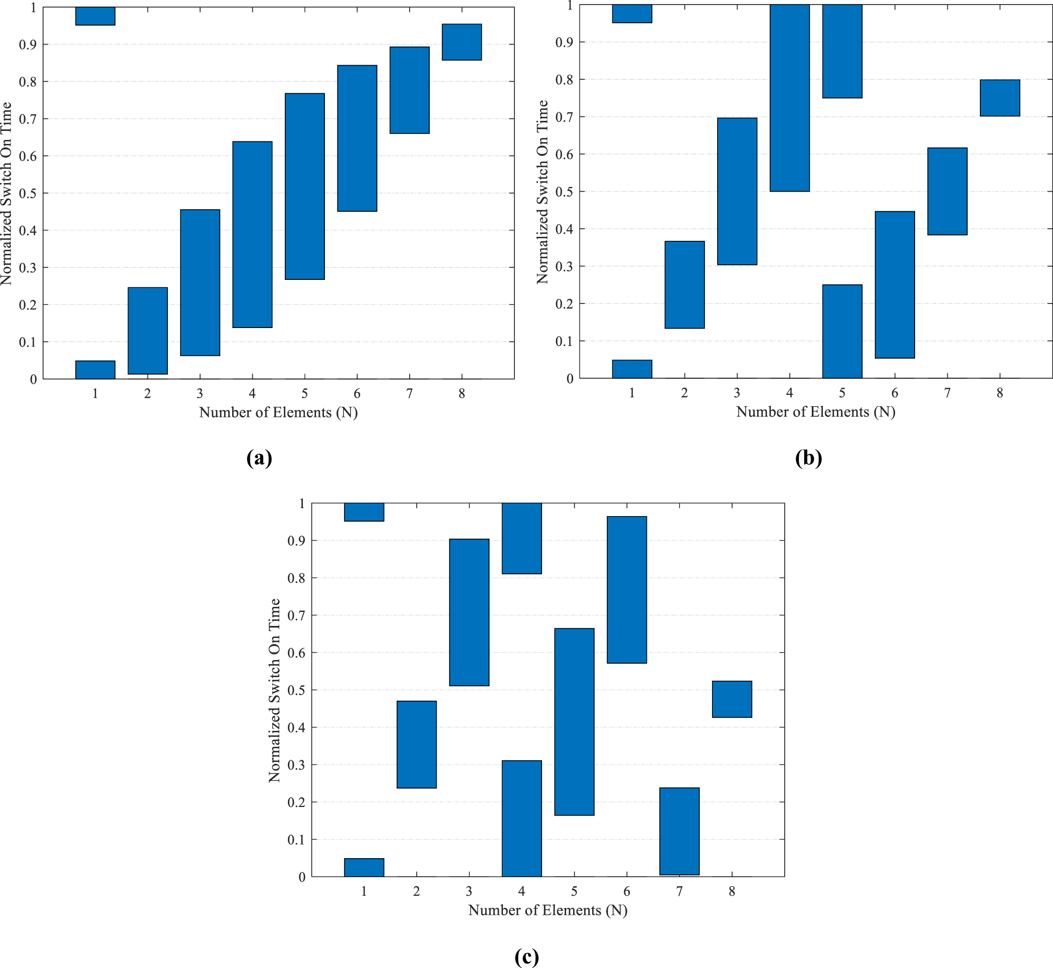
 $m = \pm 1$). To check the adaptiveness of the proposed beam scanner, the first negative and first positive harmonics are also steered toward 60°, 45°, and 120°, 135° in Cases 2 and 3, respectively. The optimal time schemes for all different pairs of scanned beams are given in Fig. 3(a), (b), and (c). The sidelobe-canceller scanning patterns generated with the optimal switching schemes are shown in Fig. 4(a), (b), and (c). In Fig. 3(a), the beam scanner is designed to scan the first harmonics to 75° and 105°, and the corresponding radiation characteristics, presented in Fig. 4(a), shows that the goal is achieved by pointing the first negative harmonics at 74.89° and the first positive harmonics at 105.11°. Similarly, the desired goals of Case 2, with scanned beams toward 60° and 120°, are also achieved by the optimal time scheme presented in Fig. 3(b). The scanned beams are pointed at 60.11° and 119.89°, as shown in Fig. 4(b). In Case 3, the scanning patterns at 45° and 135° are also achieved with the quantum-inspired optimal time scheme given in Fig. 3(c), and the corresponding scanned patterns are validated in Fig. 4(c).
Optimized sidelobe cancelling beamforming time schemes for (a) ±15°, (b) ±30°, and (c) ±45° scanned beams.

Figure 3 Long description
The image A showing a bar graph with the horizontal axis labeled Number of Elements (N) and tick labels 1, 2, 3, 4, 5, 6, 7, 8. The vertical axis is labeled Normalized Switch On Time with a range from 0 to 1. Bars are shown at each element number, each bar spanning a vertical interval. The visible bar intervals are: N equals 1 spans about 0.95 to 1.00 and about 0.00 to 0.05; N equals 2 spans about 0.00 to 0.25; N equals 3 spans about 0.05 to 0.45; N equals 4 spans about 0.15 to 0.65; N equals 5 spans about 0.27 to 0.77; N equals 6 spans about 0.45 to 0.85; N equals 7 spans about 0.65 to 0.90; N equals 8 spans about 0.88 to 0.97. The intervals generally shift upward as N increases. The image B showing a bar graph with the horizontal axis labeled Number of Elements (N) and tick labels 1, 2, 3, 4, 5, 6, 7, 8. The vertical axis is labeled Normalized Switch On Time with a range from 0 to 1. Bars are shown at each element number, each bar spanning a vertical interval. The visible bar intervals are: N equals 1 spans about 0.95 to 1.00 and about 0.00 to 0.05; N equals 2 spans about 0.13 to 0.36; N equals 3 spans about 0.30 to 0.70; N equals 4 spans about 0.50 to 1.00; N equals 5 spans about 0.00 to 0.25 and about 0.75 to 1.00; N equals 6 spans about 0.05 to 0.45; N equals 7 spans about 0.38 to 0.62; N equals 8 spans about 0.70 to 0.80. The intervals include both low and high ranges, with a full-height interval at N equals 4 and two separated intervals at N equals 5. The image C showing a bar graph with the horizontal axis labeled Number of Elements (N) and tick labels 1, 2, 3, 4, 5, 6, 7, 8. The vertical axis is labeled Normalized Switch On Time with a range from 0 to 1. Bars are shown at each element number, each bar spanning a vertical interval. The visible bar intervals are: N equals 1 spans about 0.95 to 1.00 and about 0.00 to 0.05; N equals 2 spans about 0.23 to 0.47; N equals 3 spans about 0.50 to 0.90; N equals 4 spans about 0.00 to 0.30 and about 0.80 to 1.00; N equals 5 spans about 0.15 to 0.67; N equals 6 spans about 0.57 to 0.97; N equals 7 spans about 0.00 to 0.23; N equals 8 spans about 0.43 to 0.52. The intervals vary across N, including separated intervals at N equals 4 and a low interval at N equals 7. Across A, B and C, the axes and element numbering are the same. A shows mostly upward-shifting intervals with increasing N. B and C show more mixed placement of intervals across the 0 to 1 range, including separated intervals at specific N values.
Optimized time-modulated beam scanning patterns with (a) ±15°, (b) ±30°, and (c) ±45° scanned beams.

Figure 4 Long description
The image A showing a polar plot with the text “Normalized Pattern (dB)”. Angle labels around the circle run from 0 to 360 in steps of 15. Radial tick labels shown along the left side read minus 10, minus 20, minus 30, minus 40, minus 50 and minus 60. A legend lists three curves: “Main Beam”, “Positive Harmonic” and “Negative Harmonic”. Two callouts near the top mark “C2 74.9” and “C1 105.1”. The “Main Beam” curve forms a tall lobe centered at 90. The “Positive Harmonic” curve forms a tall lobe near 105.1. The “Negative Harmonic” curve forms a tall lobe near 74.9. The image B showing a polar plot with the text “Normalized Pattern (dB)”. Angle labels around the circle run from 0 to 360 in steps of 15. Radial tick labels shown along the left side read minus 10, minus 20, minus 30, minus 40, minus 50 and minus 60. A legend lists three curves: “Main Beam”, “Positive Harmonic” and “Negative Harmonic”. Two callouts near the top mark “C2 60.1” and “C1 119.9”. The “Main Beam” curve forms a tall lobe centered at 90. The “Positive Harmonic” curve forms a tall lobe near 119.9. The “Negative Harmonic” curve forms a tall lobe near 60.1. The image C showing a polar plot with the text “Normalized Pattern (dB)”. Angle labels around the circle run from 0 to 360 in steps of 15. Radial tick labels shown along the left side read minus 10, minus 20, minus 30, minus 40, minus 50 and minus 60. A legend lists three curves: “Main Beam”, “Positive Harmonic” and “Negative Harmonic”. Two callouts near the top mark “C2 45” and “C1 135”. The “Main Beam” curve forms a tall lobe centered at 90. The “Positive Harmonic” curve forms a tall lobe near 135. The “Negative Harmonic” curve forms a tall lobe near 45.
The SLLs for the main beams, created along with the scanned beams, are suppressed to −34.8 dB, which shows an impressive improvement over the −13 dB SLL of the uniform array pattern (without optimizing  ${\xi _n}$). The SLLs of the first harmonics are also reduced to −22.8 dB, which provides convincing performance against the targeted objective of −20 dB
 $\widetilde {SLL}$ for interference rejection. Only the central pattern and the first harmonic patterns are exploited to achieve the desired beam-scanning objectives. To show that the optimized beamformer creates power-efficient beam-scanning radiating patterns, all higher-harmonic beams, except the first, are also reduced. The higher-order harmonics are suppressed as an effect of the second part of the constructed objective function, and the radiated power in higher sidebands up to 10 harmonics is calculated by using the closed-form sideband power equation derived in equation (22). The main beam and the first harmonics consume the largest portions of the total radiated power, i.e., 39.9% and 20.8%, respectively. The radiation power efficiency of the scanned patterns in the time-modulated sidelobe canceller beam scanner is 81.5%, and the total wasted power in higher harmonics is 18.5%. The other radiation properties, such as the half-power beam widths (HPBWs) of the main beams, are reported as 17.4° for all three cases. The HPBWs for the ±15°, ±30°, and ±45° scanned beams of all the three cases are reported as 16.4°, 18.5°, and 23.6°, respectively. The directivities for all the cases are measured as 8.5 dB. The analysis shows that an efficient time-modulated sidelobe-canceller beam scanner is designed in this research to address the much-needed radiation performance requirements for radars. The SPST RF switches used to implement the proposed switching scheme for beam-scanning applications also incur losses in a practical scenario, depending on the ON and OFF timings of the switches. The RF switching efficiency for SPST switches can be calculated as the ratio of the sum of the total ON time to the overall ON and OFF time within the modulation period [Reference Chakraborty, Ram and Mandal27]. The RF switching efficiency for beam scanning is calculated as 61.2%.
Single-point time-modulated jammer
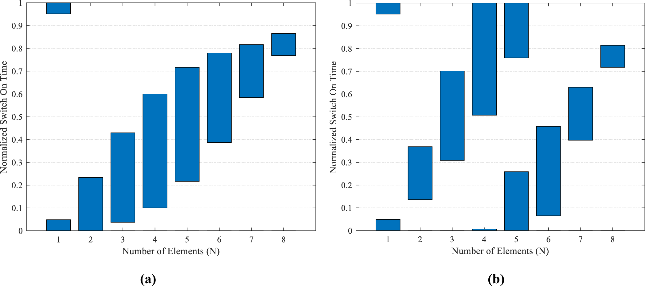
The adaptability of the time-modulated beamformer is further tested to meet the advanced radar requirements, such as steering the strategic nulls toward jammers. The idea is to point a zero-signal space into the angular region so that interfering signals in this region can be blocked. The normalized time scheme for the beamformer is designed to place single nulls by scanning the first-harmonic beams of the 8-element array for jamming mitigation. The first case of a single-point jammer with the first harmonics is targeted by producing zero-signal regions at 40° and 140°. Similarly, the second case of a single-point jammer aims to place single nulls at 60° and 120° using the symmetric first-order harmonics on both sides of the main beam pattern. In Case 1, the optimal time scheme for the proposed single-point jamming beamformer is aimed to place null points at 40° and 140°, as shown in Fig. 5(a), and the optimal pulse scheme for the second case for placing nulls toward 60° and 120°, is depicted in Fig. 5(b). The corresponding radiation patterns for a single-point anti-jammer are shown in Figs. 6 and 7. In Fig. 6(a), the first positive harmonic is scanned such that a deep null of −98.5 dB is obtained at 40°. Similarly, the first negative harmonic beam also creates a deep null of the same magnitude at 140°, given in Fig. 6(b). For the second case, the single-point jamming beamformer produces the zero-signal regions by placing deep nulls with −110 dB magnitude at 60° and 120° using the first positive and first negative harmonic beam patterns. The single-point jamming performances of Case 2 with the positive and negative harmonic responses are given in Fig. 7(a) and (b), respectively. The main beams are unaltered in the broadside direction. In addition to that, the same level of SLLs, i.e., −34.8 dB and −22.8 dB, is also maintained for the main beam and harmonic beams, respectively. The radiated power in the main beam pattern is 39.9%, and the first harmonic beams consume 20.8% power. The directivities for all the cases are reported as 8.5 dB. The RF switching efficiency for the SPST configurations proposed for the time-modulated single-point jammer is reported as 61.2%. The radiation patterns simulated using MATLAB software are also cross-validated against the CST Studio-based results for the 8-element dipole antenna arrays. The outcomes have shown close resemblance for the single-point time-modulated anti-jammer application. The proposed sidelobe-canceller beamformer performance for the single-point jammer shows much-needed adaptability and improved reception of the intended signals by blocking the unintended ones.
Optimized single-point jammer time schemes for placing deep nulls at (a) 40°, 140°, and (b) 60°, 120°.

Jamming with deep nulls at (a) 40° using the positive harmonics and (b) 140° using the negative harmonics.

Figure 6 Long description
The image A showing a line graph with the y-axis labeled Normalized Power Pattern (decibel) and the x-axis labeled Angle of Arrival (Degree). The x-axis runs from 0 to 180 with labeled ticks at 0, 20, 40, 60, 80, 100, 120, 140, 160, 180. The y-axis runs from 0 to minus 100 with labeled ticks at 0, minus 10, minus 20, minus 30, minus 40, minus 50, minus 60, minus 70, minus 80, minus 90, minus 100. A legend lists four series: Main Beam (MATLAB), Positive Harmonic (MATLAB), Main Beam (CST), Positive Harmonic (CST). The Main Beam (MATLAB) curve reaches about 0 decibel near 90 degrees, then drops with multiple narrow nulls. Visible deep nulls occur near 40 degrees, near 60 degrees, near 120 degrees, near 140 degrees and near 180 degrees, with minima reaching close to minus 100 decibel at some of these angles. The Positive Harmonic (MATLAB) curve reaches about 0 decibel near 100 degrees and shows narrow nulls near about 40 degrees, about 60 degrees, about 90 degrees, about 120 degrees, about 150 degrees and about 180 degrees, with several minima extending well below minus 60 decibel and some approaching minus 100 decibel. The Main Beam (CST) and Positive Harmonic (CST) curves are drawn with dotted styling and follow similar shapes to their corresponding MATLAB curves, including peaks near about 90 degrees and about 100 degrees and multiple narrow nulls at similar angles. The image B showing a line graph with the y-axis labeled Normalized Power Pattern (decibel) and the x-axis labeled Angle of Arrival (Degree). The x-axis runs from 0 to 180 with labeled ticks at 0, 20, 40, 60, 80, 100, 120, 140, 160, 180. The y-axis runs from 0 to minus 100 with labeled ticks at 0, minus 10, minus 20, minus 30, minus 40, minus 50, minus 60, minus 70, minus 80, minus 90, minus 100. A legend lists four series: Main Beam (MATLAB), Negative Harmonic (MATLAB), Main Beam (CST), Negative Harmonic (CST). The Main Beam (MATLAB) curve reaches about 0 decibel near 90 degrees and includes multiple narrow nulls, including dips near about 40 degrees, about 60 degrees, about 120 degrees, about 140 degrees and about 180 degrees, with some minima approaching minus 100 decibel. The Negative Harmonic (MATLAB) curve reaches about 0 decibel near 80 degrees and shows narrow nulls near about 30 degrees, about 100 degrees, about 120 degrees, about 140 degrees and about 180 degrees, with several minima below minus 60 decibel and some approaching minus 100 decibel. The Main Beam (CST) and Negative Harmonic (CST) curves are drawn with dotted styling and follow similar shapes to their corresponding MATLAB curves, including the main peak near about 90 degrees and the harmonic peak near about 80 degrees, with nulls at similar angles.
Jamming with deep nulls at (a) 60° using the positive harmonics and (b) 120° using the negative harmonics.

Figure 7 Long description
The image A showing a line graph with two solid curves and two dotted curves. The x-axis is labeled Angle of Arrival (Degree), ranging from 0 to 180 with tick marks at 0, 20, 40, 60, 80, 100, 120, 140, 160 and 180. The y-axis is labeled Normalized Power Pattern (dB), ranging from 0 to minus 110 with tick marks every 10. The legend lists Main Beam (MATLAB), Positive Harmonic (MATLAB), Main Beam (CST) and Positive Harmonic (CST). The solid main-beam curve rises from about minus 110 at 0 degrees to near 0 around 90 degrees, then falls back toward about minus 110 by 180 degrees, with multiple narrow dips between about 30 and 150 degrees that reach roughly between minus 60 and minus 90. The solid positive-harmonic curve is around minus 25 near 0 degrees, has several narrow dips between about 30 and 100 degrees including a very deep dip near 60 degrees reaching about minus 110, then rises to near 0 around 120 degrees and falls again with a narrow dip near about 150 degrees reaching roughly minus 70, ending near about minus 25 at 180 degrees. The dotted main-beam curve follows a similar arch shape to the solid main-beam curve, with a lower level around the mid angles and a deep drop near 180 degrees. The dotted positive-harmonic curve follows the solid positive-harmonic curve shape, including a deep dip near 60 degrees. The image B showing a line graph with two solid curves and two dotted curves. The x-axis is labeled Angle of Arrival (Degree), ranging from 0 to 180 with tick marks at 0, 20, 40, 60, 80, 100, 120, 140, 160 and 180. The y-axis is labeled Normalized Power Pattern (dB), ranging from 0 to minus 110 with tick marks every 10. The legend lists Main Beam (MATLAB), Negative Harmonic (MATLAB), Main Beam (CST) and Negative Harmonic (CST). The solid main-beam curve rises from about minus 110 at 0 degrees to near 0 around 90 degrees and falls back toward about minus 110 by 180 degrees, with multiple narrow dips between about 30 and 150 degrees reaching roughly between minus 60 and minus 90. The solid negative-harmonic curve is around minus 25 near 0 degrees, rises to near 0 around 60 degrees, then drops with several narrow dips between about 80 and 150 degrees including a very deep dip near 120 degrees reaching about minus 110 and then rises again toward about minus 25 by 180 degrees. The dotted main-beam curve follows the solid main-beam curve shape. The dotted negative-harmonic curve follows the solid negative-harmonic curve shape, including the deep dip near 120 degrees.
Sectorized time-modulated jammer
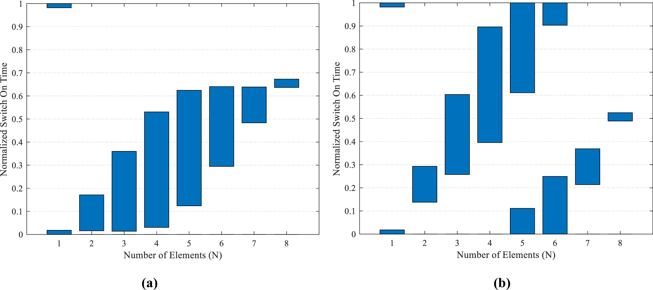
The idea of a time-modulated sidelobe-canceller jammer is further expanded in this section by proposing an adaptable beamformer to suppress interfering signals over a broad region or sector, rather than placing a deep null at a particular point. Two different cases of sectorized jamming are addressed in this research, where Case 1 deals with sectorized anti-jamming in the regions 0° to 65° and 115° to 180° using the first positive and first negative harmonic beams, respectively. In Case 2, the sectorized jamming is aimed to suppress signals in the regions 40° to 80° and 100° to 140° using first-order harmonics. The angular sectors are intended to suppress  $\widetilde {SLL}$s below −30 dB for jamming mitigation. The quantum-optimized time schemes for both cases are shown in Fig. 8(a) and (b). The corresponding sectorized jamming patterns for Case 1 with positive and negative harmonics are presented in Fig. 9(a) and (b). The first positive harmonics shown in Fig. 9(a) indicates that a broad sector from 0° to 68° is suppressed below −30 dB with a deep null of −99.6 dB at 45°. Similarly, the first negative harmonics in Fig. 9(b) provides sectorized jamming in the region of 112° to 180°, where the entire sector is suppressed below −30 dB, with a symmetric deep null at 135°. For Case 2, the first positive harmonics shown in Fig. 10(a) produce a sectorized jamming in the region from 35° to 80°, lowering all the responses in this region below −30 dB with a deep null of −96.9 dB pointed at 60°. The symmetric harmonic patterns given in Fig. 10(b) also show similar sectorized jamming performance in the region of 100° to 145° by pointing a deep null of the same magnitude at 120°. The SLLs of the main beam and first harmonic beams are suppressed as −59.8 and −26.5 dB, which shows a convincing performance over the targeted objective of −20 dB
 $\widetilde {SLL}$ for interference rejection. The directivities of the array in both cases are reported as 8.2 dB. The sectoral jammer also shows efficient power utilization, with 38.8% and 19.9% of the power consumed by the main beam and each of the first-harmonic patterns, respectively, in Case 1. The total power efficiency for the sectorized jamming application in Case 1 is 78.6%, and the power wasted in higher harmonics is 21.4%. In Case 2, the main beam and the first side beams accounts for 37.8% and 19.5% of the total radiated power, respectively. The total power efficiency is measured as 76.8%, and the power wasted in higher harmonics is 23.2%. The power utilized in desired patterns and wasted in higher-order harmonics for all the objectives is shown in Fig. 11. The RF switching efficiency for the SPST configurations proposed in time-modulated sectorized jammer is reported as 51.8%. The radiation patterns simulated in MATLAB are also cross-validated against CST Studio-based results for the 8-element dipole antenna arrays. The outcomes have shown close resemblance for the sectorized time-modulated anti-jammer application.
Optimized sectoral jammer timings to suppress (a) 0° to 65° and 115° to 180°, (b) 40° to 80° and 100° to 140°.

Sectoral jamming patterns to suppress (a) 0° to 65° and (b) 115° to 180° using positive and negative harmonics.

Figure 9 Long description
The image A showing a line graph with the y-axis labeled Normalized Power Pattern (decibel) and the x-axis labeled Angle of Arrival (Degree). The x-axis runs from 0 to 180 with labeled ticks at 0, 20, 40, 60, 80, 100, 120, 140, 160, 180. The y-axis runs from 0 to minus 110 with labeled ticks at 0, minus 10, minus 20, minus 30, minus 40, minus 50, minus 60, minus 70, minus 80, minus 90, minus 100, minus 110. A legend lists four series: Main Beam (MATLAB), Positive Harmonic (MATLAB), Main Beam (CST), Positive Harmonic (CST). The Main Beam (MATLAB) curve rises to about 0 near 90 degrees, then drops with multiple narrow nulls below minus 80 between about 120 and 160 degrees and additional narrow nulls below minus 80 between about 20 and 60 degrees. The Main Beam (CST) curve follows a similar shape, with a peak near 90 degrees around 0 and multiple narrow nulls below minus 80 in the same angle regions. The Positive Harmonic (MATLAB) curve is around minus 30 at 0 degrees, decreases to below minus 90 near about 45 degrees, rises to near 0 around 100 degrees, then decreases toward about minus 55 by 180 degrees, with a narrow deep notch near about 80 degrees reaching below minus 60. The Positive Harmonic (CST) curve follows a similar path, with a deep minimum near about 45 degrees below minus 90, a peak near about 100 degrees near 0 and a decline toward the right side. The image B showing a line graph with the y-axis labeled Normalized Power Pattern (decibel) and the x-axis labeled Angle of Arrival (Degree). The x-axis runs from 0 to 180 with labeled ticks at 0, 20, 40, 60, 80, 100, 120, 140, 160, 180. The y-axis runs from 0 to minus 110 with labeled ticks at 0, minus 10, minus 20, minus 30, minus 40, minus 50, minus 60, minus 70, minus 80, minus 90, minus 100, minus 110. A legend lists four series: Main Beam (MATLAB), Negative Harmonic (MATLAB), Main Beam (CST), Negative Harmonic (CST). The Main Beam (MATLAB) curve peaks near 90 degrees around 0, then drops with multiple narrow nulls below minus 80 between about 120 and 160 degrees and additional narrow nulls below minus 80 between about 20 and 60 degrees. The Main Beam (CST) curve follows a similar shape with a peak near 90 degrees around 0 and similar narrow null locations. The Negative Harmonic (MATLAB) curve rises from about minus 55 at 0 degrees to near 0 around 80 to 90 degrees, then drops sharply to a deep minimum below minus 60 near about 100 degrees, rises to around minus 25 near about 115 degrees, then drops again to below minus 90 near about 140 degrees and rises toward about minus 30 by 180 degrees. The Negative Harmonic (CST) curve follows a similar pattern, including a peak near about 80 to 90 degrees near 0 and a deep minimum near about 140 degrees below minus 90.
Sectoral jamming patterns to suppress (a) 40° to 80° and (b) 100° to 140° using positive and negative harmonics.

Figure 10 Long description
The image A showing a line graph with the y-axis labeled Normalized Power Pattern (decibel) and the x-axis labeled Angle of Arrival (Degree). The x-axis runs from 0 to 180 with labeled ticks at 0, 20, 40, 60, 80, 100, 120, 140, 160, 180. The y-axis runs from 0 to minus 110 with labeled ticks at 0, minus 10, minus 20, minus 30, minus 40, minus 50, minus 60, minus 70, minus 80, minus 90, minus 100, minus 110. A legend lists four series: Main Beam (MATLAB), Positive Harmonic (MATLAB), Main Beam (CST), Positive Harmonic (CST). The main-beam curves form a broad peak near 100 degrees, reaching close to 0 decibel, then drop steeply on both sides. Multiple narrow nulls appear on the main-beam curves, including several dips below minus 80 decibel between about 20 and 60 degrees and several dips below minus 80 decibel between about 120 and 160 degrees. The positive-harmonic curves rise to a peak near 120 degrees close to 0 decibel, with a sharp narrow dip near about 100 degrees reaching roughly minus 70 decibel and another sharp narrow dip near about 140 degrees reaching roughly minus 70 decibel. A shaded vertical band spans approximately 60 to 90 degrees. The image B showing a line graph with the y-axis labeled Normalized Power Pattern (decibel) and the x-axis labeled Angle of Arrival (Degree). The x-axis runs from 0 to 180 with labeled ticks at 0, 20, 40, 60, 80, 100, 120, 140, 160, 180. The y-axis runs from 0 to minus 110 with labeled ticks at 0, minus 10, minus 20, minus 30, minus 40, minus 50, minus 60, minus 70, minus 80, minus 90, minus 100, minus 110. A legend lists four series: Main Beam (MATLAB), Negative Harmonic (MATLAB), Main Beam (CST), Negative Harmonic (CST). The main-beam curves form a broad peak near 80 degrees, reaching close to 0 decibel, then drop steeply on both sides. Multiple narrow nulls appear on the main-beam curves, including several dips below minus 80 decibel between about 20 and 60 degrees and several dips below minus 80 decibel between about 120 and 160 degrees. The negative-harmonic curves rise to a peak near 60 degrees close to 0 decibel, then fall and include a sharp narrow dip near about 90 degrees reaching roughly minus 70 decibel. Another sharp narrow dip appears near about 120 degrees reaching roughly minus 100 decibel. A shaded vertical band spans approximately 120 to 150 degrees.
Power consumed by the main beam, first harmonics, and higher harmonics patterns for (a) Sidelobe-canceller beamformer, (b) Beam scanner, (c) Sectoral anti-jammer Case 1, and (d) Sectoral anti-jammer Case 2.

Figure 11 Long description
The image contains four bar graphs comparing radiated power percent by harmonic order for different beamforming cases. All graphs share the same axes: the horizontal axis labeled Harmonics (m) from 0 to 10 and the vertical axis labeled Radiated Power (percent) from 0 to 45. The legend indicates Power Utilized. Graph (a) represents the sidelobe-canceller beamformer. Key values are 39.9 percent for harmonic 0 and 20.8 percent for harmonic 1. Harmonics 2 to 10 show minimal power, decreasing progressively. Graph (b) represents the beam scanner. It mirrors graph (a) with 39.9 percent at harmonic 0 and 20.8 percent at harmonic 1. Harmonics 2 to 10 remain low. Graph (c) represents sectoral anti-jammer Case 1. It shows 38.8 percent at harmonic 0 and 19.9 percent at harmonic 1. Harmonics 2 to 10 are slightly higher than in (a) and (b) but still low. Graph (d) represents sectoral anti-jammer Case 2. It displays 37.8 percent at harmonic 0 and 19.5 percent at harmonic 1. Harmonics 2 to 10 are similar to (c). Across all graphs, most power is concentrated in harmonics 0 and 1, with harmonics 2 to 10 contributing minimally. The green bars represent fundamental harmonics, while red bars indicate higher harmonics. Graphs (a) and (b) are identical, while (c) and (d) show slightly reduced power at harmonics 0 and 1.
The comparison of the proposed beamformer outcomes with other state-of-the-art works is also presented in Table 1. The SLL of the main beam pattern has improved to −59.8 dB. The SLL for the anti-jamming first-harmonic beams is −26.5 dB, compared to the best-reported result of −23.8 dB. The overall power efficiency has also shown superior performance with 78.6% compared to 71.28% reported in Table 1. From detailed analysis, it is proven that an efficient and adaptive sidelobe-canceller beamformer is designed in this research which is capable of electronic beam scanning, sidelobe cancellation, placing single nulls for single-point jamming, and suppression of signals for sectoral jamming mitigation useful for radars.
Comparison of the proposed sidelobe cancelling time-modulated beamformer with other contemporary works

Table 1 Long description
The table compares multiple published time modulated beamforming approaches using sidelobe level in decibels for the main component and the first side components, plus power split and efficiency metrics where reported. The proposed beamformer reports a main component sidelobe level of minus 59.8 dB and first side component sidelobe level of minus 26.5 dB, with 38.8% power in the main component, 19.9% in the first side components, 78.6% power efficiency, and 21.4% wasted power. Earlier Poli results cluster near minus 21 to minus 22 dB for the main component and minus 20 dB for the first side components, with efficiencies around 69.7% to 71.9% and wasted power around 28.1% to 30.9%. Other works report sidelobe levels only: Tan 2021 lists minus 20 dB main and minus 23.6 dB first side; Gassab 2019 ranges from minus 30 dB main with minus 12 dB first side to minus 18.9 dB main with minus 23.8 dB first side; Ram 2021 cases range from minus 14.9 to minus 18.2 dB for both components; Bhattacharya 2017 reports about minus 18.3 and minus 18.4 dB in one case and minus 22.4 and minus 22.2 dB in another. Overall, the proposed method is the clear outlier with much lower main component sidelobes and higher reported efficiency than the few studies that provide power metrics. Many entries lack power and efficiency values, so comparisons on energy distribution and efficiency are limited to the rows with available data.
* C1, C2, C3, C4 – Different Cases; *Na – Not available
Conclusion
The research proposes the design of an efficient time-modulated sidelobe-canceller beamformer array for advanced radar applications by emphasizing and exploring the electronic beam scanning, null placing, and jamming mitigation capabilities. Scanning patterns toward prespecified directions is a crucial requirement for modern radars, enabling the accurate tracking of an object or intended signals. The associated challenges, such as sidelobe suppression while maintaining the radiation efficiencies of the beam patterns, are also addressed in this research. Furthermore, optimal time-scheme frameworks have been developed to provide jamming mitigation characteristics in the desired directions. A complete mathematical model of the switching schemes required to achieve the objectives in an 8-element time-modulated array is proposed. In addition to that, the mathematical modeling of the shifted switching scheme, responsible for a cumulative phase divergence performance, is also presented in this research. The proposed sidelobe-canceller beamformer achieves decent scanning coverage of around 90° in the broadside direction. The simultaneous harmonic beams of the time-modulated beamformer also ensure good sidelobe suppression properties by maintaining below −30 dB sidelobe levels (SLLs) for all the proposed applications. The SLLs of the harmonic patterns are also suppressed along with the main beam, suggesting a simple beamforming network that can affect all harmonics and the desired beams simultaneously. The electronic beam-scanning performance shows that the first negative and positive harmonics are utilized to scan at multiple prespecified directions, including 45°, 60°, 75°, 105°, 120°, and 135°. The broad scan coverage from 45° to 135°, with sidelobes below −34.8 dB and −22.8 dB for interference rejection, is useful for scanning radars. Further, single-point jammers are targeted by placing null points in the angle of arrival, and the results show the jamming performance of the proposed single-point jammers at 40°, 60°, 120°, and 140° with desired sidelobe suppression. The idea is further expanded to sectorized jamming, where specific regions such as 0° to 65°, 40° to 80°, 100° to 140°, and 115° to 180° are targeted to suppress signals below the desired level blocking transmission or reception in those sectors. The overall sidelobes of the main beam and the harmonic beams are also lowered to −59.8 dB and −26.5 dB. The radiation power efficiencies of all the proposed applications also show that around 80% of the power is utilized for scanning and jamming applications. The proposed results are also compared with the state-of-the-art research to show their superior performance. This research proposes and explores time-modulated beamforming antenna arrays capable of simultaneous electronic beam scanning and jamming mitigation, with sidelobe reduction characteristics.
Data availability statement
No new data are created or analyzed during the work. The sharing of data is not applicable for this article.
Competing interests
The authors hereby declare that they do not have any competing financial or personal interests.