1 Introduction
Bubble columns are widely employed in industry because they can offer excellent heat and mass transfer characteristics without requiring any additional mechanical stirring. They are conceptually simple: a gas is sparged at the bottom of a liquid-filled vessel and the bubbles rise under the effect of buoyancy. High transfer rates can then be attained owing to the increased contact area between the gas and the liquid phases, and to the liquid agitation induced by the bubbles’ motion. Since a reliable prediction of bubble residence time and available interfacial area is crucial for an accurate and successful design of industrial columns, the understanding of bubble flow dynamics is essential.
In this context, a fundamental problem is the accurate prediction of the average bubble rise velocity in a statistically homogeneous buoyancy-driven flow of monodisperse bubbles, with the intention of using the results to systems with weak confinement and/or large-scale gradients. The average bubble rise velocity relative to the average velocity of the entire suspension is termed herein the drift velocity and the magnitude of the drift velocity is denoted by
 $U$
. In the dilute limit (wherein the bubble volume fraction is vanishingly small), if no clustering occurs, bubbles behave as if they were isolated, and the drift velocity approaches the terminal velocity
 $U_{0}$
of a single bubble in unbounded liquid under otherwise the same conditions, for which a number of correlations are available (Clift, Grace & Weber Reference Clift, Grace and Weber1978; Loth Reference Loth2008). As volume fraction increases,
 $U$
generally departs from
 $U_{0}$
. We therefore define
 $G(\unicode[STIX]{x1D719})=U/U_{0}$
, where
 $\unicode[STIX]{x1D719}$
is the gas volume fraction; the dependencies of
 $G$
on various other dimensionless groups (termed herein as ‘flow conditions’) are suppressed in the notation for
 $G$
for brevity, but are not ignored.
A common form of the dependency on volume fraction used in empirical correlations is the Richardson–Zaki expression
 $G(\unicode[STIX]{x1D719})=(1-\unicode[STIX]{x1D719})^{n}$
(Richardson & Zaki Reference Richardson and Zaki1954; Ishii & Zuber Reference Ishii and Zuber1979), where
 $n$
is an empirical parameter that depends on flow conditions. Various experiments have been carried out previously to determine
 $G(\unicode[STIX]{x1D719})$
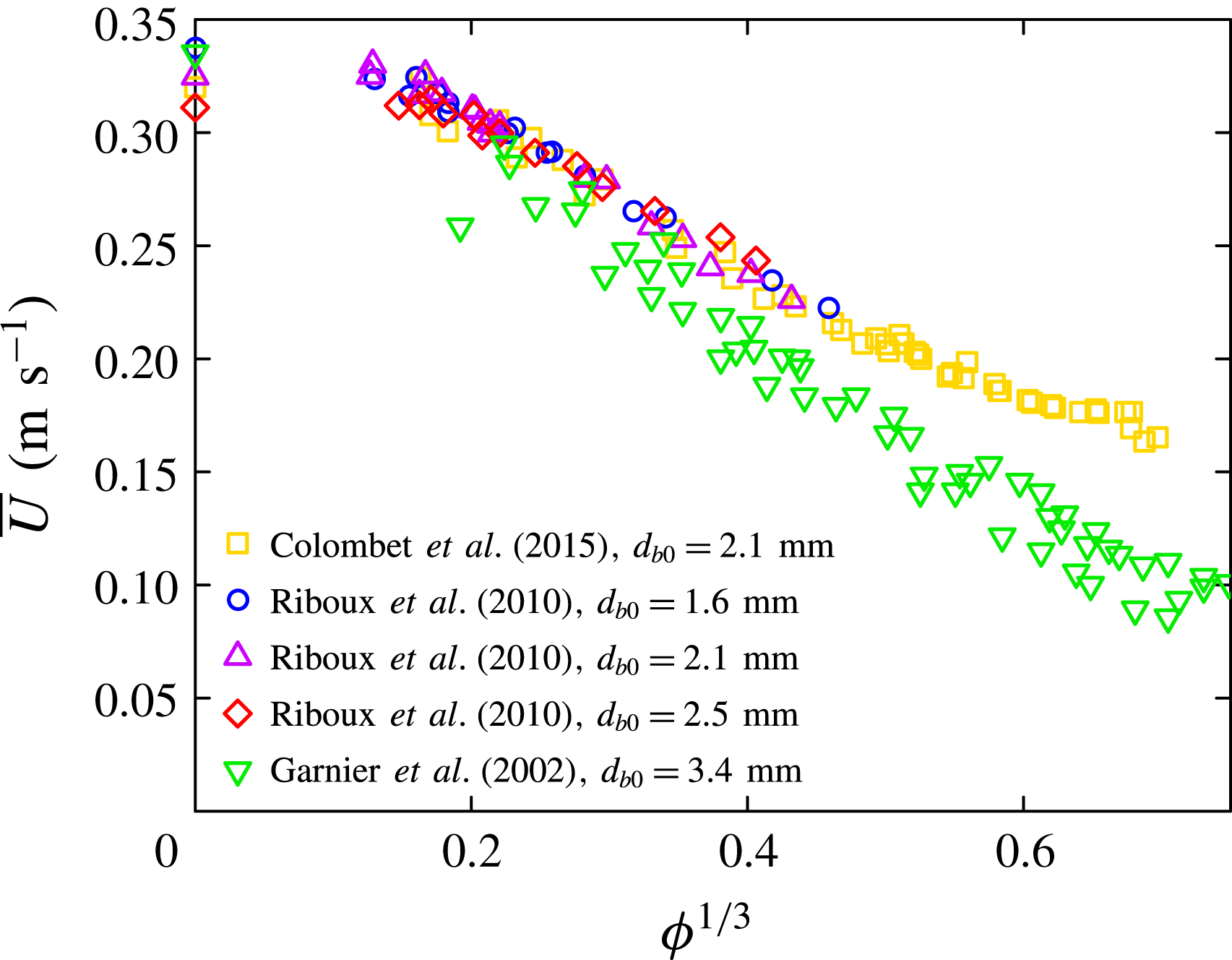
by injecting bubbles of millimetric size in a vertical column filled with clean water. In their respective experiments, Zenit, Koch & Sangani (Reference Zenit, Koch and Sangani2001) found that their measurements could be approximately described by the Richardson–Zaki formula with exponent
 $n=2.8$
, Garnier, Lance & Marié (Reference Garnier, Lance and Marié2002) obtained instead
 $G(\unicode[STIX]{x1D719})=1-\unicode[STIX]{x1D719}^{1/3}$
and Colombet et al. (Reference Colombet, Legendre, Risso, Cockx and Guiraud2015) fitted their data by
 $G(\unicode[STIX]{x1D719})=(0.28+0.72\exp (-15\unicode[STIX]{x1D719}))^{1/2}$
. Experimental complexities may have arisen that could explain these differences. For example, it is challenging to purify water of surfactants, to rule out wall effects and to obtain a truly monodisperse suspension. A main inconvenience is that usually the bubble diameter cannot be kept constant if the volume fraction is changed, and the terminal velocity (and shape) of a single bubble strongly depends on the bubble size (Clift et al.
Reference Clift, Grace and Weber1978). This renders difficult disentangling the dependency of drift velocity on hydrodynamic interactions – along with the microstructure – from that on bubble size if the latter is varied simultaneously with volume fraction.
Theoretical predictions of the drift velocity of bubbles are available for asymptotic and ideal systems. The drift (or rather, sedimentation) velocity derived by Batchelor (Reference Batchelor1972) for rigid particles in Stokes flow, wherein a uniformly random sedimenting suspension of particles is considered, has been generalized to droplets and bubbles, yielding
 $G(\unicode[STIX]{x1D719})=1-4.44\unicode[STIX]{x1D719}+O(\unicode[STIX]{x1D719}^{2})$
for bubbles whose viscosity can be ignored compared to that of the liquid (Keh & Tseng (Reference Keh and Tseng1992); earlier work cited therein used various approximations for the mobility matrix). This linear correction includes a contribution
 $-\unicode[STIX]{x1D719}$
due to the back flow induced by the bubble motion, to maintain the mixture velocity of the entire suspension. It also includes a contribution
 $-3\unicode[STIX]{x1D719}$
from a volume-exclusion effect: a test bubble drags some liquid along with it which is compensated by a downflow further away; other bubbles cannot access the fluid in the direct vicinity of the test bubble (as this would require bubbles to overlap) and therefore sample a net fluid downflow (see Batchelor (Reference Batchelor1972) and for the application to bubbles/droplets see Wacholder (Reference Wacholder1973), albeit that an approximation for the mobility was used by the latter). The remainder of the linear term in
 $G(\unicode[STIX]{x1D719})$
is due to near-bubble interactions.
The drift velocity strongly depends already on the microstructure in the dilute limit. If the probability of finding a particulate near a test particulate is uniform outside the excluded volume, as is appropriate for colloidal dispersions (Glendinning & Russel Reference Glendinning and Russel1982) and as is assumed in the works cited above, interactions with nearby particulates result in
 $G(\unicode[STIX]{x1D719})\sim 1-O(\unicode[STIX]{x1D719})$
, whereas for a microstructure wherein a dominant contribution comes from particulates at a distance that corresponds to the mean separation
 $(V_{p}/\unicode[STIX]{x1D719})^{1/3}$
, with
 $V_{p}$
the particulate volume, one expects
 $G(\unicode[STIX]{x1D719})=1-O(\unicode[STIX]{x1D719}^{1/3})$
(e.g. Davis & Acrivos Reference Davis and Acrivos1985). A well-known example of the latter is a microstructure wherein particulates are arranged in a regular, ordered array. For bubbles arranged in an ordered array,
 $G(\unicode[STIX]{x1D719})=1-b\unicode[STIX]{x1D719}^{1/3}+O(\unicode[STIX]{x1D719}^{2})$
, where the coefficient
 $b$
is known for several cubic arrays and the
 $O(\unicode[STIX]{x1D719})$
term cancels if the gas viscosity is ignored compared to the liquid viscosity (Sangani & Acrivos Reference Sangani and Acrivos1983; Sangani Reference Sangani1987). The microstructure is not known a priori, therefore these limiting cases of random and ordered arrays may provide the means to determine the possible magnitude of the effects of order of the microstructure.
Besides Stokes flows, a weakly viscous theory based on potential-flow interactions has also been developed (Spelt & Sangani Reference Spelt and Sangani1998). Exceptionally, the probability density function for a configuration of identical spherical bubbles is known in that case. The pair probability shows a peak around the horizontal plane and a deficit for bubbles aligned vertically, both vanishing at large separation, if the drift velocity is not small compared to bubble velocity fluctuations, as may be expected from a Bernoulli effect. The averaged drag coefficient could therefore be determined analytically in the dilute limit whilst accounting for the microstructure. In the present notation, this yielded
 $G(\unicode[STIX]{x1D719})=1-(17/8+9A/20)\unicode[STIX]{x1D719}+O(\unicode[STIX]{x1D719}^{2})$
, where
 $A$
is the ratio of
 $U^{2}$
and the root-mean-square bubble velocity; a Padé approximation for use beyond the dilute limit is presented in Spelt & Sangani (Reference Spelt and Sangani1998), and an extension for non-spherical bubbles at small
 $A$
is also available (Kushch et al.
Reference Kushch, Sangani, Spelt and Koch2002). The dependency on
 $A$
enters there because it affects the pair probability density function in that analysis, this being nearly isotropic at low
 $A$
whilst showing a preference for bubbles rising nearly side by side at large
 $A$
. Thus, in this description, the microstructure is determined from the significance of the drift velocity compared to that of bubble velocity fluctuations, the latter being the result of local inhomogeneities such as the shear rate (see Spelt & Sangani Reference Spelt and Sangani1998).
Beyond these theoretical approaches, direct numerical simulations (DNS) of unbounded buoyancy-driven flows, in the sense of resolving the full Navier–Stokes equations coupled with the bubble dynamics and deformation, have been performed in prior work for cubic domains that contain a finite number of freely moving bubbles subject to periodic boundary conditions. Conveniently, this set-up allows variation between microstructures. On the one hand, for a given volume fraction, using a large number of bubbles in the unit cell is of interest as a model of real suspensions, although convergence with number of particulates would have to be verified, since for Stokes interactions this may be slow (Phillips, Brady & Bossis Reference Phillips, Brady and Bossis1988), or a dependency on system size may even persist (Guazzelli & Hinch Reference Guazzelli and Hinch2011); in the studies cited below, typically
 $O(10)$
–
 $O(100)$
bubbles are used in a unit cell and the effect of system size is found to be small. At the other extreme, the special case of one freely rising bubble in the unit cell, one recovers a simple cubic array. We shall herein refer to this set-up with more than one bubble in the unit cell as a free array and to that with one bubble in the cell as an ordered array.
For spherical bubbles rising at low (
 $O(1)$
) Reynolds numbers, the DNS results of Esmaeeli & Tryggvason (Reference Esmaeeli and Tryggvason1998) suggest that
 $G(\unicode[STIX]{x1D719})$
for free arrays may be similar to that predicted for ordered arrays, but the system studied was concluded to be too small to draw definitive conclusions. Bunner & Tryggvason (Reference Bunner and Tryggvason2003) found that their results at moderate (
 $O(10)$
) Reynolds numbers could be represented by
 $G(\unicode[STIX]{x1D719})=1-\unicode[STIX]{x1D719}^{1/3}$
for spherical bubbles in free arrays, and a Richardson–Zaki expression with exponent
 $n=3$
for deformable bubbles, but no theoretical justification for these scalings could be offered beyond an observed difference in preferential spatial configurations of bubbles, discussed further below. Also, the expressions for
 $G(\unicode[STIX]{x1D719})$
inferred in these pioneering studies could only be fitted from just a few different values of the volume fraction comprised between 2 % and 12 % and their validity outside this range seems unclear. Further results for free arrays at moderate Reynolds numbers were obtained by Yin & Koch (Reference Yin and Koch2008), for volume fractions ranging from 1 % to 25 %, using a lattice Boltzmann method. They used
 $O(100)$
bubbles in a periodic cell, rather than
 $O(10)$
in most of the early studies cited above, and imposed a spherical shape facilitated by a force balance that included the surface integral of the traction acting on the bubble and the buoyancy force. Their results demonstrate that
 $G(\unicode[STIX]{x1D719})$
is not well fitted by the Richardson–Zaki formula, and they suggest that this is associated with the anisotropic microstructure of bubbly suspensions in this regime. Gillissen, Sundaresan & Van Den Akker (Reference Gillissen, Sundaresan and Van Den Akker2011) conducted similar simulations using a combination of lattice Boltzmann and immersed boundary methods, and obtained
 $G(\unicode[STIX]{x1D719})=1-O(\unicode[STIX]{x1D719}^{1/3})$
for spherical bubbles rising at small to moderate Reynolds number, in qualitative agreement with earlier studies (Esmaeeli & Tryggvason Reference Esmaeeli and Tryggvason1998; Bunner & Tryggvason Reference Bunner and Tryggvason2003).
From these prior studies, the microstructure, along with the drift velocity, is known to vary significantly with bubble Reynolds number and shape. For spherical bubbles rising at
 $O(100)$
Reynolds number, strong preference for horizontal alignment is observed in the simulated pair probability (Esmaeeli & Tryggvason Reference Esmaeeli and Tryggvason2005), in agreement with the trends reviewed above for the idealized potential-flow interactions. The anisotropy in microstructure is larger than that observed in the experiments of Zenit et al. (Reference Zenit, Koch and Sangani2001), possibly because of bubble deformation: indeed the simulations of Esmaeeli & Tryggvason (Reference Esmaeeli and Tryggvason2005) revealed that oblate ellipsoidal bubbles do not form horizontal rafts but instead are rather uniformly distributed. At
 $O(10)$
Reynolds number, the dynamics of bubble–bubble interactions is dominated by wake effects. A vertical pair of spherical bubbles changes its orientation to horizontal through a drafting–kissing–tumbling mechanism, resulting in preferential side-by-side alignment (Esmaeeli & Tryggvason Reference Esmaeeli and Tryggvason1999; Bunner & Tryggvason Reference Bunner and Tryggvason2002a
; Yin & Koch Reference Yin and Koch2008), whereas deformable bubbles tend to organize in vertical structures owing to the reversed lift force which attracts a bubble in the wake of its preceding neighbour (Bunner & Tryggvason Reference Bunner and Tryggvason2003). These effects decrease with decreasing Reynolds number and nearly no preference is observed at
 $O(1)$
Reynolds number (Esmaeeli & Tryggvason Reference Esmaeeli and Tryggvason1998; Cartellier & Rivière Reference Cartellier and Rivière2001).
In the DNS studies cited thus far, the microstructure is allowed to develop naturally. For use of the results in general flows, wherein microstructure can be affected by weak gradients, it is necessary to know the role of and sensitivity to the microstructure. DNS results for rising deformable bubbles in an ordered arrangement have been conducted by Sankaranarayanan et al. (Reference Sankaranarayanan, Shan, Kevrekidis and Sundaresan2002), using a lattice Boltzmann method. An empirical correlation of Richardson–Zaki form was used to represent the results for a vast range of flow regimes, albeit for
 $5\leqslant \unicode[STIX]{x1D719}\leqslant 25\,\%$
and with the reservation that the correlation does not reduce to the analytical result discussed above for creeping flows of ordered arrays.
Despite their apparent artificiality, ordered arrays of bubbles, as well as their relevance to real bubbly flows, certainly deserve further investigation. Firstly, a number of prior simulations and experiments reviewed above for
 $1\lesssim \mathit{Re}\lesssim 1000$
found a bubble rise velocity scaling as
 $\unicode[STIX]{x1D719}^{1/3}$
(Esmaeeli & Tryggvason Reference Esmaeeli and Tryggvason1998; Garnier et al.
Reference Garnier, Lance and Marié2002; Bunner & Tryggvason Reference Bunner and Tryggvason2003; Gillissen et al.
Reference Gillissen, Sundaresan and Van Den Akker2011). This scaling is the same as that obtained assuming a periodic arrangement of the bubbles, albeit under the Stokes flow approximation (Sangani & Acrivos Reference Sangani and Acrivos1983). The study of ordered arrays beyond the Stokes flow limit is therefore of fundamental interest in order to connect theoretical, numerical and experimental work. Secondly, prior experimental and numerical work on bubbly flows at moderate to high Reynolds number has shown that the magnitude of the bubble velocity fluctuations is substantially smaller than the bubble rise velocity (Zenit et al.
Reference Zenit, Koch and Sangani2001; Bunner & Tryggvason Reference Bunner and Tryggvason2002b
; Esmaeeli & Tryggvason Reference Esmaeeli and Tryggvason2005; Martinez-Mercado, Palacios-Morales & Zenit Reference Martinez-Mercado, Palacios-Morales and Zenit2007), at least when the gas volume fraction remains below approximately 10 %. This further motivates a study of a representation of bubbly suspensions by ordered arrays (zero bubble velocity fluctuations). Thirdly, only experimental investigations can assess the relevance (or lack thereof) of the ordered model to describe real bubbly suspensions. By re-examining prior experimental data (Garnier et al.
Reference Garnier, Lance and Marié2002; Martinez-Mercado et al.
Reference Martinez-Mercado, Palacios-Morales and Zenit2007; Riboux, Risso & Legendre Reference Riboux, Risso and Legendre2010; Colombet et al.
Reference Colombet, Legendre, Risso, Cockx and Guiraud2015), we will show that available measurements support the idea that ordered arrays are indeed relevant to bubbly flows of practical interest.
In this paper, we investigate the ordered and free rise of bubbles at low and moderate Reynolds numbers over a wide range of volume fractions, using DNS and analysis; the problem statement is presented in § 2 and the numerical methods in § 3. The first objective (in § 4) is to determine the connection between the DNS results and theory for dilute ordered systems and, beyond the dilute limit, the connection between the DNS results and prior work on bubble pairs, which have been studied analytically (e.g. Harper Reference Harper1970, Reference Harper1997), experimentally (Katz & Meneveau Reference Katz and Meneveau1996) and computationally (Yuan & Prosperetti Reference Yuan and Prosperetti1994; Legendre, Magnaudet & Mougin Reference Legendre, Magnaudet and Mougin2003; Hallez & Legendre Reference Hallez and Legendre2011). For that purpose, the first effects of inertia are determined analytically, and a comprehensive parametric DNS study is presented at low and moderate Reynolds number in § 4.1. The study includes ordered suspensions of strongly deformed (skirted) bubbles that have not been studied thus far. The results are summarized in a practical relation that covers a wide range of flows and reduces to analytical results in the dilute limit. In particular, the DNS and the theory in the dilute limit demonstrate that
 $G(\unicode[STIX]{x1D719})$
is not monotonic at low
 $\unicode[STIX]{x1D719}$
; Bunner & Tryggvason (Reference Bunner and Tryggvason2002a
) and Roghair et al. (Reference Roghair, Lau, Deen, Slagter, Baltussen, Van Sint Annaland and Kuipers2011) remarked that
 $G(\unicode[STIX]{x1D719})$
increases at small volume fractions, but did not investigate this further. The surprising dynamics of ordered suspensions is then investigated in § 4.2. A steady oblique rise was observed in the DNS in some cases, as a precursor to unsteady (periodic and non-periodic) behaviour. Oblique motion of two-dimensional square arrays of bubbles has been observed previously (Sankaranarayanan et al.
Reference Sankaranarayanan, Shan, Kevrekidis and Sundaresan2002; Sankaranarayanan & Sundaresan Reference Sankaranarayanan and Sundaresan2002; Theodoropoulos et al.
Reference Theodoropoulos, Sankaranarayanan, Sundaresan and Kevrekidis2004), but remains essentially unexplained. We support the existence of oblique rise for ordered suspensions with analysis in the dilute limit, and demonstrate that the inferred lift coefficient is similar to that obtained for the rise of bubble pairs. The second objective of the present work is to revisit (in § 5) arrays of free bubbles in light of these findings for ordered arrays, and to contrast and compare these two systems. In § 5.2, numerical results are presented for freely evolving bubbly suspensions at small and intermediate volume fractions and similarities with ordered systems are highlighted. These are supported by a comparison with experimental data in § 5.3. Finally, conclusions are presented in § 6.
2 Mathematical formulation
2.1 Problem statement
We consider an infinite, homogeneous, monodisperse suspension of bubbles rising under the effect of buoyancy in otherwise quiescent liquid. The density and viscosity of each fluid, as well as the surface tension, are assumed to be constant. The suspension is represented by the periodic repetition of a cubic unit cell containing a given number of bubbles. The gravity is aligned with a primary axis of the periodic array (due to the large number of parameters already involved in the problem, the influence of the orientation of gravity is not investigated here).
The behaviour of this system depends on nine parameters: the number of bubbles
 $N_{b}$
in the cell, the gas volume fraction
 $\unicode[STIX]{x1D719}$
, the gravitational acceleration
 $g$
, the bubble volume or, more conveniently, its characteristic size
 $d_{b}$
defined as the diameter of the volume-equivalent sphere and the physical properties of the two fluids, namely their densities (
 $\unicode[STIX]{x1D70C}_{d}$
,
 $\unicode[STIX]{x1D70C}_{c}$
), their viscosities (
 $\unicode[STIX]{x1D707}_{d}$
,
 $\unicode[STIX]{x1D707}_{c}$
) and the surface tension (
 $\unicode[STIX]{x1D6FE}$
). The subscripts
 $d$
and
 $c$
refer to the disperse (gaseous) and continuous (liquid) phases, respectively.
In addition to the gas volume fraction and to the number of bubbles, four independent dimensionless groups can be constructed from the remaining parameters. Two of these are the ratios of the gas density and viscosity to those of the surrounding liquid. These are usually very small and of the same order for most gas–liquid systems of practical interest. As a consequence their influence will not be investigated, and unless otherwise mentioned, these parameters will be set to
 $\unicode[STIX]{x1D70C}_{d}/\unicode[STIX]{x1D70C}_{c}=10^{-3}$
and
 $\unicode[STIX]{x1D707}_{d}/\unicode[STIX]{x1D707}_{c}=10^{-2}$
, which approximately corresponds to air bubbles in water. The last two dimensionless numbers are the Archimedes number
 $$\begin{eqnarray}\mathit{Ar}=\frac{\sqrt{\unicode[STIX]{x1D70C}_{c}|\unicode[STIX]{x1D70C}_{d}-\unicode[STIX]{x1D70C}_{c}|gd_{b}^{3}}}{\unicode[STIX]{x1D707}_{c}},\end{eqnarray}$$
or equivalently the Galilei number
 $\mathit{Ga}=\mathit{Ar}^{2}$
, and the Bond number (also known as the Eötvös number),
 $$\begin{eqnarray}\mathit{Bo}=\frac{|\unicode[STIX]{x1D70C}_{d}-\unicode[STIX]{x1D70C}_{c}|gd_{b}^{2}}{\unicode[STIX]{x1D6FE}}.\end{eqnarray}$$
The Archimedes and Bond numbers can be defined a priori, without the knowledge of the bubble velocity, and are therefore traditionally employed to describe the macroscopic conditions of buoyancy-driven bubbly flow (numerical) experiments.
At time zero, the bubbles are released from rest and start rising. The time evolution of the system is monitored through
 $\boldsymbol{U}(t)$
, defined as the average drift velocity of the bubbles and computed at any time from
 $$\begin{eqnarray}\boldsymbol{U}=\langle \boldsymbol{u}\rangle _{d}-\langle \boldsymbol{u}\rangle ,\end{eqnarray}$$
where
 $\langle \;\rangle$
denotes a volume average over the entire unit cell and
 $\langle \;\rangle _{d}$
denotes a volume average over the disperse phase only. In most situations
 $\boldsymbol{U}$
is parallel to gravity, so there is no need to distinguish between
 $|\boldsymbol{U}|$
and the vertical component of
 $\boldsymbol{U}$
. For simplicity, and unless mentioned otherwise,
 $U$
is used to denote the (positive) vertical component of
 $\boldsymbol{U}$
. The drift velocity is used as the characteristic velocity scale to define the dynamic counterparts of the Archimedes and Bond numbers: the Reynolds number
 $$\begin{eqnarray}\mathit{Re}=\frac{\unicode[STIX]{x1D70C}_{c}Ud_{b}}{\unicode[STIX]{x1D707}_{c}}\end{eqnarray}$$
and the Weber number
 $$\begin{eqnarray}\mathit{We}=\frac{\unicode[STIX]{x1D70C}_{c}U^{2}d_{b}}{\unicode[STIX]{x1D6FE}}=\frac{\mathit{Bo}\mathit{Re}^{2}}{\mathit{Ar}^{2}},\end{eqnarray}$$
which compare the effects of inertia, viscosity and surface tension. In a system at equilibrium for vertical rise, the hydrodynamic force acting on a bubble, whose magnitude is denoted
 $f$
, equals the buoyancy force. It follows that the Reynolds number is related to the Archimedes number through
 $$\begin{eqnarray}C_{D}=\frac{4}{3}\frac{\mathit{Ar}^{2}}{\mathit{Re}^{2}}\quad \text{with }C_{D}=\frac{8f}{\unicode[STIX]{x03C0}d_{b}^{2}\unicode[STIX]{x1D70C}_{c}U^{2}},\end{eqnarray}$$
where
 $C_{D}$
is the drag coefficient.
Assuming that a (possibly quasi-)steady state is reached independently of the initial conditions (which is not necessarily the case, but we will come to that later), the (quasi-)steady average bubble drift velocity can be written as
 $U=U(N_{b},\unicode[STIX]{x1D719},\mathit{Ar},\mathit{Bo})$
. Similarly the (quasi-)steady average bubble shape, as described by a parameter
 $\unicode[STIX]{x1D712}$
(which will be specified later, typically an aspect ratio), reads
 $\unicode[STIX]{x1D712}=\unicode[STIX]{x1D712}(N_{b},\unicode[STIX]{x1D719},\mathit{Ar},\mathit{Bo})$
. Our first goal is to characterize
 $U(\unicode[STIX]{x1D719},\mathit{Ar},\mathit{Bo})$
and
 $\unicode[STIX]{x1D712}(\unicode[STIX]{x1D719},\mathit{Ar},\mathit{Bo})$
when the bubbles have a fixed position relative to their neighbours (
 $N_{b}=1$
), and to understand how the imposed flow conditions (
 $\mathit{Ar}$
,
 $\mathit{Bo}$
) affect the dependency of these quantities on the volume fraction. Our second goal is to assess the effect of introducing additional degrees of freedom (
 $N_{b}>1$
) into the system, and to compare the behaviour of freely evolving suspensions (sufficiently large
 $N_{b}$
) with that of ordered suspensions (
 $N_{b}=1$
).
2.2 Flow regimes
Since we want to assess the effect of volume fraction under various conditions of Archimedes and Bond numbers, it seems natural to refer to the limiting case of a single bubble released in an unbounded quiescent liquid under the same conditions. At steady state, this bubble is characterized by its shape (and an associated aspect ratio
 $\unicode[STIX]{x1D712}_{0}$
), and its terminal velocity
 $U_{0}$
, usually expressed in the form of a terminal Reynolds number
 $\mathit{Re}_{0}=\unicode[STIX]{x1D70C}_{c}U_{0}d_{b}/\unicode[STIX]{x1D707}_{c}$
. The subscript
 $0$
will be used hereinafter when an isolated bubble is considered.
A rather general description of the equilibrium state reached by a buoyancy-driven bubble is given in the shape regime diagram of Grace (Reference Grace1973). This diagram splits the (
 $\mathit{Bo}$
,
 $\mathit{Re}_{0}$
) parameter space into a number of subregions and maps them onto the corresponding shape regimes. It also provides a graphical correlation between the Bond number, the Reynolds number and the Morton number
 $\mathit{Mo}=(|\unicode[STIX]{x1D70C}_{d}-\unicode[STIX]{x1D70C}_{c}|g\unicode[STIX]{x1D707}_{c}^{4})/(\unicode[STIX]{x1D70C}_{c}^{2}\unicode[STIX]{x1D6FE}^{3})=\mathit{Bo}^{3}/\mathit{Ar}^{4}$
, which is often used in experimental work in place of the Archimedes number. In a simplistic manner, the terminal Reynolds number increases (nonlinearly) with the Archimedes number, while the bubble departs from a spherical shape as the Bond number increases.
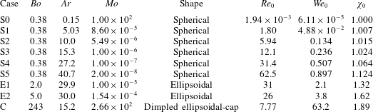
We considered nine different cases defined by the pair (
 $\mathit{Ar}$
,
 $\mathit{Bo}$
). A complete description of these cases and of the corresponding flow regimes is provided in table 1. They cover Reynolds numbers ranging from 0 to 60 and several shape regimes: spherical (cases ‘S’), ellipsoidal (cases ‘E’) and dimpled ellipsoidal cap (case ‘C’). The parameters for case C correspond to a single-bubble experiment of Bhaga & Weber (Reference Bhaga and Weber1981), which was later reproduced numerically by Hua, Stene & Lin (Reference Hua, Stene and Lin2008). The terminal Reynolds number and shape of the equivalent isolated bubble have therefore been determined directly from their data. For the other cases, the single-bubble terminal Reynolds number and aspect ratio have been estimated using the correlations for spherical and ellipsoidal bubbles recommended in the review of Loth (Reference Loth2008).
Simulated regimes:
 $\mathit{Bo}$
,
 $\mathit{Ar}$
and
 $\mathit{Mo}=\mathit{Bo}^{3}/\mathit{Ar}^{4}$
are input parameters (with
 $\unicode[STIX]{x1D70C}_{d}/\unicode[STIX]{x1D70C}_{c}=10^{-3}$
and
 $\unicode[STIX]{x1D707}_{d}/\unicode[STIX]{x1D707}_{c}=10^{-2}$
). The shapes,
 $\mathit{Re}_{0}$
,
 $\mathit{We}_{0}=\mathit{Bo}\mathit{Re}_{0}^{2}/\mathit{Ar}^{2}$
and
 $\unicode[STIX]{x1D712}_{0}$
of an isolated buoyancy-driven bubble at steady state are also given. Shapes are predicted by the diagram of Grace (Reference Grace1973). The values of
 $\mathit{Re}_{0}$
are estimated from the correlation of Mei, Klausner & Lawrence (Reference Mei, Klausner and Lawrence1994) for spherical bubbles (cases S0–S5) and from the correlation of Loth (Reference Loth2008) for ellipsoidal bubbles (cases E1 and E2); the experimental value measured by Bhaga & Weber (Reference Bhaga and Weber1981) is reported for case C. The aspect ratio
 $\unicode[STIX]{x1D712}_{0}$
is estimated from the correlation of Loth (Reference Loth2008) for all cases except case C, for which it is directly measured from visualizations of Hua et al. (Reference Hua, Stene and Lin2008).

2.3 Governing equations
In both phases the fluid motion is governed by the incompressible Navier–Stokes equations
 $$\begin{eqnarray}\displaystyle & \displaystyle \unicode[STIX]{x1D735}\boldsymbol{\cdot }\boldsymbol{u}_{n}=0, & \displaystyle\end{eqnarray}$$
 $$\begin{eqnarray}\displaystyle & \displaystyle \frac{\unicode[STIX]{x2202}\unicode[STIX]{x1D70C}_{n}\boldsymbol{u}_{n}}{\unicode[STIX]{x2202}t}+\unicode[STIX]{x1D735}\boldsymbol{\cdot }\unicode[STIX]{x1D70C}_{n}\boldsymbol{u}_{n}\boldsymbol{u}_{n}=\unicode[STIX]{x1D735}\boldsymbol{\cdot }\unicode[STIX]{x1D64F}_{n}+\boldsymbol{G}_{n}\quad \text{where }\unicode[STIX]{x1D64F}_{n}=-p_{n}\unicode[STIX]{x1D644}+\unicode[STIX]{x1D707}_{n}(\unicode[STIX]{x1D735}\boldsymbol{u}_{n}+\unicode[STIX]{x1D735}\boldsymbol{u}_{n}^{\text{T}}), & \displaystyle\end{eqnarray}$$
where
 $n=\{c,d\}$
is used here to denote either phase,
 $\boldsymbol{u}$
is the velocity field,
 $\unicode[STIX]{x1D64F}$
the stress tensor,
 $\unicode[STIX]{x1D644}$
denotes the identity tensor,
 $p$
the pressure field and
 $\boldsymbol{G}$
is the sum of external forces per unit volume, given by
 $\boldsymbol{G}_{n}=(\unicode[STIX]{x1D70C}_{n}-\langle \unicode[STIX]{x1D70C}\rangle )\boldsymbol{g}$
. The first term in this last expression,
 $\unicode[STIX]{x1D70C}_{n}\boldsymbol{g}$
, is the weight of a unit volume of fluid. Because the suspension we consider is infinite, i.e. not bounded by walls, an additional body force
 $-\langle \unicode[STIX]{x1D70C}\rangle \boldsymbol{g}$
, with
 $\langle \unicode[STIX]{x1D70C}\rangle$
the system average density, is required to prevent the entire system from accelerating in the downward vertical direction. (This body force is equivalent to the average hydrostatic pressure gradient that would be generated by the base of a flow container to balance the total gravitational force on the mixture.)
These equations are coupled through the appropriate boundary conditions at the interface. In the presence of viscous effects a no-slip condition is applied, which, combined with the absence of mass flux across the interface, leads to
 $$\begin{eqnarray}[\boldsymbol{u}]=\mathbf{0},\end{eqnarray}$$
where
 $[X]=X_{c}-X_{d}$
denotes the jump of a variable across the interface. Neglecting any variation of surface tension along the interface, the shear stress is continuous across it and the jump of normal stress is balanced by the curvature force per unit area:
 $$\begin{eqnarray}[\boldsymbol{n}\boldsymbol{\cdot }\unicode[STIX]{x1D64F}]=\unicode[STIX]{x1D6FE}\unicode[STIX]{x1D705}\boldsymbol{n},\end{eqnarray}$$
where
 $\boldsymbol{n}$
is the unit vector normal to the interface and directed outward from the bubbles and
 $\unicode[STIX]{x1D705}$
is the interface curvature defined by
 $\unicode[STIX]{x1D705}=\unicode[STIX]{x1D735}\boldsymbol{\cdot }\boldsymbol{n}$
(e.g. Tryggvason, Scardovelli & Zaleski (Reference Tryggvason, Scardovelli and Zaleski2011), appendix A.4).
This set of equations is solved numerically within a periodic unit cell using the methods described in the next section.
3 Numerical methods
A comprehensive description of our numerical approach is provided in § A.1. A brief overview of its salient features is given hereinafter.
Our approach relies on the one-fluid formulation of the governing equations. In this formulation, the different fluids are treated as a single phase with discontinuous density and viscosity, and surface tension is incorporated as a singular source term. This results in the standard continuum surface force model of Brackbill, Kothe & Zemach (Reference Brackbill, Kothe and Zemach1992). To circumvent numerical difficulties due to the introduction of discontinuous and singular functions, the interface is given a finite thickness proportional to the grid spacing. Surface tension is therefore treated as a volume force distributed over several mesh points and material properties vary continuously from one phase to the other.
The incompressible Navier–Stokes equations are integrated in their one-fluid form by a projection method (Chorin Reference Chorin1968), and the moving interface separating the two fluids is captured by a level-set method (Osher & Sethian Reference Osher and Sethian1988; Sussman, Smereka & Osher Reference Sussman, Smereka and Osher1994). The velocity field is then solution of the system of equations:
 $$\begin{eqnarray}\displaystyle & \displaystyle \frac{\unicode[STIX]{x2202}\unicode[STIX]{x1D70C}\boldsymbol{u}}{\unicode[STIX]{x2202}t}+\unicode[STIX]{x1D735}\boldsymbol{\cdot }\unicode[STIX]{x1D70C}\boldsymbol{u}\boldsymbol{u}=-\unicode[STIX]{x1D735}p+\unicode[STIX]{x1D735}\boldsymbol{\cdot }\unicode[STIX]{x1D707}(\unicode[STIX]{x1D735}\boldsymbol{u}+\unicode[STIX]{x1D735}\boldsymbol{u}^{\text{T}})+(\unicode[STIX]{x1D70C}-\langle \unicode[STIX]{x1D70C}\rangle )\boldsymbol{g}-\unicode[STIX]{x1D6FE}\unicode[STIX]{x1D705}\unicode[STIX]{x1D735}H_{\unicode[STIX]{x1D700}} & \displaystyle\end{eqnarray}$$
 $$\begin{eqnarray}\displaystyle & \displaystyle \unicode[STIX]{x1D735}\boldsymbol{\cdot }\boldsymbol{u}=0, & \displaystyle\end{eqnarray}$$
where the interface curvature is calculated from (e.g. Prosperetti & Tryggvason (Reference Prosperetti and Tryggvason2007), § 3.5)
 $$\begin{eqnarray}\unicode[STIX]{x1D705}=\unicode[STIX]{x1D735}\boldsymbol{\cdot }\left(\frac{\unicode[STIX]{x1D735}\unicode[STIX]{x1D713}}{|\unicode[STIX]{x1D735}\unicode[STIX]{x1D713}|}\right),\end{eqnarray}$$
the variable density and viscosity are given by
 $$\begin{eqnarray}\unicode[STIX]{x1D70C}=H_{\unicode[STIX]{x1D700}}\unicode[STIX]{x1D70C}_{c}+(1-H_{\unicode[STIX]{x1D700}})\unicode[STIX]{x1D70C}_{d},\quad \unicode[STIX]{x1D707}=H_{\unicode[STIX]{x1D700}}\unicode[STIX]{x1D707}_{c}+(1-H_{\unicode[STIX]{x1D700}})\unicode[STIX]{x1D707}_{d},\end{eqnarray}$$
and
 $H_{\unicode[STIX]{x1D700}}$
denotes the smoothed Heaviside function
 $$\begin{eqnarray}H_{\unicode[STIX]{x1D700}}(\unicode[STIX]{x1D713})=\left\{\begin{array}{@{}ll@{}}1\quad & \text{if }\unicode[STIX]{x1D713}>\unicode[STIX]{x1D700},\\ 0\quad & \text{if }\unicode[STIX]{x1D713}<-\unicode[STIX]{x1D700},\\ {\displaystyle \frac{1}{2}}\left[1+{\displaystyle \frac{\unicode[STIX]{x1D713}}{\unicode[STIX]{x1D700}}}+{\displaystyle \frac{1}{\unicode[STIX]{x03C0}}}\sin \left({\displaystyle \frac{\unicode[STIX]{x03C0}\unicode[STIX]{x1D713}}{\unicode[STIX]{x1D700}}}\right)\right]\quad & \text{if }|\unicode[STIX]{x1D713}|\leqslant \unicode[STIX]{x1D700},\end{array}\right.\end{eqnarray}$$
where
 $\unicode[STIX]{x1D700}$
is half the interface thickness (
 $\unicode[STIX]{x1D700}=1.5\unicode[STIX]{x0394}x$
, with
 $\unicode[STIX]{x0394}x$
the grid spacing).
 $\unicode[STIX]{x1D713}$
denotes the level-set function, positive in the continuous phase and negative in the disperse one. It is the solution of the following advection equation, in which the zeroth-order approximation of the additional source term proposed by Sabelnikov, Ovsyannikov & Gorokhovski (Reference Sabelnikov, Ovsyannikov and Gorokhovski2014) is embedded:
 $$\begin{eqnarray}\frac{\unicode[STIX]{x2202}\unicode[STIX]{x1D713}}{\unicode[STIX]{x2202}t}+\boldsymbol{u}\boldsymbol{\cdot }\unicode[STIX]{x1D735}\unicode[STIX]{x1D713}=A(\boldsymbol{u},\unicode[STIX]{x1D713})\unicode[STIX]{x1D713},\quad \text{with }A(\boldsymbol{u},\unicode[STIX]{x1D713})=\unicode[STIX]{x1D735}_{i}\unicode[STIX]{x1D713}\unicode[STIX]{x1D735}_{i}u_{j}\unicode[STIX]{x1D735}_{j}\unicode[STIX]{x1D713}\end{eqnarray}$$
(
 $A(\boldsymbol{u},\unicode[STIX]{x1D713})$
is the local zeroth-order approximation of the source term in the region close to the interface). The level-set function is reinitialized as a signed distance function at each time step using the procedure devised by Russo & Smereka (Reference Russo and Smereka2000). These modifications yield better numerical efficiency and accuracy compared to the original level-set method.
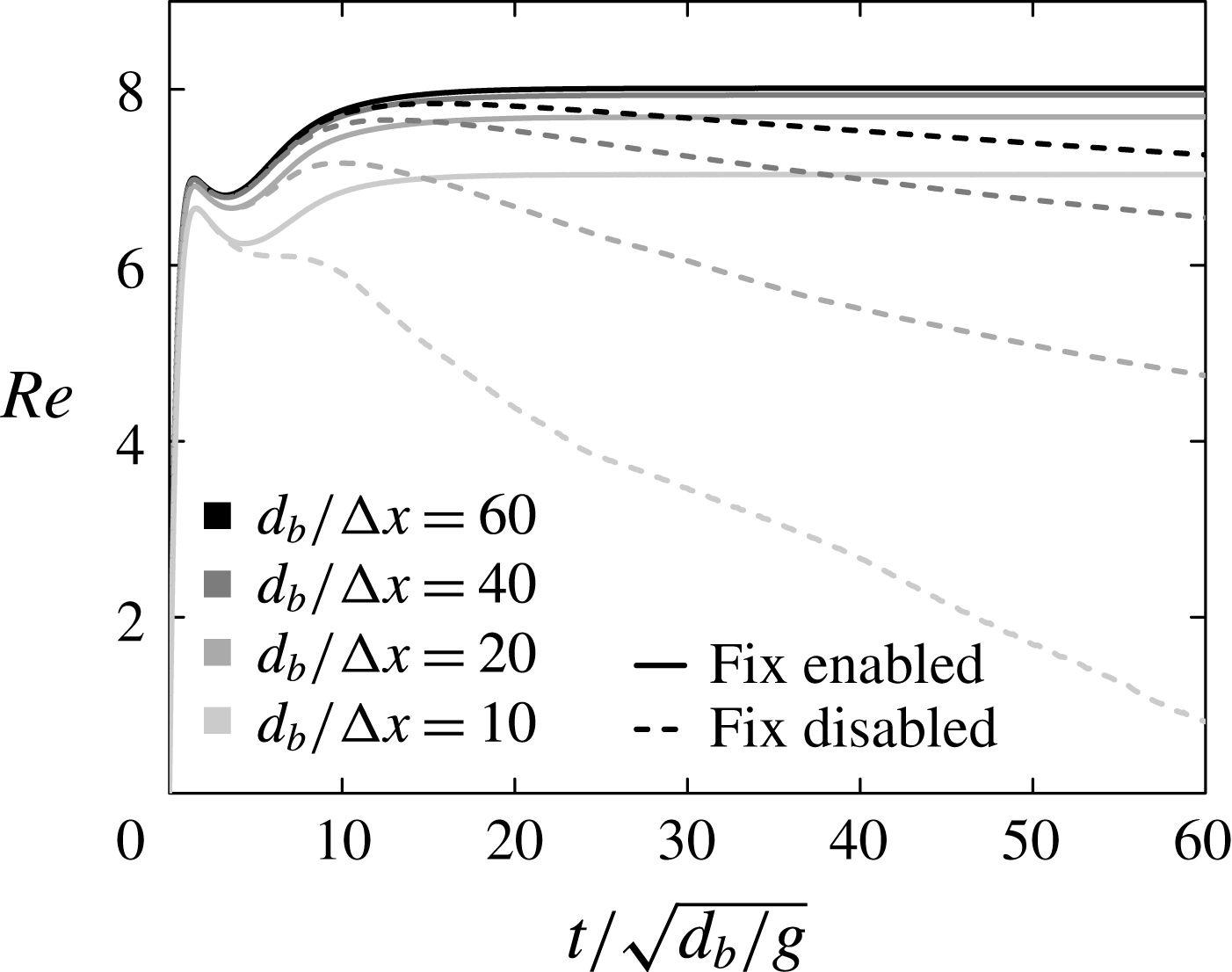
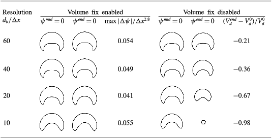
The major drawback of basic level-set methods is their poor ability to conserve the mass (volume) of each phase. When using high-order schemes and sufficient resolution, the volume change between two successive time steps is often negligible. It is, however, not exactly zero, and may even become substantial when accumulated over very long integration times. For this reason, we enforce volume conservation using the correction proposed by Sussman & Uto (Reference Sussman and Uto1998) (also used by e.g. Spelt (Reference Spelt2006)): at the end of each time step, the iso-contours of the level-set function are slightly shifted such that the volume of each phase is conserved exactly. We demonstrate in § A.2 that the loss of accuracy induced by this correction is negligible compared to the overall numerical error made in the interfacial region, and has therefore no adverse effect on the flow dynamics.
Our time integration algorithm is based on third-order and second-order total-variation-diminishing (TVD) Runge–Kutta schemes for the level-set advection and reinitialization equations, respectively, and on a mixed Crank–Nicolson/third-order Adams–Bashforth scheme for the Navier–Stokes equations. The spatial discretization is carried out using a standard finite-difference/finite-volume discretization on a uniform Cartesian staggered grid: fifth-order weighted-essentially-nonoscillatory (WENO) schemes are used for advection terms and second-order centred schemes are used otherwise. Periodic boundary conditions are imposed at the bounds of the computational domain.
A standard benchmark test for the simulation of disperse flows consists in comparing the terminal velocity and shape of an isolated bubble to those obtained experimentally in various regimes. We do not simulate here the rise of a single bubble in an unbounded fluid but of an array of bubbles. A tempting idea to approach this ideal situation would be to introduce a single bubble in a very large unit cell, so that the influence of periodicity could be neglected. We will see in § 4 that even at very low volume fractions (very large domains, in the limit of what is computationally feasible), the bubbles’ rise velocity and shape are still significantly affected by their interactions, making such a comparison to experiments irrelevant. The code has therefore been validated against available solutions for regular (
 $N_{b}=1$
) and free (
 $N_{b}>1$
) arrays of rising bubbles.
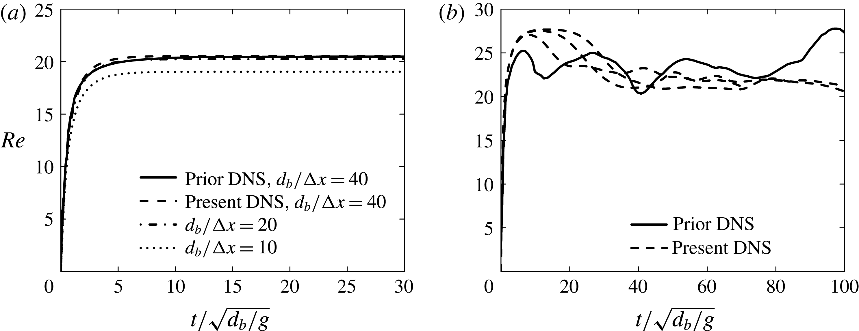
Time evolution of the drift velocity of arrays of deformable bubbles rising at moderate Reynolds numbers (case E1). Solid line: prior DNS of Esmaeeli & Tryggvason (Reference Esmaeeli and Tryggvason1999). Non-solid lines: present DNS. (a) Ordered array (
 $N_{b}=1$
,
 $\unicode[STIX]{x1D719}=13$
%,
 $\unicode[STIX]{x1D70C}_{d}/\unicode[STIX]{x1D70C}_{c}=\unicode[STIX]{x1D707}_{d}/\unicode[STIX]{x1D707}_{c}=0.1$
), different resolutions (
 $d_{b}$
is the bubble volume-equivalent diameter,
 $\unicode[STIX]{x0394}x$
the grid spacing). (b) Free array (
 $N_{b}=8$
,
 $\unicode[STIX]{x1D719}=6.5$
%,
 $\unicode[STIX]{x1D70C}_{d}/\unicode[STIX]{x1D70C}_{c}=\unicode[STIX]{x1D707}_{d}/\unicode[STIX]{x1D707}_{c}=0.05$
), with three realizations of the flow.

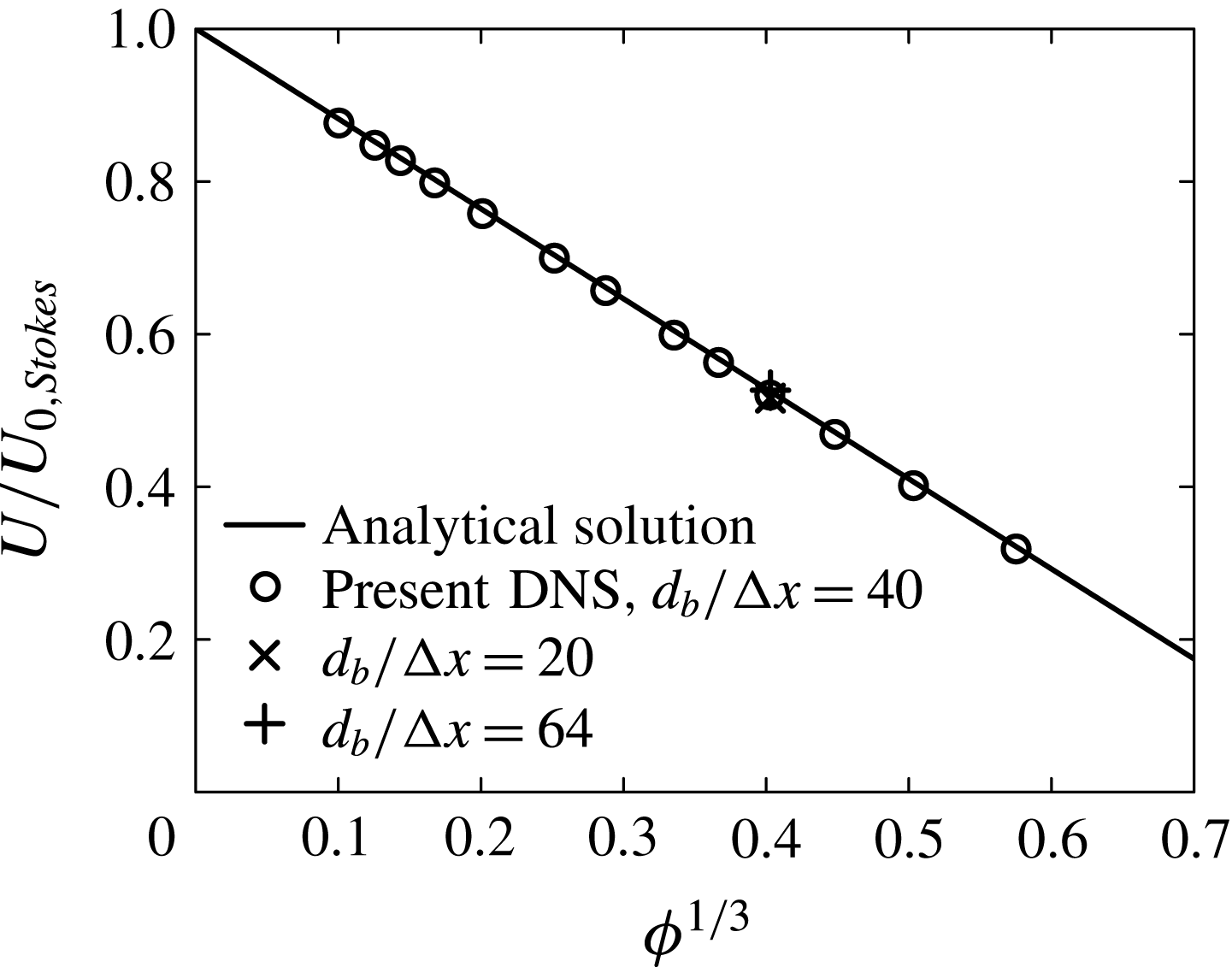
We reproduced the numerical simulations of Esmaeeli & Tryggvason (Reference Esmaeeli and Tryggvason1999) who considered arrays of deformable bubbles rising at moderate Reynolds number (case E1). As shown in figure 1, the transient rise of both regular and free arrays of bubbles is reproduced accurately by our code. We also compared our simulations with the theory of Sangani (Reference Sangani1987) for cubic arrays of spherical bubbles in the creeping flow limit (case S0). The evolution of the steady drift velocity with volume fraction is shown in figure 2. Excellent agreement between the numerical and analytical solutions has been obtained. The effect of resolution is also shown in the same figures. Additional benchmark and sensitivity tests can be found in § A.2. Further comparison against prior work is included where prior work is available in subsequent sections.
Grid convergence tests have been carried out systematically for each of the cases reported in table 1 in an ordered array configuration and for one value of the volume fraction. A resolution of 20 grid cells per bubble diameter was found to be sufficient for all regimes except for case S5, which requires a resolution of 30 grid cells per diameter because of the higher Reynolds numbers associated with this regime, and for case C, for which a resolution of 60 grid cells per diameter was needed for capturing the thin skirts of the bubbles. With these resolutions, the error in the steady rise velocity due to the grid spacing is not larger than 2 % in case C and 1 % in the other cases. For a given case, the same resolution is used for all volume fractions and for both ordered and free arrays. The choice of the time step is constrained by the condition of numerical stability and the error due to the time discretization is smaller than that due to the spatial one.
Steady drift velocity of an ordered array of spherical bubbles normalized by that of an isolated bubble in the Stokes flow regime (case S0) as a function of volume fraction, compared with the analytical solution of Sangani (Reference Sangani1987). The effect of resolution is shown for
 $\unicode[STIX]{x1D719}^{1/3}=0.4$
(
 $d_{b}$
is the bubble volume-equivalent diameter,
 $\unicode[STIX]{x0394}x$
the grid spacing).

4 Ordered arrays
We examine in this section the dynamics of cubic arrays of deformable bubbles (‘ordered arrays’) in the presence of liquid inertia. The main objective here is to connect DNS results, theoretical analysis for dilute systems and prior work on bubble pairs.
Specifically, the effect of volume fraction on the rise velocity and shape of deformable bubbles in a simple cubic array is revisited here. Direct numerical simulations have been performed for the nine sets of flow conditions summarized in table 1. For each of these cases, the volume fraction
 $\unicode[STIX]{x1D719}=\unicode[STIX]{x03C0}/6(d_{b}/h)^{3}$
(where
 $h$
is the linear size of the unit cell of the array) was varied from 0.1 % to 30 % by changing the size of the computational domain (i.e. the lattice spacing) while keeping the bubble size constant.
Initially, both fluids were at rest, the bubbles were spherical and gravity was switched on at time zero. After a transient regime, various forms of bubble motion could be observed: steady vertical rise, steady oblique rise or unsteady oblique rise. The steady vertical rise is first examined in § 4.1. Other types of motions are then discussed in § 4.2.
Simulations were run until the bubble drift velocity became either constant or statistically stationary. This steady state is independent of the initial oblateness of the bubbles, and is reached when the velocity disturbances induced by the bubbles’ motion have diffused in all directions throughout the liquid, i.e. in a time of order
 $O(h^{2}\unicode[STIX]{x1D70C}_{c}/\unicode[STIX]{x1D707}_{c})$
. As a consequence, from a numerical point of view, the investigation of small volume fractions (large domain sizes) is limited both by the needed number of grid points (
 ${\sim}h^{3}$
) and by the computation time (
 ${\sim}h^{2}$
).
4.1 Steady vertical rise of bubbles
The cubic lattice of bubbles is not only convenient from a computational point of view, it is also attractive from a theoretical standpoint since the solution only needs to be determined in a unit cell. When the bubbles rise steadily along straight paths parallel to an axis of the periodic array (as is the case in most of the cases presented here since gravity is oriented along a lattice axis), the symmetries of the problem greatly simplify the analysis. We determine in this context an analytical expression accounting for the first effect of inertial interactions in cubic arrays of spherical bubbles (at small Reynolds numbers). Outside this narrow range of validity, the influence of the volume fraction on the steady rise velocity and shape of deformable bubbles will be determined from our numerical simulations.
4.1.1 Spherical bubbles at low to moderate Reynolds number
The correction to the drift velocity due to finite volume fraction in the Stokes flow regime has been determined by Sangani (Reference Sangani1987) for cubic arrays of spherical fluid particles (bubbles or drops). The first term arises from a point-force approximation of the particles and reads, for a simple cubic array,
 $$\begin{eqnarray}\frac{U}{U_{0,Stokes}}-1=-1.1734\unicode[STIX]{x1D707}^{\ast }\unicode[STIX]{x1D719}^{1/3}+O(\unicode[STIX]{x1D719}),\end{eqnarray}$$
where
 $U_{0,Stokes}$
is the terminal velocity of a spherical fluid particle translating through an unbounded ambient fluid in Stokes flow conditions (Hadamard Reference Hadamard1911; Rybczynski Reference Rybczynski1911):
 $$\begin{eqnarray}U_{0,Stokes}=\frac{1}{12}\frac{|\unicode[STIX]{x1D70C}_{c}-\unicode[STIX]{x1D70C}_{d}|gd_{b}^{2}}{\unicode[STIX]{x1D707}^{\ast }\unicode[STIX]{x1D707}_{c}},\quad \text{with }\unicode[STIX]{x1D707}^{\ast }=\frac{\unicode[STIX]{x1D707}_{c}+3\unicode[STIX]{x1D707}_{d}/2}{\unicode[STIX]{x1D707}_{c}+\unicode[STIX]{x1D707}_{d}}.\end{eqnarray}$$
The case of a rigid sphere (
 $\unicode[STIX]{x1D707}_{d}/\unicode[STIX]{x1D707}_{c}\rightarrow \infty$
) is recovered as
 $\unicode[STIX]{x1D707}^{\ast }\rightarrow 3/2$
, whereas the case of a clean bubble (
 $\unicode[STIX]{x1D707}_{d}/\unicode[STIX]{x1D707}_{c}\rightarrow 0$
) corresponds to the limit
 $\unicode[STIX]{x1D707}^{\ast }\rightarrow 1$
. Numerical simulations have been carried out for spherical bubbles rising at very small Reynolds numbers (case S0,
 $\mathit{Re}_{0}=1.94\times 10^{-3}$
), and excellent agreement with the theory has been obtained over a wide range of volume fractions, as shown in figure 2. Note that the relation between
 $U$
and
 $\unicode[STIX]{x1D719}^{1/3}$
seems linear even at high volume fraction: indeed, even though the analytical solution of Sangani (Reference Sangani1987) includes
 $O(\unicode[STIX]{x1D719})$
and
 $O(\unicode[STIX]{x1D719}^{2})$
terms, for clean bubbles the
 $O(\unicode[STIX]{x1D719})$
correction is zero and the
 $O(\unicode[STIX]{x1D719}^{2})$
correction is negligible compared to the
 $O(\unicode[STIX]{x1D719}^{1/3})$
term (whereas these corrections are substantial for solid particles).
For small but non-zero Reynolds numbers, the Stokes equations are still valid near and inside the fluid particles, but should be replaced by the Oseen equations farther away since inertial effects become comparable to viscous ones at distances from the particle of order
 $O(d_{b}/\mathit{Re})$
. The first correction to the drag force arising from inertial effects has been determined by Hill, Koch & Ladd (Reference Hill, Koch and Ladd2001) for a cubic array of solid spheres. The extension of their result to bubbles and drops is straightforward and is provided in appendix B. We show there that the correction to the bubble drift velocity due to liquid inertia and hydrodynamic interactions can be approximated at any
 $\unicode[STIX]{x1D719}\ll 1$
by
 $$\begin{eqnarray}\frac{U}{U_{0,Stokes}}-1\approx -\frac{1}{8}\unicode[STIX]{x1D707}^{\ast }\mathit{Re}-1.1734\unicode[STIX]{x1D707}^{\ast }\unicode[STIX]{x1D719}^{1/3}+\frac{25}{8}\unicode[STIX]{x1D707}^{\ast }\frac{\mathit{Re}\unicode[STIX]{x1D719}^{1/3}}{\mathit{Re}+25\unicode[STIX]{x1D719}^{1/3}}.\end{eqnarray}$$
The first term accounts for the effect of liquid inertia on an isolated bubble, the second term results from Stokes interactions and the last term captures the effect of inertial interactions. The significance of each of these terms as a function of volume fraction can be understood as follows.
At zero volume fraction, the drag exerted on a single bubble normalized by the Stokes drag increases linearly with the Reynolds number (Brenner & Cox Reference Brenner and Cox1963). This results in the negative correction to the drift velocity
 $$\begin{eqnarray}\frac{U_{0}}{U_{0,Stokes}}-1=-\frac{1}{8}\unicode[STIX]{x1D707}^{\ast }\mathit{Re},\end{eqnarray}$$
where
 $U_{0}$
is the terminal velocity of the isolated bubble. At small volume fraction, inertial interactions result in a positive
 $O(\unicode[STIX]{x1D719}^{1/3})$
correction which overwhelms the negative
 $O(\unicode[STIX]{x1D719}^{1/3})$
Stokes flow correction
 $$\begin{eqnarray}\frac{U-U_{0}}{U_{0,Stokes}}\approx -1.1734\unicode[STIX]{x1D707}^{\ast }\unicode[STIX]{x1D719}^{1/3}+\frac{25}{8}\unicode[STIX]{x1D707}^{\ast }\unicode[STIX]{x1D719}^{1/3}\approx 2.0\unicode[STIX]{x1D707}^{\ast }\unicode[STIX]{x1D719}^{1/3}\quad \text{when }\unicode[STIX]{x1D719}^{1/3}\ll \mathit{Re},\end{eqnarray}$$
so the net result is a drift velocity that increases with
 $\unicode[STIX]{x1D719}^{1/3}$
. At large volume fraction (with respect to the Reynolds number), the drift velocity correction due to hydrodynamic interactions reads
 $$\begin{eqnarray}\frac{U-U_{0}}{U_{0,Stokes}}=-1.1734\unicode[STIX]{x1D707}^{\ast }\unicode[STIX]{x1D719}^{1/3}+\frac{1}{8}\unicode[STIX]{x1D707}^{\ast }\mathit{Re}\left(1-\frac{\mathit{Re}}{25\unicode[STIX]{x1D719}^{1/3}}\right)\quad \text{when }\mathit{Re}\ll \unicode[STIX]{x1D719}^{1/3}\ll 1.\end{eqnarray}$$
The
 $O(\mathit{Re})$
contribution from inertia is negligible compared to the Stokes
 $O(\unicode[STIX]{x1D719}^{1/3})$
correction: the drift velocity therefore overall decreases linearly with
 $\unicode[STIX]{x1D719}^{1/3}$
, as for creeping flows.
The drift velocity
 $U$
can be computed, for any
 $\unicode[STIX]{x1D719}\ll 1$
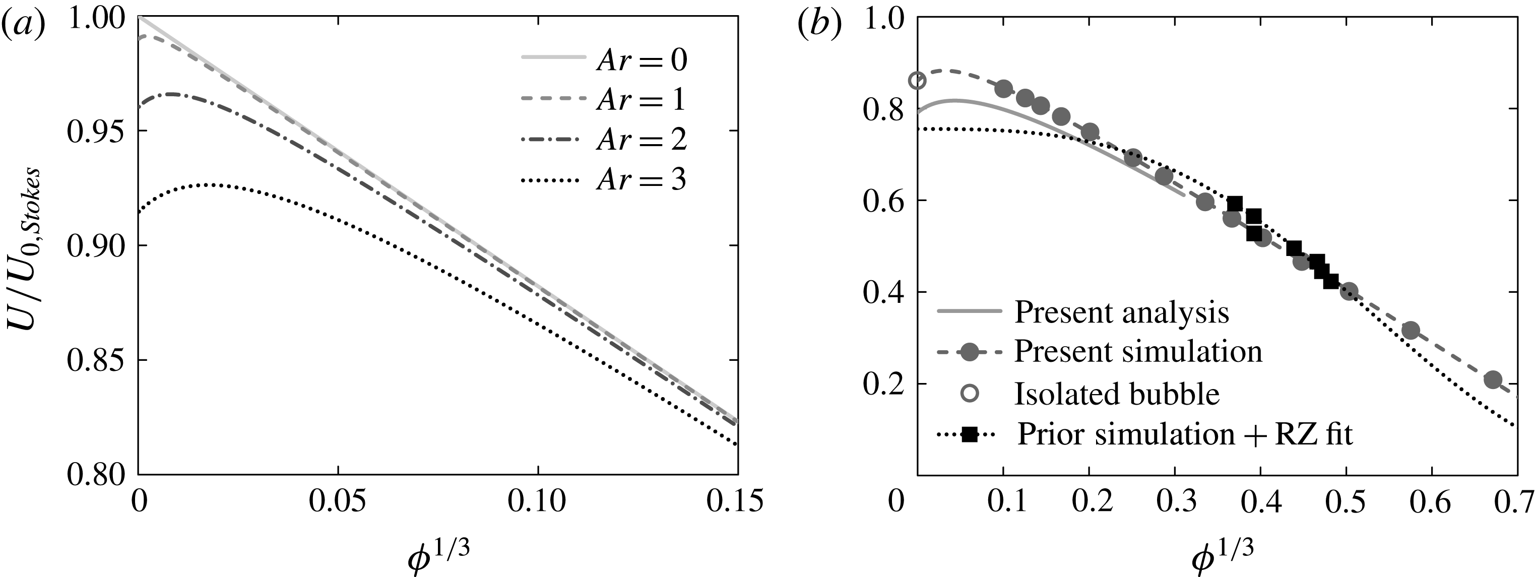
, by finding the positive root of (4.3) (quadratic in
 $U$
). The solution for various Archimedes numbers is shown in figure 3(a). Note that higher Archimedes number corresponds to higher isolated-bubble Reynolds number: it can be shown from (2.1), (2.4), (4.2) and (4.4) that in this regime
 $$\begin{eqnarray}\mathit{Re}_{0}=\frac{1}{12}\frac{\mathit{Ar}^{2}}{\unicode[STIX]{x1D707}^{\ast }}\left(1+\frac{\mathit{Ar}^{2}}{96}\right)^{-1}.\end{eqnarray}$$
The non-monotonicity of the function
 $U(\unicode[STIX]{x1D719})/U_{0,Stokes}$
at finite Archimedes number contrasts with the case of Stokes flow, for which this function is strictly decreasing. This behaviour results from the competition between ‘cooperative’ long-range inertial interactions, which increase the drift velocity and ‘hindering’ viscous interactions which reduce it. At small volume fraction, inertial effects dominate, whereas at large volume fraction the liquid is more confined, inertial forces therefore cannot prevail over viscous ones and a Stokes flow behaviour is recovered.
Steady drift velocity of an ordered array of spherical bubbles, normalized by the terminal velocity of an isolated bubble in Stokes flow conditions, as a function of volume fraction for small Archimedes numbers. (a) The effect of small but finite
 $\mathit{Ar}$
, from Oseen flow analysis. (b) Comparison of analytical and numerical solutions for
 $\mathit{Ar}=5.03$
(case S1). Analytical solutions are obtained from (4.3). Symbols in (b): ——, analysis; ●, DNS; ○, isolated bubble, estimated from Mei et al. (Reference Mei, Klausner and Lawrence1994); – – – –, numerical fit of the form of (4.8) matching DNS and isolated-bubble data; and ▪ and
 $\cdots \cdots$
, numerical data and fit by a Richardson–Zaki relation from Sankaranarayanan et al. (Reference Sankaranarayanan, Shan, Kevrekidis and Sundaresan2002).

The Oseen approximation is limited to
 $\mathit{Re}<1$
, which for an isolated clean bubble approximately corresponds to
 $\mathit{Ar}<3.5$
. For
 $\mathit{Ar}=3$
, the maximum of
 $U/U_{0,Stokes}$
is obtained for
 $\unicode[STIX]{x1D719}=6\times 10^{-6}$
. Direct numerical simulation of such a small volume fraction is prohibitively expensive, so our analysis cannot be confirmed by numerical experiments in its expected range of validity. Nevertheless, a comparison between the solution obtained from (4.3) and DNS for
 $\mathit{Ar}=5.03$
is shown in figure 3(b), together with the numerical data obtained by Sankaranarayanan et al. (Reference Sankaranarayanan, Shan, Kevrekidis and Sundaresan2002) for the identical flow regime using the lattice Boltzmann method. In their study, they found that the effect of volume fraction could be captured by a Richardson–Zaki type of (empirical) correlation
 $\mathit{Re}=1.58(1-\unicode[STIX]{x1D719})^{4.72}$
. Although their data are well fitted by this relation over the narrow range of volume fractions they investigated (
 $0.05<\unicode[STIX]{x1D719}<0.12$
), our DNS results show that this expression cannot be used to extrapolate the effect of volume fraction outside this range. In addition, their correlation gives a drift velocity at
 $\unicode[STIX]{x1D719}=0$
that differs from the terminal velocity of an isolated bubble by more than 10 %. In contrast, the functional dependency of the drift velocity on volume fraction given by our analysis is in very good agreement with numerical simulations; the modest difference at small volume fractions arises from the limitation of Oseen theory to Reynolds numbers less than unity: for an isolated bubble rising in still liquid, the Oseen flow solution yields
 $\mathit{Re}_{0}=1.66$
whereas the empirical correlation of Mei et al. (Reference Mei, Klausner and Lawrence1994) gives
 $\mathit{Re}_{0}=1.80$
.
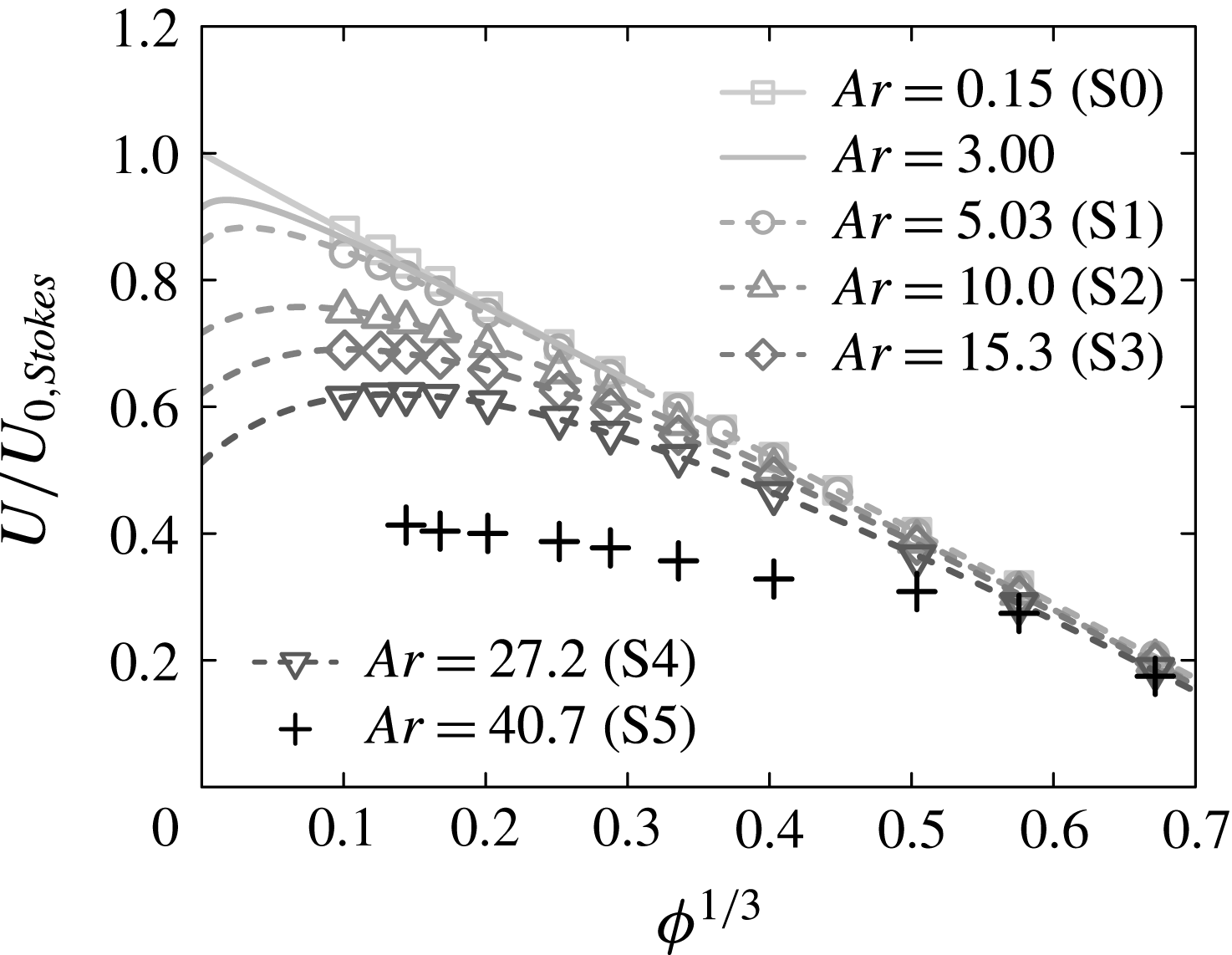
We now turn to ordered arrays of spherical bubbles rising at moderate Reynolds numbers. The bubble drift velocity has been determined for Archimedes numbers ranging from 0 to 40 (cases S0–S5). The numerical results for
 $U(\unicode[STIX]{x1D719})/U_{0,Stokes}$
are shown in figure 4 (symbols) together with those of our analysis for small Archimedes numbers (solid lines). It is remarkable that the evolution of the drift velocity with volume fraction for Archimedes numbers up to approximately 30 is consistent with the Oseen flow analysis carried out for Archimedes numbers that are, at best,
 $O(1)$
. In particular, for
 $\mathit{Ar}=27.2$
(case S4), the predicted increase of the drift velocity at low volume fraction is confirmed numerically. For Archimedes numbers greater than 30 (case S5), the drift velocity of a cubic array of spherical bubbles does not necessarily remain parallel to gravity; we postpone discussion of this to § 4.2.
Steady drift velocity of an ordered array of spherical bubbles, normalized by the terminal velocity of an isolated bubble in Stokes flow conditions, as a function of volume fraction for a large range of Archimedes numbers. Symbols, DNS; ——, analytical Oseen flow solutions obtained from (4.3) for small
 $\mathit{Ar}$
; – – – –, numerical fits of the form of (4.8) matching DNS and isolated-bubble data for larger
 $\mathit{Ar}$
. In case S5, for which the bubbles’ motion is not steady and/or not parallel to gravity, the crosses are time-averaged vertical drift velocities.

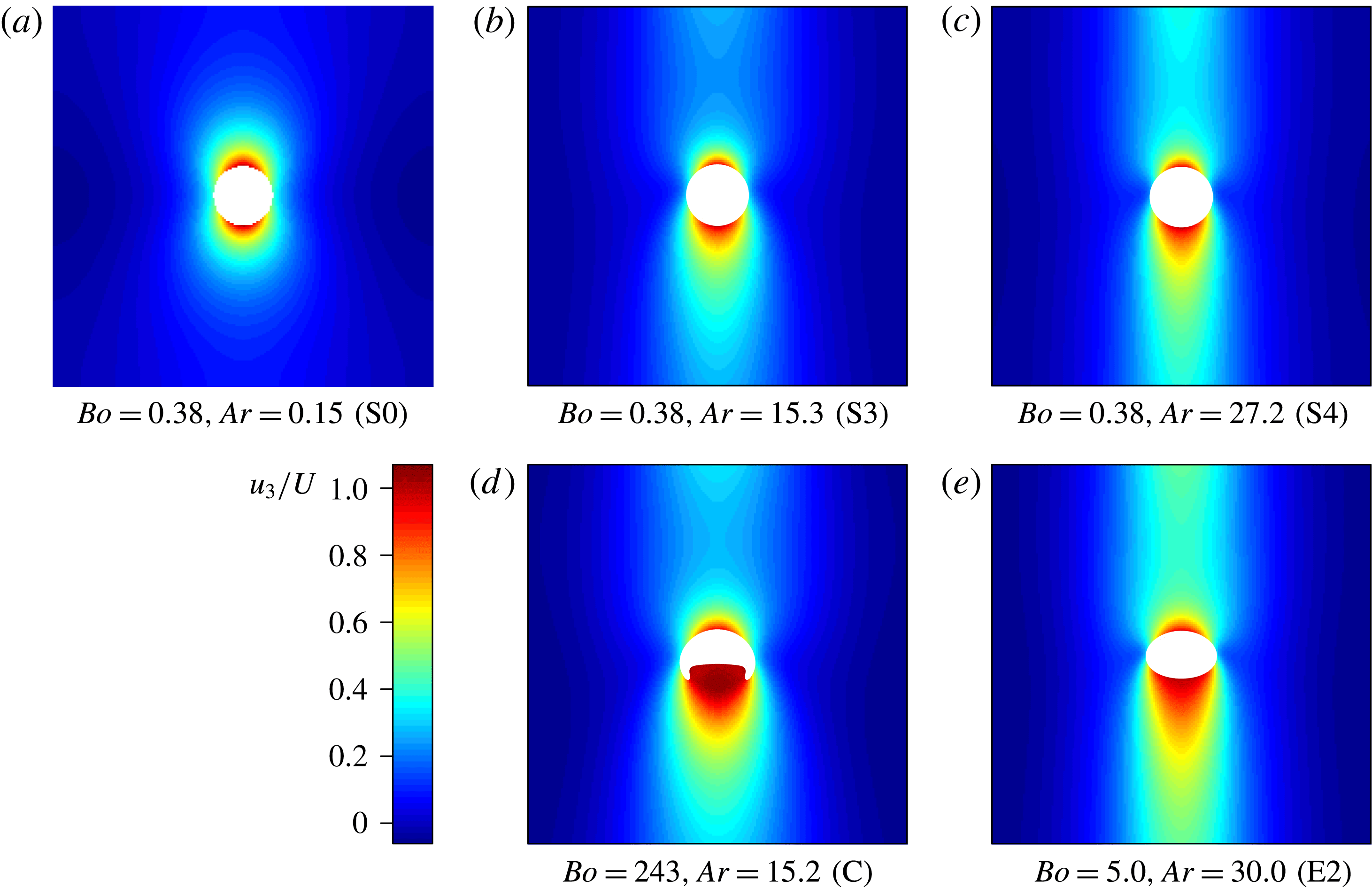
Figure 5 shows the vertical component of the liquid velocity in a vertical symmetry plane passing through the centre of a bubble at
 $\unicode[STIX]{x1D719}=0.2$
%. The first row corresponds to spherical bubbles (
 $\mathit{Bo}=0.38$
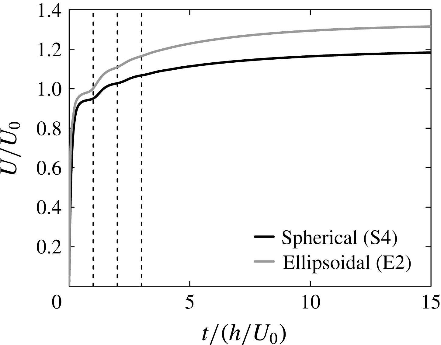
) with increasing Archimedes numbers from left to right. It reveals that the region of liquid dragged up by each bubble extends quite far downstream. Since the bubble motion is parallel to a primary axis of the array, each bubble benefits from this upwards motion by its ‘upstairs’ neighbour(s). This effect is stronger at larger Archimedes numbers, corresponding to higher Reynolds numbers and for which the wakes of the bubbles therefore extend further downstream. Cooperative rise is thus due to the strong wake interactions between vertically aligned bubbles. Wake interactions are also visible in the transient evolution of the drift velocity shown in figure 6. This quantity first levels off after an initial transient, then the bubbles experience a significant acceleration at
 $t=O(h/U_{0})$
that is as they enter into the wake of their first preceding neighbour. At the smallest volume fraction considered, the time scales separation and the wakes strengths are sufficient to distinguish the same phenomenon at
 $t\approx 2h/U_{0}$
: the bubbles’ rise is then influenced by the wake of their second preceding neighbour, they accelerate again, and so on until convergence.
Vertical component of the liquid velocity normalized by the bubble drift velocity in a vertical symmetry plane passing through the centre of a bubble in an ordered array configuration at
 $\unicode[STIX]{x1D719}=0.2$
%. Gravity is pointing downward (
 $\boldsymbol{g}=-g\boldsymbol{e}_{3}$
). Increasing Archimedes numbers from left to right, and increasing Bond numbers from top to bottom.

Time signal of the normalized drift velocity of an ordered array of bubbles at small volume fraction (
 $\unicode[STIX]{x1D719}=0.1$
%). The dashed vertical lines denote
 $t=nh/U_{0}$
, the characteristic times at which the bubbles enter into the wake of their
 $n\text{th}$
preceding neighbour. For clarity only short times are shown (the steady state is reached for
 $t\approx 50h/U_{0}$
).

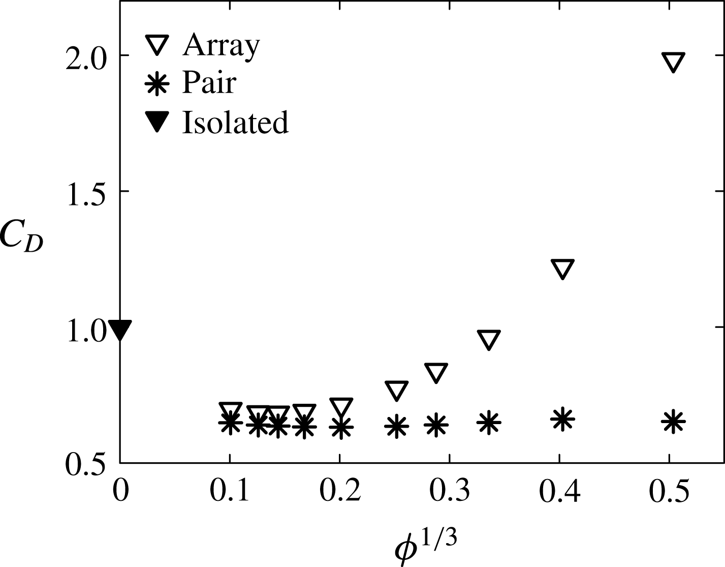
To complete this analysis we now evaluate how a simple prediction based on pair interaction compares with our results. We estimate for this the drag coefficient of the trailing bubble of a vertically aligned pair separated by a distance
 $h$
(our lattice spacing) and translating with a velocity
 $U$
identical to that of the array of bubbles at the corresponding volume fraction
 $\unicode[STIX]{x1D719}=\unicode[STIX]{x03C0}/6(d_{b}/h)^{3}$
using the model of Hallez & Legendre (Reference Hallez and Legendre2011) (equation (6.7) therein). Their expression, which accounts for potential and wake interactions, has been established for
 $\mathit{Re}\geqslant 20$
, so we show in figure 7 the results obtained for case S4 and
 $\unicode[STIX]{x1D719}^{1/3}<0.55$
, where this condition is met. At very small volume fraction (
 $\unicode[STIX]{x1D719}^{1/3}\lesssim 0.13$
), the drag acting on a bubble of the array is comparable to that exerted on the trailing bubble of a pair rising in line, as expected since in dilute conditions, wake interaction between vertically aligned neighbours dominates. At elevated volume fraction, the dimensionless distance between vertically aligned bubbles
 $h/d_{b}$
is smaller, but the drag is no longer governed primarily by such pair interactions, as the departure from the pair interaction results is seen to be substantial in figure 7.
Drag coefficient as a function of volume fraction for case S4. ▿, ordered array; *, trailing bubble of a vertically aligned pair within the same conditions (Reynolds number, separation distance), from Hallez & Legendre (Reference Hallez and Legendre2011); ▾, isolated bubble, estimated from Mei et al. (Reference Mei, Klausner and Lawrence1994).

4.1.2 Deformed bubbles at moderate Reynolds numbers
We now examine the effect of the Bond number on bubble deformation and on hydrodynamic interactions. The effect of volume fraction on
 $U/U_{0}$
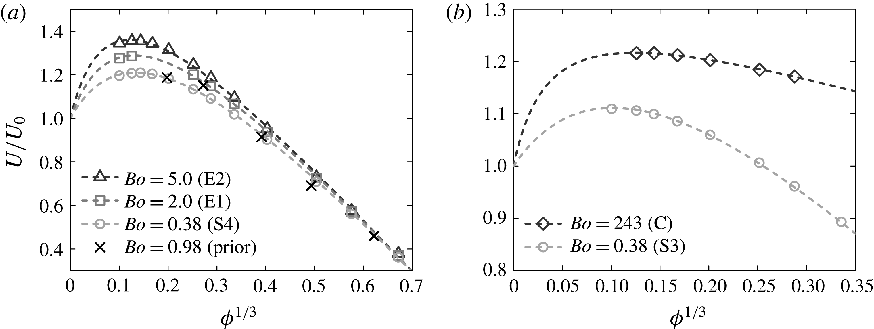
is first shown, for different values of the Bond number and comparable Archimedes numbers, in figure 8(a) (
 $\mathit{Ar}\approx 30$
) and figure 8(b) (
 $\mathit{Ar}\approx 15$
). The data points that are apparently missing at some intermediate volume fractions for case E1 actually correspond to bubbles that do not rise steadily and vertically (discussion of these is postponed to § 4.2 and figure 15
a), and only small volume fractions are shown for case C because bubbles cannot exist at higher
 $\unicode[STIX]{x1D719}$
(instead, unsteady elongated bodies of gas are obtained). We have also included in figure 8(a) the numerical data obtained by Bunner & Tryggvason (Reference Bunner and Tryggvason2002a
), who noticed that normalized drift velocities could be larger than unity at low volume fraction (black crosses). In their study, they estimated
 $\mathit{Re}_{0}=36$
by interpolating the data of Ryskin & Leal (Reference Ryskin and Leal1984). Using the correlation of Loth (Reference Loth2008), as we did for our own sets of parameters, we obtained
 $\mathit{Re}_{0}=33$
. For consistency we kept this value for replotting their data. Their results follow approximately the same trend as ours, although their normalized drift velocities are slightly lower. This is probably because the effect of the gas viscosity is assumed to be zero when estimating
 $\mathit{Re}_{0}$
, a hypothesis better approached by our DNS than by that from Bunner & Tryggvason (Reference Bunner and Tryggvason2002a
), who used a gas viscosity twice as large.
Normalized steady drift velocity of an ordered array of deformable bubbles as a function of volume fraction for various Bond numbers. (a)
 $\mathit{Ar}\approx 30$
: spherical and ellipsoidal bubbles. (b)
 $\mathit{Ar}\approx 15$
: spherical and dimpled ellipsoidal-cap bubbles. Open symbols: present DNS. Black crosses: prior DNS of Bunner & Tryggvason (Reference Bunner and Tryggvason2002a
) (
 $\mathit{Ar}=29.7$
,
 $\mathit{Bo}=0.98$
,
 $\unicode[STIX]{x1D70C}_{d}/\unicode[STIX]{x1D70C}_{c}=\unicode[STIX]{x1D707}_{d}/\unicode[STIX]{x1D707}_{c}=0.02$
). Dashed lines: numerical fits of the form of (4.8) matching DNS and isolated-bubble data.

The shape of
 $U(\unicode[STIX]{x1D719})/U_{0}$
, specifically its non-monotonicity, is similar to that obtained for spherical bubbles, but the faster rise at small volume fraction is more pronounced at higher Bond numbers. The origin of this behaviour becomes clear if one examines the effect of the Bond number on bubble wakes in figure 5, in which the vertical component of the liquid velocity is represented in a vertical symmetry plane at small volume fraction (
 $\unicode[STIX]{x1D719}=0.2$
%). Each column corresponds to comparable Archimedes numbers (
 $\mathit{Ar}\approx 15$
and
 $30$
for the second and third columns, respectively) with increasing Bond numbers from top to bottom. As the Bond number increases, the bubbles flatten (as discussed below) and their drag coefficient increases (for a given
 $\mathit{Re}$
) as a result of the increase of their frontal area (e.g. Loth Reference Loth2008). This induces greater upward liquid velocities in their wakes and therefore stronger cooperative interactions between in-line objects. The transient evolution of the drift velocity is shown in figure 6. It is similar to that of spherical bubbles, with accelerations at time intervals
 $O(h/U_{0})$
but a slightly different initial transient in which the time dependence of acceleration is non-monotonic, a feature related to the bubble deformation from a sphere to an ellipsoid.
These results can be directly compared with those of Sankaranarayanan et al. (Reference Sankaranarayanan, Shan, Kevrekidis and Sundaresan2002), who found that the evolution of the drift velocity with the volume fraction follows a Richardson–Zaki relation
 $\mathit{Re}=\mathit{Re}_{0}(1-\unicode[STIX]{x1D719})^{n}$
(Richardson & Zaki Reference Richardson and Zaki1954), where
 $n$
is given by an empirical closure relation in terms of
 $\mathit{Re}_{0}\mathit{Bo}^{1/4}/\mathit{Ar}$
(in the present notation). The trends predicted by this relation strongly disagree with our numerical results, and are therefore not shown. Once again, it appears that this power law dependency on volume fraction may be used to obtain a coarse estimate of the drift velocity at high volume fraction, but does not capture the complex influence of hydrodynamic interactions on the rise of cubic arrays of deformable bubbles for low values of
 $\unicode[STIX]{x1D719}$
.
To formulate a semi-empirical law for the function
 $U(\unicode[STIX]{x1D719})/U_{0}$
consistent with the Oseen flow analysis and that would be valid for smaller
 $\unicode[STIX]{x1D719}$
values and very deformed bubbles, we note that the positive root of (4.3) for
 $U$
can be written in the form
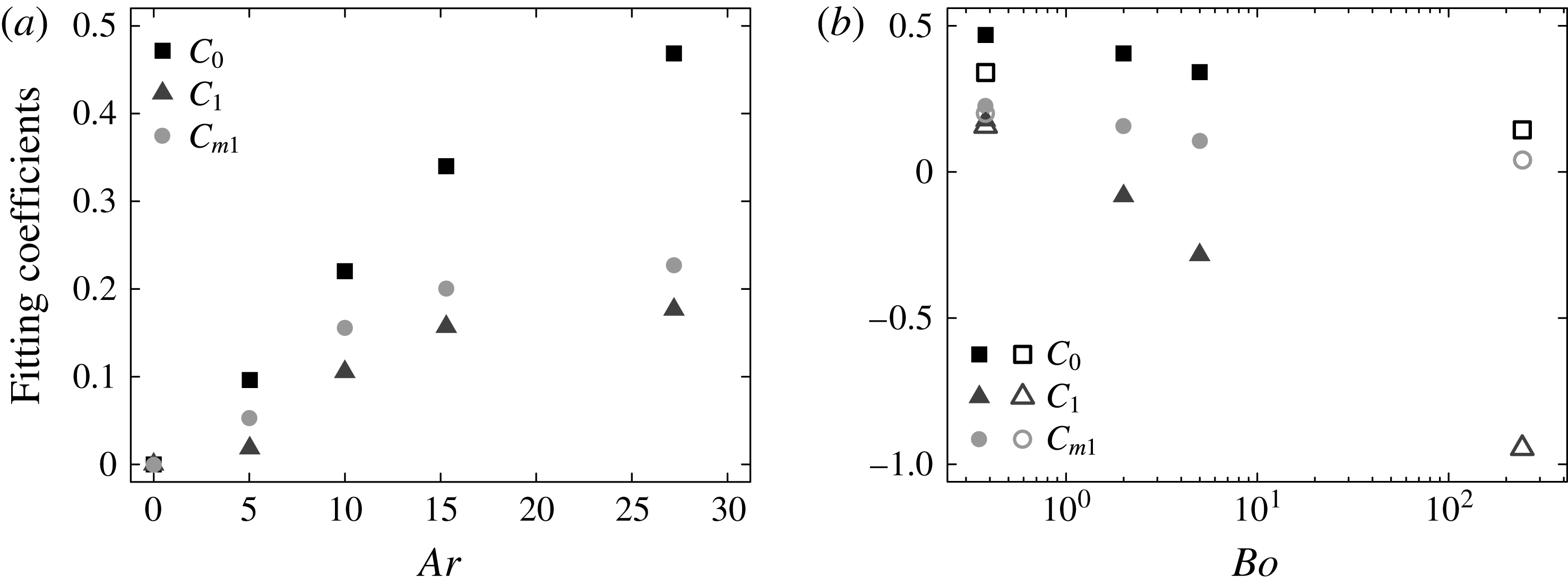
 $$\begin{eqnarray}\frac{U}{U_{0}}=1+\frac{U_{0,Stokes}}{U_{0}}\unicode[STIX]{x1D707}^{\ast }\frac{C_{0}-(1.1734+C_{1})\unicode[STIX]{x1D719}^{1/3}}{1+C_{m1}\unicode[STIX]{x1D719}^{-1/3}},\end{eqnarray}$$
where
 $U_{0,Stokes}$
is given by (4.2). We have introduced in this expression three fitting parameters
 $C_{0}$
,
 $C_{1}$
and
 $C_{m1}$
that we have computed for each case by a least-squares fit of DNS data at finite volume fraction and isolated-bubble data at zero volume fraction. The fitted values are shown in figure 9. These parameters account for the effect of inertial interactions (they are zero in the Stokes flow regime,
 $\mathit{Ar}=0$
), and are monotonic functions (increasing and decreasing, respectively) of the Archimedes and Bond numbers. The fitted expression of the normalized drift velocity is shown with dashed lines for each case in figure 3(b), figure 4 and figure 8, which show that the effect of volume fraction is well described by this law for all the flow regimes considered.
Fitted coefficients for
 $U(\unicode[STIX]{x1D719})/U_{0}$
as given by (4.8): (a) as a function of the Archimedes number for
 $\mathit{Bo}=0.38$
, (b) as a function of the Bond number for
 $\mathit{Ar}\approx 15$
(open symbols) and for
 $\mathit{Ar}\approx 30$
(filled symbols). The coefficients are obtained by least-squares fits of DNS and isolated-bubble data.

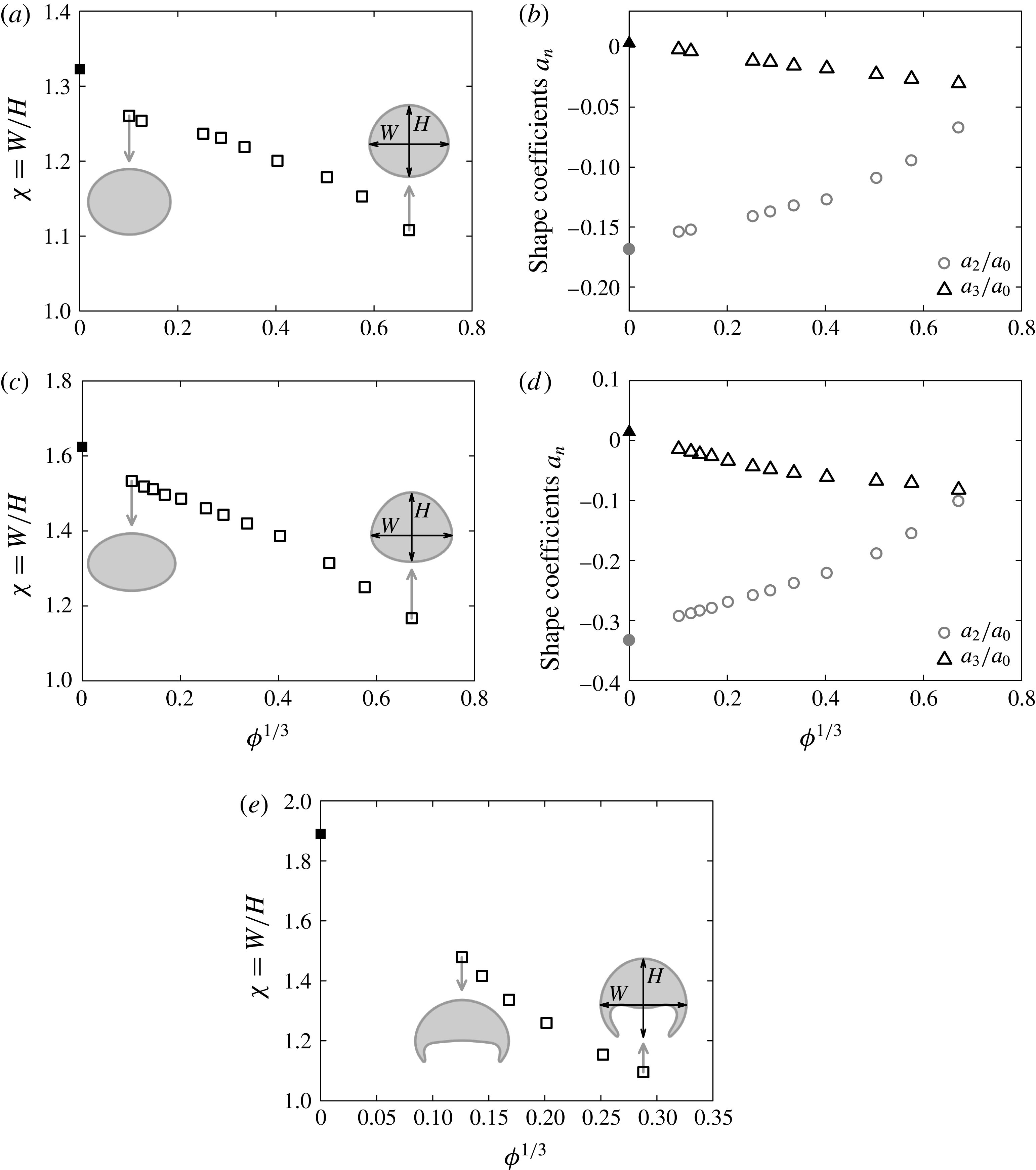
Steady aspect ratio (a,c,e) and shape coefficients (b,d) of bubbles in an ordered array configuration as a function of volume fraction for: (a,b) case E1 (
 $\mathit{Bo}=2.0$
,
 $\mathit{Ar}=29.9$
); (c,d) case E2 (
 $\mathit{Bo}=5.0$
,
 $\mathit{Ar}=30.0$
); (e) case C (
 $\mathit{Bo}=243$
,
 $\mathit{Ar}=15.2$
). Bubble shapes are shown in grey for the highest and the lowest simulated volume fractions. Open symbols: DNS. Filled symbol: isolated bubble (aspect ratios estimated from Loth (Reference Loth2008) for cases E1 and E2 and from Hua et al. (Reference Hua, Stene and Lin2008) for case C; shape coefficients estimated from Ryskin & Leal (Reference Ryskin and Leal1984)).

We now investigate the bubbles’ shape. At low
 $\mathit{Bo}$
(not shown here), the bubbles remain approximately spherical as volume fraction is varied; the aspect ratio
 $\unicode[STIX]{x1D712}$
(the maximum bubble width
 $W$
divided by the maximum bubble height
 $H$
, see figure 10) does not deviate from 1 by more than 5 %, due to the low value of the Weber number. At
 $\mathit{Bo}\geqslant O(1)$
, the bubble shape strongly depends on volume fraction, and is investigated below. For intermediate Reynolds numbers, say
 $1<\mathit{Re}<100$
, no theoretical expression of
 $\unicode[STIX]{x1D712}$
is available. At low
 $\mathit{Re}$
and
 $\mathit{We}$
a theoretical result is available (Taylor & Acrivos Reference Taylor and Acrivos1964) for the shape modes introduced below, but this has been found not to predict accurately results of numerical simulations for an isolated bubble if
 $\mathit{We}$
is increased to unity (Ryskin & Leal Reference Ryskin and Leal1984). The analysis by Moore (Reference Moore1959) is for values of
 $\mathit{Re}$
well over
 $100$
. Therefore, as a starting point in the following, the results of numerical simulations of an isolated bubble by Ryskin & Leal (Reference Ryskin and Leal1984) are used.
We first focus on ellipsoidal bubbles (cases E1 and E2). (The denomination ‘ellipsoidal bubble’ refers to a bubble that is approximately spheroidal with weak fore-and-aft asymmetry, but does not mean that the bubble shape is strictly ellipsoidal.) In all the simulations reported here, bubbles are virtually axisymmetric, but may exhibit significant fore-and-aft asymmetry. In figure 10, we present the aspect ratio as a function of volume fraction for these cases. Also shown are the first two shape coefficients
 $a_{2,3}$
defined by writing the local bubble radius
 $R(\unicode[STIX]{x1D703})$
as
 $$\begin{eqnarray}R(\unicode[STIX]{x1D703})=\mathop{\sum }_{n}a_{n}P_{n}(\cos \unicode[STIX]{x1D703}),\end{eqnarray}$$
where
 $P_{n}$
is the Legendre polynomial of order
 $n$
and
 $\unicode[STIX]{x1D703}$
is the angle between the position vector at the bubble surface and the bubble velocity (
 $a_{0}$
is the radius of the sphere with the same volume). The coefficients were obtained from a distribution of points (at least
 $500$
) on the bubble surface and integrating the orthogonality relation for each Legendre polynomial.
In figure 10(a–d), for both cases E1 and E2, as the volume fraction is increased,
 $\unicode[STIX]{x1D712}$
decreases monotonically to unity and
 $a_{2}$
goes to zero, from approximately their respective values for isolated bubbles. The corresponding single bubbles (for which results are shown in the figure with filled symbols, with shape coefficients obtained from Ryskin & Leal (Reference Ryskin and Leal1984)), are of oblate-ellipsoid shape. This shape is expected for isolated bubbles at large
 $\mathit{Re}$
, through a Bernoulli suction effect in the vicinity of the bubble rim, and is expected also at low
 $\mathit{Re}$
(Taylor & Acrivos Reference Taylor and Acrivos1964). It may be anticipated that the demise of this shape at elevated volume fraction is partly due to the dependencies of
 $\mathit{Re}$
and
 $\mathit{We}$
on volume fraction. We have verified, however, that the empirical correlation by Loth (Reference Loth2008) for the aspect ratio of isolated bubbles, using the values of these dimensionless groups obtained from the simulations, although yielding good agreement at
 $\unicode[STIX]{x1D719}=0$
gives a very poor prediction of the results presented in figure 10 (and is therefore not shown). The reduction of suction at the bubble rim is therefore due to the detailed bubble interactions. In their study of the hydrodynamic interactions between two spherical bubbles rising side by side, Legendre et al. (Reference Legendre, Magnaudet and Mougin2003) showed that at small to moderate Reynolds number (
 $\mathit{Re}\lesssim 30$
, as encountered in our study), the transverse force is repulsive and increases when the separation decreases. Such a reduction or elimination of suction between bubbles suggests the liquid downflow due to a bubble pair occurs around the pair as a whole. In a three-dimensional cubic array, although the room for liquid to flow down with little opposition is reduced further (at four sides along a bubble rim), some remains present along vertical edges of each cell in the array. Therefore, any suction effect normally arising at the rim of a bubble would be reduced in between bubbles lying in the same horizontal plane. This may be somewhat countered by an increase elsewhere along the bubble periphery (if not at a greater distance from the bubble), but a variation in curvature is opposed by surface tension.
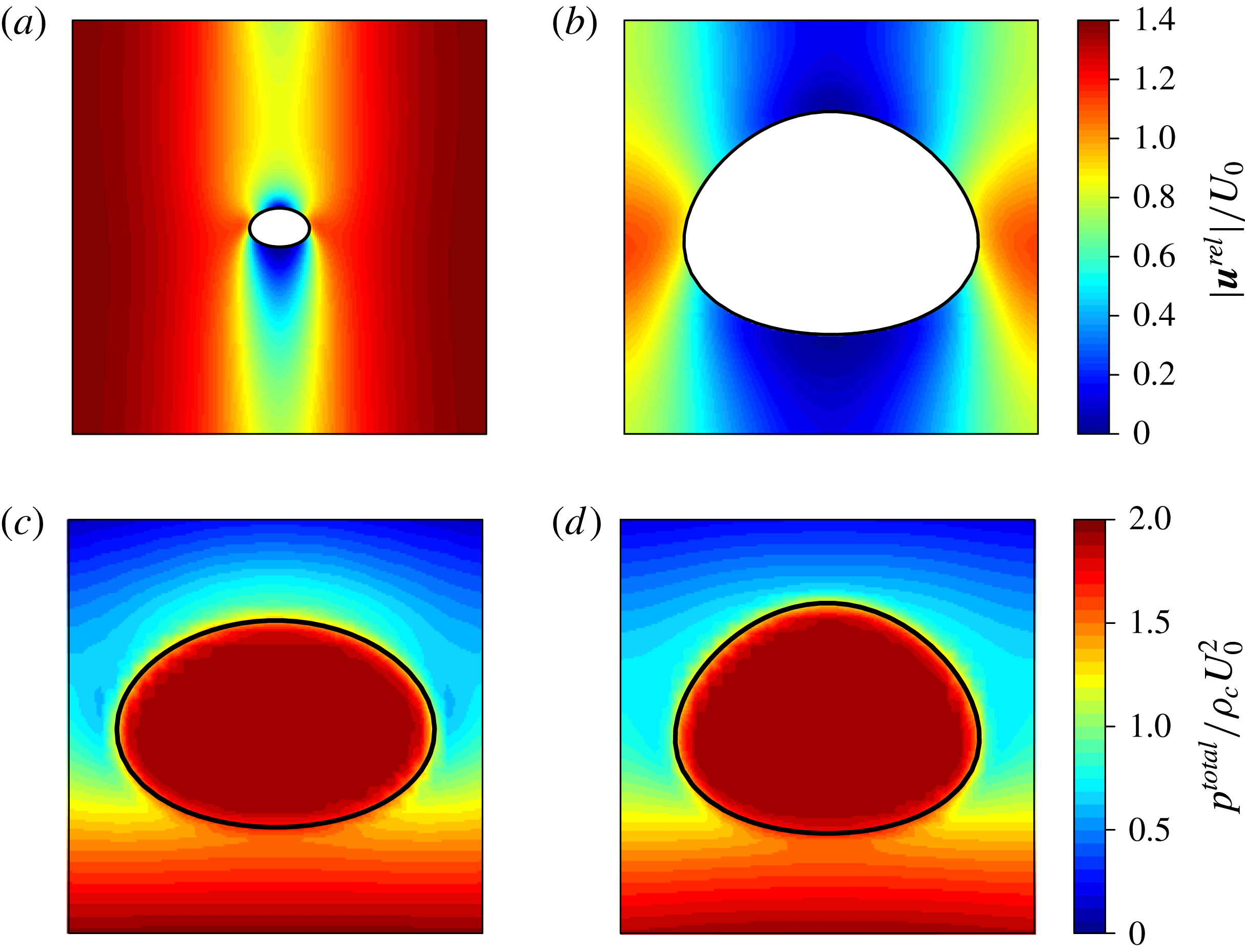
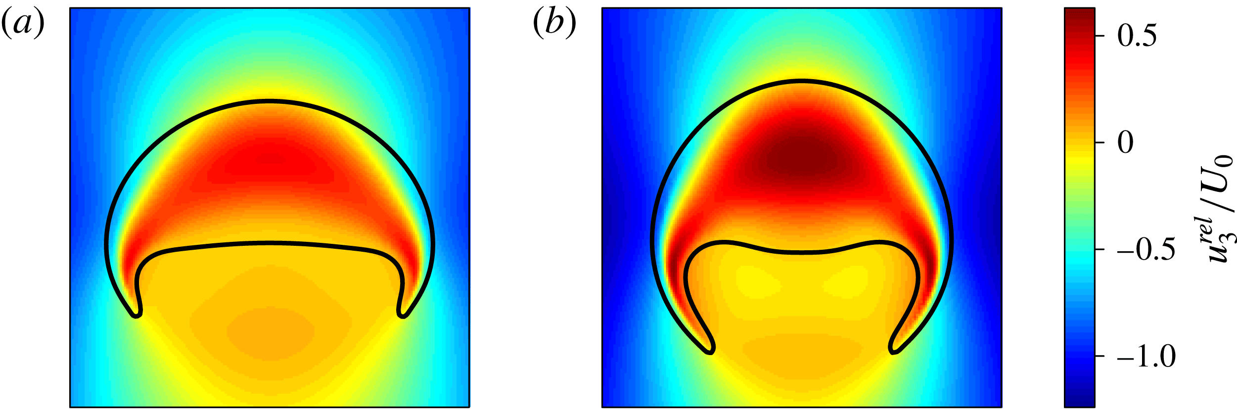
Influence of volume fraction on the deformation of an ordered array of oblate ellipsoidal bubbles (case E2): relative velocity (
 $\boldsymbol{u}^{\text{rel}}=\boldsymbol{u}-\langle \boldsymbol{u}\rangle _{d}$
) and pressure fields in a vertical symmetry plane passing through the centre of a bubble. Increasing volume fractions from left to right: (a,c)
 $\unicode[STIX]{x1D719}=0.1$
%,
 $U/U_{0}=1.34$
and (b,d)
 $\unicode[STIX]{x1D719}=13$
%,
 $U/U_{0}=0.73$
. (a,b) Magnitude of the liquid relative velocity in the entire unit cell. (c,d) Total pressure (including the mixture-average hydrostatic component) near and inside a bubble. Gravity is pointing downward (
 $\boldsymbol{g}=-g\boldsymbol{e}_{3}$
). The black lines show the interface location.

In addition to this reduction in aspect ratio, the fore-and-aft asymmetry of the shape of an isolated bubble is altered significantly by the finite volume fraction. For single bubbles, cases E1 and E2 are near the boundary between a low-
 $\mathit{Re}$
regime of bubbles with a blunt tail and, at the same
 $\mathit{We}$
but larger
 $\mathit{Re}$
, a regime of bubbles with a flat nose (Ryskin & Leal Reference Ryskin and Leal1984); only a slightly flattened nose is observed, mostly in case E2, resulting in a positive value of
 $a_{3}$
in (4.9). The results in figure 10(b,d) show that already at small but finite volume fraction this asymmetry is reversed. The bubble nose becomes rather pointed and the tail blunt as the volume fraction is increased further. This tendency for oblate ellipsoidal bubbles arranged in regular arrays to have their nose pulled upwards at finite volume fraction has been observed previously by Sankaranarayanan et al. (Reference Sankaranarayanan, Shan, Kevrekidis and Sundaresan2002), and attributed to a wake effect. Indeed Hallez & Legendre (Reference Hallez and Legendre2011) showed that in the present range of Reynolds numbers, two spherical bubbles rising in line are attracted toward each other for separation distances greater than approximately 1.3 bubble diameter, which would be equivalent to
 $\unicode[STIX]{x1D719}^{1/3}=0.62$
, a value close to the upper bound of the range of volume fractions we consider. To investigate this further, the amplitude of the
 $P_{3}$
mode in (4.9) is included in figure 10. It is seen that in concentrated arrays this becomes as significant as that of the
 $P_{2}$
mode. The presence of successive bubbles in each other’s wakes does reduce the variation in velocity magnitude between them, as can be seen in figure 11(a,b). The significance of the stagnation-point flow at the bubble nose is thereby reduced as volume fraction is increased, and the large dynamic pressure at a stagnation point in the liquid is reduced (the pressure field is shown in figure 11
c,d), along with the magnitude of normal deviatoric stress. Both these result in an increase in the jump in normal stress and hence an increase in interface curvature.
Finally we note that the results for aspect ratio and shape coefficients for cases E1 and E2 differ by a factor of approximately two, which roughly corresponds to the ratio of the bubble Weber numbers at all volume fractions. As we have not undertaken to extend our parametric study even further to confirm, it is concluded that the results for
 $(\unicode[STIX]{x1D712}-1)$
and
 $a_{2,3}$
versus Weber number, in the present range of
 $\mathit{We}<7$
, are consistent with a linear dependency.
We have also investigated a regime characterized by a very high Bond number (case C,
 $\mathit{Bo}=243$
). The evolution of the bubbles’ ‘aspect ratio’ and shape with volume fraction is shown in figure 10(e). The corresponding bubbles in isolation are indented ellipsoidal caps (Bhaga & Weber Reference Bhaga and Weber1981; Hua et al.
Reference Hua, Stene and Lin2008). As the volume fraction increases, the upside-down crown of gas issuing from the bubble rim becomes thinner and longer to form a skirt with an inward curvature (in the direction of the bubble axis of symmetry). The range of
 $\unicode[STIX]{x1D719}$
values that can be considered in this case is relatively narrow, since for
 $\unicode[STIX]{x1D719}\gtrsim 6$
% the bubbles become so elongated that they coalesce.
The theory of Ray & Prosperetti (Reference Ray and Prosperetti2014) indicates that the finite length of the skirt is dictated by the thinning of the skirt downstream of its point of formation. According to their model, the skirt thickness is proportional to
 $\sqrt{-u_{s}}$
, where
 $u_{s}$
is the (negative) vertical component of the relative velocity (that is, the liquid velocity in the bubble’s frame of reference) at the outer side of the skirt at a given altitude (the inward curvature of the skirt being neglected). We show in figure 12 the vertical relative velocity
 $u_{3}^{\text{rel}}=u_{3}-\langle u_{3}\rangle _{d}$
in the vicinity of bubble (with gravity pointing in the
 $-\boldsymbol{e}_{3}$
direction). It can be observed that as the distance from the rim increases,
 $|u_{s}|$
(
 $|u_{3}^{\text{rel}}|$
along the outer side of the skirt) decreases and the skirt tapers, until the skirt ends for a critical value of
 $|u_{s}|$
, in (qualitative) agreement with the model of Ray & Prosperetti (Reference Ray and Prosperetti2014). By comparing figure 12(a) with figure 12(b) one remarks that at high volume fractions a significant downflow of liquid develops outside of bubbles’ wakes. This backflow of liquid, which is particularly strong because the bubbles rise velocity is not substantially reduced for large values of
 $\unicode[STIX]{x1D719}$
, increases the value of
 $|u_{s}|$
at a given altitude. Therefore, at higher volume fraction, the skirt must extend further downstream to reach the critical value of
 $|u_{s}|$
at which the skirt ends, as observed in our simulations.
Influence of volume fraction on the deformation of an ordered array of dimpled ellipsoidal-cap bubbles (case C): vertical component of the relative velocity (
 $\boldsymbol{u}^{rel}=\boldsymbol{u}-\langle \boldsymbol{u}\rangle _{d}$
) in a vertical symmetry plane passing through the centre of a bubble. Increasing volume fractions from left to right: (a)
 $\unicode[STIX]{x1D719}=0.2$
%,
 $U/U_{0}=1.22$
, and (b)
 $\unicode[STIX]{x1D719}=2.4$
%,
 $U/U_{0}=1.17$
. Same conventions as in figure 11. Only the region near and inside a bubble is shown.

The aspect ratio of the skirted bubble decreases towards unity as the volume fraction is increased, even if the skirt is not included in the height. Indeed, given the moderate value of the Reynolds number (
 $\mathit{Re}\approx 10$
), the same reasoning as above for ellipsoidal bubbles is expected to apply, that is, a decrease of the suction effect as the size of the gap between side neighbours decreases. At low volume fraction, an extrapolation of the results to zero volume fraction appears consistent with the corresponding result for a single bubble.
4.2 Steady and unsteady oblique rise of bubbles
In the range of parameters considered thus far, the motion of a single bubble in unbounded liquid is straight, steady and parallel to gravity. For cases E1 and S5, an oblique (i.e. not aligned with gravity) bubble motion was, however, observed at certain volume fractions. Such oblique motions have been reported previously for two-dimensional square arrays of bubbles (Sankaranarayanan et al.
Reference Sankaranarayanan, Shan, Kevrekidis and Sundaresan2002; Sankaranarayanan & Sundaresan Reference Sankaranarayanan and Sundaresan2002; Theodoropoulos et al.
Reference Theodoropoulos, Sankaranarayanan, Sundaresan and Kevrekidis2004), but their triggering and their stability remain essentially unexplained. We analyse oblique rise further here. In this subsection the bubble drift velocity vector is denoted by
 $\boldsymbol{U}=U_{i}\boldsymbol{e}_{i}$
and the gravity vector by
 $\boldsymbol{g}=-g\boldsymbol{e}_{3}$
, where
 $\boldsymbol{e}_{i}$
are the unit primary vectors of the periodic array.
First, existence of such oblique solutions is demonstrated at Reynolds numbers that are small but finite. The Oseen analysis in appendix B yields the system of equations (B 3) that involve the bubble velocity and the force exerted by the fluid on the bubble. As this force is prescribed (it balances buoyancy), equation (B 3) yields the bubble velocity. The main solution is naturally a velocity vector aligned with gravity, as studied in § 4.1. Equation (B 3) does, however, allow for other solutions which satisfy the nonlinear system of equations (B 12). We have found these non-trivial solutions at values of
 $\mathit{Ar}$
around 20. The most convenient way to obtain these solutions was found to be, for a given inclination of the bubble velocity (with respect to the upward vertical direction), to reduce the problem to a single nonlinear equation for the Reynolds number based on the lattice spacing and the magnitude of the bubble velocity (
 $\mathit{Re}_{h}$
in the Appendix), and to obtain the volume fraction from the remainder of the system of equations. Two types of non-trivial solutions were studied: either the horizontal bubble velocity component was aligned with one of the lattice unit vectors or it was diagonal to the lattice. The results are presented in figure 13. It is seen that these exist below a critical value of the volume fraction (which we have found to increase rapidly with the value of
 $\mathit{Ar}$
), the inclination angle strongly increasing as the volume fraction is reduced. Oblique rise of single light solid particles has already been observed in numerical simulations (Jenny, Dusek & Bouchet Reference Jenny, Dusek and Bouchet2004) and experiments (Veldhuis & Biesheuvel Reference Veldhuis and Biesheuvel2007), also arising as a non-trivial further solution (Fabre, Tchoufag & Magnaudet Reference Fabre, Tchoufag and Magnaudet2012), but the present solutions crucially involve bubble interactions, we investigate this further below.
Subset of analytical solutions obtained from solving (B 3) for
 $\mathit{Ar}=20$
and
 $\unicode[STIX]{x1D70C}_{d}/\unicode[STIX]{x1D70C}_{c}=\unicode[STIX]{x1D707}_{d}/\unicode[STIX]{x1D707}_{c}=0$
: bubble drift velocity horizontal (a) and vertical (b) components, given as Reynolds numbers
 $\mathit{Re}_{i}=U_{i}\unicode[STIX]{x1D70C}_{c}d_{b}/\unicode[STIX]{x1D707}_{c}$
, as a function of volume fraction. Gravity is pointing in the
 $-\boldsymbol{e}_{3}$
direction.
 $\cdots \cdots$
, vertical rise (
 $U_{1}=U_{2}=0$
); – – – –, oblique rise with
 $U_{2}=0$
; ——, oblique rise with
 $|U_{2}|=|U_{1}|$
.

We now return to numerical results. After an initial transient during which they accelerate from rest under the effect of buoyancy, the bubbles may be deflected from their original vertical trajectories. At this point, the horizontal components of the bubble velocity grow in magnitude while the rise velocity drops off. After that, velocity fluctuations set in. Three types of dynamic behaviours have been identified depending on the evolution of these fluctuations: (i) the fluctuations may rapidly dampen out, and the bubbles finally rise steadily on a straight (but skewed to gravity) path; (ii) they may take the form of oscillations, so that the bubbles’ motion is oscillatory around a straight oblique path; or (iii) they may become aperiodic, so the bubble rise is chaotic and, on average, not aligned with gravity. These regimes are exemplified in figure 14, and will be respectively referred to as steady oblique rise (a,b), oscillatory oblique rise (c) and chaotic oblique rise (d).
Time signals of the bubble drift velocity components (given as Reynolds numbers
 $\mathit{Re}_{i}=\unicode[STIX]{x1D70C}_{c}U_{i}d_{b}/\unicode[STIX]{x1D707}_{c}$
), with
 $\boldsymbol{U}=U_{i}\boldsymbol{e}_{i}$
and gravity pointing in the
 $-\boldsymbol{e}_{3}$
direction, in the three regimes of motion: steady oblique rise (a,b), oscillatory oblique rise (c) and chaotic oblique rise (d). These regimes are obtained for (a) case E1 at
 $\unicode[STIX]{x1D719}=0.8$
%, (b) case S5 at
 $\unicode[STIX]{x1D719}=13$
%, (c) case S5 at
 $\unicode[STIX]{x1D719}=3.8$
%, (d) case S5 at
 $\unicode[STIX]{x1D719}=0.5$
%.

The bubble drift velocities are in all cases either steady or statistically stationary, so mean drift velocities can be defined by averaging over a sufficient time period. The horizontal and vertical components of the (statistically) steady drift velocity are plotted against volume fraction in figure 15 for cases E1 and S5. Filled symbols are used for steady bubble motion, vertical or oblique. For unsteady bubble motion, the time-averaged drift velocity is shown with open symbols, and the standard deviation is represented using vertical bars. In case E1 (figure 15
a), steady vertical rise is obtained at low and high volume fractions, whereas at intermediate volume fractions the bubbles rise steadily along an oblique path with an inclination angle of approximately
 $3^{\circ }$
. This figure shows that three solutions exist in this regime: a symmetric vertical solution (
 $U_{1}=U_{2}=0$
) and two asymmetric oblique solutions consisting of horizontal velocity components of equal magnitude (
 $|U_{1}|=|U_{2}|\neq 0$
), as predicted from the Oseen flow analysis (figure 13). In case S5 (figure 15
b), steady vertical rise, steady oblique rise, oscillatory oblique rise and chaotic oblique rise are obtained in that order as volume fraction is decreased. Inclination of the velocity with respect to the upward vertical direction is between
 $6^{\circ }$
and
 $13^{\circ }$
(maximum for
 $\unicode[STIX]{x1D719}^{1/3}=0.4$
). As volume fraction approaches zero, the steady vertical rise of the isolated bubble must be recovered, although the occurrence of this transition cannot be evidenced by numerical simulations owing to their prohibitive cost.
Quasi-steady drift velocity components (
 $\boldsymbol{U}=U_{i}\boldsymbol{e}_{i}$
) in the form of Reynolds numbers (
 $\mathit{Re}_{i}=\unicode[STIX]{x1D70C}_{c}U_{i}d_{b}/\unicode[STIX]{x1D707}_{c}$
) as a function of volume fraction for an ordered array of bubbles in the cases where bubbles exhibit non-vertical motions. Gravity is pointing in the
 $-\boldsymbol{e}_{3}$
direction. (a) Case E1 (
 $\mathit{Bo}=2.0$
,
 $\mathit{Ar}=29.9$
, note that the horizontal components have been multiplied by 10 for clarity). (b) Case S5 (
 $\mathit{Bo}=0.38$
,
 $\mathit{Ar}=40.7$
). Filled symbols are used when the bubbles’ motion is steady (oblique or vertical). Open symbols and vertical bars are used when the bubbles’ motion is unsteady: symbols indicate the mean drift velocity, and bars show its root mean square. The dashed line is a numerical fit of the form of (4.8) matching DNS and isolated-bubble data for the vertical rise only.

It is possible to obtain insight into this behaviour by using prior results for bubble pairs. At steady state, the integral of fluid stresses over the bubble surface, denoted by
 $\boldsymbol{f}$
, is balanced by the buoyancy force
 $\boldsymbol{f}_{buoy}$
:
 $\boldsymbol{f}=-\boldsymbol{f}_{buoy}$
, with
 $\boldsymbol{f}_{buoy}=f_{buoy}\boldsymbol{e}_{3}=(\unicode[STIX]{x03C0}/6)d_{b}^{3}(\unicode[STIX]{x1D70C}_{c}-\unicode[STIX]{x1D70C}_{d})g\boldsymbol{e}_{3}$
. The total surface force
 $\boldsymbol{f}$
acting on the bubble can be decomposed into a drag force
 $\boldsymbol{f}_{drag}$
and a lift force
 $\boldsymbol{f}_{lift}$
, defined by
 $$\begin{eqnarray}\boldsymbol{f}_{drag}=(\boldsymbol{f}\boldsymbol{\cdot }\boldsymbol{U})\frac{\boldsymbol{U}}{|\boldsymbol{U}|^{2}},\quad \boldsymbol{f}_{lift}=\boldsymbol{f}-\boldsymbol{f}_{drag},\end{eqnarray}$$
and corresponding to longitudinal and transverse components of
 $\boldsymbol{f}$
with respect to the direction of motion, respectively (these definitions can be used for unsteady but statistically stationary systems by replacing
 $\boldsymbol{U}$
and
 $\boldsymbol{f}$
by their time averages). The persistence of a (possibly average) oblique motion implies the existence of a net (average) lift force exerted on the bubble. The magnitude of this lift force is classically presented in the form of a dimensionless lift coefficient
 $C_{L}$
defined by
 $$\begin{eqnarray}C_{L}=\frac{|\boldsymbol{f}_{lift}|}{0.125\unicode[STIX]{x03C0}d_{b}^{2}\unicode[STIX]{x1D70C}_{c}|\boldsymbol{U}|^{2}}.\end{eqnarray}$$
The (average) lift coefficient is plotted as a function of volume fraction in figure 16 for case E1 (open grey triangles) and case S5 (open black squares).
Since the tilt angle remains small (not larger than
 $13^{\circ }$
in our simulations), each bubble is in the wake of its predecessor, and the oblique path is expected to originate from the vorticity produced by the preceding bubble. We therefore investigate whether the lift force induced by the preceding bubble can be estimated from prior work on bubble pairs separated by a fixed distance equal to the present lattice spacing, both rising at a constant velocity
 $\boldsymbol{U}$
and where the angle between
 $\boldsymbol{U}$
and the vertical line joining their centres is the inclination angle measured from our simulations. The model proposed by Hallez & Legendre (Reference Hallez and Legendre2011) for bubble pairs ((6.12) therein) is used here for this purpose. A spherical bubble shape appears a reasonable approximation given that in our simulations the aspect ratio does not exceed 1.3 for case E1, and 1.1 for case S5. The results are shown in figure 16 with larger filled symbols. To assess the influence of the leading bubble’s wake, the lift coefficient obtained for bubble pairs without the contribution from the wake is shown on the same figure with smaller filled symbols. The trend obtained by considering the pair interaction is in excellent adequacy with our numerical results for periodic arrays when the wake of the top bubble is accounted for, thereby demonstrating that oblique rise is essentially a wake-induced effect. The lift coefficient in ordered suspensions is found to be larger than that due to the interaction with the wake of a single bubble, and the difference is more pronounced at higher volume fractions, since in the periodic configuration the bubble has an infinite number of top neighbours that may contribute to the lift force.
Average lift coefficient as a function of volume fraction for case E1 (grey triangles) and case S5 (black squares). Open symbols: for a bubble of an ordered array, present DNS. Filled symbols: for the trailing bubble of a pair of spherical bubbles within the same conditions (orientation, Reynolds number, separation distance) as two vertically aligned bubbles of the ordered array, with (large symbols) and without (small symbols) accounting for the interaction with the wake of the leading bubble, from Hallez & Legendre (Reference Hallez and Legendre2011).

This reasoning can even be made more precise by considering the expression of the lift force acting on a single spherical bubble moving in a (e.g. wake-induced) rotational flow (Auton Reference Auton1987; Legendre & Magnaudet Reference Legendre and Magnaudet1998; Hallez & Legendre Reference Hallez and Legendre2011):
 $$\begin{eqnarray}\boldsymbol{f}_{lift}\propto d_{b}^{3}\unicode[STIX]{x1D70C}_{c}\unicode[STIX]{x1D734}\times \boldsymbol{U}.\end{eqnarray}$$
In this expression,
 $\unicode[STIX]{x1D734}=|\unicode[STIX]{x1D734}|\boldsymbol{e}_{h}$
is the liquid vorticity ‘seen’ by the bubble and produced by the motion of all the other bubbles. No clear definition of this quantity is available if vorticity is not uniform at the bubble scale, as is the case in the present study, but it is reasonable to assume that it can be qualitatively estimated by examining vorticity profiles in the bubble vicinity. In turbulent flows, Merle, Legendre & Magnaudet (Reference Merle, Legendre and Magnaudet2005) and Naso & Prosperetti (Reference Naso and Prosperetti2010) approximated the velocity and vorticity ‘seen’ by bubbles and solid particles respectively, by the average of these quantities over shells of different sizes. In order to show that our results are qualitatively consistent with (4.12), it is thus convenient to introduce an orthonormal direct basis
 $(\boldsymbol{e}_{\Vert },\boldsymbol{e}_{\bot },\boldsymbol{e}_{h})$
, defined by the unit vectors
 $$\begin{eqnarray}\boldsymbol{e}_{\Vert }=\frac{\boldsymbol{U}}{|\boldsymbol{U}|},\quad \boldsymbol{e}_{\bot }=\frac{\boldsymbol{f}_{lift}}{|\boldsymbol{f}_{lift}|},\quad \boldsymbol{e}_{h}=\boldsymbol{e}_{\Vert }\times \boldsymbol{e}_{\bot }.\end{eqnarray}$$
The bubble’s steady motion is contained in the vertical plane defined by
 $(\boldsymbol{e}_{\Vert },\boldsymbol{e}_{\bot })$
. We now examine the sign and magnitude of the liquid vorticity component
 $\unicode[STIX]{x1D714}_{h}=\unicode[STIX]{x1D74E}\boldsymbol{\cdot }\boldsymbol{e}_{h}$
ahead of the bubble, where it should overall give a positive contribution to
 $|\unicode[STIX]{x1D734}|$
for the above model to be correct. We show in figure 17 the liquid vorticity field projected onto
 $\boldsymbol{e}_{h}$
in the vertical plane normal to
 $\boldsymbol{e}_{h}$
for two examples of steady oblique rise. The bubble in figure 17(b) experiences a stronger lift force (indicated by the thick orange arrow) than the bubble in figure 17(a). This is consistent with (4.12) and the fact that, upstream of the bubble (its drift velocity being shown with the black arrow),
 $\unicode[STIX]{x1D714}_{h}$
is positive and its magnitude is larger than that in figure 17(a) (although only two examples are shown here the same result holds for all our simulations). In addition it is seen from figure 17 that
 $\unicode[STIX]{x1D714}_{h}$
is transported from the surface of preceding bubbles, hence confirming the key role played by the wakes and the associated lift force for the stability of oblique motion.
Liquid vorticity horizontal component
 $\unicode[STIX]{x1D714}_{h}=\unicode[STIX]{x1D74E}\boldsymbol{\cdot }\boldsymbol{e}_{h}$
in the vertical plane passing through the centre of a bubble and containing its drift velocity, for ordered arrays of bubbles rising steadily in an oblique direction: (a) case E1,
 $\unicode[STIX]{x1D719}=0.8$
%; (b) case S5,
 $\unicode[STIX]{x1D719}=6.5$
%. Positive (negative) values upstream of the bubble would give a positive (negative) contribution to the lift force as modelled by (4.12). The thin black arrow shows the direction of bubble drift velocity. The thick arrows show the magnitudes and directions of the drag (green arrows) and lift (orange arrows) forces scaled by the buoyancy force.

We will now examine the time dependence of bubble motions in the unsteady regimes. As illustrated in figure 18, which depicts the single-sided amplitude spectra of the discrete Fourier transforms of the drift velocity components time signals in the oscillatory (a) and chaotic (b) rise regimes, a spectral analysis of the unsteady velocity signals reveals clear peaks at a frequency equal to
 $f_{h}=(\overline{U}_{1}+\overline{U}_{2})/(2h)$
(where the bar denotes a time average). Normalizing frequencies by
 $f_{3}\equiv \overline{U}_{3}/h$
(not shown here) does not lead to a collapse of the curves. This suggests that the force fluctuations experienced by a bubble are also driven by the interaction with the wakes of the preceding bubbles that are not on the same vertical axis. As a consequence, the dynamic behaviour of a bubble in an ordered array, although greatly influenced by the direct interaction with its top neighbour, is also dictated by longer-range nonlinear interactions with other bubbles located in above horizontal planes.
Single-sided amplitude spectra of discrete Fourier transforms of the drift velocity components time signals. Unsteady oblique rise of ordered arrays of bubbles: (a) oscillatory motion (case S5 at
 $\unicode[STIX]{x1D719}=3.8$
%), (b) chaotic motion (case S5 at
 $\unicode[STIX]{x1D719}=1.6$
%). The amplitude is normalized by the average vertical drift velocity
 $\overline{U}_{3}$
, and the frequency is normalized by
 $f_{h}=(\overline{U}_{1}+\overline{U}_{2})/(2h)$
.

In the light of these results, we are now in a position to propose the following scenario for explaining the transitions between the various regimes of motion reported in figure 15. First, non-vertical motion can only occur when the flow conditions allow sufficiently high Reynolds numbers to be attained (here, cases E1 and S5). Vorticity then becomes significant in the vicinity of each bubble due to the wake of its predecessor; an infinitesimal asymmetry can then result in a lift force that is sufficient to result in oblique motion (Koch Reference Koch1993). If each bubble is only influenced by the wake of its immediate predecessor, this motion is steady. When the wakes extend horizontally over distances large compared to the lattice spacing, each bubble interacts with the wakes of a great number of neighbours, including some that are not located on the same vertical axis, and the motion becomes chaotic. Then, for a given flow regime, the volume fraction is in the first place related to the distance between the bubbles, but also affects the Reynolds number in a non-monotonic manner. At low volume fraction, when the Reynolds number increases with volume fraction, steady vertical rise, steady oblique rise and unsteady oblique rise occur in that order at increasing volume fraction. At higher volume fraction, the situation becomes more complex because the Reynolds number decreases with
 $\unicode[STIX]{x1D719}$
. It appears that the dominant effect of increasing volume fraction is then not to bring the bubbles closer to each other, but to reduce their velocity, so that steady oblique rise is first recovered, and is replaced by steady vertical rise at the highest volume fractions.
5 Free arrays
We examine in this section the behaviour of freely evolving bubbly flows as represented by the repetition of a unit cell containing several independent bubbles (‘free arrays’). This problem, studied previously by several groups (e.g. Bunner & Tryggvason Reference Bunner and Tryggvason2002a ; Esmaeeli & Tryggvason Reference Esmaeeli and Tryggvason2005; Yin & Koch Reference Yin and Koch2008) but only at moderate and high volume fractions, is revisited here following the insights gained in the previous section for ordered arrays. Our main objective in this section is to investigate the dynamics of free arrays at small and intermediate volume fractions, and to compare the observed trends with those obtained for ordered suspensions.
Simulations of free arrays of bubbles have been undertaken for cases E1 and C (table 1). The two fluids were initially at rest,
 $N_{b}$
identical spherical bubbles were introduced in a cubic periodic unit cell of size
 $h$
(which results in a gas volume fraction
 $\unicode[STIX]{x1D719}=(\unicode[STIX]{x03C0}N_{b}d_{b}^{3})/(6h^{3})$
) and gravity was switched on at time zero. It was found that the transient evolution of the system can follow either of two routes: one with successive pair coalescence events until an ordered array configuration is recovered, and the other one in which the number of bubbles remains constant throughout the simulation. The former was observed for case C, which corresponds to highly deformable bubbles of dimpled or skirted ellipsoidal-cap shapes, even at relatively low volume fractions (the lowest volume fraction considered in that case was
 $\unicode[STIX]{x1D719}=0.8$
%). In case E1 (weakly ellipsoidal bubbles), by contrast, coalescence was never observed, provided that the bubbles’ interfaces are initially sufficiently separated from each other and that the volume fraction remains below approximately 5 % (we shall elaborate on this last point in § 5.2). Examination of the suspension evolution revealed that bubbles never come into close contact in that case, as previously observed by Esmaeeli & Tryggvason (Reference Esmaeeli and Tryggvason1999) in a similar flow regime. After a transient regime, the flow was found to become independent of the initial bubbles’ positions and a well-defined statistically steady state was reached.
In the following we analyse the statistically stationary rise of free, non-coalescing, deformable bubbles at moderate Reynolds number (case E1). Approximately 50 simulations of free arrays were run in total, corresponding to different initial conditions, numbers of bubbles and volume fractions. For each of these, the transient evolution of the system was monitored through the time signals of the bubble drift velocity
 $\boldsymbol{U}$
(defined, as for ordered arrays, by (2.3), and therefore equal to the average drift velocity of the
 $N_{b}$
bubbles) and of the interface surface area
 $A$
(which is a measure of the average deformation of the
 $N_{b}$
bubbles). In all simulations, the instantaneous horizontal components of
 $\boldsymbol{U}$
were found to be negligibly small, so we shall hereinafter simply use
 $U$
to denote the vertical component of the drift velocity vector. Each simulation was continued until
 $U$
and
 $A$
became statistically stationary. Their time averages, denoted by overbars in what follows, were then computed by averaging over a sufficient time interval.
5.1 Convergence with the number of bubbles
The influence of the number of free bubbles in the unit cell is evaluated by varying
 $N_{b}$
from 2 to 27 while keeping the volume fraction (and all other parameters) constant. The evolution of the bubbles’ drift velocity with the number of bubbles is shown in figure 19 for
 $\unicode[STIX]{x1D719}=2.4$
% (filled circles). The main effect of additional degrees of freedom is to slow down the bubbles: the drift velocity drops by 15 % when the relative motion between two bubbles is allowed, and is reduced further (up to
 ${\approx}30$
%) if the number of bubbles in the unit cell is increased. For
 $N_{b}\geqslant O(10)$
, the drift velocity becomes nearly independent of the number of bubbles. The rate of convergence and the maximal relative decrease in drift velocity with the number of bubbles appear to be essentially independent of the volume fraction, at least in the limited range considered here, as shown in figure 19 (open triangles and squares). The drift velocities obtained by Bunner & Tryggvason (Reference Bunner and Tryggvason2002a
) for a similar flow regime have been reported in the same figure (crosses). It is worth mentioning that although the maximum number of bubbles shown in figure 19 is
 $N_{b}=27$
, Bunner & Tryggvason (Reference Bunner and Tryggvason2002a
) have performed simulations for
 $1\leqslant N_{b}\leqslant 216$
(see figure 8a in their paper), and also concluded that the effect of the system size on the drift velocity becomes negligible for
 $N_{b}\geqslant O(10)$
in this flow regime. Overall the agreement between the two data sets is excellent, including in the peculiar case
 $N_{b}=4$
.
Influence of the number of bubble on the average bubble drift velocity for various volume fractions. The drift velocity is normalized by that obtained in the ordered configuration (
 $N_{b}=1$
). Symbols other than crosses: present DNS for case E1 (
 $\mathit{Ar}=29.9$
,
 $\mathit{Bo}=2.0$
). Crosses: prior DNS of Bunner & Tryggvason (Reference Bunner and Tryggvason2002a
) for a comparable flow regime (
 $\mathit{Ar}=29.7$
,
 $\mathit{Bo}=0.98$
).

It can indeed be noticed in figure 19 that convergence is not monotonic and that the rise is abnormally slow for
 $N_{b}=4$
. Visual inspection of the spatial distribution of the bubbles reveals a significant preference for horizontal alignment in that case. This bias is particularly pronounced for values of
 $\unicode[STIX]{x1D719}$
that are not very small and is therefore illustrated in figure 20 for
 $\unicode[STIX]{x1D719}=3.8$
%: while the bubbles are rather uniformly distributed within the periodic cell for
 $N_{b}=8$
(b), as is the case for other typical values of
 $N_{b}$
, they all remain in the same horizontal plane when
 $N_{b}=4$
(a), so that in the latter case the suspension actually consists of successive horizontal layers of bubbles. As shown by Hallez & Legendre (Reference Hallez and Legendre2011), side-by-side alignment maximizes the drag force acting on a pair of bubbles, resulting in lower drift velocities than with other types of spatial distributions.
Influence of the number of free bubbles on their spatial distribution within a periodic unit cell: typical instantaneous snapshots for
 $N_{b}=4$
(a) and
 $N_{b}=8$
(b), for case E1 at
 $\unicode[STIX]{x1D719}=3.8$
%.

This particular behaviour for
 $N_{b}=4$
demonstrates that an ordered microstructure is not always unstable. Such arrangements in horizontal planes are indeed possible if the number of free bubbles possesses an integer square root, due to periodicity and system symmetries. For
 $N_{b}=9$
, the bubbles also tend to arrange within a single horizontal plane, but this arrangement rapidly breaks up and is only observed intermittently. This results in the small but noticeable anomalous reduction of the drift velocity visible for
 $N_{b}=9$
in figure 19. For
 $N_{b}=16$
, no horizontal layer of bubbles is formed during the simulation and no anomaly is detectable in figure 19. We conclude that the artificial effects of symmetry and periodicity observed when
 $N_{b}$
is an exact square rapidly vanish as the number
 $N_{b}$
of independent bubbles is increased.
5.2 The effect of volume fraction on bubble drift velocity and deformation
The volume fraction has been varied from 0.2 % to 3.8 % by reducing the size of the unit cell while keeping all the other parameters constant, for a number of freely moving bubbles set to
 $N_{b}=8$
. For volume fractions greater than 5 %, numerical coalescence (that is, coalescence due to the spacing between bubble interfaces being less than the grid spacing) occurs during the transient evolution of the flow, therefore no data could be obtained for high volume fractions.
Data for fairly high volume fractions are however available from prior studies of Bunner & Tryggvason (Reference Bunner and Tryggvason2002a
) and Bunner & Tryggvason (Reference Bunner and Tryggvason2003) who performed simulations of free arrays of bubbles using a front-tracking method that does not allow coalescence. In their simulations, the Archimedes numbers are similar to ours (
 $\mathit{Ar}\approx 30$
) but the Bond numbers (and hence the bubble shapes) are different: the bubbles are nearly spherical (
 $\mathit{Bo}=0.98$
) in Bunner & Tryggvason (Reference Bunner and Tryggvason2002a
), they are oblate ellipsoids (
 $\mathit{Bo}=5.0$
) in Bunner & Tryggvason (Reference Bunner and Tryggvason2003), our present simulations are for
 $\mathit{Bo}=2.0$
. In order to present their results together with ours, we first estimate the terminal velocity of the corresponding isolated bubbles. We proceed for that purpose in the same manner as we did for our own simulations, that is by using the correlation of Loth (Reference Loth2008) for single ellipsoidal bubbles, which leads to
 $\mathit{Re}_{0}=33$
for
 $\mathit{Bo}=0.98$
and
 $\mathit{Re}_{0}=26$
for
 $\mathit{Bo}=5.0$
.
Influence of volume fraction on the bubbles’ drift velocity in ordered and freely evolving suspensions, with comparable
 $\mathit{Ar}$
(
 ${\approx}30$
) and various
 $\mathit{Bo}$
. The drift velocity is normalized by the terminal velocity of an isolated bubble for the same Archimedes and Bond numbers (estimated from Loth (Reference Loth2008)). ○ and – – – –, present DNS data, and their numerical fit, for
 $N_{b}=1$
(ordered arrays) and
 $\mathit{Bo}=2.0$
; ●, present DNS for free arrays of eight bubbles with
 $\mathit{Bo}=2.0$
; ▪, prior DNS of Bunner & Tryggvason (Reference Bunner and Tryggvason2002a
) for free arrays of 27 bubbles with
 $\mathit{Bo}=0.98$
; ▴, prior DNS of Bunner & Tryggvason (Reference Bunner and Tryggvason2003) for free arrays of 27 bubbles with
 $\mathit{Bo}=4.9$
.

The influence of volume fraction on the drift velocity normalized by the terminal velocity of the same bubble in unbounded liquid is shown in figure 21. Squares and triangles correspond to prior simulations of nearly spherical and oblate ellipsoidal bubbles, respectively. Filled circles correspond to our present simulations of weakly ellipsoidal bubbles. For comparison, the results we obtained for the corresponding ordered arrays are shown in the same figure with open circles. Remarkably, the evolution of the drift velocity with
 $\unicode[STIX]{x1D719}$
seems to be different in dilute and fairly dense suspensions of free bubbles, as is the case when bubbles are perfectly ordered. We have checked that neither a linear evolution with
 $\unicode[STIX]{x1D719}$
nor a law of the form
 $\overline{U}/U_{0}=k(1-\unicode[STIX]{x1D719})^{n}$
(with
 $k$
and
 $n$
free parameters) is compatible with the data presented in figure 21.
At moderate to fairly high volume fractions (say,
 $0.015\leqslant \unicode[STIX]{x1D719}\leqslant 0.25$
, that is,
 $0.25\leqslant \unicode[STIX]{x1D719}^{1/3}\leqslant 0.63$
), the drift velocity of free bubbles decreases approximately linearly in
 $\unicode[STIX]{x1D719}^{1/3}$
. This scaling, which is also independent of the bubble oblateness (in the limit of the range of shapes considered here), agrees with that obtained for ordered suspensions in the same conditions.
The drift velocity dependence on volume fraction is radically different at vanishing
 $\unicode[STIX]{x1D719}$
: although we cannot approach the dilute limit in the simulations, it is clear that a simple extrapolation to
 $\unicode[STIX]{x1D719}=0$
from results at larger
 $\unicode[STIX]{x1D719}$
is not feasible. In the absence of inertial effects and in this dilute limit, a linear reduction of the drift velocity with
 $\unicode[STIX]{x1D719}$
would be expected, according to the analytical solution from Keh & Tseng (Reference Keh and Tseng1992), derived for random bubbly suspensions in the Stokes flow regime. At finite Reynolds numbers, however, inertial effects are expected to dominate far from the bubbles. The results for free arrays at low
 $\unicode[STIX]{x1D719}$
in figure 21 suggest strongly that bubbles in dilute suspensions rise faster than their isolated counterparts, as in ordered arrays, due to cooperative wake interactions. Such interactions would be much weaker than in ordered suspensions due to the less likely occurrence of vertical alignments (since a spherical or slightly oblate bubble lying in the wake of one of its neighbour experiences a transverse lift force directed away from the wake so that two weakly ellipsoidal bubbles cannot remain in line), but they might still play a role in the suspension dynamics. The uncertainty of the terminal velocity of isolated bubbles prevents us from drawing definitive conclusions on this point, as that would require simulations at even lower volume fractions, beyond the reach of the computational capabilities at our disposal.
Influence of volume fraction on the bubbles’ sphericity in ordered (open circles) and free (filled circles) arrays for case E1. The sphericity is defined as the ratio between the total surface areas of a set of
 $N_{b}$
volume-equivalent spheres and that of the bubbles.

The effect of volume fraction on bubble deformation is now evaluated, both qualitatively from visualizations of the flow, and quantitatively through the measurement of their interfacial surface area, larger surface areas being associated with a stronger departure from the spherical shape. We show in figure 22 the volume fraction dependence of the bubbles’ sphericity, defined as the ratio between the total surface areas of a set of
 $N_{b}$
volume-equivalent spheres and that of the bubbles. The trends obtained for ordered and free arrays are qualitatively similar; ellipsoidal bubbles becoming more spherical as volume fraction increases. A plausible explanation of the larger oblateness (smaller sphericity) of freely moving bubbles is the weaker role of wake-induced nose elongation due to the less likely occurrence of vertically aligned pairs, as explained above.
An explanation of the observed similarities between freely evolving suspensions and ordered arrays at small to intermediate volume fractions may be sought in the fact that in the former, the bubbles’ spatial distribution is non-random and possesses a certain degree of order. The presence of order in suspensions is classically evaluated using the structure factor or pair distribution function. Due to the level-set method, tracking individual bubbles is not automatically done and would require a significant further coding effort. For this reason the microstructure has not been evaluated quantitatively in our simulations. Nevertheless flow visualizations have been used for a qualitative evaluation of the bubble spatial distribution.
Visualizations of bubble motion reveal that free bubbles rise at comparable velocities with very weak horizontal displacements and never get close to each other for the entire range of volume fractions we considered. This may be seen in supplementary movies 1 and 2 available at https://doi.org/10.1017/jfm.2017.64, which show top views of the unsteady bubble motion at the maximum (
 $\unicode[STIX]{x1D719}=3.8$
%) and minimum (
 $\unicode[STIX]{x1D719}=0.24$
%) considered volume fractions, respectively. Their spatial distribution within the cell is fairly uniform, and their relative positions remain more or less constant as they rise, in agreement with prior observations by Esmaeeli & Tryggvason (Reference Esmaeeli and Tryggvason1999), who also found for similar flow conditions that bubble dispersion in the horizontal direction is almost absent.
These observations are consistent with prior quantitative evaluations of the microstructure of dilute and moderately concentrated suspensions of (nearly) spherical bubbles at
 $\mathit{Re}=O(10)$
. On the experimental side, Cartellier & Rivière (Reference Cartellier and Rivière2001) evidenced that in the range
 $10^{-4}<\unicode[STIX]{x1D719}<10^{-2}$
, a test bubble experiences a deficit of neighbours in its immediate vicinity and an excess of neighbours at the border of the deficit zone, or in other words, that a certain degree of order is present in the suspension. The magnitude and extent of the deficit zone decrease with increasing
 $\unicode[STIX]{x1D719}$
, but a clear non-random microstructure has been shown by Cartellier, Andreotti & Sechet (Reference Cartellier, Andreotti and Sechet2009) to persist at least up to
 $\unicode[STIX]{x1D719}=0.08$
. On the numerical side, Bunner & Tryggvason (Reference Bunner and Tryggvason2002a
) and Yin & Koch (Reference Yin and Koch2008) identified analogous deficits of bubbles at short distances and excesses of bubbles farther away from a test bubble for
 $0.02\leqslant \unicode[STIX]{x1D719}\leqslant 0.12$
and
 $\unicode[STIX]{x1D719}=0.05$
in their respective simulations.
Although bubbles are free to sample the entire liquid, they stay with the same neighbours for long times, which explains why suspensions of free bubbles share some properties with perfectly ordered ones, at least up to moderately high volume fraction and at moderate Reynolds number.
A related point, beyond the scope of the present study, is the properties of the bubble-induced liquid agitation. Information about this can be found in Loisy (Reference Loisy2016).
5.3 Comparison with experiments
Finally, we investigate the relation of our results and prior experimental data. A direct comparison between direct numerical simulations and experiments is often impossible because the typical flow conditions differ strongly between these two approaches (moderate versus high Reynolds numbers, nearly spherical versus wobbling bubbles, absence versus presence of surfactants, monodispersity versus polydispersity, constant versus varying bubble diameter at varying
 $\unicode[STIX]{x1D719}$
, etc.). To the best of our knowledge, the only experiments carried out under conditions comparable to those in the present work are those of Martinez-Mercado et al. (Reference Martinez-Mercado, Palacios-Morales and Zenit2007), who measured the average velocity of nearly monodisperse air bubbles rising in a mixture of water and glycerine (50 % mass fraction), for volume fractions ranging from 0.4 % to 6.5 %. Importantly, they found the bubble equivalent diameter to be almost independent of the gas volume fraction, so that comparison with our numerical data is relevant. According to the physical properties of the fluids and bubble equivalent diameter (
 $d_{b}=1.20\pm 0.05$
mm) reported in their paper, their experimental conditions correspond to
 $\mathit{Ar}=26.3\pm 1.6$
and
 $\mathit{Bo}=0.25\pm 0.02$
. In this regime, bubbles are nearly spherical (as confirmed by the photographs in their paper), so the terminal Reynolds number of the equivalent isolated bubble can be estimated from the correlation of Mei et al. (Reference Mei, Klausner and Lawrence1994) (as we did for our simulations of spherical bubbles), which yields
 $\mathit{Re}_{0}=29.7\pm 3.1$
. These experimental conditions are therefore comparable to our case E1 (
 $\mathit{Ar}=29.9$
,
 $\mathit{Bo}=2.0$
,
 $\mathit{Re}_{0}=31$
) in terms of Archimedes and Reynolds numbers, but not in terms of Bond numbers.
Influence of volume fraction on the normalized drift velocity of freely rising bubbles: comparison between simulations and experiments. ●, present DNS (
 $N_{b}=8$
,
 $\mathit{Ar}=29.9$
,
 $\mathit{Bo}=2.0$
,
 $\mathit{Re}_{0}=31$
);
 $\times$
, experiments of Martinez-Mercado et al. (Reference Martinez-Mercado, Palacios-Morales and Zenit2007) (
 $\mathit{Ar}=26.3\pm 1.6$
,
 $\mathit{Bo}=0.25\pm 0.02$
,
 $\mathit{Re}_{0}=29.7\pm 3.1$
). The terminal velocities
 $U_{0}$
in unbounded liquid have been estimated from the correlation of Loth (Reference Loth2008) for numerical simulations (ellipsoidal bubbles) and from the correlation of Mei et al. (Reference Mei, Klausner and Lawrence1994) for experiments (spherical bubbles).

The evolution of the bubble drift velocity with volume fraction is shown in figure 23, wherein experimental measurements are represented by crosses and the present numerical results by circles. Numerical and experimental trends are very similar, both exhibiting two different scaling laws at moderate and low volume fractions. In particular, experimental data are compatible, like the numerical ones, with a linear dependence of the rise velocity on
 $\unicode[STIX]{x1D719}^{1/3}$
in the case of moderately concentrated suspensions. This behaviour suggests that ordered arrays are able to capture some properties of real bubbly suspensions. Besides, we note that experimental velocities are systematically lower than those predicted from our simulations. Although perfect agreement is not expected due to the differences in the flow conditions, as discussed below, we speculate this may also be partly due to our work being on perfectly homogeneous suspensions, whereas experiments may be affected by the presence of walls and of weak gradients.
The main difference between our simulations and the above-mentioned experiments is the value of the Bond number which directly alters the bubble shape (ellipsoidal in the former, nearly spherical in the latter). It follows that a quantitative comparison of bubble shapes between our numerical results and experimental measurements is not possible. It is however worth mentioning that, in their experiment at high Reynolds number (
 $\mathit{Re}\approx 400$
), Zenit et al. (Reference Zenit, Koch and Sangani2001) found the aspect ratio of ellipsoidal bubbles to decrease with increasing volume fraction (from
 $\unicode[STIX]{x1D712}=1.5$
at
 $\unicode[STIX]{x1D719}\approx 0$
to
 $\unicode[STIX]{x1D712}=1.2$
at
 $\unicode[STIX]{x1D719}\approx 0.05$
). This trend is qualitatively similar to our numerical results presented in figure 10 for an ordered array of ellipsoidal bubbles with comparable aspect ratios, and more generally, is qualitatively similar to what we observe in our simulations of both ordered and free arrays of ellipsoidal bubbles.
Prior experimental data for air bubbles rising in water:
 $\overline{U}$
(average drift velocity in metres per second) replotted versus
 $\unicode[STIX]{x1D719}^{1/3}$
(with
 $\unicode[STIX]{x1D719}$
the gas volume fraction). In the legend,
 $d_{b0}$
is the experimentally determined bubble diameter at zero volume fraction.

To further support the idea that ordered arrays may be relevant to bubbly flows of practical interest, experimental data obtained by Garnier et al. (Reference Garnier, Lance and Marié2002), Riboux et al. (Reference Riboux, Risso and Legendre2010) and Colombet et al. (Reference Colombet, Legendre, Risso, Cockx and Guiraud2015) for the air–water system at high Reynolds number (
 $\mathit{Re}\gg 100$
) are presented in figure 24 in the form
 $\overline{U}$
versus
 $\unicode[STIX]{x1D719}^{1/3}$
. Figure 24 bears a striking resemblance to figure 23: at moderate to fairly high volume fractions (say
 $0.2\leqslant \unicode[STIX]{x1D719}^{1/3}\leqslant 0.5$
, that is,
 $0.008\leqslant \unicode[STIX]{x1D719}\leqslant 0.13$
) the bubble velocity decreases linearly with
 $\unicode[STIX]{x1D719}^{1/3}$
whereas in the dilute limit a different scaling law seems to hold. We have checked that neither a linear evolution with
 $\unicode[STIX]{x1D719}$
nor a law of the form
 $\overline{U}\propto (1-\unicode[STIX]{x1D719})^{n}$
(with
 $n$
a constant, possibly different for each data set) is compatible with the data presented in figure 24. It is also worth mentioning that some of these data sets are consistent with the notion that, in dilute bubbly suspensions, the bubble drift velocity may be higher than that of a single bubble (although again definitive conclusions can hardly be drawn on this point owing to experimental uncertainty on the values of the isolated-bubble velocity).
Overall our numerical results, as well as prior experimental data, suggest that some properties of bubbly flows are sensitive to the presence of order, and that modelling a bubbly suspension by a cubic lattice of bubbles to investigate such properties is not irrelevant, except perhaps at very high volume fractions, and as long as clusters are not formed.
6 Conclusions
The effect of volume fraction
 $\unicode[STIX]{x1D719}$
on the rise velocity and deformation of bubbles was first investigated when these are arranged in a cubic array. A non-monotonic behaviour of the rise velocity
 $U$
at increasing volume fraction was obtained in the whole range of parameters considered from the DNS; this was supported by an analysis in the limit of weakly inertial suspensions of spherical bubbles. For low values of
 $\unicode[STIX]{x1D719}$
, ‘cooperative’ wake interactions dominate and lead to an increase of
 $U$
at increasing volume fraction, whereas the opposite behaviour occurs in the limit of large
 $\unicode[STIX]{x1D719}$
because of the predominance of ‘hindering’ viscous interactions. These findings were supported further by comparison with the drag on a bubble behind another bubble when no other bubbles are present. A semi-empirical law for the volume fraction dependence of the rise velocity, consistent with our numerical results even in the case of highly deformed bubbles, was also proposed. The investigation of bubble shapes showed that ellipsoidal and skirted bubbles tend to become spherical at increasing volume fraction, and that the fore-and-aft asymmetry of isolated ellipsoidal bubbles is reversed for non-vanishing values of
 $\unicode[STIX]{x1D719}$
. An oblique motion of the bubbles was observed for certain parameter values, and supported by the above-mentioned analysis. In this regime, the lift coefficient can be approximated by that of bubble pairs that are aligned vertically. The behaviour in this regime can be steady, oscillatory or chaotic, the latter arising if the horizontal extension of the bubbles’ wakes is large enough to allow interaction of bubbles with the wakes of neighbours which are not vertically aligned with them. A scenario explaining the transitions between these three regimes has been proposed.
The free rise of weakly deformed bubbles at moderate Reynolds number was then investigated for small and intermediate volume fractions. Simulations of free arrays of bubbles revealed that these share some common properties with ordered ones. Most notably, the drift velocity of free bubbles decreases linearly in
 $\unicode[STIX]{x1D719}^{1/3}$
at moderately high
 $\unicode[STIX]{x1D719}$
whereas a different scaling law holds in the limit of low
 $\unicode[STIX]{x1D719}$
, as in ordered suspensions. This change of behaviour is compatible with available experimental data, and is believed to be responsible for the confusion in the literature regarding the form of empirical correlations in the context of corresponding asymptotic expressions. In addition, deformable bubbles were observed to become spherical as the volume fraction is increased, as in ordered arrays. We attribute the similarities between ordered and freely evolving suspensions to the fact that free bubbles were observed to keep the same neighbours for a long time, in agreement with prior work indicating that a certain degree of order is present in bubbly flows at comparable Reynolds number and volume fractions.
The present work is restricted to bubbles rising at a Reynolds number that is not more than 40. Beyond this, the dynamics of bubbly suspensions will be enrichened by the possibility of a single bubble already exhibiting path instability (e.g. Ern et al. Reference Ern, Risso, Fabre and Magnaudet2012). Such a study would require substantially larger computational resources, as comparatively thin boundary layers must be resolved. In addition, the present conclusions apply to perfectly homogeneous systems, perfectly monodisperse suspensions and perfectly clean bubbles. Weak shear, polydispersity and interface contamination may all have significant effects in real bubbly flows. The work presented herein forms the basis of an investigation of passive scalar transport in bubbly flows and of turbulent bubbly flows.
Acknowledgements
The authors acknowledge stimulating discussions with F. Risso. This work benefited from the financial support of the French research agency (grant ANR-12-BS09-0011), and was performed using the HPC resources provided by GENCI-CINES and GENCI-IDRIS (grant x20162b6893), PSMN (École Normale Supérieure de Lyon), P2CHPD (Université Claude Bernard Lyon 1) and PMCS2I (École Centrale de Lyon).
Supplementary movies
Supplementary movies are available at https://doi.org/10.1017/jfm.2017.64.
Appendix A. Discretization schemes and additional validation tests
Details on the numerical methods used in our study, together with the results of some benchmark and sensitivity tests of our code, are provided hereinafter.
A.1 Algorithm and discretization schemes
Spatial discretization relies on a finite-difference/finite-volume approach on a fixed, staggered, Cartesian grid. Scalar variables (level-set, pressure) are located at cell centres, which discrete coordinates are denoted with subscripts
 $(i,j,k)$
, and the three components of velocity are stored on cell-face centres
 $(i+1/2,j,k)$
,
 $(i,j+1/2,k)$
and
 $(i,j,k+1/2)$
, which allows a stronger coupling between velocity and pressure than with co-collocated grids.
The governing equations are integrated in a coupled manner using a time-staggered discretization: the velocity components are computed at integer time steps while the pressure and the level-set function are computed at half-integer time steps. In what follows,
 $\unicode[STIX]{x0394}t$
is the time step and the superscripts
 $n$
and
 $\ast$
are used to denote the current time iteration and some intermediate iteration, respectively. After initial conditions have been defined for the level-set, velocity and pressure fields, the time integration algorithm proceeds iteratively through the following steps.
At the beginning of time step
 $t^{n}$
,
 $\unicode[STIX]{x1D713}^{n-1/2}$
,
 $\boldsymbol{u}^{n}$
,
 $\boldsymbol{u}^{n-1}$
and
 $\boldsymbol{u}^{n-2}$
are known.
Step 1: Advection of the level-set function.
 $\unicode[STIX]{x1D713}$
is advanced from
 $\unicode[STIX]{x1D713}^{n-1/2}$
to
 $\unicode[STIX]{x1D713}^{n+1/2}$
according to (3.6) using the three-stage third-order TVD Runge–Kutta scheme (Gottlieb & Shu Reference Gottlieb and Shu1998):
 $$\begin{eqnarray}\displaystyle & \displaystyle \unicode[STIX]{x1D713}^{\ast } & \displaystyle =\unicode[STIX]{x1D713}^{n-1/2}+\unicode[STIX]{x0394}t[-\mathscr{L}(\boldsymbol{u}^{n},\unicode[STIX]{x1D713}^{n-1/2})+\mathscr{A}(\boldsymbol{u}^{n},\unicode[STIX]{x1D713}^{n-1/2})\,\unicode[STIX]{x1D713}^{n-1/2}],\end{eqnarray}$$
 $$\begin{eqnarray}\displaystyle & \displaystyle \unicode[STIX]{x1D713}^{\ast \ast } & \displaystyle ={\textstyle \frac{3}{4}}\unicode[STIX]{x1D713}^{n-1/2}+{\textstyle \frac{1}{4}}\unicode[STIX]{x1D713}^{\ast }+{\textstyle \frac{1}{4}}\unicode[STIX]{x0394}t[-\mathscr{L}(\boldsymbol{u}^{n},\unicode[STIX]{x1D713}^{\ast })+\mathscr{A}(\boldsymbol{u}^{n},\unicode[STIX]{x1D713}^{\ast })\,\unicode[STIX]{x1D713}^{\ast }],\end{eqnarray}$$
 $$\begin{eqnarray}\displaystyle & \displaystyle \unicode[STIX]{x1D713}^{n+1/2} & \displaystyle ={\textstyle \frac{1}{3}}\unicode[STIX]{x1D713}^{n-1/2}+{\textstyle \frac{2}{3}}\unicode[STIX]{x1D713}^{\ast \ast }+{\textstyle \frac{2}{3}}\unicode[STIX]{x0394}t[-\mathscr{L}(\boldsymbol{u}^{n},\unicode[STIX]{x1D713}^{\ast \ast })+\mathscr{A}(\boldsymbol{u}^{n},\unicode[STIX]{x1D713}^{\ast \ast })\,\unicode[STIX]{x1D713}^{\ast \ast }],\end{eqnarray}$$
where
 $\mathscr{L}(\boldsymbol{u},\unicode[STIX]{x1D713})$
and
 $\mathscr{A}(\boldsymbol{u},\unicode[STIX]{x1D713})$
are finite-difference approximations of the advection term
 $\boldsymbol{u}\boldsymbol{\cdot }\unicode[STIX]{x1D735}\unicode[STIX]{x1D713}$
and of the source term
 $A(\boldsymbol{u},\unicode[STIX]{x1D713})$
, respectively. In
 $\mathscr{L}(\boldsymbol{u},\unicode[STIX]{x1D713})$
,
 $\boldsymbol{u}$
is interpolated at the cell centre with a second-order scheme and
 $\unicode[STIX]{x1D735}\unicode[STIX]{x1D713}$
is computed using a fifth-order WENO scheme (Jiang & Shu Reference Jiang and Shu1996), as recommended by Salih & Ghosh Moulic (Reference Salih and Ghosh Moulic2009). In
 $\mathscr{A}(\boldsymbol{u},\unicode[STIX]{x1D713})$
,
 $\unicode[STIX]{x1D735}_{i}\unicode[STIX]{x1D713}$
is calculated through a fourth-order centred scheme and
 $\unicode[STIX]{x1D735}_{i}u_{j}$
through a second-order centred scheme.
Step 2: Reinitialization of the level-set function.
As already mentioned in § 3, the iterative approach introduced by Sussman et al. (Reference Sussman, Smereka and Osher1994) is used to reinitialize
 $\unicode[STIX]{x1D713}$
. This consists in solving for an artificial time
 $\unicode[STIX]{x1D70F}$
 $$\begin{eqnarray}\frac{\unicode[STIX]{x2202}d}{\unicode[STIX]{x2202}\unicode[STIX]{x1D70F}}=\text{sgn}(\unicode[STIX]{x1D713})(1-|\unicode[STIX]{x1D735}d|),\quad \text{with }\text{d}(\boldsymbol{x},\unicode[STIX]{x1D70F}=0)=\unicode[STIX]{x1D713}(\boldsymbol{x}),\end{eqnarray}$$
where
 $\text{sgn}$
is the sign function. An interesting feature of (A 4) is that the reinitialization of the level-set function starts near the interface and propagates outward: when this equation is solved up to pseudo-time
 $T$
,
 $\text{d}(\boldsymbol{x},\unicode[STIX]{x1D70F}=T)$
is the signed distance function for all the points within distance
 $T$
from the interface. Since it is important for
 $\unicode[STIX]{x1D713}$
to be a signed distance function only inside the interfacial region of thickness
 $2\unicode[STIX]{x1D700}$
, the reinitialization is not carried out to steady state but only up to a given pseudo-time which must be at least equal to
 $\unicode[STIX]{x1D700}$
. Our algorithm is based on the second-order TVD Runge–Kutta scheme (Gottlieb & Shu Reference Gottlieb and Shu1998) for the time integration of (A 4), which is carried out until
 $\unicode[STIX]{x1D70F}=M\unicode[STIX]{x0394}\unicode[STIX]{x1D70F}$
, where
 $\unicode[STIX]{x0394}\unicode[STIX]{x1D70F}$
is the artificial time step and
 $M$
is a fixed number of iterations.
-
(i) Initially:
(A 5) $$\begin{eqnarray}d^{0}=\unicode[STIX]{x1D713}^{n+1/2}.\end{eqnarray}$$
-
(ii) Then for
$m=0$
to
$m=M$
: (A 6)
$$\begin{eqnarray}\displaystyle & \displaystyle d^{\ast }=d^{m}+\unicode[STIX]{x0394}\unicode[STIX]{x1D70F}\mathscr{R}(d^{m}), & \displaystyle\end{eqnarray}$$
(A 7)
$$\begin{eqnarray}\displaystyle & \displaystyle d^{m+1}={\textstyle \frac{1}{2}}d^{m}+{\textstyle \frac{1}{2}}d^{\ast }+{\textstyle \frac{1}{2}}\unicode[STIX]{x0394}\unicode[STIX]{x1D70F}\mathscr{R}(d^{\ast }). & \displaystyle\end{eqnarray}$$
-
(iii) Finally:
(A 8)
$$\begin{eqnarray}\unicode[STIX]{x1D713}^{n+1/2}=d^{M}.\end{eqnarray}$$


In practice we use the standard value
 $\unicode[STIX]{x0394}\unicode[STIX]{x1D70F}=0.5\unicode[STIX]{x0394}x$
, and set
 $M=5$
. In the above algorithm,
 $\mathscr{R}(d)$
represents the discretization of the spatial term
 $\text{sgn}(\unicode[STIX]{x1D713})(1-|\unicode[STIX]{x1D735}d|)$
devised by Russo & Smereka (Reference Russo and Smereka2000), which reads in three dimensions
 $$\begin{eqnarray}\mathscr{R}(d)=\left\{\begin{array}{@{}ll@{}}\displaystyle -{\displaystyle \frac{1}{\unicode[STIX]{x0394}x}}(\text{sgn}(d_{i,j,k}^{0})|d_{i,j,k}|-D_{i,j,k})\quad & \text{if }(i,j,k)\in \unicode[STIX]{x1D6F4}_{\unicode[STIX]{x0394}x},\\ \displaystyle -\text{sgn}(d_{i,j,k}^{0})G(d_{i,j,k})\quad & \text{otherwise}.\end{array}\right.\end{eqnarray}$$
 $\unicode[STIX]{x1D6F4}_{\unicode[STIX]{x0394}x}$
is the set of points located within one grid point from the zero-level of
 $d^{0}$
, where
 $D_{i,j,k}$
is computed by
 $$\begin{eqnarray}D_{i,j,k}=\unicode[STIX]{x0394}x\frac{d_{i,j,k}^{0}}{\unicode[STIX]{x0394}d_{i,j,k}^{0}},\end{eqnarray}$$
with
 $$\begin{eqnarray}\displaystyle \unicode[STIX]{x0394}d_{i,j,k}^{0} & = & \displaystyle \max \left\{\unicode[STIX]{x0394}x,0.5\sqrt{(d_{i+1,j,k}^{0}-d_{i-1,j,k}^{0})^{2}+(d_{i,j+1,k}^{0}-d_{i,j-1,k}^{0})^{2}+(d_{i,j,k+1}^{0}-d_{i,j,k-1}^{0})^{2}},\right.\nonumber\\ \displaystyle & & \displaystyle |d_{i+1,j,k}^{0}-d_{i,j,k}^{0}|,|d_{i,j,k}^{0}-d_{i-1,j,k}^{0}|,|d_{i,j+1,k}^{0}-d_{i,j,k}^{0}|,\nonumber\\ \displaystyle & & \displaystyle \left.\vphantom{\unicode[STIX]{x1D6E5}x,0.5\sqrt{(d_{i+1,j,k}^{0}-d_{i-1,j,k}^{0})^{2}+(d_{i,j+1,k}^{0}-d_{i,j-1,k}^{0})^{2}+(d_{i,j,k+1}^{0}-d_{i,j,k-1}^{0})^{2}}}|d_{i,j,k}^{0}-d_{i,j-1,k}^{0}|,|d_{i,j,k+1}^{0}-d_{i,j,k}^{0}|,|d_{i,j,k}^{0}-d_{i,j,k-1}^{0}|\right\},\end{eqnarray}$$
and
 $G(d_{i,j,k})$
is an upwind discretization of
 $|\unicode[STIX]{x1D735}d|-1$
computed with a finite-difference second-order essentially nonoscillatory scheme (Harten et al.
Reference Harten, Engquist, Osher and Chakravarthy1987).
Step 3: Correction of the level-set function.
To enforce volume conservation, the iso-contours of
 $\unicode[STIX]{x1D713}^{n+1/2}$
are shifted.
 $\unicode[STIX]{x1D713}^{n+1/2}$
is then replaced by
 $$\begin{eqnarray}\unicode[STIX]{x1D713}^{n+1/2}+\unicode[STIX]{x0394}\unicode[STIX]{x1D713},\quad \text{ with }\unicode[STIX]{x0394}\unicode[STIX]{x1D713}=\frac{V_{d}^{n+1/2}-V_{d}^{0}}{2S_{i}^{n+1/2}},\end{eqnarray}$$
where
 $V_{d}$
is the volume of the disperse phase calculated from (
 $\unicode[STIX]{x1D6FA}$
is the computational domain):
 $$\begin{eqnarray}V_{d}=\int _{\unicode[STIX]{x1D6FA}}(1-H_{\unicode[STIX]{x1D700}}(\unicode[STIX]{x1D713}))\,\text{d}\boldsymbol{x},\end{eqnarray}$$
and
 $S_{i}$
is the surface area of the interfaces between the two phases, obtained from:
 $$\begin{eqnarray}S_{i}=\int _{\unicode[STIX]{x1D6FA}}\unicode[STIX]{x1D6FF}_{\unicode[STIX]{x1D700}}(\unicode[STIX]{x1D713})\,\text{d}\boldsymbol{x},\end{eqnarray}$$
where
 $$\begin{eqnarray}\unicode[STIX]{x1D6FF}_{\unicode[STIX]{x1D700}}(\unicode[STIX]{x1D713})=\left\{\begin{array}{@{}ll@{}}{\displaystyle \frac{1}{2\unicode[STIX]{x1D700}}}\left[1+\cos \left({\displaystyle \frac{\unicode[STIX]{x03C0}\unicode[STIX]{x1D713}}{\unicode[STIX]{x1D700}}}\right)\right]\quad & \text{if }|\unicode[STIX]{x1D713}|\leqslant \unicode[STIX]{x1D700}\\ 0\quad & \text{otherwise}\end{array}\right.\end{eqnarray}$$
is the smoothed version of the delta function, defined as the derivative of
 $H_{\unicode[STIX]{x1D700}}$
with respect to
 $\unicode[STIX]{x1D713}$
. The basis for this correction is discussed further in § A.2.
Step 4: Predictor step for the velocity field.
A provisional mid-step velocity
 $\boldsymbol{u}^{\ast }$
is computed from
 $\boldsymbol{u}^{n}$
by omitting the pressure gradient term in the momentum conservation equation and by using a mixed Crank–Nicolson/Adams–Bashforth time stepping scheme:
 $$\begin{eqnarray}\frac{\boldsymbol{u}^{\ast }-\boldsymbol{u}^{n}}{\unicode[STIX]{x0394}t}=-\mathscr{C}^{n+1/2}+\frac{1}{\unicode[STIX]{x1D70C}^{n+1/2}}\mathscr{V}^{n+1/2}+\left(1-\frac{\langle \unicode[STIX]{x1D70C}\rangle }{\unicode[STIX]{x1D70C}^{n+1/2}}\right)\boldsymbol{g}-\frac{1}{\unicode[STIX]{x1D70C}^{n+1/2}}\mathscr{F}^{n+1/2},\end{eqnarray}$$
where
 $\mathscr{C}$
,
 $\mathscr{V}$
and
 $\mathscr{F}$
are spatial discretizations of the advection, viscosity and surface tension terms respectively. The advection term is extrapolated at
 $t^{n+1/2}$
using a third-order Adams–Bashforth scheme:
 $$\begin{eqnarray}\mathscr{C}^{n+1/2}={\textstyle \frac{23}{12}}\mathscr{C}(\boldsymbol{u}^{n})-{\textstyle \frac{16}{12}}\mathscr{C}(\boldsymbol{u}^{n-1})+{\textstyle \frac{5}{12}}\mathscr{C}(\boldsymbol{u}^{n-2}),\end{eqnarray}$$
where
 $\mathscr{C}$
is the discretization of
 $\boldsymbol{u}\boldsymbol{\cdot }\unicode[STIX]{x1D735}\boldsymbol{u}$
based on a finite-difference fifth-order WENO scheme for
 $\unicode[STIX]{x1D735}\boldsymbol{u}$
with a second-order interpolation of
 $\boldsymbol{u}$
when needed. The contribution
 $\mathscr{V}$
is the discretized version of
 $\unicode[STIX]{x1D735}\boldsymbol{\cdot }\unicode[STIX]{x1D707}(\unicode[STIX]{x1D735}\boldsymbol{u}+\unicode[STIX]{x1D735}\boldsymbol{u}^{\text{T}})$
, its component in the
 $p$
-direction expands in
 $$\begin{eqnarray}\mathscr{V}_{p}^{n+1/2}=\mathop{\sum }_{q=1}^{3}\left\{D_{q}[\unicode[STIX]{x1D707}^{n+1/2}(D_{q}u_{p})^{n+1/2}]+D_{q}[\unicode[STIX]{x1D707}^{n+1/2}(D_{p}u_{q})^{n+1/2}]\right\},\end{eqnarray}$$
where
 $D$
are discrete spatial derivatives calculated using second-order central-difference and interpolation schemes. The temporal discretization of the
 $p$
-component of the viscous contribution employs a semi-implicit Crank–Nicolson scheme for the four terms involving the derivatives of
 $u_{p}$
, and an explicit third-order Adams–Bashforth scheme for the two terms involving the derivatives of
 $u_{q\neq p}$
. This writes
 $$\begin{eqnarray}D_{q}[\unicode[STIX]{x1D707}^{n+1/2}(D_{q}u_{p})^{n+1/2}]=D_{q}\left(\frac{\unicode[STIX]{x1D707}^{n+1/2}}{2}D_{q}u_{p}^{n}\right)+D_{q}\left(\frac{\unicode[STIX]{x1D707}^{n+1/2}}{2}D_{q}u_{p}^{\ast }\right),\end{eqnarray}$$
and
 $$\begin{eqnarray}D_{q}[\unicode[STIX]{x1D707}^{n+1/2}(D_{p}u_{q})^{n+1/2}]=\left\{\begin{array}{@{}ll@{}}D_{q}\left({\displaystyle \frac{\unicode[STIX]{x1D707}^{n+1/2}}{2}}D_{p}u_{q}^{n}\right)+D_{q}\left(\displaystyle {\displaystyle \frac{\unicode[STIX]{x1D707}^{n+1/2}}{2}}D_{p}u_{q}^{\ast }\right) & \text{if }p=q,\\ \displaystyle D_{q}\left[\unicode[STIX]{x1D707}^{n+1/2}\left({\textstyle \frac{23}{12}}D_{p}u_{q}^{n}-{\textstyle \frac{16}{12}}D_{p}u_{q}^{n-1}+{\textstyle \frac{5}{12}}D_{p}u_{q}^{n-2}\right)\right] & \text{if }p\neq q.\end{array}\right.\end{eqnarray}$$
The surface tension term is computed at
 $t^{n+1/2}$
directly from
 $\unicode[STIX]{x1D713}^{n+1/2}$
, i.e.
 $$\begin{eqnarray}\mathscr{F}^{n+1/2}=\mathscr{F}(\unicode[STIX]{x1D713}^{n+1/2}),\end{eqnarray}$$
where
 $\mathscr{F}$
is the space discretization of
 $\unicode[STIX]{x1D6FE}\unicode[STIX]{x1D705}\unicode[STIX]{x1D735}H_{\unicode[STIX]{x1D700}}$
:
 $\unicode[STIX]{x1D705}$
is obtained from a second-order centred finite-volume discretization of (3.3) and
 $\unicode[STIX]{x1D735}H_{\unicode[STIX]{x1D700}}$
is computed using a second-order central-differencing scheme. Note that the formulation of the singularity as
 $\unicode[STIX]{x1D735}H_{\unicode[STIX]{x1D700}}$
is preferred over the usual form
 $\unicode[STIX]{x1D6FF}_{\unicode[STIX]{x1D700}}(\unicode[STIX]{x1D713})\unicode[STIX]{x1D735}\unicode[STIX]{x1D713}$
because it effectively reduces the amplitude of so-called spurious currents (Meland et al.
Reference Meland, Gran, Olsen, Munkejord and Jacobs2007), some parasitic currents arising from an inconsistent discretization of the surface tension force and the pressure gradient. The resulting linear system is solved iteratively for
 $\boldsymbol{u}^{\ast }$
using a hybrid Jacobi/Gauss–Seidel algorithm.
Step 5: Density-weighted Poisson equation for pressure.
The pseudo-pressure
 $\tilde{p}^{n+1/2}$
is obtained from
 $$\begin{eqnarray}D_{q}\left(\frac{1}{\unicode[STIX]{x1D70C}^{n+1/2}}D_{q}\tilde{p}^{n+1/2}\right)=\frac{1}{\unicode[STIX]{x0394}t}D_{q}u_{q}^{\ast },\end{eqnarray}$$
where
 $D$
is the second-order central-difference discretization of the spatial derivatives. This system is solved by an over-relaxed Gauss–Seidel method.
Step 6: Corrector step for the velocity field.
The intermediate velocity
 $\boldsymbol{u}^{\ast }$
is corrected by the pressure gradient term to obtain
 $\boldsymbol{u}^{n+1}$
:
 $$\begin{eqnarray}\boldsymbol{u}^{n+1}=\boldsymbol{u}^{\ast }-\frac{\unicode[STIX]{x0394}t}{\unicode[STIX]{x1D70C}^{n+1/2}}D\tilde{p}^{n+1/2}.\end{eqnarray}$$
The algorithm then proceeds to time step
 $t^{n+1}$
.
A.2 Validation and sensitivity tests
The results of some benchmark tests performed with our code were already presented in § 3. We focus here on the fact that, in our simulations, volume conservation is enforced at each time step by (A 12). This trick allows us to run simulations for a virtually infinite amount of time. However, as it expands the interface position uniformly (whereas volume losses may be localized), the numerical solution accuracy might be deteriorated. The excellent agreement we obtained for ellipsoidal bubbles with the results of Esmaeeli & Tryggvason (Reference Esmaeeli and Tryggvason1999) (see figure 1), who do not use such a correction, is therefore reassuring in this respect. Since it would be nonetheless desirable to evaluate the performance of our code without enforcing volume conservation, we disabled this fix and repeated the simulations of an ordered array of skirted bubbles (case C in table 1), a shape much more challenging to capture.
Effects of resolution and of volume conservation enforcement on the rise of an ordered array of strongly deformed bubbles (case C at
 $\unicode[STIX]{x1D719}=1.6$
% with
 $\unicode[STIX]{x1D70C}_{d}/\unicode[STIX]{x1D70C}_{c}=0.1$
and
 $\unicode[STIX]{x1D707}_{d}/\unicode[STIX]{x1D707}_{c}=0.1$
).

Simulations were carried out for
 $\unicode[STIX]{x1D719}=1.6$
%,
 $\unicode[STIX]{x1D70C}_{d}/\unicode[STIX]{x1D70C}_{c}=0.1$
and
 $\unicode[STIX]{x1D707}_{d}/\unicode[STIX]{x1D707}_{c}=0.1$
. The time evolution of the bubbles’ drift velocity is shown in figure 25 for resolutions from 10 to 60 grid cells per bubble diameter, with and without volume conservation enforcement. The bubble shapes obtained at
 $t^{mid}=10\sqrt{d_{b}/g}$
and
 $t^{end}=60\sqrt{d_{b}/g}$
are reported in table 2 together with measurements of the volume variation (when the volume fix is not used) and of the volume correction (when the volume fix is used). When volume conservation is not imposed, the bubbles shrink inexorably, thus preventing the system from reaching a steady state. As expected, the rate of mass gain decreases as the grid refines: at
 $t^{end}$
, the bubbles have almost completely disappeared with the coarsest grid (10 cells per bubble diameter), while the bubbles’ volume has reduced by 21 % with the finest grid (60 cells per diameter). But even with (reasonably) high resolution, volume conservation remains problematic for long-time simulations. The volume correction we use to fix this issue is satisfactory, since it conserves the bubbles’ volume without affecting their dynamics: at short times (before volume loss becomes large), simulations with and without volume fix yield the same results. The error made when modifying the location of the interface by an amount
 $\unicode[STIX]{x0394}\unicode[STIX]{x1D713}$
remains much smaller than the
 $O(\unicode[STIX]{x0394}x)$
global error in this region due to the finite thickness of the interface (
 $\max |\unicode[STIX]{x0394}\unicode[STIX]{x1D713}|\approx 0.05\unicode[STIX]{x0394}x^{2.8}$
, see table 2).
Sensitivity analysis of the effects of resolution and of volume conservation enforcement on the shape of strongly deformed bubbles (case C at
 $\unicode[STIX]{x1D719}=1.6$
% with
 $\unicode[STIX]{x1D70C}_{d}/\unicode[STIX]{x1D70C}_{c}=0.1$
and
 $\unicode[STIX]{x1D707}_{d}/\unicode[STIX]{x1D707}_{c}=0.1$
, ordered array). Bubble shape (two-dimensional cutoff in a symmetry plane) at
 $t^{mid}=10\sqrt{d_{b}/g}$
and
 $t^{end}=60\sqrt{d_{b}/g}$
, maximum magnitude of the level-set correction, and volume relative variation between
 $t^{0}$
and
 $t^{end}$
(
 $\unicode[STIX]{x0394}x$
is the grid spacing,
 $\unicode[STIX]{x0394}\unicode[STIX]{x1D713}$
is the level-set correction,
 $V_{d}$
is the disperse phase volume).

For completeness, we mention that in the simulations of ellipsoidal bubbles presented in figure 1(a), the level-set correction is also found to be negligible (
 $\max |\unicode[STIX]{x0394}\unicode[STIX]{x1D713}|\approx 0.1\unicode[STIX]{x0394}x^{3.2}$
), and that the volume loss in the absence of correction is very small (between
 $t=0$
and
 $t=30\sqrt{d_{b}/g}$
, 2.4 % and 0.1 % of the bubble volume are lost for resolutions of 20 and 40 grid cells per bubble diameter, respectively). Finally, we add that the magnitudes of the level-set correction in the simulations of ordered and free arrays are comparable.
Appendix B. The first effect of inertia in ordered arrays of bubbles and drops
In this section we derive the first effect of inertia on the steady drift velocity of an ordered suspension of spherical fluid particulates (bubbles or drops). The Reynolds number of the particulates is assumed to be small so that the Navier–Stokes equations can be linearized. Since all the particulates move with the same velocity, this configuration is equivalent to that of a cubic array of fixed particulates immersed in a viscous fluid moving with an average mixture velocity
 $\langle \boldsymbol{u}\rangle =-\boldsymbol{U}$
, and the problem becomes that of determining the hydrodynamic force, denoted
 $\boldsymbol{f}$
, exerted by the ambient fluid on a representative particulate of the array. It is customary to non-dimensionalize
 $\boldsymbol{f}$
with the magnitude of the Stokes flow drag exerted on a single particulate in unbounded fluid to define a normalized force
 $F$
:
 $$\begin{eqnarray}F=\frac{f}{f_{0,Stokes}},\end{eqnarray}$$
where
 $f=|\boldsymbol{f}|$
and
 $\boldsymbol{f}_{0,Stokes}$
is the drag force exerted on an isolated spherical fluid particulate in Stokes flow (Hadamard Reference Hadamard1911; Rybczynski Reference Rybczynski1911):
 $$\begin{eqnarray}\boldsymbol{f}_{0,Stokes}=-2\unicode[STIX]{x03C0}\unicode[STIX]{x1D707}^{\ast }\unicode[STIX]{x1D707}_{c}d_{b}\boldsymbol{U}\quad \text{with }\unicode[STIX]{x1D707}^{\ast }=\frac{\unicode[STIX]{x1D707}_{c}+3\unicode[STIX]{x1D707}_{d}/2}{\unicode[STIX]{x1D707}_{c}+\unicode[STIX]{x1D707}_{d}}.\end{eqnarray}$$
Deviations of
 $F$
from unity are induced both by hydrodynamic interactions and by the external fluid inertia.
Hill et al. (Reference Hill, Koch and Ladd2001) obtained, under the assumption of
 $\unicode[STIX]{x1D719}\ll 1$
, the first correction to
 $F$
due to a small but non-zero Reynolds number for a cubic array of rigid spheres by matching the far-field fundamental periodic solution of the Oseen equations to the near-field solution of the Stokes equations past an isolated rigid sphere. Their derivation can be extended to cubic arrays of bubbles and drops by replacing the inner solution for a rigid sphere by that for a fluid sphere, which yields the following linear system from which
 $\boldsymbol{f}$
is determined:
 $$\begin{eqnarray}\boldsymbol{f}-\frac{2.8373}{3}\unicode[STIX]{x1D707}^{\ast }\frac{d_{b}}{h}\boldsymbol{f}-2\unicode[STIX]{x03C0}\unicode[STIX]{x1D707}^{\ast }\frac{d_{b}}{h}\boldsymbol{f}\boldsymbol{\cdot }\unicode[STIX]{x1D64E}=\boldsymbol{f}_{0,Stokes},\end{eqnarray}$$
where
 $\boldsymbol{f}_{0,Stokes}$
is given by (B 2) and
 $h$
is the lattice spacing. We have here introduced
 $\unicode[STIX]{x1D64E}$
, the dimensionless symmetric tensor given by
 $$\begin{eqnarray}\unicode[STIX]{x1D64E}=\mathop{\sum }_{\boldsymbol{k}^{\ast }\neq \mathbf{0}}\frac{\mathit{Re}_{h}^{2}(\boldsymbol{U}^{\ast }\boldsymbol{\cdot }\boldsymbol{k}^{\ast })^{2}(\unicode[STIX]{x1D644}-\boldsymbol{k}^{\ast }\boldsymbol{k}^{\ast }/k^{\ast 2})}{(2\unicode[STIX]{x03C0})^{4}k^{\ast 6}\left[1+{\displaystyle \frac{\mathit{Re}_{h}^{2}}{(2\unicode[STIX]{x03C0})^{2}k^{\ast 4}}}(\boldsymbol{U}^{\ast }\boldsymbol{\cdot }\boldsymbol{k}^{\ast })^{2}\right]},\end{eqnarray}$$
with
 $\boldsymbol{U}^{\ast }=\boldsymbol{U}/U$
,
 $\mathit{Re}_{h}=\unicode[STIX]{x1D70C}_{c}Uh/\unicode[STIX]{x1D707}_{c}$
, and
 $\boldsymbol{k}^{\ast }=\boldsymbol{k}h$
where
 $$\begin{eqnarray}\boldsymbol{k}=n_{1}\boldsymbol{b}_{1}+n_{2}\boldsymbol{b}_{2}+n_{3}\boldsymbol{b}_{3}\quad n_{1},n_{2},n_{3}=0,\pm 1,\pm 2,\ldots\end{eqnarray}$$
are the vectors in the reciprocal lattice defined by the primitive vectors
 $\boldsymbol{b}_{i}$
. Therefore, at finite Reynolds numbers, the force exerted on a particulate and the drift velocity have, in general, different directions. Note that in the limit of
 $\mathit{Re}_{h}\rightarrow \infty$
(that is,
 $\unicode[STIX]{x1D719}\rightarrow 0$
), one recovers the result of Brenner & Cox (Reference Brenner and Cox1963) for the first inertial contribution to the normalized drag on a single fluid particulate translating in an unbounded fluid
 $$\begin{eqnarray}\frac{1}{F}=1-\frac{1}{8}\unicode[STIX]{x1D707}^{\ast }\mathit{Re}\quad \text{for }\unicode[STIX]{x1D719}\rightarrow 0.\end{eqnarray}$$
We first consider the specific situation where the drift velocity is aligned with a primary axis of the cubic array. In that case the off-diagonal components of
 $\unicode[STIX]{x1D64E}$
are zero and the total force
 $\boldsymbol{f}$
is parallel to the drift velocity
 $\boldsymbol{U}$
. In the limit
 $\mathit{Re}_{h}\rightarrow 0$
, the solution of (B 3) reads
 $$\begin{eqnarray}\frac{1}{F}=1-1.1734\unicode[STIX]{x1D707}^{\ast }\unicode[STIX]{x1D719}^{1/3}-0.0050\unicode[STIX]{x1D707}^{\ast }\mathit{Re}^{2}\unicode[STIX]{x1D719}^{-1/3}+O(\mathit{Re}_{h}^{4})\quad \text{for }\unicode[STIX]{x1D719}^{1/3}\gg O(\mathit{Re}).\end{eqnarray}$$
For intermediate values of
 $\mathit{Re}_{h}$
, the longitudinal component of
 $\unicode[STIX]{x1D64E}$
, denoted
 $S_{\Vert }=\boldsymbol{U}^{\ast }\boldsymbol{\cdot }\unicode[STIX]{x1D64E}\boldsymbol{\cdot }\boldsymbol{U}^{\ast }$
, is needed and can be computed numerically. In practice, the simple expression
 $$\begin{eqnarray}S_{\Vert }\approx {\displaystyle \frac{\mathit{Re}_{h}}{16\unicode[STIX]{x03C0}+{\displaystyle \frac{(2\unicode[STIX]{x03C0})^{4}}{1.53\mathit{Re}_{h}}}}}\end{eqnarray}$$
provides a reasonable estimate of
 $S_{\Vert }$
for any
 $\mathit{Re}_{h}$
and
 $F$
can be approximated at any
 $\unicode[STIX]{x1D719}\ll 1$
by
 $$\begin{eqnarray}\frac{1}{F}\approx 1-\frac{1}{8}\unicode[STIX]{x1D707}^{\ast }\mathit{Re}-1.1734\unicode[STIX]{x1D707}^{\ast }\unicode[STIX]{x1D719}^{1/3}+\frac{25}{8}\unicode[STIX]{x1D707}^{\ast }\frac{\mathit{Re}\unicode[STIX]{x1D719}^{1/3}}{\mathit{Re}+25\unicode[STIX]{x1D719}^{1/3}}.\end{eqnarray}$$
At steady state, the total force exerted by the fluid on the particulate is balanced with the buoyancy force so the solution of the sedimentation problem relates to
 $F$
through the identity
 $$\begin{eqnarray}\frac{U}{U_{0,Stokes}}=\frac{1}{F}.\end{eqnarray}$$
We now look for the existence of non-vertical solutions for the drift velocity in the case where the system is buoyancy driven. The problem is then reversed: the hydrodynamic force acting on the bubble is prescribed (it opposes buoyancy) and one wants to determine the drift velocity of the bubbles. We further assume that gravity is aligned with an axis of the lattice and write
 $\boldsymbol{g}=-g\boldsymbol{e}_{3}$
. The buoyancy force is then
 $$\begin{eqnarray}\boldsymbol{f}_{buoy}=\frac{1}{6}\unicode[STIX]{x03C0}d_{b}^{3}(\unicode[STIX]{x1D70C}_{c}-\unicode[STIX]{x1D70C}_{d})g\boldsymbol{e}_{3}=\frac{1}{6}\unicode[STIX]{x03C0}\frac{\unicode[STIX]{x1D707}_{c}^{2}}{\unicode[STIX]{x1D70C}_{c}}\mathit{Ar}^{2}\boldsymbol{e}_{3}.\end{eqnarray}$$
Replacing
 $\boldsymbol{f}=-\boldsymbol{f}_{buoy}$
in (B 3) yields the following nonlinear system of dimensionless equations
 $$\begin{eqnarray}\displaystyle & \displaystyle U_{1}^{\ast }=\frac{1}{96\unicode[STIX]{x03C0}^{3}}\mathit{Ar}^{2}\mathit{Re}_{h}s_{13} & \displaystyle\end{eqnarray}$$
 $$\begin{eqnarray}\displaystyle & \displaystyle U_{3}^{\ast }=\frac{\mathit{Ar}^{2}}{12\mathit{Re}_{h}}\left(\frac{1}{\unicode[STIX]{x1D707}^{\ast }}\frac{h}{d_{b}}-\frac{2.8373}{3}-2\unicode[STIX]{x03C0}\frac{\mathit{Re}_{h}^{2}}{(2\unicode[STIX]{x03C0})^{4}}s_{33}\right) & \displaystyle\end{eqnarray}$$
 $$\begin{eqnarray}\displaystyle & \displaystyle U_{1}^{\ast }+U_{2}^{\ast }+U_{3}^{\ast }=1, & \displaystyle\end{eqnarray}$$
 $\unicode[STIX]{x1D634}_{ij}=(2\unicode[STIX]{x03C0})^{4}\unicode[STIX]{x1D61A}_{ij}/\mathit{Re}_{h}^{2}$
and from which
 $\boldsymbol{U}=U_{i}\boldsymbol{e}_{i}$
can be determined.