1. Introduction
When a shock wave impacts on the interface between two fluids of different densities a Richtmyer–Meshkov instability (RMI) is initiated, leading to turbulent mixing between the two fluids (Richtmyer Reference Richtmyer1960; Meshkov Reference Meshkov1969). The RMI appears in different applications in science and engineering. In inertial confinement fusion (ICF), the RMI causes the mixing between the capsule material and the fuel within, diluting and cooling the fuel, with a significant loss of reaction efficiency (Lindl, McCrory & Campbell Reference Lindl, McCrory and Campbell1992). In scramjet engines, the instability enhances the mixing between fuel and oxidiser, thus increasing the efficiency of the combustion (Yang, Kubota & Zukosky Reference Yang, Kubota and Zukosky1993). Arnett (Reference Arnett2000) attributed to the RMI the lack of stratification of the products of supernova 1987A, and Almgreen et al. (Reference Almgreen, Bell, Rendleman and Zingale2006) showed how the RMI, together with the Rayleigh–Taylor instability (RTI), is the cause of the loss of spherical symmetry in the supernovae remnants.
Due to the presence of shock waves, the modelling and simulation of the RMI requires the use of compressible flow equations. After the shock wave has passed the interface, the effects of compressibility on the mixing layer are gradually reduced and eventually a fully incompressible flow is established. It is well established in the literature that for low-Mach-number flows compressible methods exhibit cancellation errors and slow convergence rates (Guillard & Viozat Reference Guillard and Viozat1999; Thornber et al.
Reference Thornber, Mosedale, Drikakis, Youngs and Williams2008 and references therein). Several remedies have been proposed; however, the above issues still influence the performance of compressible solvers in low-speed regimes, which also includes the late-time development of the self-similar growth of the mixing zone. Most of the existing experiments and simulations do not reach a fully turbulent regime, and the self-similar growth of the instability remains to a certain extent a hypothesis (Abarzhi Reference Abarzhi2008). Progress in numerical methods (see Thornber et al.
Reference Thornber, Drikakis, Youngs and Williams2010, Youngs Reference Youngs2013 and references therein) has pushed the boundaries of numerical simulations to late time, enabling the investigation of self-similarity, the influence of initial conditions on the RMI and RTI, and turbulent mixing driven by spherical implosions (Thornber et al.
Reference Thornber, Drikakis, Youngs and Williams2010, Reference Thornber, Drikakis, Youngs and Williams2012; Hahn et al.
Reference Hahn, Drikakis, Youngs and Williams2011; Lombardini, Pullin & Meiron Reference Lombardini, Pullin and Meiron2014a
,Reference Lombardini, Pullin and Meiron
b
). In Hahn et al. (Reference Hahn, Drikakis, Youngs and Williams2011), the flow physics associated with the passage of a shock wave, including reshocked flow, through an inclined material interface with perturbations with different spectra but the same variance was investigated by implicit large-eddy simulations (ILES) using two different computational codes and different grid resolutions. The results showed that short-wavelength surface irregularities approximated by a power spectrum proportional to the wavenumber of the mode lead to more total mixing in the early stages, but cannot maintain the turbulent mixing rate at late times due to the lack of long-living large energetic scales. Additionally, the turbulent kinetic energy decays faster after shock interaction with the inclined interface when compared with long-wavelength surface irregularities characterised by a spectrum of the form
 $k^{-2}$
.
Past numerical simulations of the RMI with multi-mode perturbation rely entirely on compressible methods. One of the first works published (Youngs Reference Youngs1984) showed 2D single- and multi-mode simulations for a shock-tube experiment. Over the last three decades, the increasing computational power has allowed researchers to use compressible computational fluid dynamics to simulate the 3D RMI, (e.g. Youngs Reference Youngs1994; Oron et al. Reference Oron, Arazi, Kartoon, Rikanati, Alon and Shvarts2001; Hill, Pantano & Pullin Reference Hill, Pantano and Pullin2006; Thornber et al. Reference Thornber, Drikakis, Youngs and Williams2010, Reference Thornber, Drikakis, Youngs and Williams2012). Fully incompressible simulations have been limited to simpler test cases where the perturbation at the interface is formed by a periodic wave of constant length (Pham & Meiron Reference Pham and Meiron1993; Mueschke et al. Reference Mueschke, Kraft, Dibua, Andrews and Jacobs2005). Velikovich & Dimonte (Reference Velikovich and Dimonte1996) have also presented a nonlinear theory for incompressible fluids driven by an impulsive force. The motivation for using an incompressible method at late times, as an alternative to compressible flow solvers, arises primarily from the need to circumvent cancellation errors associated with the compressible flow solvers, extend the simulation time interval by solving the computationally less demanding set of incompressible flow equations and provide, complementary to the compressible flow equations, a set of data for comparison purposes. The present work aims to simulate the RMI by following an approach not previously explored. The main idea is to use the most appropriate numerical model depending on the flow conditions. Therefore, we propose to use the compressible and incompressible flow solvers at the early and late times of the RMI mixing respectively. This approach avoids the numerical errors in the low-Mach-number regime, and allows us to run the simulations for longer times. Thus, it can potentially allow a better understanding of late-time RMI mixing as well as obtaining simulation data for calibrating empirical models. It should also be mentioned that in the past 10–15 years significant progress has been achieved with respect to the theoretical understanding of the RMI. Comparison with rigorous theories, (see Abarzhi Reference Abarzhi2008, Reference Abarzhi2010; Nishihara et al. Reference Nishihara, Wouchuk, Matsuoka, Ishizaki and Zhakhovsky2010; Anisimov et al. Reference Anisimov, Drake, Gauthier, Meshkov and Abarzhi2013; Sreenivasan & Abarzhi Reference Sreenivasan and Abarzhi2013 and references therein), would be beneficial for numerical simulations, and this would be part of future work.
The paper is organised as follows. Section 2 presents the existing theories for the RMI associated with multi-mode interface perturbations. The computational models are presented in § 3. The results from the hybrid and compressible simulations are discussed in § 4 and the main conclusions are summarised in § 5.
2. The Richtmyer–Meshkov instability
The RMI is closely related to the RTI and sometimes is also referred to as the impulsive or shock-induced RTI (Kull Reference Kull1991). According to the two-dimensional compressible vorticity equation,
 $$\begin{eqnarray}{\it\rho}\frac{\text{d}}{\text{d}t}\left(\frac{{\it\omega}}{{\it\rho}}\right)=\frac{1}{{\it\rho}^{2}}\boldsymbol{{\rm\nabla}}{\it\rho}\times \boldsymbol{{\rm\nabla}}p,\end{eqnarray}$$
where
 ${\it\rho}$
is the density,
 ${\it\omega}$
is the vorticity and
 $p$
is the pressure, the mechanism primarily involved in the process is the deposition of baroclinic vorticity at the interface (Zabusky Reference Zabusky1999; Mikaelian Reference Mikaelian2003; Aure & Jacobs Reference Aure and Jacobs2008), which increases the circulation in this area with time. When the shock wave passes from one fluid to the other, clockwise vorticity is deposited and an unstable sheet of vortices, which drives the deformation of the interface, is created. The first model, also known as the impulsive model, was derived by Richtmyer (Reference Richtmyer1960) and predicts the growth of the interface,
 $a$
, according to the formula
 $$\begin{eqnarray}\frac{\text{d}a}{\text{d}t}=k{\rm\Delta}ua_{0}\frac{{\it\rho}_{2}-{\it\rho}_{1}}{{\it\rho}_{2}+{\it\rho}_{1}},\end{eqnarray}$$
where
 $k$
is the wavenumber of the perturbation,
 ${\rm\Delta}u$
is the impulse of velocity imparted by the incident shock wave,
 $a_{0}$
is the initial amplitude of the perturbation and
 $At=({\it\rho}_{2}-{\it\rho}_{1})({\it\rho}_{2}+{\it\rho}_{1})$
is the Atwood number. The accuracy of the model sensibly improves when the post-shocked quantities
 $a_{0}^{+}$
and
 $A_{t}^{+}$
are employed (Richtmyer Reference Richtmyer1960). A discussion on the agreement and disagreement between compressible linear theory, based on the linearisation of the Euler equations in one space dimension, and the impulsive model was given in Yang, Zhang & Sharp (Reference Yang, Zhang and Sharp1994) and Velikovich & Dimonte (Reference Velikovich and Dimonte1996). Large-eddy and direct numerical simulations can greatly benefit from comparing the numerical results with theoretical results, including zero-order, linear, weakly nonlinear and highly nonlinear theories, similarly to Stanic et al. (Reference Stanic, Stellingwerf, Cassibry and Abarzhi2012).
2.1. Self-similarity and late-time development
During recent decades, several attempts have been made to describe the late-time evolution of the RMI, i.e. when the mixing layer has passed the initial linear growth stage and evolves in a fully turbulent manner. Different models based on self-similarity considerations, or bubble formation, have been formulated. Irrespective of the approach used, all the theories and experiments agree on the fact that the growth of the instability,
 $W$
, follows an exponential trend:
 $$\begin{eqnarray}W(t)=C(t-t_{0})^{{\it\theta}},\end{eqnarray}$$
where
 $C$
and
 $t_{0}$
are constants dependent on the perturbation and the initial conditions, where the value of the growth exponent,
 ${\it\theta}$
, is the main subject of the investigation. One of the first studies was carried out by Barenblatt, Looss & Joseph (Reference Barenblatt, Looss and Joseph1983), where the authors discussed the propagation of turbulence from an instantaneous planar source. Observing that the rate of turbulent kinetic energy (TKE) for this case is governed by a balance of turbulent diffusion and dissipation into heat and by using dimensional analysis, they calculated that the growth of the mixing layer has the form of
 $W(t)\propto t^{{\it\theta}}$
, where
 ${\it\theta}=2/3$
in the case of absence of dissipation and
 ${\it\theta}=1-{\it\mu}$
, with
 $1/3<{\it\mu}<1$
, in the presence of dissipation. The same result was achieved by Youngs (Reference Youngs1994), who applied self-similarity considerations by starting from the Kolmogorov process and the scaling law of the turbulent dissipation rate in order to formulate the following model equations:
 $$\begin{eqnarray}\left.\begin{array}{@{}ll@{}}\text{kinetic energy dissipation:} & \displaystyle \frac{\text{d}}{\text{d}t}(\mathscr{LU}^{2})=-a\mathscr{U}^{3},\\ \text{growth of the mixing layer:} & \displaystyle \frac{\text{d}W}{\text{d}t}=\mathscr{U},\\ \text{length scale:} & \displaystyle \mathscr{L}=bW+c{\it\lambda}_{min},\end{array}\right\}\end{eqnarray}$$
where
 $a$
,
 $b$
and
 $c$
are model constants and
 ${\it\lambda}_{min}$
is the shortest wavelength included in the perturbed interface. For initial values
 $W=\mathscr{U}=0$
, the growth of the mixing layer is
 $$\begin{eqnarray}\frac{W}{{\it\lambda}_{min}}=A\left[\left(1+\frac{V_{0}t}{pA{\it\lambda}_{min}}\right)^{{\it\theta}}-1\right],\end{eqnarray}$$
where
 $A$
is a model constant,
 ${\it\lambda}_{min}$
is the shortest wavelength included in the perturbed interface and
 ${\it\theta}=2/3$
in the case without dissipation or
 ${\it\theta}<2/3$
otherwise. These results were also verified by Ramshaw (Reference Ramshaw1998), who used a Lagrangian formulation for the energy to obtain an equation for the evolution of
 $W$
. For low Reynolds numbers, a different value for the growth exponent was found by Huang & Leonard (Reference Huang and Leonard1994), obtaining
 ${\it\theta}=1/4$
by applying Saffman’s hypothesis (Saffman Reference Saffman1967) that bounds the integral moments of vorticity distribution for the large scales. Zhou (Reference Zhou2001) investigated the inertial subrange energy spectrum associated with the RMI, extending the classic Kolmogorov phenomenology to shock-driven turbulence and proposing the following form for the turbulent subinertial range:
 $$\begin{eqnarray}E(k,x)=C_{RM}k^{-3/2}\sqrt{A_{t}{\rm\Delta}u{\it\epsilon}(x)},\end{eqnarray}$$
which predicts a slightly lower decay than the classic
 $k^{-5/3}$
given by the Kolmogorov spectrum for homogeneous decaying turbulence. Developing the analysis further, Zhou (Reference Zhou2001) also proposed
 $2/3$
,
 $5/8$
and
 $7/12$
as possible values for the growth exponent (the choice depends on how the evolution of the energy-containing range of the spectrum is modelled). The upper-bound value also agrees with the analysis of Barenblatt et al. (Reference Barenblatt, Looss and Joseph1983) and Youngs (Reference Youngs1994). Another study based on analogies with weakly anisotropic turbulence was proposed by Clark & Zhou (Reference Clark and Zhou2006), suggesting that
 ${\it\theta}$
varies between
 $2/7$
and
 $2/5$
. More recently, Llor (Reference Llor2006) investigated the behaviour of a freely decaying slab of turbulence with respect to the invariance of angular momentum. The author showed that for self-similar decay the kinetic energy decays as
 $t^{-n}$
, where
 $n$
depends on the range of wavenumbers involved in the problem. Using the impulsive field as initial condition (Saffman & Meiron Reference Saffman and Meiron1989), it was found that for
 $n=4/3$
and
 $n=10/7$
the exponent
 ${\it\theta}$
is
 $1/3$
and
 $2/7$
respectively. Poujade & Peybernes (Reference Poujade and Peybernes2010) found a similar range of values,
 $1/4\leqslant {\it\theta}\leqslant 2/7$
.
2.2. Experiments and numerical simulations
Obtaining reliable data from experiments that involve multi-mode perturbations at the interface is not a straightforward task. Youngs (Reference Youngs1994) showed how the development of the RMI is affected by the initial conditions through (2.5); therefore, the generation of an interface with well-defined properties is crucial for the production of reliable data. A significant step regarding RMI experiments was achieved by Castilla & Redondo (Reference Castilla, Redondo, Youngs, Linden and Dalziel1993) and Jones & Jacobs (Reference Jones and Jacobs1997). Castilla & Redondo (Reference Castilla, Redondo, Youngs, Linden and Dalziel1993) adopted a new solution to generate the impulse that triggers the instability. Instead of using the classic shock-tube, the authors impulsively accelerated a box containing the fluids by allowing it to fall onto a cushioned surface. The technique was successively improved by using coils instead of cushions by Jacobs & Sheeley (Reference Jacobs and Sheeley1996). Jones & Jacobs (Reference Jones and Jacobs1997) generated the interface between two fluids without using any solid membrane, which was until then the standard approach but introduced experimental uncertainties, e.g. the pieces of membrane shredded by the passage of the shock significantly affected the evolution of the flow field, thus not allowing any proper comparison with numerical simulations. Dimonte (Reference Dimonte1999) recreated the RMI by enclosing the two fluids in a box that was driven downwards at very high acceleration for a short time by linear electric motors. A range of values were obtained and the trend was expressed through the following equation:
 $$\begin{eqnarray}{\it\theta}_{s}={\it\theta}_{b}\left(\frac{{\it\rho}_{h}}{{\it\rho}_{l}}\right)^{0.22\pm 0.05},\end{eqnarray}$$
for a range of Atwood numbers between 0.15 and 0.96, where
 ${\it\theta}_{s}$
and
 ${\it\theta}_{b}$
are the growth exponents for the spike and the bubble, respectively. Experiments (Dimonte & Schneider Reference Dimonte and Schneider2000) confirmed the results, giving an exponent for the formula (2.7) of
 $0.21\pm 0.05$
. Studying separately the evolution of bubble and spikes, the authors found that
 ${\it\theta}_{b}$
is substantially independent of the Atwood number and has a value of
 $0.25\pm 0.05$
, whereas the exponent of the spikes has a very similar value to
 ${\it\theta}_{b}$
only for
 $A_{t}<0.8$
. For
 $0.9<A_{t}<0.96$
,
 ${\it\theta}_{s}$
drastically increases from 0.35 to 0.85. A possible explanation is given by Thornber et al. (Reference Thornber, Drikakis, Youngs and Williams2010), where it was shown that for a high Atwood number (
 $A_{t}=0.9$
) the self-similar regime is achieved compared with lower
 $A_{t}$
.
In the numerical simulations of the late-time behaviour of the RMI by Thornber et al. (Reference Thornber, Drikakis, Youngs and Williams2010), two multi-mode perturbations with different power spectra and combinations of fluids with different Atwood numbers were investigated in order to examine the influence of initial conditions in the growth of the instability. When the interface was characterised by a constant power spectrum of a combination of narrowband wavenumbers,
 ${\it\theta}\approx 0.23$
was computed, which is in agreement with Dimonte & Schneider (Reference Dimonte and Schneider2000). On the other hand, a value of
 ${\it\theta}\approx 0.62$
was found in the case where the interface was formed by a broadband of modes with a power spectrum proportional to
 $k^{-2}$
, which is close to the upper-bound limit calculated by the theoretical analysis presented in § 2.1.
In summary, previous investigations of the RMI were based on compressible simulations, at both the early and the late times of the RMI mixing. Use of an incompressible flow approach at late times can shed light on several issues, both physics and numerics related, e.g. better understanding of cancellation errors associated with compressible solvers, turbulent mixing behaviour before the flow reaches the self-similar regime, as well as in the self-similar regime, values of the growth exponent and understanding of the discrepancies between experiments and numerical simulations, as well as different ILES models.
3. Numerical methods
3.1. Governing equations
Two computational models are employed in this study, the full compressible model and the hybrid model which combines compressible and incompressible methods. The compressible model is governed by the compressible Euler equations:
 $$\begin{eqnarray}\frac{\partial \boldsymbol{U}}{\partial t}+\frac{\partial \boldsymbol{E}}{\partial x}+\frac{\partial \boldsymbol{F}}{\partial y}+\frac{\partial \boldsymbol{G}}{\partial z}=0,\end{eqnarray}$$
where
 $$\begin{eqnarray}\left.\begin{array}{@{}l@{}}\boldsymbol{U}=({\it\rho},{\it\rho}u,{\it\rho}v,{\it\rho}w,E)^{\text{T}},\\ \boldsymbol{E}=({\it\rho}u,{\it\rho}u^{2}+p,{\it\rho}uv,{\it\rho}uw,(E+p)u)^{\text{T}},\\ \boldsymbol{F}=({\it\rho}v,{\it\rho}uv,{\it\rho}v^{2}+p,{\it\rho}vw,(E+p)v)^{\text{T}},\\ \boldsymbol{G}=({\it\rho}w,{\it\rho}uw,{\it\rho}vw,{\it\rho}w^{2}+p,(E+p)w)^{\text{T}},\\ E={\it\rho}e+0.5{\it\rho}(u^{2}+v^{2}+w^{2}).\end{array}\right\}\end{eqnarray}$$
The variables
 $u$
,
 $v$
and
 $w$
are the velocity components;
 $E$
is the total energy per unit volume and
 $e$
is the specific internal energy. The system is closed by the equation of state for ideal gas,
 $p={\it\rho}e({\it\gamma}-1)$
, where
 ${\it\gamma}$
is the ratio of the specific heats.
The hybrid model uses the compressible Euler equations at the initial stage of the simulations and the variable-density incompressible Euler equations at late times:
 $$\begin{eqnarray}\left.\begin{array}{@{}c@{}}\displaystyle \frac{\partial u}{\partial x}+\frac{\partial v}{\partial y}+\frac{\partial w}{\partial z}=0,\\ \displaystyle \frac{\partial \boldsymbol{U}_{I}}{\partial t}+\frac{\partial \boldsymbol{E}_{I}}{\partial x}+\frac{\partial \boldsymbol{F}_{I}}{\partial y}+\frac{\partial \boldsymbol{G}_{I}}{\partial z}=-\boldsymbol{{\rm\nabla}}p,\end{array}\right\}\end{eqnarray}$$
where
 $$\begin{eqnarray}\left.\begin{array}{@{}l@{}}\boldsymbol{U}_{I}=({\it\rho}u,{\it\rho}v,{\it\rho}w)^{\text{T}},\\ \boldsymbol{E}_{I}=({\it\rho}u^{2},{\it\rho}uv,{\it\rho}uw)^{\text{T}},\\ \boldsymbol{F}_{I}=({\it\rho}uv,{\it\rho}v^{2},{\it\rho}vw)^{\text{T}},\\ \boldsymbol{G}_{I}=({\it\rho}wu,{\it\rho}wv,{\it\rho}w^{2})^{\text{T}}.\end{array}\right\}\end{eqnarray}$$
The subscript
 $(.)_{I}$
stands for the incompressible model. An additional transport equation is added to the models in order to keep track of the species propagation:
 $$\begin{eqnarray}\frac{\partial {\it\phi}}{\partial t}+\frac{\partial (u{\it\phi})}{\partial x}+\frac{\partial (v{\it\phi})}{\partial y}+\frac{\partial (w{\it\phi})}{\partial z}=0.\end{eqnarray}$$
This equation is cast in terms of the volume fraction multiplied by the density,
 ${\it\phi}={\it\rho}V_{f}={\it\rho}v_{i}/v_{TOT}$
, where
 $v_{i}$
represents the volume occupied by the species
 $i$
inside the cell and
 $v_{TOT}$
is the total volume of the cell. In the variable-density incompressible model, the transport equation is cast in terms of the total density,
 ${\it\phi}={\it\rho}$
.
3.2. Numerical methods
The numerical methods employed in this study for solving the compressible and incompressible equations fall into the category of ILES (Youngs Reference Youngs1991; Drikakis Reference Drikakis2003; Grinstein, Margolin & Rider Reference Grinstein, Margolin and Rider2007). Implicit large-eddy simulation methods do not make use of any subgrid scale model (SGS), as conventional large-eddy simulation does, but rely on high-resolution non-oscillatory (physics-capturing) schemes in order to obtain the amount of dissipation needed to keep the solution stable, as well as modelling (or mimicking) the effects of the unresolved turbulent scales. High-resolution methods were originally designed to address issues of accuracy, and physically correct behaviour in the proximity of discontinuities such as shock waves, as well as contact discontinuities. Implicit large-eddy simulation is the established numerical approach for compressible turbulent mixing but is also widely used in many other fluid mechanics applications (see e.g. Grinstein et al. Reference Grinstein, Margolin and Rider2007; Drikakis et al. Reference Drikakis, Hahn, Mosedale and Thornber2009 and references therein). Furthermore, Bell & Colella (Reference Bell and Colella1989) and Drikakis, Govatsos & Papantonis (Reference Drikakis, Govatsos and Papantonis1994) have shown that non-oscillatory methods can also be used for incompressible flows.
In this study, the incompressible and compressible Euler equations are solved by non-oscillatory methods (Drikakis & Rider Reference Drikakis and Rider2004). The compressible equations are discretised by the characteristics-based method, as detailed in Eberle (Reference Eberle1987), Drikakis (Reference Drikakis2003) and Bagabir & Drikakis (Reference Bagabir and Drikakis2004). High resolution is achieved by the monotonic upstream-centred scheme for conservation laws (MUSCL) scheme in its total variation diminishing form (Van Leer Reference Van Leer1977) in conjunction with the fifth-order accurate limiter (Kim & Kim Reference Kim and Kim2005) and low-Mach-number corrections (Thornber et al. Reference Thornber, Mosedale, Drikakis, Youngs and Williams2008). The fifth-order version of the MUSCL scheme has been found to provide accurate results for a broad range of flows (Drikakis et al. Reference Drikakis, Hahn, Mosedale and Thornber2009).
The incompressible equations are solved by a pressure-projection technique which uses the pressure to enforce the divergence-free constraint for incompressible flows. The momentum equations are advected without taking into account the pressure, thus disregarding the solenoidal nature of the field. The pressure is then computed iteratively by solving an elliptic equation, and the velocity components are projected onto the divergence-free space, thus recovering the sought incompressible solution. The advective fluxes are discretised by the Rusanov flux (Rusanov Reference Rusanov1961; Drikakis & Rider Reference Drikakis and Rider2004; Shapiro & Drikakis Reference Shapiro and Drikakis2005), and similarly to the compressible case the fifth-order MUSCL scheme has been used for reconstructing the cell-face variables. For the time integration, a second-order Runge–Kutta method in its strong-stability-preserving version (Spiteri & Ruuth Reference Spiteri and Ruuth2002), has been employed in conjunction with Courant–Friedrichs–Lewy (CFL) numbers of 0.2 and 0.5 for the incompressible and compressible solvers respectively.
3.3. Initial conditions
The RMI case considered here consists of a shock wave travelling from a heavy to a light gas with Mach number
 $Ma=1.84$
along the
 $x$
direction (Youngs Reference Youngs2004). The perturbation at the interface consists of a constant narrowband high wavenumber,
 ${\it\lambda}$
, power spectrum with modes bounded between
 ${\it\lambda}_{min}=16{\rm\Delta}x$
and
 ${\it\lambda}_{max}=32{\rm\Delta}x$
, where
 ${\rm\Delta}x$
is the grid spacing. The standard deviation of the perturbation,
 ${\it\sigma}$
, is set as
 $0.1{\it\lambda}_{min}$
, a value that assures that the modes are linear at the initialisation. The perturbation wavelengths become shorter as the grid is refined, implying that the mixing layer at a given moment in time will be shorter for a finer grid if exactly the same initial conditions are assumed. Further information on the initial conditions can be found in Hahn et al. (Reference Hahn, Drikakis, Youngs and Williams2011) and Thornber et al. (Reference Thornber, Drikakis, Youngs and Williams2012). The dimensions of the computational domain and the grid resolutions used are summarised in table 1. In order to reduce the reflection of the transmitted and reflected shock waves at the inlet and the outlet of the computational domain, a one-dimensional extended domain (beyond the computational domain) is connected to these boundaries. This extended domain comprises 7000 cells with the same step size as the cells in the main field. The above implementation significantly eliminates the reflection of the shock waves.
Domain dimensions and relative grid resolutions.

The initial conditions of the non-shocked fluids are
 $$\begin{eqnarray}\displaystyle \text{heavy fluid:}\quad ({\it\rho},u,p)=(3.0,-29.16,1000), & & \displaystyle\end{eqnarray}$$
 $$\begin{eqnarray}\displaystyle \text{light fluid:}\quad ({\it\rho},u,p)=(1.0,-29.16,1000), & & \displaystyle\end{eqnarray}$$
 $A_{t}=0.5$
.
3.4. Numerical transition from compressible to incompressible flow
The numerical transition (NT) from the compressible to the incompressible model is implemented according to the local Mach number of the flow, specifically the highest value of the local Mach number (
 $Ma$
) throughout the computational domain (
 ${\it\Omega}$
). The local Mach number is calculated at the end of each compressible time step. When
 $\max _{{\it\Omega}}(Ma)<Ma_{NT}$
, where
 $Ma_{NT}$
is the numerical threshold that distinguishes a compressible from an incompressible flow, the incompressible solver is initialised from the compressible solution. From a physical point of view, it is commonly accepted that a flow can be considered incompressible when
 $\max _{{\it\Omega}}(Ma)<0.3$
(Anderson Reference Anderson2007). Numerical tests performed in this study aimed at addressing the sensitivity of the incompressible solver with respect to the transition showed that a value of
 $Ma_{NT}=0.2$
provides accurate results. This also agrees with the threshold value found by Oggian et al. (Reference Oggian, Drikakis, Youngs and Williams2014) for the single-mode RMI case. The incompressibility assumption and the effects of different numerical schemes on the RMI were also discussed in Oggian et al. (Reference Oggian, Drikakis, Youngs and Williams2014) in detail.
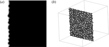
Interface deformation (isosurface
 $V_{f}=0.5$
) at the instant of the numerical transition from the compressible to the incompressible model for the 256 cross-section grid (
 ${\it\tau}\approx 5.78$
).

The density varies throughout the computational domain in the compressible model, whereas the variable-density incompressible model assumes that the density is constant in all computational cells except for cells where mixing occurs. Therefore, in the transition from compressible to incompressible, the density of the pure fluids and the density inside the mixing layer are recalculated. At the end of the compressible simulation, the incompressible densities
 $({\it\rho}_{1})_{I}$
and
 $({\it\rho}_{2})_{I}$
are computed by averaging the densities of cells where only pure fluid 1 or 2 is present. The averaged values allow the reconstruction of the incompressible mixing layer based on
 $V_{f}$
:
 $$\begin{eqnarray}({\it\rho}_{MIX})_{I}=V_{f}({\it\rho}_{1})_{I}+(1-V_{f})({\it\rho}_{2})_{I}.\end{eqnarray}$$
In the above formula, the densities are obtained from the averaging process and the
 $V_{f}$
distribution from the compressible solution. The density reconstruction is based on the volume fraction instead of the density field because in the compressible simulation the same volume fraction for given cells does not (necessarily) correspond to the same density values. Therefore, average densities for all the cells with
 $V_{f}=1$
and
 $V_{f}=0$
are calculated, and the density
 ${\it\rho}$
throughout the domain is recalculated according to the volume fraction distribution. In the numerical transition the momentum terms
 ${\it\rho}u$
,
 ${\it\rho}v$
and
 ${\it\rho}w$
are not modified. The pressure is initialised by a constant value, which is corrected by the incompressible solver at each time step, so as to satisfy the divergence-free constraint.
4. Numerical simulations
Unless otherwise specified, the results presented in this section refer to the finest grid. The simulations were carried out on Cranfield University’s high performance computing facility, Astral, using 64 processors. The approximate computational time for the compressible simulations was 90 days for
 ${\it\tau}=500$
. The corresponding time for the hybrid solver was 10 days for
 ${\it\tau}=1500$
. This clearly shows the computational advantage gained by the hybrid solver, which allows longer periods of mixing development to be computed in less computing time.
In order to allow the comparison of the results on different grid resolutions by taking into account the grid dependence of the initial perturbation, the time is non-dimensionalised by the minimum wavelength at the interface,
 ${\it\lambda}_{min}=16{\rm\Delta}x$
,
 $$\begin{eqnarray}{\it\tau}=t\frac{A_{t}^{+}{\rm\Delta}u}{{\it\lambda}_{min}}.\end{eqnarray}$$
The incompressible solver is initialised at
 $t_{NT}\approx 0.156$
s, which corresponds to non-dimensional times of approximately 5.78 and 11.56 for 256 and 512 resolutions respectively. The densities assigned to the incompressible fluids after the transition are
 $({\it\rho}_{1})_{I}=5.23$
and
 $({\it\rho}_{2})_{I}=1.82$
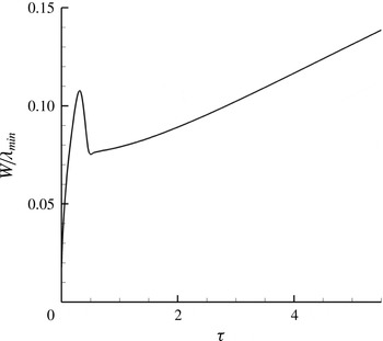
. The status of the interface at the end of the compressible part of the simulation is presented in figure 1. The linear growth of the mixing layer (figure 2) is dictated by the larger scales generated by the perturbed interface. An initial velocity is given to the gas interface so that the centre of the interface remains stationary after the passage of the shock wave. The initial growth of
 $W$
prior to the interaction of the shock wave with the interface is due to numerical diffusion of the interface (figure 2). This is followed by compression due to the interaction of the shock wave with the interface, hence the abrupt reduction in
 $W$
.
Growth of the mixing layer during the compressible stage for the 256 cross-section grid (
 $0<{\it\tau}<5.78$
). The rapid decay after the overshoot at
 ${\it\tau}\approx 0.3$
is due to compression of the initially diffused interface when the shock wave interacts with it.

4.1. Growth of the instability
The integral length of the mixing zone,
 $$\begin{eqnarray}W=\int \overline{V_{f}}(1-\overline{V_{f}})\,\text{d}x,\end{eqnarray}$$
where
 $\overline{V_{f}}$
is the volume fraction averaged over the
 $y$
and
 $z$
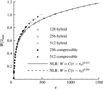
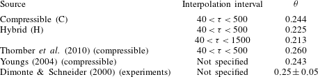
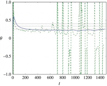
planes of the domain, is shown in figure 3 for both the compressible and the hybrid solutions. Furthermore, with reference to (2.3), the values of the growth exponent computed by the nonlinear regression (NLR) analysis are summarised and compared with published results in table 2.
Growth of the integral length of the mixing zone computed by the hybrid solver and interpolated using nonlinear regression analysis. The results of the compressible simulation from Thornber et al. (Reference Thornber, Drikakis, Youngs and Williams2010) are also shown.

Growth exponent values for various compressible and hybrid simulations, as well as experiments.
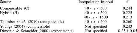
The growth exponent in the compressible simulation is found to be in good agreement with both the experiments of Dimonte & Schneider (Reference Dimonte and Schneider2000) and the numerical simulations of Thornber et al. (Reference Thornber, Drikakis, Youngs and Williams2010). Excellent agreement is also found with Youngs (Reference Youngs2004), where
 ${\it\theta}=0.243$
was obtained from a long-time compressible simulation; the difference between the simulation of Youngs (Reference Youngs2004) and our simulations is approximately
 $0.001$
. The hybrid simulation generally predicts a lower exponent independently of the time interval across which
 $W$
is interpolated. The value of
 ${\it\theta}$
obtained for
 $40<{\it\tau}<500$
slightly changes when the interpolation time window covers the entire simulated time, i.e.
 $40<{\it\tau}=1500$
. The differences between the present compressible simulation and the one by Thornber et al. (Reference Thornber, Drikakis, Youngs and Williams2010) are attributed to the different discretisation methods used, specifically the numerical dissipation embedded on the non-oscillatory schemes.
Further analysis on the estimation of
 ${\it\theta}$
, analogous to the methods applied by Dimonte et al. (Reference Dimonte, Youngs, Dimits, Weber, Marinak, Wunsch, Garasi, Robinson, Andrews, Ramaprabhu, Calder, Fryxell, Biello, Dursi, MacNeice, Olson, Ricker, Rosner, Timmes, Tufo, Young and Zingale2004) and Ristorcelli & Clark (Reference Ristorcelli and Clark2004) to estimate the growth rate coefficient for Rayleigh–Taylor mixing, is presented below. If we assume that the growth of the Richtmyer–Meshkov mixing layer is modelled by power-law growth with a virtual time offset
 $$\begin{eqnarray}W=A(t-t_{0})^{{\it\theta}},\end{eqnarray}$$
then we can derive the parameters
 $A$
,
 $t_{0}$
and
 ${\it\theta}$
from numerical data using the time derivatives of
 $W$
. If
 $t_{0}$
is assumed to be small, then we need only the first derivative
 $$\begin{eqnarray}{\it\theta}_{1}=\frac{t{\dot{W}}}{W},\end{eqnarray}$$
while if we allow for
 $t_{0}\neq 0$
, then
 $$\begin{eqnarray}{\it\theta}_{2}=\frac{1}{1-W\ddot{W}/{\dot{W}}^{2}}.\end{eqnarray}$$
In order to generate these estimates of
 ${\it\theta}$
, the first and possibly second derivatives of the layer thickness need to be found. Doing this by simple differencing of noisy data is known to be a numerically unstable procedure. In order to mitigate this numerical noise, we pass the layer width data through a Savitzky–Golay filter, with a weighting function applied to smooth the edges of the filter window, and hence reduce the effect of sudden changes as individual data points enter it. The results of the above analysis are shown in figure 4. The noisier method (
 ${\it\theta}_{2}$
) depends on second derivatives, so suffers from noise at late time. Overall, the above results seem to give pretty good evidence for convergence, though the way in which the first-order curve starts to wallow at late time (and the second-order version goes haywire) suggests that the dominant modes are starting to see the box size.


On comparing the hybrid solution with the various analytical theories, the results agree with Barenblatt’s suggestion for
 ${\it\theta}=2/3-{\it\nu}$
, where
 ${\it\nu}<1$
is a viscous correction. The hybrid and compressible simulations give
 ${\it\nu}\approx 0.45$
and
 ${\it\nu}\approx 0.42$
, which are within the range proposed by Barenblatt et al. (Reference Barenblatt, Looss and Joseph1983). The compressible simulations of Youngs (Reference Youngs2004) and Thornber et al. (Reference Thornber, Drikakis, Youngs and Williams2010) are also within this range, giving
 ${\it\nu}\approx 0.41$
and
 ${\it\nu}\approx 0.42$
respectively. The values obtained here are significantly lower than the range proposed by Zhou (Reference Zhou2001), which predicts an upper value of
 $2/3$
. However, the agreement between the numerical and the experimental results is good and confirms the (generally) accepted viscous correction theory of Barenblatt et al. (Reference Barenblatt, Looss and Joseph1983).
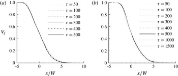
Profiles of the volume fraction, averaged on the
 $x$
planes, plotted against the direction of the shock propagation normalised by the integral length of the mixing layer at different (dimensionless) times for the fine grid. (a) Compressible; (b) hybrid.

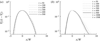
Profiles of
 $\overline{V_{f}}(1-\overline{V_{f}})$
, averaged on the
 $x$
planes, plotted against the direction of the shock propagation normalised by the integral length of the mixing layer at different (dimensionless) times for the fine grid. (a) Compressible; (b) hybrid.

Information about the self-similar growth of the mixing layer is obtained by plotting the plane-averaged profiles of the volume fraction at different instants in time (figure 5). In order to compare the solutions, the variable is normalised by the width of the mixing layer at the time instant considered. The profiles of figure 5 indicate that for both the compressible and hybrid solutions the evolution of the bulk of the mixing layer tends to become self-similar at
 ${\it\tau}\approx 250$
, whereas the two extremes of the mixing layer require more time to achieve this regime. The comparison is made clearer by plotting the quantity
 $\overline{V_{f}}(1-\overline{V_{f}})$
in figure 6. In the compressible simulations, the spikes do not become self-similar by the end of the simulated time (
 ${\it\tau}\approx 500$
). In the hybrid simulations, we found that the profiles start to develop in a self-similar manner after
 ${\it\tau}>500$
.
The differences in the extremities of the mixing layer are caused by density differences and, in turn, by the momentum of bubbles and spikes. This makes the profiles of the volume fraction asymmetric with respect to the centre of the mixing zone. The higher momentum of the spikes generates coherent vortex rings that travel away from the interface, which further break down and become part of the mixing layer only at later time in comparison with the bubbles. The evolution towards self-similarity as predicted by the hybrid simulation is found to be in good agreement with the compressible analysis of Thornber et al. (Reference Thornber, Drikakis, Youngs and Williams2010) which obtained self-similar evolution for the centre of the mixing layer at
 ${\it\tau}\approx 238$
. In Thornber et al. (Reference Thornber, Drikakis, Youngs and Williams2010), a value for bubbles and spikes was not predicted since the simulation ran up to
 ${\it\tau}=500$
and at that time it was found that although the profiles were tending towards collapsing on top of each other, self-similarity was still not yet clearly achieved. The above facts imply that a much finer grid resolution is necessary to correctly capture the extremities of the mixing layer since the fine structures in this region of the domain make the results extremely sensitive to the dissipative characteristics of the numerical scheme at high wavenumbers.
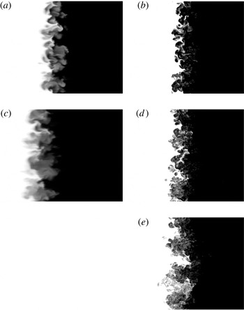
Visualisations of the evolution of the mixing layer are presented in figure 7, where the breakdown of the larger structures at late time and the turbulent development of the mixing layer are shown. It should be mentioned that the mixing fraction parameter after the transition remains the same by numerical construction, when using the volume fraction to initialise the density field. The differences in the volume fraction contours between compressible and hybrid simulations are attributed to the different inherent numerical dissipation associated with the incompressible and compressible ILES. It appears that the compressible solution is more dissipative than the incompressible one. This is similar to the single-mode case (Oggian et al. Reference Oggian, Drikakis, Youngs and Williams2014), where the incompressible solver predicted mushrooms with two roll-ups, whereas the compressible solver gave one roll-up. Although investigation of the properties of ILES models is beyond the scope of the present study, further research is required to analyse the dissipation and dispersion effects of different ILES models.
Two-dimensional visualisations of compressible (a,c) and hybrid (b,d,e)
 $V_{f}$
contour plots: (a,b)
 ${\it\tau}=200$
; (c,d)
 ${\it\tau}=500$
; (e)
 ${\it\tau}=1500$
. For
 ${\it\tau}=1500$
only hybrid visualisations are available. The plots are clipped to highlight the mixing layer.

Time evolution of the molecular mixing fraction,
 ${\it\Theta}$
, and the mixing parameter,
 ${\it\Xi}$
, for the 512 cross-section grid.

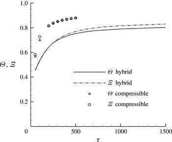
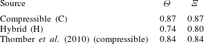
Figure 8 shows the evolution of the molecular mixing fraction,
 ${\it\Theta}$
, and the mixing parameter,
 ${\it\Xi}$
, defined as
 $$\begin{eqnarray}{\it\Theta}=\frac{\displaystyle \int \overline{V_{f}(1-V_{f})}\,\text{d}x}{\displaystyle \int \overline{V_{f}}(\overline{1-V_{f}})\,\text{d}x},\quad {\it\Xi}=\frac{\displaystyle \int \overline{\min (V_{f},1-V_{f})}\,\text{d}x}{\displaystyle \int \min (\overline{V_{f}},\overline{1-V_{f}})\,\text{d}x}.\end{eqnarray}$$
The
 ${\it\Theta}$
and
 ${\it\Xi}$
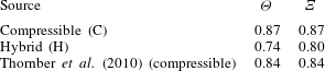
mixing parameters are measures of the total reaction rates for slow and fast reactions respectively. Both coefficients follow a similar trend but the compressible simulations give higher values. The curves do not reach a plateau for the simulation interval considered here but are characterised by a very low positive slope which decreases with time. Table 3 summarises the asymptotic values and compares them with the results of Thornber et al. (Reference Thornber, Drikakis, Youngs and Williams2010). The hybrid solution predicts less mixing, and lower
 ${\it\Theta}$
and
 ${\it\Xi}$
than the compressible solution, which is also evident from the volume fraction plots in figure 7. The
 ${\it\Theta}$
and
 ${\it\Xi}$
as obtained from the present compressible simulations are very similar to the compressible results of Thornber et al. (Reference Thornber, Drikakis, Youngs and Williams2010) despite the fact that different numerical methods were used in the two compressible simulations. The above results give confidence regarding the compressible ILES models but also suggest that further investigation and comparison between incompressible and compressible ILES are required.
Values of the mixing parameters for compressible and hybrid simulations compared with the compressible simulation from Thornber et al. (Reference Thornber, Drikakis, Youngs and Williams2010).
4.2. Turbulent kinetic energy (TKE)
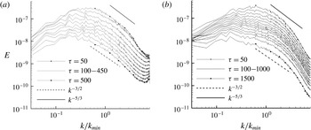
The TKE spectra for the hybrid and compressible simulations at various time instants are shown in figure 9. The spectra have been obtained by an averaging process over 10 slices of the domain along the
 $x$
direction, which is the direction of the shock propagation. These slices are selected to be at the centre of the mixing layer.
Compressible and hybrid spectra of the radial turbulent kinetic energy averaged on the
 $y$
and
 $z$
planes in the bulk of the mixing layer for the 512 cross-section grid and the
 $k^{-3/2}$
guideline analytically predicted by Zhou (Reference Zhou2001). (a) Compressible solution; spectra for
 ${\it\tau}=50$
, 100, 150, 200, 250, 300, 350, 400, 450 and 500. (b) Hybrid solution; spectra for
 ${\it\tau}=50$
, 100, 150, 200, 250, 300, 350, 400, 450, 500, 600, 700, 800, 1000 and 1500.

Previous studies (Zhou Reference Zhou2001; Thornber et al.
Reference Thornber, Drikakis, Youngs and Williams2010) have shown that the spectrum of the narrowband layer prior to reshock takes a
 $k^{-3/2}$
form. Immediately following reshock (where the shock has moved fully clear of the layer) there is a
 $k^{-5/3}$
range present in the spectrum; however, at the latest time where the flow tends towards a self-similar solution the spectrum returns to a
 $k^{-3/2}$
form but with more energy at lower wavenumbers than in the pre-reshock case. As the growth rate of the mixing layer is essentially the integral of the kinetic energy spectrum, the slight increase of the growth exponent is most likely due to this increase in low-wavenumber energy.
The above ranges are also observed in the present spectra; however, comparing with the results of Thornber et al. (Reference Thornber, Drikakis, Youngs and Williams2010) the agreement is less clear in the present compressible simulations due to the coarser resolution,
 $512^{2}$
cross-section here versus
 $2048^{2}$
in Thornber et al. (Reference Thornber, Drikakis, Youngs and Williams2010). The
 $k^{-5/3}$
region in the hybrid simulations is also limited to a shorter range of wavenumbers compared with the compressible results. These discrepancies are attributed to the scaling of the initial perturbation and the discretisation methods. The results clearly show that the numerical dissipation has important effects on the flow physics, and considering that most practical simulations are under-resolved with respect to the grid, this issue requires more investigation. Bearing the aforementioned uncertainties in mind, the results further show that the energy peak progressively moves from an initial
 $k/k_{min}\approx 0.6$
at
 ${\it\tau}=40$
to
 $k/k_{min}\approx 0.1$
at
 ${\it\tau}=1500$
. At high wavenumbers (
 $k/k_{min}>3$
), the rate of TKE decay increases, but at the very end of the spectrum,
 $k/k_{min}\approx 8$
, a slight turn-up of the energy is observed. This part of the spectrum still represents the unknown since there is no theory that describes the dissipative characteristics of shock-induced turbulent mixing. The turn-up in the dissipation range of the compressible spectrum appears to be more evident. The results obtained from both simulation approaches indicate that at the end of the simulation there is no evidence of memory loss of the initial shock and the mixing still behaves in an inhomogeneous and anisotropic manner.
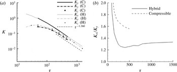
Evolution in time of the turbulent kinetic energy components and of the ratio
 $K_{x}/K_{y}$
for the 512 cross-section grid, for both the compressible and hybrid simulations: (a) TKE components; (b)
 $K_{x}/K_{y}$
ratio.

The evolution of the TKE components defined by
 $$\begin{eqnarray}K_{x}=\frac{1}{2}\int {\it\rho}(u-\overline{u})^{2}\,\text{d}V,\quad K_{y}=\frac{1}{2}\int {\it\rho}v^{2}\,\text{d}V,\end{eqnarray}$$
where
 $$\begin{eqnarray}\overline{u}=\frac{\displaystyle \int _{y,z}{\it\rho}u\,\text{d}S}{\displaystyle \int _{y,z}{\it\rho}\,\text{d}S},\end{eqnarray}$$
is shown in figure 10. There is good agreement between the compressible and hybrid simulations. At early times,
 $K_{x}$
is an order of magnitude larger than
 $K_{y}$
and
 $K_{z}$
. As time passes, the behaviours of the longitudinal and radial components follow different trends. The former constantly decreases, whereas the latter presents an initial growth until
 ${\it\tau}\approx 40$
and then it successively diminishes until the end of the simulation.
As has been discussed in Thornber et al. (Reference Thornber, Drikakis, Youngs and Williams2010), given that the width of the mixing layer scales with
 $t^{{\it\theta}}$
, the empirical relation
 ${\it\epsilon}\propto u^{3}/W$
can be used to check the dissipation rate of kinetic energy. From dimensional analysis
 $\text{d}K/\text{d}t\propto K^{3/2}/t^{{\it\theta}}$
, where
 $K$
is the turbulent kinetic energy per unit mass, with a solution of the form
 $K\propto t^{2{\it\theta}-2}$
. This is the decay rate of mean kinetic energy across the mixing layer. The decay of the total fluctuating kinetic energy is proportional to the width of the mixing layer multiplied by the mean kinetic energy, i.e.
 $WK\propto t^{{\it\theta}}t^{2{\it\theta}-2}\propto t^{3{\it\theta}-2}$
. This result can also be gained by assuming that the mean velocity in the mixing layer is proportional to the growth of the mixing layer itself, giving
 $\sqrt{K}\propto \text{d}W/\text{d}t\propto t^{{\it\theta}-1}$
, i.e.
 $WK\propto t^{3{\it\theta}-2}$
. Considering that the hybrid solver returned a growth coefficient of
 ${\it\theta}=0.213$
, the TKE is supposed to scale with
 $t^{-1.36}$
. From figure 10(a), it is clear that the decay of
 $K$
is consistent with the prediction. As a consequence of the evolution of the TKE in time, the ratio of
 $K_{x}$
to the radial components decreases very quickly, until it reaches a minimum of 1.24 at
 ${\it\tau}\approx 400$
, followed by a slow increase. For
 $800<{\it\tau}<1500$
, the ratio
 $K_{x}$
/
 $K_{y}$
is included in the range
 $1.315\pm 0.015$
with the tendency to increase.
The analysis of the TKE components is also consistent with the TKE spectra. Even though the trend of these quantities results in a constant and basically equal decay at the end of the simulation, e.g. at
 ${\it\tau}\approx 250$
the rate of decay for all components becomes almost identical, there is no sign of loss of anisotropy in the flow field as the
 $x$
component of the TKE is higher than the radial contributions; this conclusion also agrees with Thornber et al. (Reference Thornber, Drikakis, Youngs and Williams2010). The ratio
 $K_{x}/K_{y}$
found in this study seemed to stabilise around a value of
 $1.25\pm 0.02$
at
 ${\it\tau}>50$
. In comparison with the compressible simulations, the hybrid approach gives a lower anisotropy at late times.
5. Conclusions
A computational approach for studying the late-time development of the Richtmyer–Meshkov instability was presented. The method utilises a compressible flow model at early times and an incompressible one at later times. The proposed approach enables longer times of the mixing development to be simulated in shorter computational time. The results were found to be in good agreement with previous compressible simulations, theory and experiments.
The simulations indicated that the spikes and bubbles start to converge towards self-similar behaviour at different time instants, approximately
 ${\it\tau}=600$
for spikes and
 ${\it\tau}=250$
for bubbles. The mixing parameters of the present compressible simulations were found to be in good agreement with the compressible flow results of Thornber et al. (Reference Thornber, Drikakis, Youngs and Williams2010). The hybrid solution gives less mixing than the compressible solution. Furthermore, the
 $k^{-3/2}$
region of the TKE spectra of the hybrid simulations is limited to a shorter range of wavenumbers compared with the compressible simulations. The discrepancies between different ILES models and simulations are attributed to the scaling of the initial perturbation and the discretisation methods. The numerical dissipation has significant effects on the flow physics, and this issue deserves further investigation. Contrary to what is assumed in Zhou (Reference Zhou2001), the TKE spectra indicated an anisotropic evolution even at late times. In fact, although the averaged TKE components were found to decay at the same rate of
 $t^{-1.36}$
, at late time the
 $x$
component exhibited an absolute value approximately 1.31 times higher than the same parameter along the
 $y$
and
 $z$
directions.
Although the results of the present study are promising with respect to the use of hybrid compressible–incompressible methods for simulating late-time RMI mixing, they also suggest that further research is required to elucidate the physics of the RMI (anisotropy and self-similarity) and the effects of numerical methods, ILES in particular, on the simulation results. The results suggest that although the time window of the simulations has been extended thanks to the hybrid method, the flow has not yet become fully self-similar. Olson & Greenough (Reference Olson and Greenough2014) suggested that the number of grid points needed for a direct numerical simulation of the RMI is approximately
 $4\times 10^{12}$
, which exceeds the current capabilities of supercomputing resources. For an RM calculation with fixed small scales computed with an explicit hydrodynamics scheme, the computational cost to get to width
 $W$
will be
 $\propto W^{3}W^{1/{\it\theta}}$
, where the first term is the number of cells required to resolve the mixing layer and the second term is the number of time steps required. Therefore, the computational time cost expands roughly as the dynamic range
 $(W/{\rm\Delta}x)^{7}$
. The easiest factor to address is the
 $W^{1/{\it\theta}}$
, which an implicit calculation should be able to change to
 $\propto W$
or
 $\propto W$
log
 $W$
. Beyond that, it may be possible to gain extra factors, e.g. by de-refining fine scales at late time. In summary, even two orders of magnitude higher resolution than the one employed here would seem to require exclusive access to the largest high performance power computing facilities currently available. Therefore, future research should justify what resolution is needed to get reliable results (for relevant parameters, in relevant conditions) from an ILES calculation with the particular numerical methods being used. Finally, part of our future research will also be to use the hybrid method to examine the effects of different initial conditions on late-time mixing.
Acknowledgements
D.D. wishes to express his gratitude and appreciation to AWE for their financial support through the William Penney Fellowship award. AWE’s financial support with respect to TO’s PhD Case Award is also greatly acknowledged. The manuscript contains material © British Crown Owned Copyright 2015/AWE, reproduced with permission.