1. Introduction
Scramjets, as the most promising propulsion system for air-breathing hypersonic vehicles, face critical challenges in achieving rapid ignition and stable pilot flames under high-speed conditions (Curran Reference Curran2001; Li et al. Reference Li, Cai, Ji, Wang and Sun2025). Sufficient fuel–air mixing is a prerequisite for efficient combustion. However, the compact geometry of cavity flameholders and the exceedingly short fuel residence time inherently limit the mixing efficiency (Choubey et al. Reference Choubey, Devarajan, Huang, Mehar, Tiwari and Pandey2019; Oamjee & Sadanandan Reference Oamjee and Sadanandan2020; Nair, Suryan & Narayanan Reference Nair, Suryan and Narayanan2024). For mixing enhancement in the cavity flameholders, various flow control methods have been proposed, including passive methods that manipulate the external flow fields via intrusive geometries (Sathiyamoorthy et al. Reference Sathiyamoorthy, Danish, Iyengar, Manjunath, Muruganandam and Chakravarthy2020; Abdelmwgoud & Mohany Reference Abdelmwgoud and Mohany2021), and active methods such as plasma actuation (Houpt et al. Reference Houpt, Leonov, Ombrello, Carter and Leiweke2019; Wang et al. Reference Wang, Chen, Feng, Ding, Huang and Tian2024) and transverse jet injection (Song et al. Reference Song, Wang, Sun, Cai, Liu and Yu2019; Choubey et al. Reference Choubey, Yadav, Devarajan and Huang2021). Compared with the passive methods, active flow control (AFC) offers greater flexibility and incurs no drag penalty in off-design conditions (Cattafesta & Sheplak Reference Cattafesta and Sheplak2011). The core of AFC lies in its control strategy. Due to the significant complexity involved in deriving an optimal closed-loop control strategy for unsteady flows (Duriez, Brunton & Noack Reference Duriez, Brunton and Noack2017), the actuators in AFC are mostly operated in open-loop (OL) mode with prescribed actuation parameters such as the frequency and amplitude (Kong et al. Reference Kong, Wang, Zong, Wu, Liang, Tang and Qu2025a , Reference Kong, Zong, Wang, Wu, Su, Wei, Jia and Tangb ).
1.1. The OL control of cavity flows
The effectiveness of OL control in supersonic cavity flows depends strongly on the matching between the actuation parameters (e.g. location, frequency, amplitude) and the cavity geometric configurations (Gruber et al. Reference Gruber, Baurle, Mathur and Hsu2001). So far, significant efforts have been made to identify the optimal parameter combination that leads to the most mixing enhancement or noise suppression. In Yugulis et al. (Reference Yugulis, Hansford, Gregory and Samimy2014) and Webb & Samimy (Reference Webb and Samimy2017), by positioning arc plasma actuators at 1 mm upstream of the cavity leading edge, dominant Rossiter-mode tones and broadband pressure oscillations were suppressed noticeably in high-subsonic (Mach 0.6) and supersonic (Mach 2.24) flows, respectively. Inspired by these findings, Kong et al. (Reference Kong, Wu, Zong and Guo2022) deployed a spanwise array of pulsed-arc plasma actuator (PAPA) in front of the cavity leading edge, and the Kelvin–Helmholtz (K–H) instabilities in Mach 2 cavity flow were excited by plasma-induced thermal perturbations, resulting in a large-scale wavy motion of the cavity shear layer. Subsequent work by Wang et al. (Reference Wang, Chen, Feng, Ding, Huang and Tian2024) proved that the fluctuation intensity of the shear layer is positively correlated with the actuation frequency. In Oka et al. (Reference Oka, Ozawa, Handa and Nonomura2024), high-frequency flapping and non-flapping jets were both adopted to modulate the pressure fluctuations in cavity flow, and by wisely selecting the actuation location and frequency, the shear layer fluctuations can be amplified sixfold. Inspiring results were also demonstrated by Kong et al. (Reference Kong, Zong, Wang, Wu, Su, Wei, Jia and Tang2025b), where a travelling-wave actuation implemented via a PAPA matrix achieved one order of magnitude increase in the spectrum peak of shear layer velocity fluctuation, when compared with the baseline. Kong et al. (Reference Kong, Wang, Zong, Wu, Liang, Tang and Qu2025a) further tested the impact of the back-wall inclination angle. Compared with their previous study (Kong et al. Reference Kong, Zong, Wang, Wu, Su, Wei, Jia and Tang2025b ), although different actuators were used (plasma synthetic jets), similar trends of decreasing control efficacy with increasing back-wall inclination angle were concluded, largely due to the intrinsically strong pressure feedback at high back-wall angles.
1.2. Deep reinforcement learning control in numerical simulations
Over the past decade, machine learning methods, including linear genetic programming and deep reinforcement learning (DRL), have emerged as powerful tools for realising closed-loop flow control in both numerical simulations and experiments (Brunton, Noack & Koumoutsakos Reference Brunton, Noack and Koumoutsakos2020). A major merit of machine learning control is the complete elimination of the modelling process. Taking DRL as an example, the control policy is trained by analysing the sensor feedback from trial-and-error actuation commands. Since extensive information needs to be extracted from the flow, and the neural network has to be computed after each control step, practical implementations of DRL are much more challenging than traditional OL control (Vignon, Rabault & Vinuesa Reference Vignon, Rabault and Vinuesa2023). Consequently, the majority of the early DRL flow control studies were performed in low-Reynolds-number simulation environments, e.g. the vortex shedding suppression in cylinder wake flow at
 $\textit{Re} = 100{-}1000$
(Rabault et al. Reference Rabault, Kuchta, Jensen, Réglade and Cerardi2019; Ren, Rabault & Tang Reference Ren, Rabault and Tang2021). Recent years have witnessed DRL’s effective applications in higher-
 $\textit{Re}$
scenarios. Sonoda et al. (Reference Sonoda, Liu, Itoh and Hasegawa2023) utilised the deep deterministic policy gradient (DDPG) algorithm with a nonlinear activation function to generate an optimal blowing/suction strategy, achieving a 31 % drag reduction in a full-size channel flow. Guastoni et al. (Reference Guastoni, Rabault, Schlatter, Azizpour and Vinuesa2023) proposed a computationally efficient multi-agent DRL framework for turbulent drag reduction in channel flow, and prominent drag reduction magnitudes of 43 % and 30 % were reported in a minimal channel and a larger channel at
 $\textit{Re}_\tau = 180$
through the DDPG algorithm. Font et al. (Reference Font, Alcántara-Ávila, Rabault, Vinuesa and Lehmkuhl2025) demonstrated that multi-agent DRL combined with the proximal policy optimisation algorithm can outperform periodic jets by 61 % in suppressing turbulent separation bubbles, autonomously discovering a multi-frequency streamwise vortex control strategy. Actor–critic frameworks based on stochastic policies, which avoid reliance on experience replay buffers, are well suited for online learning at high Reynolds numbers. Recently, Chen, Ballini & Micheletti (Reference Chen, Ballini and Micheletti2025) implemented such a framework, achieving drag reduction and lift oscillation suppression in a circular cylinder flow at
 $\textit{Re} = 274\,000$
. Despite these successes, the substantial computation time required to collect sufficient training data in high-Reynolds-number numerical flow environments can be overwhelming for the AFC community.
1.3. The DRL control in experiments
In experimental DRL flow control, the curse of the Reynolds number no longer exists as long as we have suitable facilities. However, the true challenge comes from the critical time requirements imposed on sensor acquisition, control law computation and actuator commanding. Specifically, the cumulative latency from these processes has to be less than the characteristic time scale of the flow (Zong et al. Reference Zong, Wu, Li, Su and Liang2025). Otherwise, the dynamics of the flow is missing, which might lead to a degradation of the DRL control performance (Rabault & Kuhnle Reference Rabault and Kuhnle2019). Pioneering experiments were conducted in Fan et al. (Reference Fan, Yang, Wang, Triantafyllou and Karniadakis2020), which demonstrated the effectiveness of DRL for bluff-body flow control in a low-speed water tunnel. Since the flow velocity is only 0.2 m s−1, they implemented a 10 Hz control loop frequency. Dong et al. (Reference Dong, Wang, Lin, Wang and Hu2024) developed an interactive platform integrating DRL with wind tunnel testing, using a universal adapter to facilitate communications between the sensors and DRL libraries. However, their action update cycle was 6–10 s (corresponding to frequency 0.1–0.17 Hz), substantially lower than the vortex shedding frequency (6–20 Hz) of the flow around their square cylinder test case. Additionally, Shimomura et al. (Reference Shimomura, Sekimoto, Oyama, Fujii and Nishida2020) and Amico, Cafiero & Iuso (Reference Amico, Cafiero and Iuso2022) conducted experimental DRL of aerofoil flows and three-dimensional bluff-body wakes, respectively. Due to the usage of CPU as the core controller, a significant communication delay of the order of 1–10
 $\textrm{ms}$
exists between the data acquisition devices and the control unit, which limits the interaction frequency between the controller and the flow field below 100 Hz. This CPU-based DRL control architecture might be able to catch up with the flow dynamics at 1–10 m s−1, but definitely not enough to perform a real-time closed-loop control of the high-speed flow of the order of 100 m s−1, necessitating a breakthrough in hardware architecture. To deal with the above challenge, a novel field-programmable gate array (FPGA) based DRL framework (FeDRL) was developed by Zong et al. (Reference Zong, Wu, Li, Su and Liang2025). Since real-time high-frequency control (deployed on the FPGA) and neural network training (run on CPU) are effectively split, a control interaction frequency 1–10 kHz can be achieved, almost a two-order speed-up over CPU-based DRL control systems. The effectiveness of this framework has been validated in several scenarios, such as the flow separation control behind a backward-facing step flow (
 $\textit{Re}=2.9\times 10^4$
) (Xiang et al. Reference Xiang, Zong, Wu, Li and Liang2024), and the mixing enhancement in a supersonic backward-facing step flow at Mach 2.0 (
 $\textit{Re}=2.9\times 10^6$
) (Zong et al. Reference Zong, Wu, Li, Su and Liang2025). Compared with numerical DRL, the most attractive feature of FeDRL probably goes to the high efficiency, requiring only tens of seconds of wind tunnel running time to derive a satisfactory closed-loop control law.
1.4. Initiative and objective of the present study
Based on the above review, it is clear that DRL, when applied to closed-loop flow control, can help us to release the potential of actuators and discover novel control strategies with enhanced benefits. However, so far, such a powerful tool has not set foot in the supersonic cavity flow. This paper fills this blank by performing the first DRL control of a supersonic cavity flow in a wind tunnel environment. Three innovations should be mentioned. First, unlike previous studies where only one column of actuators was used (Zong & Kotsonis Reference Zong and Kotsonis2019; Tang et al. Reference Tang, Wu, Zong, Luo, Yang and Guo2022), a 4
 $\times$
5 PAPA matrix with independently controllable columns and cross-talk-free discharge circuits is designed, enabling instant adjustment of the actuator formation and location. In particular, with this PAPA matrix, we are able to operate the actuator in diverse modes, such as the synchronous fixed-formation (FF) mode, and the asynchronous variable-formation (VF) mode. Second, the optimal control strategy that links the instantaneous actuator formation with the flow state observation is optimised by a 16-output deep Q-network (DQN), based on the feedback signal measured by a specially designed supersonic hot wire. Third, the impacts of the cavity back-wall inclination angle on the DRL effectiveness are investigated, providing guidance for the practical design of the AFC system in cavity flameholders.
The paper is structured as follows. Section 2 first describes the experimental set-up, including the cavity flow model, actuator system and DRL control framework. Then, in § 3, the temporal response of cavity flow to plasma actuation is visualised with high-speed schlieren imaging, and the performances of DRL under different operation modes are examined in detail. Finally, the closed-loop control mechanisms are interpreted in § 4, and the major findings are summarised in § 5.
2. Experimental set-up
2.1. Cavity flow model
Experiments are conducted in a supersonic wind tunnel at the National Key Lab of Aerospace Power System and Plasma Technology. This wind tunnel is a suction-type transient wind tunnel driven by the pressure difference between the ambient atmosphere and a vacuum chamber. Interchangeable nozzles are configured to realise different Mach numbers. At Mach 2 (freestream velocity
 $U_\infty = 510$
m s−1), the total operation time of the wind tunnel is approximately 12 s. However, to get rid of the initial transient and ensure a stable inflow condition, DRL control is conducted only in the last 10 s. Detailed inflow and geometric parameters are documented in our previous study (Kong et al. Reference Kong, Wang, Zong, Wu, Liang, Tang and Qu2025a
), thus will not be repeated for brevity. As illustrated in figure 1, the cavity is embedded in a flat-plate model, featuring length (
 $L$
), depth (
 $D$
) and width (
 $W$
) measurements 50, 10 and 80 mm, respectively. Three interchangeable trailing-edge wedges with inclination angles
 $\theta = 30^\circ$
, 45
 $^\circ$
, 90
 $^\circ$
are designed to modify the cavity back-wall geometry. The distance from the cavity to the leading edge of the flat plate is
 $L_0 = 190$
mm. Using
 $L_0$
and
 $U_\infty$
as the reference length and velocity scales, the Reynolds number is calculated as
 $2\times 10^6$
.
(a) Axonometric view of the cavity model. (b) Cross-sectional view of the cavity model in the
 $xy$
-plane. (c) Cross-sectional view of the PAPA column.

A custom-designed strut (diameter 5 mm), made of stainless steel and featuring a wedge-shaped leading edge, supports the hot-wire probe with minimal flow disturbance. The tungsten hot-wire sensor has wire diameter 6.5
 $\mathrm{\unicode{x03BC}m}$
and wire length 2.4 mm, providing a maximum frequency response exceeding 10 kHz (ChangZhou Turbulence Technology, WHF-01). A coordinate system is established at the middle point of the cavity leading edge, with the
 $x$
-,
 $y$
- and
 $z$
-axes along the streamwise, wall-normal and spanwise directions, respectively. The wire is placed at a streamwise location corresponding to two-thirds of the cavity length, with approximate coordinates
 $(x,y,z)=(34,0,0)$
mm. A constant-temperature anemometer (Hanghua Technology, CTA-4) is used to drive the hot wire. The overheat ratio is set as 2.5 under cold flow, corresponding to operation temperature 410 K.
As described by the King’s law (King Reference King1914), the output voltage of the hot wire (denoted
 $E$
) can be written as
 \begin{equation} E^2 = (T_w - T_{\!f})(A + B\,\textit{Re}_w^n), \end{equation}
where
 $T_w$
and
 $T_{\!f}$
are the wire temperature and the fluid temperature, respectively,
 $\textit{Re}_w$
is the wire-diameter-based Reynolds number, taking the local fluid velocity and density as the reference scales, and
 $A$
and
 $B$
are constants related to the wire properties. As a result, in compressible flows, a variation in any of the three flow quantities (temperature, density and velocity) can cause a change in the hot-wire voltage. This implies that obtaining a unique ‘velocity–voltage’ calibration curve is impossible for the present experiment. Therefore, the raw voltage of the hot-wire sensor is directly used for subsequent analyses.
2.2. Plasma actuator
Figure 1 depicts the flush-mounted ceramic block containing a 4
 $\times$
5 actuator matrix. The four PAPA columns, oriented along the spanwise direction, are designated as
 $C_1$
–
 $C_4$
from downstream to upstream;
 $C_1$
is positioned 7 mm upstream of the cavity leading edge, and the streamwise spacing (
 $L_x$
) between adjacent PAPA columns is 14 mm (see figure 1
b). As shown in figure 1(c), each PAPA column is comprised of four U-shaped copper bars (cross-section size 2
 $\times$
2 mm) and two copper needles (diameter 1 mm), forming five arc discharge channels with air gap 1 mm (
 $L_z$
). The two copper needles, serving as the anode and cathode, respectively, are inserted into the thick high-voltage wires beneath them for the purpose of external electrical connection. As a result of the above design, each PAPA column operates as an independently controllable actuator unit.
The discharge circuit used to power the actuator matrix.

A sequential discharge system, adapted from Zong & Kotsonis (Reference Zong and Kotsonis2018), powers the actuator matrix. As shown in figure 2, each PAPA is driven by a stand-alone discharge unit consisting of a high-voltage trigger circuit and a capacitive discharge circuit. Four capacitors (
 $C_0$
, capacitance 0.1
 $\unicode{x03BC}$
F) are configured to store the discharge energy and are connected in parallel to a DC power supply (output voltage
 $U_0 = 800$
V). Between each capacitor and the DC power supply, a resistor (
 $R_1$
, resistance
 $200\ \Omega$
) is added to limit the charge current. Based on the principle of resistor–capacitor circuit, the charging time constant is computed as
 $\tau _c=R_1\times C_0=20\ {\rm\unicode{x03BC}\textrm{s}}$
. Theoretically, five times
 $\tau _c$
(namely 100
 $\unicode{x03BC}\textrm{s}$
) is required to fully charge the capacitor voltage to the output voltage of the DC power supply. Therefore, to ensure that the capacitor energy can always be restored during repetitive pulsed-arc discharge, the maximum operation frequency of the circuit should be no more than 10 kHz. In the present study, the upper limit of the discharge frequency is set as 5 kHz, and the capacitor energy (
 $E_c$
) deposited into the flow per shot is
 $E_c = 0.5\,C_1\,U^2_0=32$
mJ.
Taking the first PAPA column as an example, the workflow in one discharge period can be described as follows. First, an 8 kV trigger pulse is generated by a high-voltage pulse generator to ionise the electrode gaps, establishing a serially connected spark channel between the anode and cathode. Subsequently, the energy stored in the capacitor is rapidly released into the arc plasma, which imposes disturbances to the flow by thermal heating. To protect the high-voltage pulse generator from short circuit, a safeguard resistor (
 $R_2 = 10\ \text{k}\Omega$
) is inserted into the trigger circuit. Additionally, two high-voltage diodes (
 $D_1$
and
 $D_2$
) are used to prevent the possible current crosstalk between the DC power supply and the high-voltage trigger power supply. Based on the above description, it is clear that the discharge timing of each actuator column is determined purely by its own trigger pulse. Thus by selectively switching on the plasma actuators in different columns, a real-time dynamic switching of the actuator formation can be realised in closed-loop control. Denoting the status of each actuator column (switch-off/switch-on) as a logic number (0/1), the formation of the four-column actuator array can be encoded into a four-bit binary number (
 $FC$
), referred to as the formation code hereinafter. In total, we have 16 possible actions (denoted as
 $a_t$
), with
 $FC = 0000$
and
 $FC = 1111$
representing an all-on and an all-off formation, respectively.
2.3. The DRL control framework
Our control objective is to find an optimal control strategy that maximises the mixing in the supersonic cavity shear layer by dynamically selecting the most appropriate actuator formation code according to the instantaneous flow states measured by the hot wire. For this purpose, the original FPGA-based DRL control architecture proposed by Zong et al. (Reference Zong, Wu, Li, Su and Liang2025), which can only deal with simple logic control, is updated to incorporate a maximum of 16 actions. As illustrated in figure 3, the framework employs a DQN architecture with a real-time control loop (5 kHz) and a VF training loop running on the FPGA and the CPU, respectively. Necessary data including the network coefficients and control experiences are exchanged between the two loops via a direct memory access mechanism, which enables concurrent execution and training of the neural network control law. The communication between the FPGA program in the controller side and the Python program in the host side is facilitated through LabVIEW’s NI-FPGA module. Real-time performance is ensured by directly hooking the analogue-to-digital converter (ADC) and the digital-to-analogue converter (DAC) to the FPGA I/O ports.
Experimental closed-loop control framework based on FPGA and RBF network. Technical Data Management Streaming (TDMS ) is a file format for storing and retrieving engineering test data.

Since only one hot-wire sensor is configured, to provide more information about the flow, not only the current signal but also its historical signals are incorporated into the state vector (denoted as
 $\boldsymbol{x_t}$
), as follows:
 \begin{equation} \boldsymbol{x}_t=\left [s(t),s(t-\tau ),\ldots ,s(t-(l-1)\tau )\right ]\in {\rm Re} ^l. \end{equation}
In this equation,
 $\tau$
denotes the sample period, set as 20
 $\unicode{x03BC}$
s in this study,
 $l$
is the state length, determining how long the signal history is considered, and
 $s(t)$
is the dimensionless hot-wire voltage normalised using the relation
 \begin{equation} s(t)=\frac {u(t)-\bar {u}_{BL}}{\sigma _{u,BL}}, \end{equation}
where
 $\bar {u}_{BL}$
and
 $\sigma _{u,BL}$
denote the mean and standard deviation of the raw hot-wire voltage (
 $u(t)$
) under the baseline condition, respectively. As a result,
 $s(t)$
follows approximately a Gaussian distribution, varying within a typical range [
 $-3, 3$
]. For brevity of notation, we will use
 $s_t$
and
 $s_{t-l}$
to denote
 $s(t)$
and
 $s(t-(l-1)\tau )$
, respectively.
The state vector
 $\boldsymbol{x_t}$
is fed into a radial basis function (RBF) network for Q-value computation:
 \begin{equation} Q_{\boldsymbol{x}_t,a_t}=\sum _{i=1}^{m}W_{\!j,i}\exp(-h_i\,\|\boldsymbol{x}_t-\boldsymbol{c}_i\|^2)+B_{\!j}. \end{equation}
Here,
 $\boldsymbol{c}_i$
and
 $h_i$
denote the centre and width of the ith Gaussian kernel (
 $i=1, 2,\ldots , m$
), respectively;
 $W_{\!j,i}$
and
 $B_{\!j}$
represent the weights and bias of the output layer for the
 $j$
th action (
 $j=0, 1,\ldots , N$
), respectively;
 $m$
is the number of hidden neurons, and
 $N$
is the output dimension, namely the number of actions.
Based on the Q-values predicated by the RBF network, the action can be selected using an
 $\varepsilon$
-greedy policy:
 \begin{equation} \pi (\boldsymbol{x}_t,{a_t})=\begin{cases} 1-\varepsilon & \mathrm{if}\quad a_t=\mathrm{argmax}\{Q(\boldsymbol{x}_t,a_t)\}, \\ \displaystyle \frac {\varepsilon }{N-1} & \mathrm{otherwise}, \end{cases} \end{equation}
where
 $\varepsilon$
is the exploration probability, and
 $\pi$
is the policy function, namely the probability of selecting
 $a_t$
at a given state
 $s_t$
.
For efficient and stable learning, a proper instantaneous reward
 $r_t$
has to be defined. Considering that our prime objective is to enhance the mixing,
 $r_t$
is formulated by subtracting 1 from the root mean square of the dimensionless voltage signal over the next 10 steps:
 \begin{equation} r_t=\sqrt {\frac {1}{m}\sum _{i=1}^{m}({s}_{t+i})^2}-1. \end{equation}
Mathematically, it can be shown that the expectation of
 $r_t$
under the baseline condition is zero. Thus positive values of
 $r_t$
correspond to increased shear layer velocity fluctuations with respect to the baseline, while negative rewards correspond to decreased fluctuations.
Sketches of (a) the closed-loop DRL control process and (b) the timings of key steps in a control period. TTL for level signals and TCP/IP for internet communication protocols.

Based on the experiences collected by the controller, namely
 $(\boldsymbol{x}_t,a_t,r_t,\boldsymbol{x}_{t+1})$
, the network parameters including
 $\boldsymbol{c}_i$
,
 $h_i$
,
 $W_{\!j,i}$
and
 $B_{\!j}$
can be updated using the loss function
 \begin{equation} L=\mathbb{E}\Big [\Big (r_t+\gamma \times\max_{a_{t+1}}{\boldsymbol{Q}_{\textit{target}}}(\boldsymbol{x}_{t+1},a_{t+1})-{\boldsymbol{Q}}(\boldsymbol{x}_t,a_t)\Big )^2\Big ]. \end{equation}
Here,
 $\gamma$
is the reward discount factor, and
 $\boldsymbol{Q}_{\textit{target}}$
denotes the target Q-network, a key component of the classic DQN algorithm (Mnih et al. Reference Mnih2015). In offline reinforcement learning, the target network is essential for learning stability. It provides temporally consistent target values by periodically copying parameters from the online network, thereby reducing the correlation between the current Q-value estimates and their targets, and mitigating the risk of divergence when learning from a fixed dataset (Kumar et al. Reference Kumar, Zhou, Tucker and Levine2020; Levine et al. Reference Levine, Kumar, Tucker and Fu2020). It was introduced to mitigate the Q-value overestimation issue caused by bootstrapping. The variable
 $a_{t+1}$
denotes the action proposed by this target Q-network at the next time step, which is not necessarily equal to the actual next action
 $a_{t+1}$
. To ensure learning stability within the DQN framework, the original Q-network is updated after each training iteration, while the target Q-network is copied from the original Q-network once every five training iterations. The updated network parameters in Python are eventually relayed back to the FPGA controller via a first in, first out (FIFO) sequence.
The above-mentioned closed-loop control process is summarised in figure 4(a). First, at each control step, the instantaneous state of flow is sensed by a hot wire, and the output voltage is acquired as
 $u(t)$
. Then
 $u(t)$
is normalised by the mean voltage and voltage fluctuation amplitude pertaining to the baseline condition (
 $\bar {u}_{BL}$
and
 $\sigma _{u,BL}$
), resulting in a normalised voltage
 $s(t)$
. Concatenation of
 $s(t)$
with its historical values gives the input vector
 $\boldsymbol{x}_t$
. Subsequently,
 $\boldsymbol{x}_t$
is fed into the Q-network, and the Q-values for different actions are computed. According to the probability function defined by the
 $\varepsilon$
-greedy policy, an action
 $a_t$
can be selected. Finally, this action is converted into the trigger signals of the power supply, firing plasma actuators accordingly. Plasma-induced disturbances further change the state of flow, forming a closed-loop control. Figure 4(b) shows the timings of key steps in a control period (denoted as
 $T_c$
), including voltage signal acquisition, state/action computation, and actuation signal generation. Among them, the time lag caused by state/action computation plays a dominant role in the overall control latency. Reward computation is not included in the timing diagram, since this task is finished by transferring the state data to the Python program in the host computer, not necessarily in the FPGA devices (see figure 3).
2.4. Control setting and measurement scheme
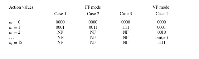
As shown in table 1, four cases are selected to perform DRL control with different feasible ranges of the actuator formations. Cases 1–3 belong to the FF mode. In this mode, the number of actuator columns involved in DRL control are selected a priori. During DRL control, those selected actuator columns are driven by the same trigger signal, fired synchronously. In cases 1, 2 and 3, the actuator columns involved in control gradually increase from
 $C_1$
, to
 $C_1 + C_2$
, and finally to
 $C_1 + C_2 + C_3 + C_4$
. As a comparison, case 4 belongs to the VF mode. In this mode, all four actuator columns are engaged in the DRL control. However, each actuator column is controlled independently by its own trigger signal, resulting in an asynchronous operation of the four actuator columns. Considering that each actuator column can freely choose between being active or silent, in total, 16 possible actions are available for the two-dimensional actuator array in case 4. The actuator formation code is related to the possible action value by a simple binary conversion:
 $FC=\text{bin}(a_t)$
.
Correspondence between actions and actuator formation codes in different cases; NF means ‘not feasible’.

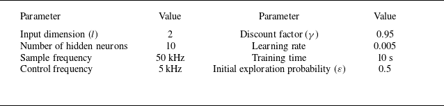
Table 2 summarises the setting of hyperparameters in DQN control. Following Zong et al. (Reference Zong, Wu, Li, Su and Liang2025), a discount factor
 $\gamma = 0.95$
is adopted to balance immediate and future rewards. The input dimension is fixed to 2, and the sampling frequency is set as 50 kHz, leading to a time interval 20
 $\unicode{x03BC} \textrm{s}$
between adjacent state elements. This interval is much shorter than the natural cavity resonance period (
 ${\sim}120$
 $\unicode{x03BC}$
s), enabling us to catch the short-period variation trend of the cavity flow. In each DRL control case, a complete wind tunnel run of 10 s is used to learn the optimal control strategy. For balanced exploration and exploitation, the entire operation time is divided into three stages, and the exploration rate
 $\varepsilon$
is assumed to be a piecewise-linear function of time. The first stage is the baseline stage (
 $t\leqslant 0.5$
s), with all actuators kept silent (
 $\varepsilon = 0$
,
 $a_t = 0$
), for measuring the baseline voltage statistics. The second stage corresponds to the training stage (
 $0.5\lt t\lt 9$
s), where the exploration rate decays linearly from 0.5 to 0 to encourage exploitation. In the last stage (evaluation stage,
 $9 \leqslant t\leqslant 10$
s), the trained neural network control law is executed deterministically (
 $\varepsilon =0$
) for performance assessment. This multi-phase acquisition approach enables simultaneous acquisition of the baseline and controlled flow statistics within one run. A prior test showed that this post-training immediate evaluation delivers performance identical to that obtained from a stand-alone evaluation run, and thus can reliably reflect the true capability of the learned policy. Physically, since the supersonic flow is a strongly convective flow, the disturbances can only propagate from upstream to downstream. When the upstream plasma actuation is withdrawn, fresh incoming supersonic flow will quickly wash out its hints as if nothing has happened. Consequently, the state of the supersonic cavity flow depends only on the control actions at this moment (and shortly before), unaffected by the actions far back in history (i.e. training stage).
Setting of the hyperparameters in DQN.

Except for the hot-wire measurement, high-speed schlieren imaging is carried out to capture the temporal evolution of the cavity shear layer under plasma actuation. The schlieren imaging system has a Z-type optical path, consisting of a high-speed charge-coupled device camera (Phantom V2512), two spherical mirrors (diameter 200 mm, focal length 2 m), a halogen lamp and a knife filter. The inter-frame time is set as 20
 $\unicode{x03BC}$
s (image acquisition frequency 50 kHz), consistent with the sample period of the raw hot-wire voltage. A 200 mm lens is mounted in front of the camera to image a field of view 176 mm
 $\times$
70.4 mm, with cropped sensor size 640
 $\times$
256 pixels
 $^2$
. The spatial resolution reaches 3.6 pixels per mm.
3. Results and discussion
This section is organised as follows. First, the temporal response of the cavity flow to pulsed-arc plasma actuation is analysed with the aid of schlieren imaging (§ 3.1). Then in § 3.2, the influence of different DRL settings is investigated in cases 1–4 for a representative cavity back-wall inclination angle of
 $30^\circ$
. Finally, § 3.3 compares the efficacy of DRL control at different inclination angles.
3.1. Response of cavity flow to pulsed-arc plasma
Figure 5 presents a representative temporal evolution of the cavity flow after one shot of the four PAPA columns, at
 $\theta = 30^\circ$
. To elucidate the complex interaction process, background subtraction is applied to the raw schlieren images (left-hand column), resulting in a feature-enhanced image of the large-scale structures (right-hand column). The time delay between plasma ignition and schlieren image acquisition is denoted
 $\Delta$
 $t$
. Using the cavity length and the freestream velocity as the reference scales for normalisation, a non-dimensional time can be derived:
 $t^\ast = \Delta t\times U_\infty /L$
. This metric represents the ratio of the distance travelled by plasma-induced disturbances in
 $\Delta$
 $t$
to the cavity length. Without plasma actuation (see figure 5
a i), the supersonic flow expands at the cavity leading edge, generating an expansion wave as marked by the yellow dashed line, and a reattachment shock forms due to flow compression at the cavity trailing edge.
Temporal response of the cavity flow to a single shot of pulsed-arc plasma actuation. The red arrows in (b i) indicate the streamwise positions of the four PAPA columns.

Shortly after the activation of the plasma actuator (
 $t^\ast = 0.2$
), electrical energy is rapidly deposited into the air gap in the form of arc heating, generating a series of bow-shaped shock waves and low-density thermal bubbles. During the subsequent time steps, the shock fronts propagate downstream and modulate the shear layer region by exciting the K–H instability. Specifically, at
 $t^\ast = 0.4$
, due to the shear of the boundary layer and entrainment of the mainstream, the thermal bubbles are elongated along the streamwise direction and start to interact with the shear layer. This progressive interaction induces a measurable lift-up of the shear layer. Morphologically, the most prominent control effect of plasma actuation is estimated to occur at
 $t^\ast = 0.6$
, where an obvious bump can be seen in the middle part of the shear layer (i.e.
 $x/D=2$
). Compared with the undisturbed baseline flow (see figure 5
a i), the lift-up of the thermal bulb into the main flow and the penetration of shear layer lower boundary into the recirculation zone will inevitably increase the momentum exchange between the cavity and the outside (Samimy & Elliott Reference Samimy and Elliott1990; Pantano & Sarkar Reference Pantano and Sarkar2002). At
 $t^\ast = 1$
, no hints of the plasma-induced shock waves can be found, and the shear layer thickness is elevated noticeably. Moreover, the shear layer tail is warped above the tip of the hot wire, in contrast with the baseline case in figure 5(a ii), where the middle of the shear layer is aligned with the hot wire. As expected from such a flapping motion, the instantaneous velocity measured by the hot wire will decrease between
 $t^\ast = 0.4$
and
 $t^\ast = 0.8$
.
Compared with our previous study in Zong et al. (Reference Zong, Wu, Li, Su and Liang2025), although similarities can be found in the control framework and plasma-induced disturbances (shock waves and thermal bulbs), noticeable differences exist in the actuation and mixing mechanisms. First, Zong et al. (Reference Zong, Wu, Li, Su and Liang2025) used plasma synthetic jet actuators. By pressurising the cavity with pulsed-arc discharge, high-speed fluids are ejected out of the orifice, which seed momentum disturbances to the shear layer. As a comparison, the present study utilises PAPA as the actuator. Localised thermal bulbs are produced via direct energy deposition, which virtually block the boundary layer and interact with the shear layer during downstream propagation. This thermal-based actuation mechanism contrasts with the aforementioned momentum-based actuation mechanism. Second, the research object in our previous work is a backward-facing step flow, where the shear layer develops almost freely without intense pressure feedback. In contrast, the present study investigates cavity flow, where the shear layer strongly interacts with the back wall, forming a complex feedback loop. Consequently, the plasma actuation in this study not only needs to excite the instabilities of the shear layer but also must couple with the inherent resonant frequency of the cavity, leveraging the natural feedback loop to enhance the mixing.
3.2. The DRL control under different actuation modes
Figure 6(a) compares the evolution of the filtered reward (denoted
 $\overline{r_t}$
, cut-off frequency 50 Hz) for the
 $\theta =30^\circ$
cavity across different DRL control cases. Regardless of the final achievement, the reward curves in different cases show similar variation trends: first a minor increase during the early exploration stage (
 $ 0.5 \lt t \lt 2$
s), then a rapid growth after sufficient experiences have been gained (
 $ 2 \lt t \lt 4$
s), and finally some fluctuations around a plateau value (
 $t\geqslant 4$
s). Note that in the initial exploration stage, the actions are almost random, and negligible rewards are earned, implying that plasma actuator should be fired at the right moment in order to manipulate the cavity flow towards the desired high-mixing state. For comparison, figure 6(b) shows the time evolution of the instant reward under OL periodic control, where the four actuator columns are operated synchronously at discharge frequency of
 $F_d = 5$
kHz. As a result, the instant reward fluctuates significantly between 0.16 and 0.25, and the time-averaged value is computed to be 0.22 (see the dashed black line in figure 6
a). This mean reward level achieved by OL control is only half of that achieved by the DRL control in cases 3 and 4, justifying the effectiveness of the proposed DRL control framework. To understand the behaviour of the plasma actuator, a metric called the actuator activation probability (
 $P_a$
) is defined. Mathematically,
 $P_a$
is computed as the ratio of the switch-on time in a given period to the total time of that period (set as 0.1 s in this study).
(a) Time evolution of the filtered reward under DRL control. (b) Instant reward variation obtained under OL periodical control. (c i–c iv) Activation probabilities of actuators
 $C_1{-}C_4$
in case 4. (d) Actuator activation probabilities in cases 1–3. (e) Power spectral density curves of the raw voltage signals.

In figure 6(d), the temporal variations of the actuator activation probability in synchronous actuation mode are plotted for cases 1–3. As a result, good agreement with the trend of the instant reward is found. The activation probabilities remain low (
 $\sim 0.2$
) initially, rise sharply at
 $t\approx 2$
s, and stabilise after
 $t=4$
s. Notably, with an increasing number of actuator columns, the steady-state reward increases monotonically. Figure 6(c i–c iv) present the column-specific activation probabilities for case 4. As shown in figure 6(c i–c iii), the first three columns (
 $C_1$
to
 $C_3$
) exhibit trends similar to those in cases 1–3. In contrast, the activation probability of
 $C_4$
shown in figure 6(c iv) rapidly shoots up to 0.8, after the training stage commences. Nevertheless, this behaviour fails to bring significant reward improvement, suggesting a limited control efficiency of the most upstream actuator column, presumably due to the long convection distance between the actuator and the cavity. For
 $2\lt t\lt 4$
s, the activation probabilities of
 $C_1{-}C_4$
maintain approximately the same growth rate, coinciding with the increase of instant reward in figure 6(a). At
 $t\approx 4$
s, DRL control enters the fine-tuning stage. Even though the reward cannot be improved any further, different actuation strategies are still being explored by the agent, as is evident from the staggered activation probability curves.
Figure 6(e) shows the power spectral densities of the raw voltage signals for both baseline and actuated cases. A dominant peak near
 $f=8.4$
kHz can be found, consistent with the resonance frequency values reported in our previous study (8.8 kHz) (Kong et al. Reference Kong, Wang, Zong, Wu, Liang, Tang and Qu2025a
) and in Oka et al. (Reference Oka, Ozawa, Handa and Nonomura2024) (8.6 kHz) for geometrically similar cavities. Compared with the baseline, DRL control elevates the power spectra overall, and the velocity fluctuation magnitudes in cases 1, 3 and 4 are increased by 21.2 %, 162.8 % and 312.6 %, respectively. Under OL control, a similar increase of the original spectral peak is observed, but slightly lower in amplitude when compared with cases 3 and 4. Additionally, for almost all the controlled cases, sharp peaks can be identified at 5 kHz and 10 kHz. Since after plasma actuation the natural resonance frequency of the cavity flow still lies in the range 8–9 kHz, these peaks are unlikely to be caused by the shift of flow resonance. Rather, they seem to be a direct spectral imprint from the control frequency.
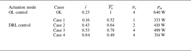
To comprehensively compare the performance of different control strategies, the time-averaged reward (
 $\bar {r}$
) and activation probability (
 $\overline{P_a}$
) during the evaluation stage (
 $9\leqslant t\leqslant 10\,\textrm{s}$
) are computed, as listed in table 3. Since the pulse energy remains unchanged during control, the time-averaged power consumed by the actuator array, namely the input power (denoted
 $P_{\textit{in}}$
), can be written as the product of the capacitor energy (
 $E_c$
), the number of actuator columns (denoted
 $N_c$
), and the number of pulses shot in one second. For cases of OL and DRL control, we have the following formulas for
 $P_{\textit{in}}$
:
Comparison of the mean reward and activation probability for different control strategies. Note that the metrics in DRL control are derived from the evaluation stage.

 \begin{equation} \left \{ \begin{array}{l} P_{\textit{in}} = E_c\,N_c\,F_d, \\ \displaystyle P_{\textit{in}} = E_c\,N_c\,F_c\,\overline{P_a}. \end{array} \right . \end{equation}
Here, the product of control frequency and mean activation probability in DRL control (i.e.
 $F_c\,\overline{P_a}$
) bears a meaning similar to the discharge frequency in OL control. Consequently, as shown in table 3, the OL control case consumes the highest input power, yet its mean reward is much lower than the best scenario in DRL control (case 4).
(a) Time evolution of the actuator formation selection probabilities during the course of learning in case 4. (b) Reward distributions pertaining to different actions (i.e. actuator formations). The top and bottom edges of the white rectangles correspond to the locations of the 75th and 25th percentiles, respectively.

In cases 1–3, both
 $\bar {r}$
and
 $\overline{P_a}$
increase monotonically with the number of activated actuator columns. This indicates that in the synchronous actuation mode, the enhancement in reward essentially comes at the cost of utilising more actuators and increased power consumption. As a comparison, in the VF mode where the controller is allowed to choose freely from 16 actions (case 4), DRL finds the highest
 $\bar {r}$
by utilising the lowest input power. This clearly demonstrates the superiority of adaptive-formation actuation over FF actuation. Intuitively, greater freedom given to DRL control increases its potential to discover improved control laws.
Figure 7(a) presents a probability heat map illustrating the time evolution of different actuator formations during VF control (case 4). The left-hand vertical axis enumerates the 16 actions, while the right-hand panel sketches the corresponding actuator formation code together with the activated actuator columns. In the baseline stage
 $t\lt 0.5$
s, all actuators remain inactive (
 $FC = 0000$
), as expected. During the initial exploration phase
 $0.5\lt t\lt 2\,\textrm{s}$
, the actuator formation sticks on 1000 and only
 $C_4$
is active, with minimal usage of other actuator columns. Between
 $t = 2$
s and
 $t=9$
s, the actions alternate dynamically (range 1–15), with no dominant actuator formation emerging. This evolution pattern fully complies with the column-specific activation probabilities shown in figure 6(d). During the course of learning, action values 2, 4 and 8 (
 $FC = 0010$
, 0100 and 1000) are rarely utilised. As a comparison, action values 1, 3 and 6 (
 $FC = 0001$
, 0011 and 0110) are selected frequently, indicating that these actuator formations are crucial in DRL control.
In figure 7(b), the reward distributions pertaining to different actions (i.e. actuator formations) are visualised as violin plots. To obtain these distributions, the reward data are first split into 16 subsets according to their respective actions, and kernel density estimation is then applied to each subset. In the baseline case
 $a_t = 0$
, the instant reward exhibits an approximate symmetric distribution with respect to zero (black dashed line), as prescribed by (2.6). By contrast, all other actuator formations exhibit an upward shift of the reward distribution with respect to the baseline, and the majority of the reward values are concentrated between 0 and 2, leaving only a few samples exhibiting negative reward. In terms of the mean reward magnitude, an approximate increasing trend of
 $r_t$
with the number of actuator columns can be picked. Even though, no deterministic conclusion in terms of the optimal actuator formation should be drawn, since DRL control is a closed-loop adaptive control, and the optimal actuator formation depends on the instantaneous flow state.
3.3. Comparison of different inclination angles
Since the previous subsection has proved that the DRL control strategies in cases 1 and 2 are suboptimal, this subsection examines the performance of only cases 3 and 4. As shown in figure 8(a), the evolution trends of the filtered rewards for cavities with different inclination angles exhibit characteristics similar to those shown in figure 6(a). Specifically, three phases – including an initial exploration phase, a rapid growth phase and a plateau phase – can be clearly identified, and higher rewards are achieved by cavities with lower inclination angles. According to the mean reward plotted in figure 8(b), the control efficacy decreases with increasing
 $\theta$
, and VF DRL control strategy in case 4 consistently outperforms the synchronous DRL control strategy in case 3. At large inclination angles, the relatively weak control efficacy can be attributed to the intrinsically strong flow instability in baseline condition (Vikramaditya & Kurian Reference Vikramaditya and Kurian2009). Specifically, due to the intense acoustic feedback provided by the back wall, even without plasma actuation, the shear layer can also be excited by natural disturbances, which eventually leaves a small margin for the plasma actuator to improve. The power spectral density profiles in figures 8(c) and 8(d) provide direct evidence for the above explanation. Although the dominant frequency (
 $f=8.4$
kHz) remains invariant due to identical cavity length and depth, the spectrum peak does increase noticeably at higher inclination angles.
(a) Time evolutions of the filtered rewards for cavities with different back-wall inclination angles. (b) Comparison of the mean rewards in the evaluation stage. (c) Power spectrums of the voltage signals obtained at
 $\theta =45^\circ$
. (d) Power spectrums of the voltage signals obtained at
 $\theta =90^\circ$
.

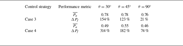
Table 4 summarises the mean activation probability and relative increase of spectrum peak in different cases (denoted
 $\Delta P_{\!f}$
). As a result,
 $\Delta P_{\!f}$
decreases monotonically with increasing
 $\theta$
, consistent with the variation of mean reward, yet the mean activation probability remains almost invariant with the inclination angle. Compared with the synchronous control strategy in case 3, VF DRL control is capable of elevating the spectrum peak to a much higher level, three times higher than the former at
 $\theta =90^\circ$
. Moreover, this higher control authority does not incur higher power consumption. The mean activation probability in case 4 is approximately 0.5, much lower than that of the synchronous control (case 3,
 $\overline{P_a}=0.76{-}0.78$
). This once again illustrates that with a smart on-demand control strategy, not only can the control effectiveness be improved, but also the actuator power consumption can be reduced.
List of the mean activation probability and the relative improvement of spectrum peak under different control strategies.

Since in schlieren imaging, the image greyscales are correlated with the integral of the density gradients along the light path, the density fluctuation intensity in the cavity flow field can be quantified by the standard deviation of the schlieren image greyscales (denoted
 $I_{\textit{std}}$
). As shown in figure 9(a), in the baseline condition
 $\theta =30^\circ$
, strong density fluctuations are concentrated within the shear layer and reattachment shock, while relatively weak fluctuations reside in the upstream boundary layer and expansion waves. Based on the wall-normal profile of the greyscale fluctuation amplitude extracted at
 $x/D = -2$
, the boundary layer thickness is estimated to be 3.0 mm (see Appendix A for details). Plasma-induced density fluctuation variations (denoted
 $\Delta I_{\textit{std}}$
) can be visualised by subtracting the baseline distribution of
 $I_{\textit{std}}$
from the
 $I_{\textit{std}}$
obtained in actuated conditions. After plasma actuation (see figure 9
d), four inclined wavefronts are emitted from the vicinity of plasma actuator columns, corresponding to the density perturbations generated by the outward propagation of arc-induced shock waves. Except for these regions, the streamwise convection of thermal bulbs significantly enhances the fluctuations in the upstream boundary layer and the downstream shear layer. With increasing inclination angle (figures 9
a–c), the baseline shear layer density fluctuation amplitude increases, due to the enhanced acoustic resonance in the cavity. As a comparison, the plasma-added greyscale fluctuation, which can be judged from the variation of shear layer thickness, exhibits a decreasing trend with the inclination angle. These phenomena are consistent with the results in figure 8 and table 4.
(a–c) Greyscale fluctuation of the schlieren images in the baseline condition. (d–f) Variations of the greyscale fluctuation amplitudes caused by plasma actuation in case 4. From top to bottom, the inclination angle corresponding to each row is
 $\theta =30^\circ ,45^\circ, 90^\circ$
.

Figure 10 compares the temporal responses of the large-scale flow structures to a single shot of four-column plasma actuation at
 $\theta =30^\circ$
and
 $90^\circ$
. Analogous evolution mechanisms are shown at different inclination angles. Specifically, upon plasma actuation, thermal bulbs are produced in the electrode zone, which push the local streamlines upwards by the thermal blockage effect, causing a thickened boundary layer. Then these bulbs are elongated due to the shear stress during downstream propagation, modulating the shear layer by exciting the K–H instability. Compared with the low inclination angle
 $\theta =30^\circ$
, the case
 $\theta =90^\circ$
exhibits a significantly higher shear layer lift-up. In Wang & Cao (Reference Wang and Cao2025), upstream wavy walls were used to enhance the fuel–jet mixing efficiency by producing streamwise vortices. Although effective, such passive flow control devices can incur total pressure loss. The arc plasma actuator matrix proposed in this study, in contrast, is an on-demand plasma actuation offering two merits. First, no total pressure loss is induced when being idle. Second, the streamwise/spanwise actuation wavelength can be adjusted dynamically according to the changes of external flow conditions.
Time evolution of the plasma-induced large-scale structures at different back-wall inclination angles: (a)
 $\theta =30^\circ$
, (b)
 $\theta =90^\circ$
.

Visualisation of the final control law obtained by DRL in case 3.

4. Closed-loop control mechanism
In this section, the closed-loop control mechanisms in cases 3 and 4 are discussed by answering three questions. First, from the perspective of control law interpretability, when would the controller act? Second, from the perspective of system dynamics, how does the state of flow evolve under plasma actuation? Finally, from the perspective of reinforcement learning, why would the learnt control law benefit?
4.1. Synchronous FF actuation in case 3
Since the state vector
 $\boldsymbol{x}$
only incorporates two elements (denoted
 $x_1$
and
 $x_2$
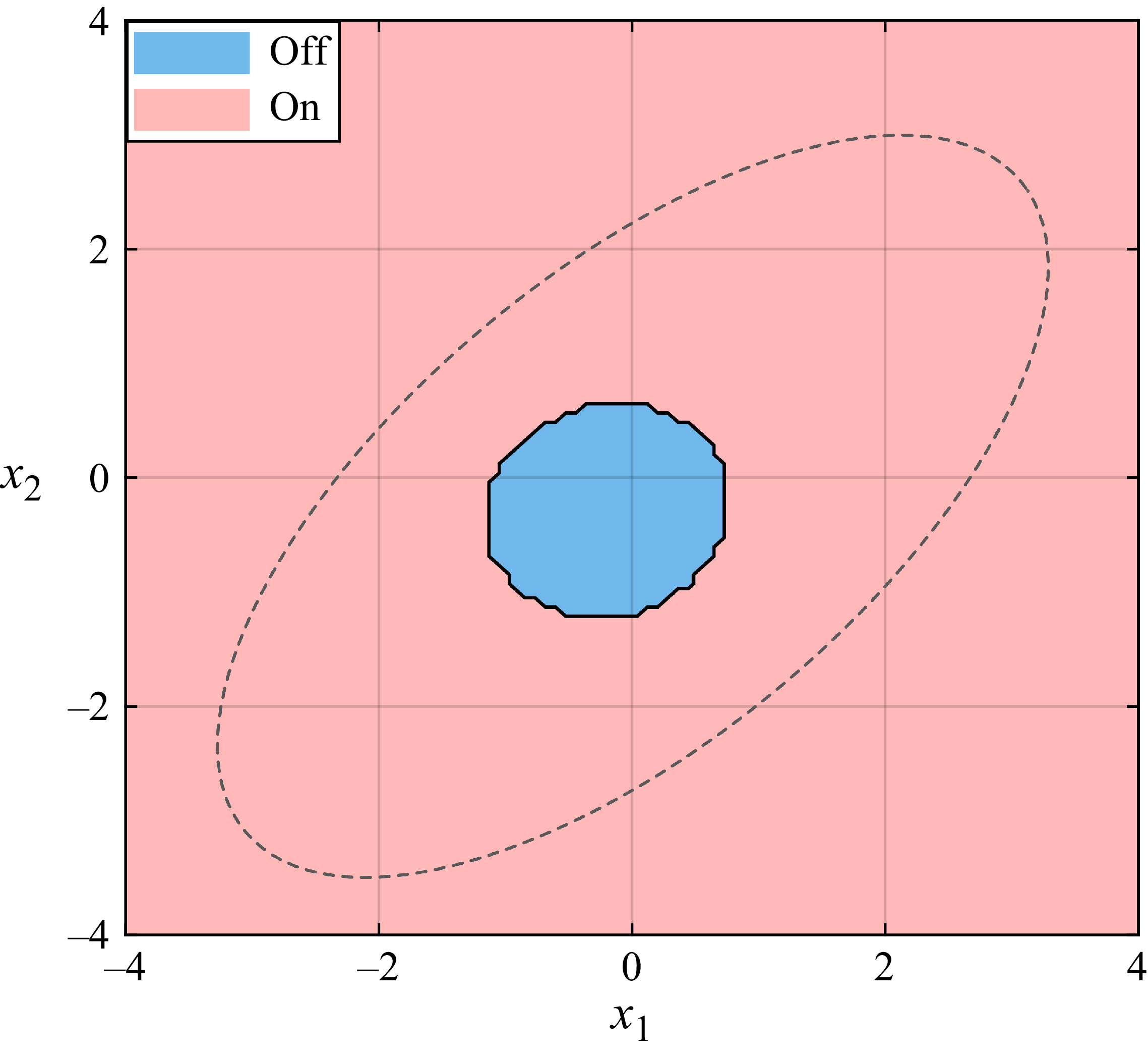
), the control law parametrised by the RBF network can be readily visualised by a two-dimensional map, with the action values shown as a contour. Figure 11 shows the final control law obtained by DRL pertaining to case 3, where the dashed black ellipse delineates the feasible zone of the state vector. This ellipse is drawn from the outer envelope of the state vectors in the
 $x_1{-}x_2$
space, taking the data obtained in both baseline and controlled conditions into account (see figure 12
a). Since only two actions are involved, the logic in this scenario is relatively simple. Specifically, plasma actuator should be activated when the state vector lies outside the blue circle centred at (
 $-0.2, -0.2$
), and vice versa. The diameter of the circle (
 $\approx 1.5$
) is much less than the feasible range of the state vector, thus the actuation probability is higher than 0.5. Physically, since the two elements of the state vector are essentially the dimensionless hot-wire voltage reflecting how much the instantaneous location of the shear layer deviates from its mean, the final control law obtained in case 3 can be interpreted as a threshold actuation.
(a) Cluster of the state vectors in a two-dimensional space. (b,c) State transition probability matrices in baseline and case 3. (d) Plasma-induced state transition probability variation. (e) Cluster occurrence probability and activation probability. ( f) Comparison of the cluster-specific reward distributions in baseline and case 3.

In Kaiser et al. (Reference Kaiser, Noack, Cordier, Spohn, Segond, Abel, Daviller, Östh, Krajnović and Niven2014) and Maceda et al. (Reference Maceda, Varon, Lusseyran and Noack2023), the dynamics of flow were analysed by a cluster-based Markovian model. Inspired by their studies and to understand how the flow states transfer in our scenario, the two-dimensional state vectors recorded during the course of learning (
 $\boldsymbol{x}$
) are classified into four clusters (denoted
 $\varOmega _{i}$
,
 $i= 1, 2, 3, 4$
) by a classical algorithm called K-means clustering (Lloyd Reference Lloyd1982). The choice of this small cluster number is justified by the low input dimension of the state vector (2). Further increasing the cluster number indeed can reduce the residual in clustering analysis, however will significantly complexify our subsequently state transfer dynamics. The transition probability from the
 $i\rm th$
cluster
 $\varOmega _i$
to the
 $j\rm th$
cluster
 $\varOmega _{\!j}$
is defined by
 \begin{equation} P_{i,j}=P(\boldsymbol{x}_t\in \varOmega _{\!j}\,|\,\boldsymbol{x}_{t-1}\in \varOmega _i). \end{equation}
Figure 12(a) shows the cluster results of state vectors, where each dot represents a sample point. As is evident, the joint distribution of
 $x_1$
and
 $x_2$
exhibits an elliptical pattern, with most data points concentrated in the first and third quadrants. Clusters 2 and 4 occupy the two ends of the ellipse, while clusters 1 and 3 share the central region. Connecting with the shear layer dynamics described in the last section, we can infer that cluster 2 corresponds to the scenario where the shear layer penetrates deep into the recirculation zone (figure 5
aii), leaving the hot wire exposed in the freestream. By analogy, cluster 4 implies that the shear layer has been elevated high above the hot wire. Clusters 1 and 3 represent transient flapping motions of the shear layer since the sign of the dimensionless voltage has been changed.
The cluster transition probability matrices in baseline and case 3 are plotted in figures 12(b,c). Under the baseline situation, clusters 1–3 form a closed transition loop (
 $\varOmega _1\rightarrow \varOmega _2\rightarrow \varOmega _3\rightarrow \varOmega _1$
), while cluster 4 transfers to clusters 1 and 2 in approximately equal probability. After plasma actuation, cluster 4 is also incorporated in the aforementioned transition loop, and a clear path
 $\varOmega _1\rightarrow \varOmega _2\rightarrow \varOmega _3\rightarrow \varOmega _4\rightarrow \varOmega _1+\varOmega _2$
can be identified. Notably, the alternative branching paths
 $\varOmega _2\rightarrow \varOmega _3+\varOmega _4$
and
 $\varOmega _4\rightarrow \varOmega _1+\varOmega _2$
now possess comparable probabilities. Furthermore, a direct transition
 $\varOmega _4\rightarrow \varOmega _2$
emerges. This represents a non-continuous state jump where the shear layer transitions from a highly elevated position (
 $\varOmega _4$
) directly to a cavity penetration (
 $\varOmega _2$
), which can be attributed to the flapping motion induced by the plasma actuation. To highlight the impact of plasma actuation, the differential probability matrix (
 $\Delta P_{i,j}$
) computed from the difference of probability values in baseline and actuated conditions is further shown in figure 12(d). Obviously, plasma actuation tries to eliminate the transition towards clusters 1 and 2, while striving to increase the transitions towards clusters 3 and 4.
A direct consequence of the above state transition dynamics is the change of cluster occurrence probability (denoted
 $P_\varOmega$
). Figure 12(e) plots the distributions of
 $P_\varOmega$
in baseline and actuated conditions (
 $P_{\varOmega ,BL}$
versus
 $P_{\varOmega ,AT}$
), as well as the cluster-wise activation probabilities (
 $P_\varOmega$
). As expected from the analyses of differential state transition map, the occurrence probabilities of clusters 1 and 2 are reduced noticeably by plasma actuation, and these saved occurrence chances eventually flow to clusters 3 and 4. Figure 12( f) presents the reward distributions in different clusters (shaded area) and the cluster-specific mean reward. The baseline and actuation cases are represented by light blue and red colours, respectively. Regardless of plasma actuation, cluster 4 always exhibits a reward distribution higher than clusters 1–3, reflecting inherently stronger velocity fluctuations associated with that flow state. Plasma actuation globally shifts the reward distributions upwards, increasing the mean reward, yet the distribution shape seems to be invariant. The most significant improvement of the reward occurs in cluster 2.
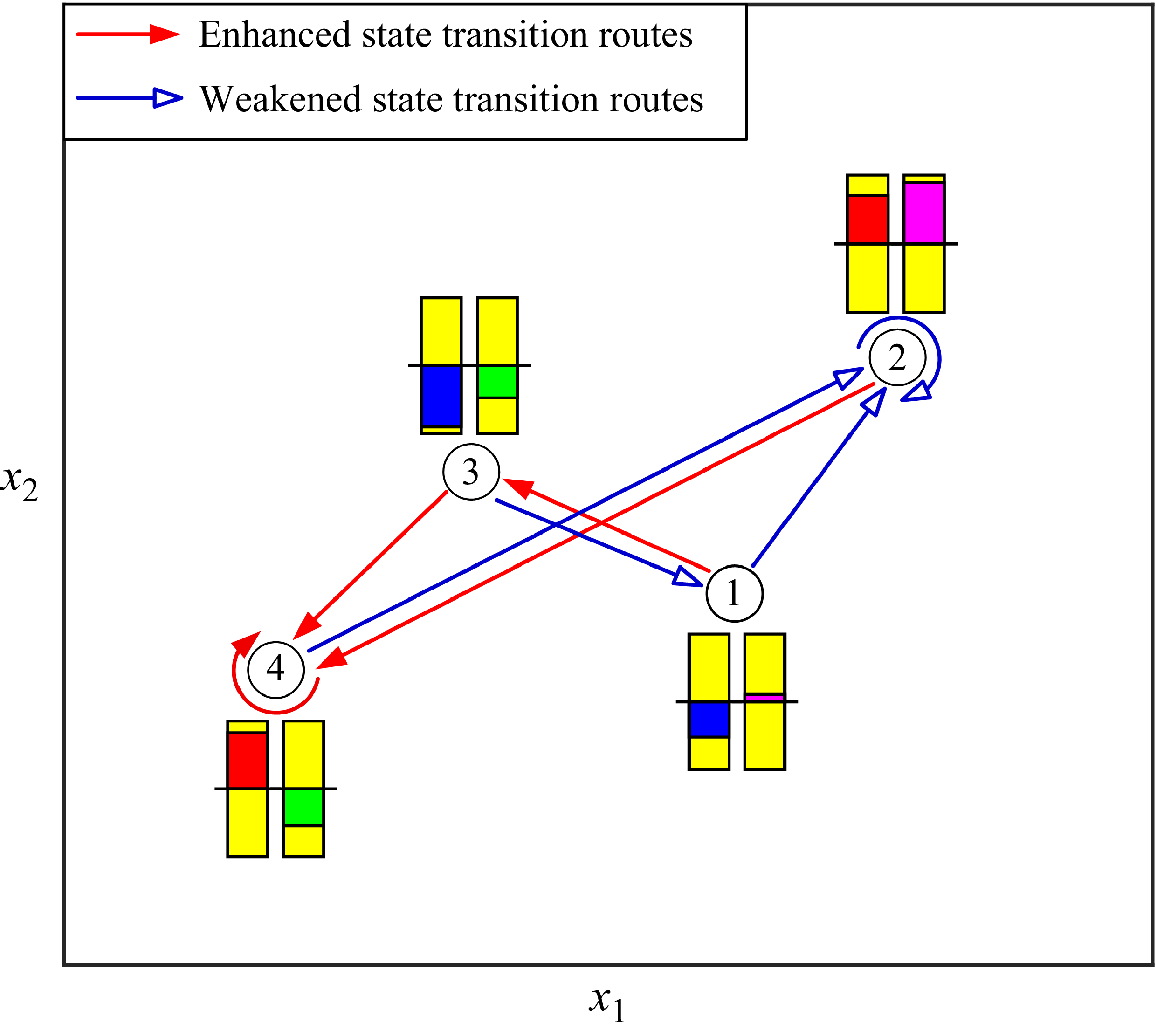
Sketch of the state transition graph in case 3. The left-hand bar indicates the relative magnitude of the reward with respect to the global mean reward (low to high by blue to red). By analogy, the right-hand bar represents the relative activation probability with respect to the global mean activation probability (low to high by green to pink).

Based on the differential transition probability matrix shown in figure 12(d), a directional state transition graph can be sketched, which visually reveals how DRL control redistributes the states among clusters. As shown in figure 13, enhanced transition routes with
 $\Delta P_{i,j}\gt0.1$
and weakened transition routes with
 $\Delta P_{i,j}\lt-0.1$
are sketched as red arrows and blue arrows, respectively. Insignificant variations with
 $|\Delta P_{i,j}|\lt0.1$
are not taken into account. For better linkage with the flow physics, the corresponding flow scenario is sketched based on the state vector value at each cluster centre. As a result, the centre of cluster 2 features large positive values of
 $s_1$
and
 $s_2$
, indicating that the shear layer should be below the hot-wire tip, leaving the latter exposed to the main freestream. By analogy, cluster 4 denotes the scenario where the shear layer is high above the hot-wire tip, and clusters 1 and 3 represent the intermediate scenarios where the shear layer has just crossed the tip (cluster 1, downward crossing; cluster 3, upward crossing). The DRL control enhances the inflow transitions towards the high-reward low-actuation cluster (cluster 4), meanwhile reducing its outgoing transitions towards cluster 1. These variations effectively promote the upward motion of the cavity shear layer, leading to mixing enhancement.
4.2. Asynchronous VF actuation in case 4
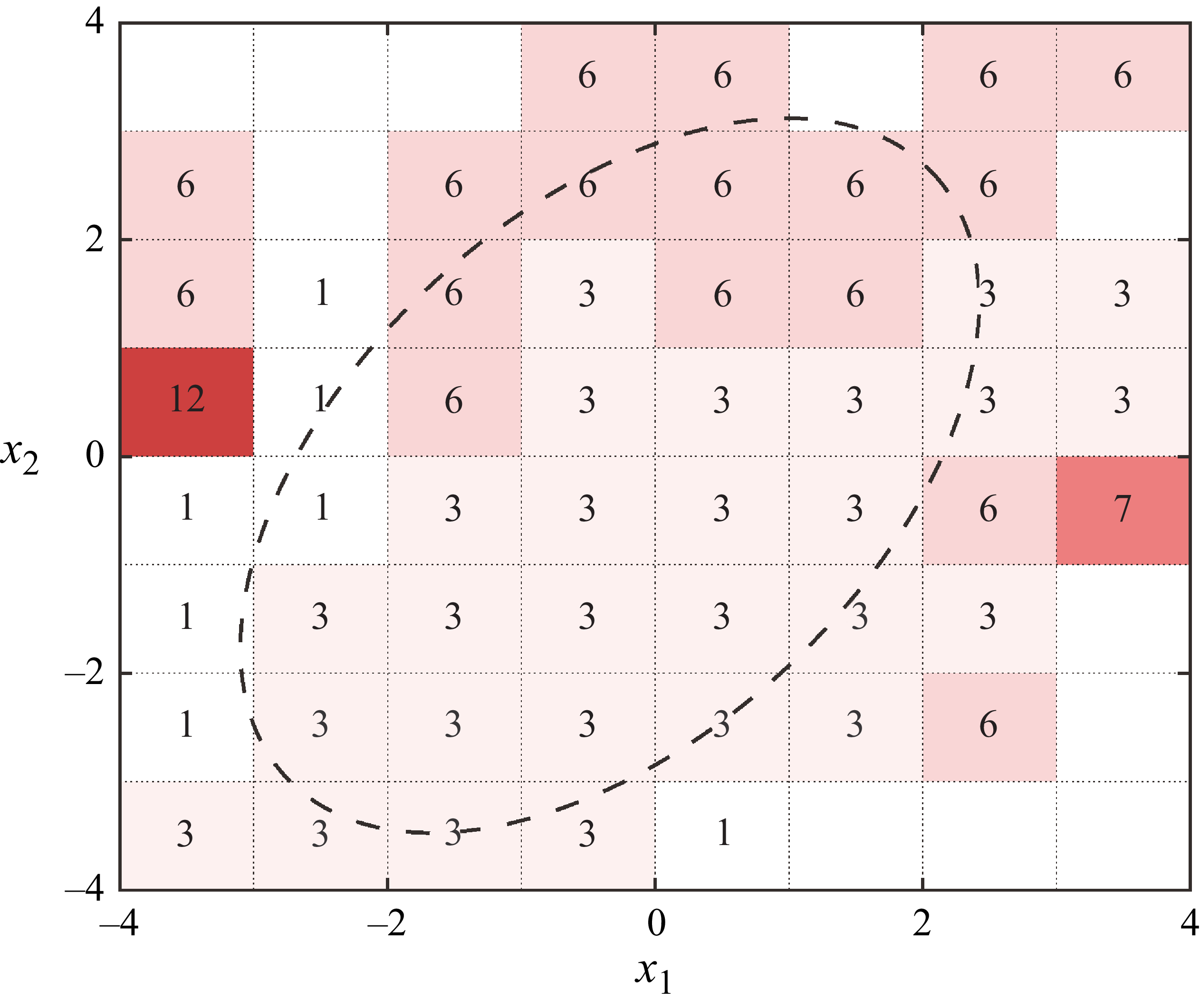
Figure 14 visualises the final control law obtained by asynchronous control in case 4. To ease interpretation, the entire two-dimensional space spanned by
 $x_1$
and
 $x_2$
is split into a grid, with step size 1, and the dominant action value within each grid is directly labelled. The dashed black line defines approximately the feasible state zone (see figure 12
a), beyond which negligible state vectors can be found. As a result, within the feasible zone, action values 1, 3 and 6 are selected frequently, corresponding to formation codes
 $FC = 0001$
, 0011 and 0110. In terms of the area, action value 3 occupies approximately 51 % of the feasible zone. These results are consistent with the temporal evolution of formation code shown in figure 7(a).
Visualisation of the final control law obtained by DRL in case 4.

(a) State transition probability in case 4. (b) Plasma-induced state transition probability variation. (c) Cluster occurrence probability and activation probability. (d) Comparison of the cluster-specific reward distributions in baseline and case 4.

The state transition probability matrix and the plasma-induced probability variation pertaining to case 4 are plotted in figures 15(a,b). Similar to the synchronous control in case 3, a cyclic transition path
 $\varOmega _1\rightarrow \varOmega _2\rightarrow \varOmega _3\rightarrow \varOmega _4\rightarrow \varOmega _2$
can be identified. Plasma actuation suppresses transitions to clusters 2 and 1 as well as promoting transitions to cluster 4. This, consequently, leads to a noticeably reduced occurrence probability in cluster 2, and a slightly increased occurrence probability in cluster 4, as is evident in figure 15(c). As with the activation probability, an approximately even distribution across different clusters is observed in case 4, different from the synchronous control in case 3. Figure 15(d) compares the cluster-specific reward distributions before and after plasma actuation. Qualitatively, the shapes and variation trends of these distributions closely follow those in figure 12. However, quantitatively, in case 4 the reward improvement at
 $\varOmega _2$
is 50 % higher than that in case 3, which partially explains the superior control authority of the former.
Figure 16 summarises the plasma-induced variations of the state transition dynamics in case 4. Similar to the analysis in the previous subsection, cluster 4 delivers the highest reward, followed by cluster 2. Clusters 1 and 3 receive below-average rewards. Regarding the inter-cluster transition dynamics, except for the enhanced inflow transition routes
 $\varOmega _3\rightarrow \varOmega _4$
and
 $\varOmega _2\rightarrow \varOmega _4$
, the self-sustaining probability of cluster 4 is also enhanced, indicating that DRL control tries to trap the states in cluster 4. As a comparison, the transition routes towards cluster 2 together with its self-sustaining route are weakened noticeably, meaning that DRL control strives to evacuate the state in cluster 2. Such a distinct behaviour may be ascribed to the different activation probabilities. Specifically, although cluster 2 shares comparable reward levels with cluster 4, its mean activation probability is much higher. Therefore, quenching the states in cluster 2 is beneficial to the reduction of overall power consumption. Cluster 3 seems to be a springboard, relaying the states from the low-reward cluster (cluster 1) towards the high-reward cluster (cluster 4).
Sketch of the state transition graph in case 4. The plotting styles in figure 13 are inherited.

Until now, the critical question of ‘why would the learnt control law benefit’ raised at the start of § 4 remains unresolved. To answer this question, we need to combine the above analyses. Specifically, the increase of time-averaged reward in DRL control can be attributed to two aspects. One is the redistribution of states among different clusters, and the other is the redistribution of rewards within a particular cluster. Mathematically, the following equation for the global-mean reward can be formulated:
 \begin{align} \left \lbrace \begin{array}{l} \bar {r}=\displaystyle\sum\nolimits_{k=1}^{4}{P_\varOmega (k)\boldsymbol{\cdot}\bar {r}_k}, \\[9pt] \bar {r}_k=\displaystyle\int _{-\infty }^{+\infty }{f(r\,|\,\boldsymbol{x}\in \varOmega _k)\boldsymbol{\cdot} r\boldsymbol{\cdot}{\rm d}r} . \end{array} \right . \end{align}
Here,
 $r_k$
denotes the expectation of cluster-specific mean reward, and
 $f(r\,|\,\boldsymbol{x}\in \varOmega _k)$
represents the probability density function of the instant reward pertaining to cluster
 $\varOmega _k$
. Applying the above equation to the data shown in figures 12 and 15, the reward improvement secrets in DRL control become clear. First, the occurrence probability of the high-reward cluster (i.e. cluster 4) is increased. Second, the mean reward of each cluster is improved ubiquitously.
5. Conclusion
In this study, experimental DRL control of a supersonic cavity flow is conducted for the first time at Mach 2 at Reynolds number
 $\textit{Re}=2\times 10^6$
. Controllable thermal disturbances are produced by a specially designed PAPA matrix, and real-time flow sensing is achieved by a supersonic hot-wire sensor. The neural network control law that outputs the instantaneous actuator formation based on the flow state is optimised by the classical DQN algorithm. By analysing the performance of DRL in different operation modes and cavity geometries, meaningful conclusions are reached, as follows.
Under the baseline condition, the cavity resonance intensity grows monotonically with the back-wall inclination angle. Plasma actuation is able to thicken the incoming boundary layer by the thermal blockage effect, and induce a meandering motion of the shear layer via exciting the K–H instability. In a typical DRL control process, the instant reward first exhibits a minor increase, then climbs rapidly, and finally reaches a plateau. Less than 10 s is needed to obtain a converged control law, regardless of the operation mode. For the FF operation mode, the final reward increases with the number of activated actuator columns, but at the cost of growing actuator power consumption. As a comparison, in the asynchronous VF operation mode, a much higher reward is achieved with less actuator power usage. Increasing the back-wall inclination angle leads to a degradation of the control effectiveness of the plasma actuator, largely due to the intrinsically strong flow instability in the baseline condition. With respect to the baseline, DRL control elevates the power spectra of the hot-wire velocity as a whole, and the total fluctuation magnitude is almost tripled by VF actuation.
The final control law obtained in the synchronous FF operation mode can be interpreted as a threshold control strategy, dictating that the plasma actuator should be fired when the corresponding state vector lies outside a blue circle centred at [
 $-2, 2$
]. Plasma actuation is able to significantly alter the state transition dynamics of the cavity flow, and improvement of the mean reward is realised by eliminating the transition towards low-reward clusters while boosting the transition towards high-reward clusters. Additionally, the reward distributions at different clusters are elevated as a whole by FF actuation. Under asynchronous VF operation mode, formation code 0011 is selected approximately half of the time, and a cyclic transition path can be identified in the cluster transfer graph. Compared with FF actuation, although the cluster-specific reward distribution shows a similar shape in the VF mode, the expectation of the instant reward is elevated by 50 %, explaining the superior control authority of VF actuation.
In the future, the following works are recommended. First, high-fidelity numerical simulations or time-resolved particle imaging velocimetry diagnostics should be carried out to elucidate the dynamics of plasma-induced coherent vortical structures. Second, the performance of DQN should be compared with other machine learning control algorithms, such as linear genetic programming and DDPG.
Supplementary movies
Supplementary movies are available at https://doi.org/10.1017/jfm.2026.11212.
Funding
This work was sponsored by the National Natural Science Foundation of China (nos 52441602, U2341277, 12572319, 52488101).
Declaration of interests
The authors report no conflict of interest.
Appendix A. Properties of the incoming boundary layer
In the present study, the boundary layer upstream of the cavity is confirmed to be a fully developed turbulent boundary layer after evolving along the fore-plate. The total pressure, total temperature and freestream velocity of the boundary layer are measured to be 78.4 kPa, 293 K and 510 m s−1, respectively. The detailed boundary layer velocity profile is not diagnosed, due to the absence of appropriate measurement equipment. However, by analysing the high-speed schlieren images, we are able to estimate the boundary layer thickness prior to plasma actuation. Specifically, strong greyscale fluctuations caused by the unsteady nature of turbulence are obvious in the upstream boundary layer region, as shown in figure 17(a). To quantify the boundary layer thickness, the vertical profile of
 $I_{\textit{std}}$
is extracted at
 $x/D = -2$
, corresponding to 180 mm downstream of the plate leading edge. As is evident in figure 17(b),
 $I_{\textit{std}}$
decays monotonically with increasing wall-normal height. In particular, at
 $y \geqslant3$
mm, the greyscale fluctuation intensity already drops to a rather low level, close to that in the freestream. This indicates that the boundary layer thickness (denoted
 $\delta$
) at this location is approximately 3 mm.
(a) Greyscale fluctuation amplitude of the schlieren images in the baseline condition. (b) Greyscale fluctuation profile extracted at
 $x/D = -2$
.

Theoretically, using the reference temperature method, the nominal thickness of the turbulent boundary layer developing over a flat plate can be calculated by the equation (White & Majdalani Reference White and Majdalani2006)
 \begin{align} \left \{ \begin{array}{l} \displaystyle \frac {T^\ast }{T_\infty }=0.45+0.55 \boldsymbol{\cdot} \frac {T_{w\textit{all}}}{T_\infty }+0.16 \times 0.89 \times \left(\frac {\gamma _0-1}{2}\right)\textit{Ma}^2, \\[10pt] \displaystyle \frac {\delta }{x} = \frac {0.37}{\textit{Re}^{0.2}_x}\boldsymbol{\cdot}\left(\frac {T^\ast }{T_\infty }\right)^{0.8}\!, \end{array} \right . \end{align}
where
 $T_\infty$
and
 $T_{w\textit{all}}$
represent the freestream static temperature and wall static temperature, respectively. Under the adiabatic wall assumption, both values are identical at 160 K;
 $\gamma _0$
denotes the specific heat ratio,
 $T^\ast$
is the reference temperature, and
 $\textit{Re}_x$
is the Reynolds number based on the reference plate length and freestream parameters. Substituting these values into the above equation, the theoretical value of the boundary layer thickness is calculated to be 3.5 mm, which is close to the value extracted from high-speed schlieren imaging.