1. Introduction

Nash equilibriums (and Nash equilibrium refinements such as evolutionary stability) are often relied on to explain behavior in strategic interactions. Two agents are in Nash equilibrium if they are each using a strategy that is a best response to the other’s strategy. In such a situation, neither player can gain by switching her strategy; given what her opponent is doing, she’s doing the best she can do. A famous instance of a scientific explanation that relies on the notion of Nash equilibrium is Fisher’s (Reference Fisher1930) explanation of the fact that in many species the sex ratio at reproductive age is approximately 1:1 (see also Hamilton Reference Hamilton1968; Sober Reference Sober1983). Fisher noted that if a population is at an even sex ratio, then there is no reproductive advantage to producing offspring in proportions that violate the ratio. This means that a 1:1 sex ratio is a Nash equilibrium. He also noted that if a population deviates away from this ratio, then there will be a reproductive advantage for producing members of the scarcer sex. In modern terminology, this means roughly that a 1:1 sex ratio is not only a Nash equilibrium but also an evolutionarily stable strategy. These equilibrium-based observations are thought to have explained why approximately even sex ratios are prevalent in nature. This style of explanation is prevalent throughout all disciplines that use game theory. Explanations in microeconomics, for instance, often begin and end by demonstrating that a behavior is a Nash equilibrium.Footnote ¹

In order for Nash equilibriums to provide satisfying explanations of behavior, however, there must be some underlying story as to why actors choose to behave in such a way that their joint behaviors are in equilibrium. A popular approach to this issue takes inspiration from theories of learning and evolution. Instead of focusing on static equilibriums, the game is embedded into a dynamical system engineered to capture the essence of differential reproduction or social learning. A growing body of mathematical results helps to link the behavior of these dynamical systems to the predictions of static equilibrium concepts, such as Nash equilibriums. A well-known collection of theorems, for instance, proves that in some types of games, standard continuous-time evolutionary and learning dynamics are guaranteed to lead to Nash equilibriums (see, e.g., Cressman Reference Cressman2003, theorem 2.7.4).

But these theorems only cover somewhat special cases, and when a system does not fit the theorems’ constraints, convergence to Nash equilibrium is not guaranteed. For example, it is known that, in some games with four strategies, the continuous-time replicator dynamic exhibits chaotic behavior in which orbits converge to strange attractors (Arneodo, Coullet, and Tresser Reference Arneodo, Coullet and Tresser1980; Schnabl et al. Reference Schnabl, Stadler, Forst and Schuster1991; Skyrms Reference Skyrms1992). An even more complex form of behavior—Hamiltonian chaos—is seen in the replicator dynamic in both four-dimensional rock-scissors-paper games (Sato, Akiyama, and Farmer Reference Sato, Akiyama and Farmer2002) and 52-dimensional zero-sum signaling games (Wagner Reference Wagner2012). These systems do not lead to Nash equilibrium play and therefore illustrate that the dynamic approach to studying behavior in games does not unequivocally vindicate a single-minded focus on static equilibrium concepts.

But how deep do these nonconvergence results go? In this article, I demonstrate that they arise in the simplest possible case: ordinary two-strategy games with a single equilibrium. Despite having an exceedingly simple state space—the interval —and just a single equilibrium, agents may not converge to the equilibrium. A natural family of discrete-time imitation dynamics exhibits chaotic behavior in these simple games. This family, called the discrete-time imitative logit dynamic, was first introduced by Cabrales and Sobel (Reference Cabrales and Sobel1992), who noted that, in contrast to the discrete-time replicator dynamic, the limit points of the discrete-time i-logit dynamic are rationalizable strategies.Footnote ² This dynamic is parameterized by a “myopic rationality” term that influences the probability with which agents choose to imitate another player with a higher payoff. For low values of this parameter, the dynamic resembles the not-so-rational replicator dynamic. For high values of this parameter, the dynamic resembles the highly rational best-response dynamic. Thus, the discrete-time i-logit family allows one to systematically study the behavior of a range of boundedly rational players.

A derivation of this dynamic, along with a list of motivations for studying its behavior, is presented in section 2. Its behavior in a game with a single isolated interior evolutionarily stable strategy is illustrated in section 3. The dynamic follows the period-doubling route to chaos as the myopic rationality parameter is varied from low to high. Thus, the route from low rationality learning to high myopic rationality involves a journey through regimes of complicated limit cycles and chaotic attractors. Furthermore, the dynamic also undergoes the period-doubling route to chaos as the payoffs of the game are varied. These results show that convergence to equilibriums cannot be guaranteed in even the most simple games, and one therefore perhaps ought to view the predictions of static equilibrium theory with some skepticism. Without a robust model suggesting that actors do in fact learn Nash equilibrium strategies, the claims of static equilibrium theory may be irrelevant for explanations of strategic behavior.

2. The Discrete-Time Imitative Logit Dynamic

Suppose a large society of agents are matched at random to play a two-person game, and let represent the frequency of agents using strategy i, so that . Suppose also that each agent is equipped with an alarm clock. Each clock rings with a rate R exponential distribution, and consequently the time between rings of an agent’s clock is independent, and the ring times of different agents’ clocks are independent of one another. When an agent’s clock rings, that agent is offered an opportunity to revise her current choice of strategy. The procedure that agents follow when updating their strategy choice is called a revision protocol. These protocols are usually specified as conditional switch rates, , which give the rate at which agents currently using strategy i switch to strategy j. This rate can depend on the current population state as well as the expected payoffs for each strategy type. The expected payoff to strategy j will be denoted .

The situation described above constitutes a stochastic game dynamic. As time advances, agents update their strategies according to when their clocks ring. But, rather than investigating the sample paths of this stochastic process, one can focus on the deterministic process that follows the expected motion of the stochastic dynamic. If the population is sufficiently large, then this deterministic dynamic, called the mean dynamic, provides a very good approximation of the underlying stochastic process. This is the direction pursued by many authors, including Helbing (Reference Helbing, Haag, Mueller and Troitzsch1992), Björnerstedt and Weibull (Reference Björnerstedt, Weibull, Arrow and Colombatto1996), Benaïm and Weibull (Reference Benaïm and Weibull2003), and Sandholm (Reference Sandholm2010). A specification of both the game and the conditional switch rates is enough to define a deterministic mean dynamic. This mean dynamic is given by the expected incremental change of the stochastic process:

The most frequently studied game dynamics can be derived by some salient revision protocols. For example, suppose agents revise by choosing a player at random and then imitating that player’s strategy choice with probability proportional to the difference between that player’s expected payoff and her own expected payoff (so long as this difference is positive). This revision protocol can be written as the conditional switch rate and has the standard continuous-time replicator dynamic as its mean dynamic (Helbing Reference Helbing, Haag, Mueller and Troitzsch1992).

Here’s another salient revision protocol. Suppose that when an agent’s clock rings she chooses an opponent at random. Say this opponent is using strategy j. She then imitates that opponent with probability proportional to some copying weight . If she does not imitate this opponent, then she draws another at random and repeats this procedure until imitation occurs. This revision protocol has conditional switch rates:

Sandholm (Reference Sandholm2010, chap. 5) describes this protocol in some detail. If the copying weight is simply equal to the payoff , then it yields Maynard Smith’s adjusted replicator dynamic as its mean dynamic (Sandholm Reference Sandholm2010, 155). However, if the copying weight is exponential (i.e., ), then the resulting dynamic is the continuous-time imitative logit (i-logit) dynamic (158):

Hofbauer and Weibull (Reference Hofbauer and Weibull1996) note that this dynamic provides a generalization of both the best-response dynamic and the replicator dynamic. When is large, the interior trajectories of the i-logit dynamic approximate those of the best-response dynamic. However, when the trajectories of the i-logit dynamic approximate those of the replicator dynamic, although with a slower speed of adjustment (see Hofbauer and Weibull Reference Hofbauer and Weibull1996, 565).Footnote ³ Thus, can be thought of as a myopic rationality parameter. As is increased, agents become more likely to select best responses when they revise their strategies.

Now, instead of imagining that agents revise strategies when their personal alarm clocks ring, imagine that agents all simultaneously adjust after a certain length of play. As before, they adjust according to some conditional switching rate that depends on the current population state and payoffs. But now, rather than the mean dynamic being a continuous differential equation, the mean dynamic is a discrete dynamical system. Although it is now discrete, the mean dynamic still tracks the expected movement of the population. That is, the change in is given by the expected difference between the number of agents switching to i and the number of agents switching away from i. In other words,

This formulation is subject to the constraint that the population frequencies must remain in the unit simplex.

Suppose, like before, that the conditional switch rates are exponential functions of payoffs. Then the resulting discrete-time dynamic is the discrete version of the i-logit dynamic:

Just like in the continuous case, the here can be thought of as a representation of the agents’ degree of myopic rationality. When is large, the discrete-time i-logit dynamic approximates the discrete-time myopic best-response dynamic that has the entire population simultaneously switch to the best reply to the current population state. However, when is small, adjustment proceeds more slowly, and the discrete-time i-logit dynamic resembles the discrete-time replicator dynamic. These relationships will be illustrated for a specific game in the next section. This provides a powerful motivation for studying the discrete-time i-logit dynamic: it is a discrete dynamic that spans the range between low and high myopic rationality. This dynamic allows one to systematically study the ramifications that slight changes in myopic rationality have on the behavior of agents playing a game.

Here is a second motivation: the discrete-time i-logit dynamic is the prototype of a dynamic with limit points that are guaranteed to be rationalizable strategies (Cabrales and Sobel Reference Cabrales and Sobel1992). This is not true of, for example, the discrete-time replicator dynamic. The discrete-time replicator dynamic does not eliminate strictly dominated strategies (Dekel and Scotchmer Reference Dekel and Scotchmer1992), and one might think that these clearly inferior strategies ought to be driven to extinction by any plausible evolutionary or learning dynamic. Aggregate log monotonic dynamics are the only discrete-time dynamics that do eliminate strictly dominated strategies, and within this class of dynamics the discrete-time i-logit dynamic has special salience because it is the aggregate log monotonic dynamic that corresponds to the continuous-time replicator dynamic (Cabrales and Sobel Reference Cabrales and Sobel1992, 415).

The very tight connections between the continuous-time and discrete-time i-logit dynamics constitute a third motivation. These two dynamics arise from the same revision protocol, and just as Maynard Smith (Reference Maynard Smith1982) derived the continuous-time adjusted replicator dynamic from the discrete-time replicator dynamic, it is possible to derive the continuous-time i-logit dynamic from the discrete-time i-logit dynamic. The continuous dynamic is obtained by taking the continuous rate of change to be equal to the aggregate change of the discrete dynamic. The continuous-time dynamic may be preferred because the assumption of simultaneous strategy revision is unrealistic for some applications. But there are some situations in which strategy revision does occur in discrete time intervals,Footnote ⁴ and thus the discrete-time dynamic is of independent interest.

So there are compelling reasons to study the discrete-time i-logit dynamic. It is the mean dynamic that results from the exponential imitation described above. It generalizes commonly investigated low and high myopically rational discrete-time dynamics. And it eliminates strictly dominated strategies, which is a perhaps the first property one might demand from a system intended to model somewhat intelligent learning. In the rest of this article, I will demonstrate that this simple dynamic leads to complex nonconvergent behavior in a class of very simple two-strategy games.

3. One-Dimensional Deterministic Chaos

For two-strategy games, the discrete-time i-logit dynamic is given by the one-dimensional map

where x is the proportion of agents playing strategy 1 and and are the expected payoffs of playing strategies 1 and 2 when matched with an opponent drawn at random from the population. Imagine that players are randomly matched to play a game with the following payoff matrix:

The expected payoff for strategy 1, , is . The expected payoff for strategy 2, , is . These payoffs are equal when , and thus this game’s sole Nash equilibrium occurs at . Moreover, since payoffs are identical, the state is stationary under the discrete-time i-logit dynamic.

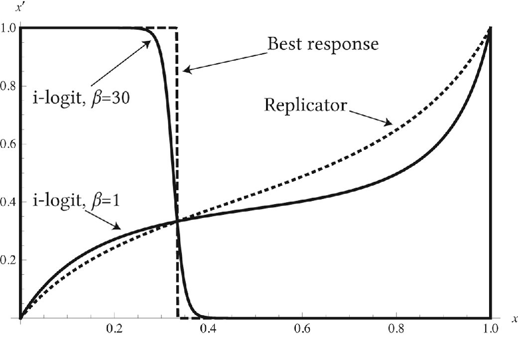
Consider fixing . Figure 1 shows the discrete-time i-logit dynamic with both and as well as the discrete-time replicator dynamic and the discrete-time best-response dynamic. It is easy to see that for low the discrete-time i-logit dynamic has behavior similar to that of the replicator dynamic, but for high the discrete-time i-logit dynamic has behavior similar to that of the best-response dynamic. This illustrates the fact that the parameterized i-logit family exhibits behaviors encompassing those seen in the low-rationality replicator dynamic and the highly rational myopic best-response dynamic.

Figure 1.

Discrete-time i-logit dynamic with and compared with the discrete-time replicator dynamic and the discrete-time best-response dynamic.

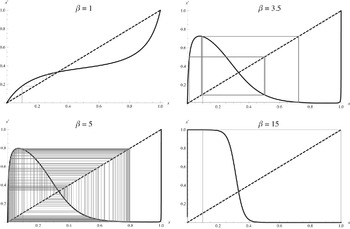
Figure 2 shows cobweb diagrams illustrating the long-term behavior of the discrete-time i-logit dynamic when for four different values of . All four diagrams show the evolution of the initial condition . When , the dynamic converges to the Nash equilibrium. This long-term behavior is identical to that of the discrete-time replicator dynamic. When , the dynamic converges to a cycle (of period 3) that has the population alternating between the majority playing each of the two strategies. This long-term behavior approximates that of the best-response dynamic. But for intermediate values of , the discrete-time i-logic dynamic exhibits more complicated behaviors. For example, when , the dynamic converges to a period 4 cycle, and when , it does not appear to converge to any sort of periodic behavior. Instead, the dynamic exhibits deterministic chaos.

Figure 2.

Cobweb diagrams showing the behavior of the i-logit dynamic with . All solution trajectories shown have the initial condition .

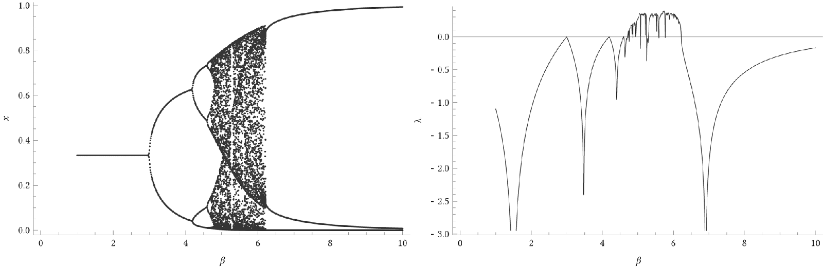
This chaos can be systematically investigated with orbit diagrams. These diagrams show the states that occur in the long run as the map is iterated. Figure 3 shows an orbit diagram for this system as increases from 1 to 10. This figure illustrates the period-doubling route to chaos typical of one-dimensional maps. It also shows the Lyapunov exponents for each value of in this range. Positive Lyapunov exponents indicate exponential divergence of nearby trajectories and are often considered the hallmark of chaotic dynamics.Footnote ⁵ For a one-dimensional map f, the Lyapunov exponent for an orbit starting at is

These exponents can be numerically computed using a scheme described in Strogatz (Reference Strogatz1994, 368–69). As figure 3 shows, the system has positive Lyapunov exponents for some values of , and thus the system does indeed exhibit deterministic chaos.

Figure 3.

Left, Orbit diagram showing the long-run behavior of the system; right, system’s Lyapunov exponent as is varied from 1 to 10.

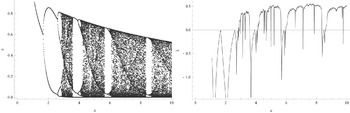
Figure 4 also shows an orbit diagram and Lyapunov exponents, but now with the payoff parameter a being varied. This parameter is the payoff that an agent using strategy 2 receives when she meets an agent using strategy 1. The game’s Nash equilibrium is located at , so as this parameter is increased, the equilibrium moves toward . When a is less than approximately 1.8, the dynamic converges to the Nash equilibrium. But if a is above this value, the dynamic does not lead to equilibrium play. It instead leads to either a periodic orbit or chaos.

Figure 4.

Left, Orbit diagram showing the long-run behavior of the system; right, system’s Lyapunov exponent as a is varied from 1 to 10 while .

4. Conclusion

The above is an example of a very simple game and a very simple process of imitative learning that yields a system that does not converge to the game’s sole equilibrium. This illustrates that a single-minded focus on static equilibrium concepts is perhaps misguided. Even in a game with just two strategies and just a single equilibrium, players may not converge to that equilibrium. And not only may players fail to converge, but the sequence of play may be chaotic and thus appear to be random.

It is sometimes claimed that nonconvergent dynamics are not realistic and are mere artifacts of unsophisticated learning rules. Real agents, the argument goes, are sophisticated enough to recognize and exploit out-of-equilibrium behavior, and this exploitation will drive the system to equilibrium. In their influential textbook on game-theoretic learning dynamics, Fudenberg and Levine sum up this sentiment as follows: “Our argument is that … when learning models fail to converge, the behavior of the model’s individuals is typically quite naive; for example, the players may ignore the fact that the model is locked in to a persistent cycle. We suspect that if the cycles persist long enough, the agents will eventually use more sophisticated inference rules that detect them; for this reason we are not convinced that models of cycles in learning are useful descriptions of actual behavior” (Reference Fudenberg and Levine1998, 3).

Much can be said about this argument. For one, the nonconvergent play exhibited by the system described above is not always cyclic; inside the chaotic regimes the behavior is aperiodic. Furthermore, the system’s sensitivity on initial conditions implies that it is impossible to make precise predictions about the system’s future state. Any slight error in measurement of the current state is magnified exponentially, and this makes exploitation of future behavior a tricky business.

But perhaps most important, it is not a lack of sophistication or rationality that leads to nonconvergence. When the myopic rationality parameter is low, the players are guaranteed to converge to the equilibrium, just like in the low-rationality replicator dynamic. Nonconvergence only occurs when is increased, and as grows players become more myopically rational. The quick speed at which rational agents adopt a best response causes the population to overshoot the equilibrium, so to speak. This overshooting is what creates periodic and chaotic attractors. If players are less likely to revise to a best response, then the population does not overshoot the equilibrium, and players converge to the equilibrium. Increasing does not endow the agents with any additional pattern matching or inferential abilities, but myopic rationality is one form of sophistication. And, contrary to what might be expected, increased rationality does not result in convergence to equilibriums. Instead, increased myopic rationality is the cause of the chaotic behavior, and the persistent out-of-equilibrium play, seen above.