1 Introduction
Safety in Artificial Intelligence (AI) has become an important focus of research as AI methods make rapid advancements (Amodei et al. Reference Amodei, Olah, Steinhardt, Christiano, Schulman and ManÉ2016). The 23 Asilomar AI principles (Future of Life Institute 2017) discuss a variety of safety aspects such as risk aversion, transparency, robustness, fairness, and also legal and ethical values that an agent must hold. In this work, we mainly focus on safety from the perspective of preventing undesirable behaviour, in particular, reducing visits to undesirable or risky states during the learning process of a reinforcement learning (RL) system.
RL algorithms optimize the expected value of cumulative rewards (return) obtained over time (Sutton & Barto Reference Sutton and Barto1998). For safety-critical applications such as finance, medicine, or industrial automation, optimizing the expected return alone is often not sufficient. An agent might exhibit undesirable behaviour over certain trajectories or for a certain period. In general, safety requires measuring some notion of risk or uncertainty in addition to maximizing the mean return thus ensuring that the learning algorithm also minimizes risk.
An additional challenge in RL is that agents need to explore during which an agent might be unaware of the states prone to noise or potentially leading to catastrophic consequences. Risk awareness in RL has been formulated in several ways, for example, by directed exploration that avoids the high entropy states (Law et al. Reference Law, Coggan, Precup and Ratitch2005), optimizing the worst-case performance instead of the expected performance of an agent (Tamar et al. Reference Tamar, Xu and Mannor2013), measuring and bounding the probabilities of visiting the erroneous states (Geibel & Wysotzki Reference Geibel and Wysotzki2005), and several other approaches. Garca and FernÁndez (Reference Garca and FernÁndez2015) present a comprehensive survey covering a broad range of techniques aimed at achieving safety in RL. In the context of Markov Decision Processes (MDPs), the source of uncertainty or variability in a sequential decision-making task can arise mainly from two sources—inherent stochastic uncertainty in the reward and the transition model (aleatoric uncertainty), and imperfect knowledge regarding the model (epistemic uncertainty). The former uncertainty is usually clustered under risk-sensitive MDPs (Howard & Matheson Reference Howard and Matheson1972; Heger Reference Heger1994; White Reference White1994; Borkar & Meyn Reference Borkar and Meyn2002), whereas the latter is covered under robust MDPs (Iyengar Reference Iyengar2005; Nilim & El Ghaoui Reference Nilim and El Ghaoui2005; Lim et al. Reference Lim, Xu and Mannor2013). In this work, we focus on risk-sensitive MDPs and address the former source of variability via mean-variance optimization.
The natural question that follows is how can we measure variance in RL? Several works focus on estimating the variance in return using temporal-difference (TD) style learning methods (Tamar et al. Reference Tamar, Di Castro and Mannor2012; Tamar et al. Reference Tamar, Di Castro and Mannor2016; Gehring & Precup Reference Gehring and Precup2013; Sherstan et al. Reference Sherstan, Ashley, Bennett, Young, White, White and Sutton2018; Jain et al. Reference Jain, Patil, Jain, Khetarpal and Precup2021). Our work is based on the specific approach proposed by Gehring and Precup (Reference Gehring and Precup2013), which suggests using the absolute value of the TD error to define controllability of a state. Intuitively, for an agent to exhibit safe behaviour, it will prefer taking the actions whose effects are more predictable on a state. Such states are referred as controllable. We redefine controllability slightly to provide an estimator which calculates the uncertainty in the value function and then show how to ‘encourage’ an agent to focus on controllable states. All approaches discussed so far define safety in the primitive action space (one-step action). Inspired by how humans think and plan, temporally abstract actions also provide a path to learn and plan efficiently. Temporal abstractions have been a crucial part of AI research since the 1970s (Fikes et al. Reference Fikes, Hart and Nilsson1972; Fikes et al. Reference Fikes, Hart and Nilsson1981; Iba Reference Iba1989; Korf Reference Korf1983; Parr & Russell Reference Parr and Russell1998; Sutton et al. Reference Sutton, Precup and Singh1999; Precup Reference Precup2000; Dietterich Reference Dietterich2000; McGovern & Barto Reference McGovern and Barto2001; Menache et al. Reference Menache, Mannor and Shimkin2002; Barto & Mahadevan Reference Barto and Mahadevan2003; Konidaris & Barto Reference Konidaris and Barto2007; Bacon et al. Reference Bacon, Harb and Precup2017; Barreto et al. Reference Barreto, Borsa, Hou, Comanici, AygÜn, Hamel, Toyama, Mourad, Silver and Precup2019). Prior research has shown that the temporal abstractions can improve exploration, reduce the complexity of deliberation, and enhance robustness. More importantly, from the safety perspective, temporal abstractions lead to composition of behaviour and predictions. To simplify, if every subpart of the abstraction hierarchy can be derived respecting the safety conditions, the entire hierarchy would automatically be safe in behaviour. In this paper, we take the first step in this direction by showing how to construct temporally safe extended actions by reducing the variability or uncertainty as discussed above.
We approach this problem in the options framework (Sutton et al. Reference Sutton, Precup and Singh1999; Precup Reference Precup2000), which provides an intuitive way to plan, reason, and act at multiple timescales. We are especially interested in learning options end-to-end from the data obtained by the agent’s interaction with the environment. The options framework has received a lot of attention over time, for example, Stolle and Precup (Reference Stolle and Precup2002), Konidaris and Barto (Reference Konidaris and Barto2007), Konidaris et al. (Reference Konidaris, Kuindersma, Grupen and Barto2011); Daniel et al. (Reference Daniel, Van Hoof, Peters and Neumann2016); Kulkarni et al. (Reference Kulkarni, Narasimhan, Saeedi and Tenenbaum2016); Vezhnevets et al. (Reference Vezhnevets, Mnih, Osindero, Graves, Vinyals and Agapiou2016); Mankowitz et al. (Reference Mankowitz, Mann and Mannor2016), Jain and Precup (Reference Jain and Precup2018), Riemer et al. (Reference Riemer, Liu and Tesauro2018); Barreto et al. (Reference Barreto, Borsa, Hou, Comanici, AygÜn, Hamel, Toyama, Mourad, Silver and Precup2019).
Bacon et al. (Reference Bacon, Harb and Precup2017) introduced the option-critic framework by adapting to the actor-critic model. The option-critic model facilitates an end-to-end learning of options without the need to specify sub-goals. We modify the option-critic objective to include the negation of controllability (Gehring & Precup Reference Gehring and Precup2013) (estimates the variability in the performance) as a regularizer in the optimization objective. Consequently, the key contributions of this work can be summarized as follows:
-
1. We propose a new objective function which uses the effect of the uncertainty in the return as a regularizer for the classical optimization problem of maximizing the expected return. We then use this objective to derive a policy gradient algorithm for automatically learning safe options.
-
2. We empirically demonstrate the effectiveness of our approach in the tabular setup.
-
3. We also show that our method is scalable to both linear and non-linear function approximation settings using the puddle world and ALE games: Ms. Pacman, Amidar, and Q*Bert.
The paper is structured as follows. After presenting definitions and notations in Section 2, we introduce the safe option-critic algorithm in Section 3. Next, we present tabular, continuous, and ALE experiments in Section 4. Finally, we conclude with discussion and future work in Section 5.
2 Preliminaries
In RL, an agent interacts with the environment at discrete time steps
 $t \in \{1,2,...\}$
. At each step, the agent observes a state
 $s \in \mathcal{S}$
and chooses an action
 $a \in \mathcal{A}$
according to a policy which defines a probability distribution of actions over the state space
 $\pi: \mathcal{S} \times \mathcal{A} \to [0,1]$
. Afterwards, the agent transitions from
 $S_t$
to
 $S_{t+1}$
state according to the transition probability distribution
 $P:\mathcal{S} \times \mathcal{A} \times \mathcal{S} \to [0,1]$
. After transitioning to a next state, an agent receives a reward
 $R_{t+1} \in \mathbb{R}$
, where the expected reward function is
 $r(s,a)= \sum_{r\in \mathbb{R}}r \sum_{s'}P(s',r|s,a)$
, and
 $r: \mathcal{S} \times \mathcal{A} \to \mathbb{R}$
. The MDP is defined as a tuple of
 $(\mathcal{S}, \mathcal{A}, r, P, \gamma)$
, where
 $\gamma \in [0,1]$
is the discount factor, which de-values rewards received farther into the future. A MDP with the defined optimality criteria is known as a Markov Decision Problem. In this work, we focus on MDP with optimality criteria as the expected total discounted reward. According to these optimality criteria, we define the state-action value function as
 $Q(s,a) = \mathbb{E}_\pi[ \sum_{t=0}^{\infty} \gamma^t R_{t+1}|S_t = s, A_t = a]$
. An estimate of Q can be learned in an incremental fashion using TD learning methods (Sutton, Reference Sutton1988). For example, in TD(0), the agent computes a TD error, which captures the difference in the agent’s value estimate at two consecutive time steps:
 \begin{equation*}\delta_t = R_{t+1} + \gamma Q(S_{t+1}, A_{t+1}) - Q(S_t, A_t).\end{equation*}
The state-action value function is then updated as:
 \begin{equation*}Q(S_{t}, A_t) \gets Q(S_t,A_t) + \alpha \delta_t,\end{equation*}
where
 $\alpha\in [0,1]$
is the step size.
The policy gradient theorem (Sutton et al. Reference Sutton, McAllester, Singh and Mansour2000) provides a way to update a parameterized policy in the direction of the gradient of the expected return. Here, return is the total discounted rewards received in a trajectory. The performance of a policy
 $\pi$
is measured by the expected return as
 \begin{equation*}\rho(\pi, s_0) = \mathbb{E}[\sum_{t=0}^{\infty}\gamma^{t} R_{t+1}| \pi, s_0],\end{equation*}
where the initial state is denoted by
 $s_0$
. The gradient of the performance with respect to the policy parameter
 $\theta$
is given by:
 \begin{equation} \frac{\partial \rho(\pi, s_0)}{\partial \theta} = \sum_{s} d^\pi (s|s_0) \sum_{a} \frac{\partial \pi(s,a)}{\partial \theta} Q_\pi(s,a),\end{equation}
where
 $d^\pi(s|s_0) = \sum_{t=0}^{\infty} \gamma^t \it{P(S_t = s | s_0, \pi)}$
is the discounted weighting of the states.
2.1 Options
The options framework (Sutton et al. Reference Sutton, Precup and Singh1999; Precup Reference Precup2000) facilitates the incorporation of temporally abstract knowledge into RL. An option
 $w\in \mathcal{W}$
is defined as a tuple of
 $(I_w, \pi_w, \beta_w)$
.
 $I_w$
is an initiation set containing initial states from which an option w can start.
 $\pi_w$
denotes an option policy that defines a distribution over actions given a state during the execution of option w. The termination condition of w option,
 $\beta_w$
, defines a probability of termination in each state.
If the option policies are Markovian, the intra-option Bellman equation (Sutton et al. Reference Sutton, Precup and Singh1999) provides an off-policy method for updating the value of a state-option pair as
 \begin{align*} Q(S_t,W_t) \gets Q(S_t, W_t) + \alpha \Big(&R_{t+1} +\gamma(1-\beta_{W_t}(S_{t+1}))Q(S_{t+1}, W_t) \\ &+\gamma \beta_{W_t}(S_{t+1})\max_{w' \in \mathcal{W}} Q(S_{t+1}, w') - Q(S_t, W_t)\Big),\end{align*}
where the same option w continues with
 $1-\beta_w$
probability, or terminates with
 $\beta_w$
probability and selects the next best option.
2.2 Option-critic architecture
The above described intra-option value learning (Sutton et al. Reference Sutton, Precup and Singh1999) also lays the foundation for how the options are learnt in the Option-Critic architecture (Bacon et al. Reference Bacon, Harb and Precup2017). The option-critic method is a policy gradient-based method for learning intra-options policies and option’s termination conditions. Bacon et al. (Reference Bacon, Harb and Precup2017) consider the call-and-return option execution model, where an option w is chosen according to a policy over options
 $\pi_{W}$
, and an intra-option policy
 $\pi_w$
is followed until the termination condition
 $\beta_w$
is met. Once the current option terminates, another option is selected using
 $\pi_{W}$
and the process continues. Let
 $\pi_{w, \theta}$
denotes intra-option policy parameterized by
 $\theta$
, and
 $\beta_{w, \nu}$
represents the option termination parameterized by
 $\nu$
. The value of executing an action a at a particular state-option pair is given by
 $Q_U: \mathcal{S} \times \mathcal{W} \times \mathcal{A} \to \mathbb{R}$
which is defined as
 \begin{equation}Q_U(s, w, a) = r(s, a) + \gamma \, \sum_{s'} P(s'| s, a) U(s',w),\end{equation}
where U(s’,w) represents the value of arriving through an option w at a state s’. Here, either the option w could terminate with
 $\beta_{w, \nu}$
probability and select the other options, or could continue with the same option with
 $(1- \beta_{w, \nu})$
probability,
 \begin{equation}U(s',w) = (1 - \beta_{w, v} (s')) Q_{W}(s', w)\, +\, \beta_{w, v} (s') V_W(s').\end{equation}
Here,
 $Q_W$
represents the value function over options, which is given by-
 \begin{equation*}Q_W(s,w) = \sum_a \pi_{w, \theta}(a|s) Q_{U}(s,w, a).\end{equation*}
 $V_W$
represents the value function of executing policy over options
 $\pi_W$
, given by-
 \begin{equation*}V_W(s) = \sum_w\pi_W(w|s) Q_{W}(s, w).\end{equation*}
Bacon et al. (Reference Bacon, Harb and Precup2017) derived the gradient of the discounted return from an initial condition
 $(s_0, w_0) \in (\mathcal{S \times W})$
with respect to
 $\theta$
(intra-option policy parameter) as:
 \begin{align} \frac{\partial \rho(\pi, s_0, w_0)}{\partial \theta} =&\sum_{s,w} \mu(s, w| s_0, w_0) \sum_{a} \frac{\partial \pi_{w, \theta}(a | s)}{\partial \theta} Q_U(s, w, a),\end{align}
where
 $\mu(s, w| s_0, w_0) = \sum_{t=0}^{\infty} \gamma^t P(S_t=s,W_t=w|s_0,w_0)$
is the discounted weighting of a state-option pair. The gradient of the expected discounted return with respect to the option termination parameter
 $\nu$
and the initial condition
 $(s_1, w_0)$
is given by:
 \begin{equation}\frac{\partial \rho(\pi, s_1, w_0)}{\partial v}=-\sum_{s',w} \mu(s', w|s_1, w_0)\frac{\partial \beta_{w, \nu}(s')}{\partial \nu} A_W(s', w),\end{equation}
where
 $A_W$
is the advantage function
 $A_W(s,w) = Q_W(s,w) - V_W(s)$
. In (5), the initial condition changed from
 $(s_0,w_0)$
to
 $(s_1, w_0)$
because given an initial state-option
 $(s_0, w_0)$
, the first action is selected according to
 $\pi_{w_0}$
policy, and then the agent transitions to the next state
 $s_1$
. The updates to the termination parameter
 $\nu$
are made thereafter based on the advantage of switching to the next option in state s’.
3 Safe option-critic model
In this work, we introduce a notion of learning safe hierarchical policies using a penalty based on the variance in TD error. Previous works in the literature had focused on the measures derived from the TD-based methods for quantifying uncertainty in the value of a state or a state-action pair.
As mentioned earlier, here, we focus on addressing uncertainty arising due to inherent stochasticity present in the model (aleatoric uncertainty). The uncertainty present in the model is reflected in the form of variability in the value function. One such feasible approach to capture the uncertainty/variability in the value function would be to estimate the variance in TD error. After the policy has converged, the expected TD error would approach zero value. The variance in the TD error results from the stochasticity in the environment’s reward function and the transition dynamics. We define ‘safety’ as constraining the uncertainty in the value function. Therefore, we modify the objective function of maximizing the mean return by adding a regularizer on uncertainty in the value function.
Inspired by Gehring and Precup (Reference Gehring and Precup2013), we define controllability as a negation of the variance in TD error of a state-option action pair. We use the aforementioned definition of controllability to introduce the concept of safety in the option-critic architecture, which aids in measuring the uncertainty in the value of a state-option pair. The key idea is—the higher the variance in TD error of a state-option pair, the higher would be the uncertainty in the value function.
In safety-critical applications, the agent must learn to avoid such state-option pairs as they induce variability in return eventually. We optimize for obtaining the maximum expected discounted return and controllability value of the initial state-option pair. Depending on the nature of the application, one can limit or encourage the agent’s visit to a state-option pair based on the degree of controllability. Introducing controllability via the TD error facilitates the linear scalability of the proposed approach with the number of state-option pairs.
Analogous to the notations used in Bacon et al. (Reference Bacon, Harb and Precup2017), we introduce a parameter vector described by
 $\Theta = [\theta, \nu]$
, where
 $\theta$
is an intra-option policy parameter and
 $\nu$
is an option termination parameter. We assume that all options can be initialized from any state such that
 $I_w= \mathcal{S}, \, \forall w\in \mathcal{W}$
. Uncertainty in the value of a state-option pair is measured using controllability C, which is given by the negation of the variance in the TD error
 $(\delta)$
. The TD error is
 \begin{equation}\delta(S_t, W_t, A_t) = R_{t+1} \, + \gamma \sum_{s'} P(s' | S_t, A_t) U_\Theta(s',W_t) - Q_{U,\Theta}(S_t, W_t, A_t),\end{equation}
where
 $Q_{U,\Theta}(s,w,a)$
and
 $U_\Theta(s, w)$
are defined in (2) and (3), respectively. For the ease of notation, we will use
 $\delta_t$
to denote
 $\delta(S_t, W_t, A_t)$
. Whenever it is not clear from the context, we will use the full notation for the TD error. The expected value of the TD error would converge to zero. Therefore, the variance in TD error can be simplified to denote controllability as:
 \begin{align}C_{\Theta}(s, w) &= - Var_{\pi_{w,\theta}}[\delta_t | S_t=s, W_t= w]\nonumber\\[3pt]&= - \Big(\mathbb{E}_{\pi_{w,\theta}}\big[\delta_t^2 | S_t=s, W_t= w\big] - \mathbb{E}_{\pi_{w,\theta}}\big[\delta_t | S_t=s, W_t= w\big]^2\Big)\nonumber\\[3pt]&= -\mathbb{E}_{\pi_{w,\theta}}\big[\delta_t^2 | S_t=s, W_t= w\big].\end{align}
The aim here is to maximize both the expected discounted return and the controllability value from an initial state-option pair. We want to maximize the objective function J,
 \begin{align}&\max_\Theta J(\Theta | \kappa),\nonumber\\[3pt] &\text{where }\, J(\Theta | \kappa) = \mathbb{E}_{(s_0, w_0) \sim \kappa}\Big[Q_\Theta(s_0, w_0) + \psi\, C_\Theta(s_0, w_0)\Big],\end{align}
 $\psi \in \mathbb{R}$
is a regularizer on the controllability value, and
 $\kappa$
denotes the initial state-option pair distribution. The value of a state-option pair is defined as
 $Q_\Theta(s, w) = \sum_{a} \pi_{w, \theta} (a | s)\, Q_{U, \Theta}(s, w, a)$
. Another interpretation is to view the above objective as a constrained optimization problem, where the constraints are imposed on the controllability function. One could bound the controllability value, but it would require specific assumptions about the environment or one needs to rely on an input value from the user. In this paper, we opted to keep the method general without the need to rely on certain assumptions regarding the environment. We will now derive the gradient of the performance evaluator J with respect to the intra-option policy parameter
 $\theta$
, assuming that they are differentiable.
First, we calculate the gradient of the
 $\delta_t$
with
 $\theta$
using (6):
 \begin{align} \frac{\partial \delta_t}{\partial \theta} &= \gamma \sum_{s'} P(s'| S_t, A_t)\frac{\partial U_\Theta(s', W_t)}{\partial \theta} - \frac{\partial Q_{U, \Theta}(S_t, W_t, A_t)}{\partial \theta}\nonumber\\ &= \gamma \sum_{s'} P(s'| S_t, A_t)\frac{\partial U_\Theta(s', W_t)}{\partial \theta} - \Big(\gamma \sum_{s'} P(s'| S_t, A_t)\frac{\partial U_\Theta(s', W_t)}{\partial \theta}\Big)\nonumber\\[3pt] &=0\end{align}
The above equation follows through (2). Next, we take the gradient of C with respect to
 $\theta$
. Following from (7),
 \begin{align}\frac{\partial C_\Theta(s_0, w_0)}{\partial \theta} &= -\frac{\partial \{\sum_a \pi_{w_0, \theta}(a | s_0) \delta(s_0, w_0, a)^2\}}{\partial \theta}\nonumber\\ &=-\sum_{a}\frac{\partial \pi_{w_0, \theta}(a | s_0)}{\partial \theta}\, \delta(s_0, w_0, a)^2 -\, 2\sum_{a}\pi_{w_0, \theta}(a | s_0) \delta(s_0, w_0, a) \frac{\partial \delta(s_0, w_0, a)}{\partial \theta}\nonumber\\&=-\sum_{a}\frac{\partial \pi_{w_0, \theta}(a | s_0)}{\partial \theta}\, \delta(s_0, w_0, a)^2 \qquad\text{[Using (\ref{eqn9})]}\end{align}
The last term in the above equation vanishes because the gradient of TD error with respect to the policy parameter
 $\theta$
is zero (using (9)).
The one-step state-option transition is denoted by
 \begin{equation*}P_{\gamma}^{(1)}(s', w' | s, w) = \gamma\sum_{a}\pi_{w,\theta}(a|s)P(s'|s, a)\big[\, (1-\beta_{w,\nu}(s'))\mathbb{1}_{w= w'} + \beta_{w,\nu}(s')\pi_W(w' | s')\big].\end{equation*}
Using the above one-step transition, similarly, the k-step state-option transition is expressed as
 \begin{equation*}P_{\gamma}^{(k)}(s', w' | s_0, w_0) = P_{\gamma}^{(1)}(s_1, w_1 | s_0, w_0) \times P_{\gamma}^{(k-1)}(s', w' | s_1, w_1).\end{equation*}
Using the Intra-Option Policy Gradient Theorem (Bacon et al. Reference Bacon, Harb and Precup2017), the gradient of
 $Q_\Theta(s,w)$
with
 $\theta$
is:
 \begin{align}\frac{\partial Q_\Theta(s_0,w_0)}{\partial \theta} = \sum_{k=0}^{\infty} \sum_{s',w'}P_{\gamma}^{(k)}(s',w' | s_0,w_0) \sum_{a} \frac{\partial \pi_{w', \theta}(a | s')}{\partial \theta} Q_{U, \Theta}(s',w', a).\end{align}
Following the objective function (8), combining the gradient of
 $Q_\Theta(s_0,w_0)$
(11) and
 $C_\Theta(s_0,w_0)$
(10), the gradient of J with
 $\theta$
is:
 \begin{align} \frac{\partial J(\Theta| \kappa)}{\partial \theta} =& \sum_{k=0}^{\infty}\sum_{s, w} \Big\{P_\gamma^{(k)} (s, w| s_0, w_0) \sum_{a} \frac{\partial \pi_{w, \theta}(a |s)}{\partial \theta} Q_{U, \Theta}(s, w, a) \Big\} \nonumber\\& - \psi\sum_{a} \frac{\partial \pi_{w_0, \theta}(a |s_0)}{\partial \theta} \delta(s_0,w_0,a)^2.\end{align}
In (12),
 $(s_0,w_0)$
corresponds to the initial state-option pair. In the above equation, one can simply replace
 $Q_{U, \Theta}(s, w, a)$
with the advantage term
 $A_{\Theta}(s,w,a) = Q_{U, \Theta}(s, w, a) - Q_{\Theta}(s,w)$
because,
 \begin{equation}\sum_{a} \frac{\partial \pi_{w, \theta}(a |s)}{\partial \theta} Q_{\Theta}(s,w) = Q_{\Theta}(s,w) \frac{\partial \sum_{a} \pi_{w, \theta}(a |s)}{\partial \theta} = Q_{\Theta}(s,w) \frac{\partial 1}{\partial \theta} = 0.\end{equation}
The gradient update of J here describes that each option aims to maximize its own reward, along with, maintaining a high controllability value pertaining to that option policy only.
Now, we will compute the gradient of
 $J(\Theta | \kappa)$
with respect to the option termination function parameter
 $\nu$
. First, we would calculate the gradient of TD error with
 $\nu$
.
 \begin{align} \frac{\partial \delta_t}{\partial v} =& \gamma \sum_{s'} P(s' | S_t, A_t) \frac{\partial U_\Theta(s', W_t)}{\partial \nu} - \frac{\partial Q_{U,\Theta}(S_t, W_t, A_t)}{\partial \nu} \nonumber\\ &=\gamma \sum_{s'} P(s' | S_t, A_t) \frac{\partial U_\Theta(s', W_t)}{\partial \nu} - \Big(\gamma \sum_{s'} P(s' | S_t, A_t) \frac{\partial U_\Theta(s', W_t)}{\partial \nu} \Big)\nonumber\\ &=0 \end{align}
The last equation follows through (2). The gradient of controllability C with
 $\nu$
using (7) and (14) can be expressed as:
 \begin{align}\frac{\partial C_\Theta(s_0, w_0)}{\partial \nu} &= - \sum_a \pi_{w_0, \theta}(a | s_0)\frac{\partial \delta(s_0, w_0, a)^2}{\partial \nu}\nonumber\\ &=-2 \sum_{a} \pi_{w_0, \theta}(a | s_0)\, \delta(s_0, w_0, a) \frac{\partial \delta(s_0, w_0, a)}{\partial \nu}\nonumber\\ &= 0 \qquad \text{[Using (\ref{eqn14})]}\end{align}
Therefore, the gradient of J with
 $\nu$
remains same as the gradient of the state-option value. On using the Termination Gradient Theorem (Bacon et al. Reference Bacon, Harb and Precup2017), the gradient of J with
 $\nu$
results as follows:
 \begin{align}\frac{\partial J(\Theta| \kappa)}{\partial \nu} &= \frac{\partial Q_\Theta(s_1, w_0)}{\partial \nu} \nonumber\\&= - \sum_{k=0}^{\infty}\sum_{s, w} P_\gamma^{(k)} (s, w| s_1, w_0) \frac{\partial \beta_{w,\nu}(s)}{\partial \theta} A_{W}(s, w).\end{align}
Our interpretation of the above derivation follows the notion of safety; each option is responsible for making its intra-option policy safe by incorporating the controllability function. Due to the assumption that each option takes care of its own safety through the intra-option policy (the objective function implicitly does not bring changes at the policy over options level), one is only concerned about choosing an option that maximizes the expected discounted return from the next state-option pair while terminating an option. As a result, introduction of controllability does not impact the termination function update. Algorithm 1 shows a prototype implementation details of controllability in the option-critic architecture in the look-up table setting.
We now provide some intuition behind using the variance of TD error to learn the controllable states. The variance in the TD error of the initial state-option-action
 $\delta(s_0,w_0, a_0)$
uses the difference in the current state-option value
 $Q_{U,\Theta}(S_t, W_t, A_t)$
and the next expected state-option value
 $\mathbb{E}[U_{\Theta}(s', W_t)| S_t =s]$
. With the increase in the time steps, the estimate of the Q value function changes (on seeing the new reward samples along a trajectory, the Q function estimate changes). Therefore, the square of the TD error would capture the variations in the return (sum of rewards) from the initial state-option pair onwards, thus yielding the uncertainty in the value function estimates.

4 Experiments
4.1 Grid world
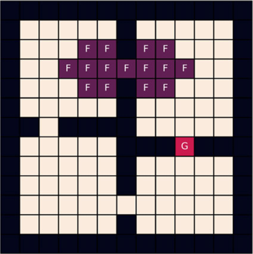
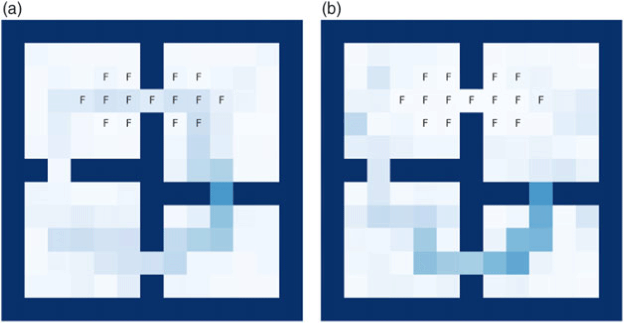
First, we consider a simple navigation task in a two-dimensional grid environment using a variant of the four-room domain as described in Sutton et al. (Reference Sutton, Precup and Singh1999). As shown in Figure 1, similar to Gehring and Precup (Reference Gehring and Precup2013), we define some slippery frozen states in the environment which are unsafe to visit. We accomplish this by introducing variability in the rewards of these frozen states. The states labelled as F and G indicate the frozen and the goal states, respectively.
Four-Room (FR) environment: F and G depict the unsafe frozen and goal states, respectively. The lightest colour represents the normal states, whereas the darkest colour represents the wall.

An agent can be initialized with any random start state in the environment apart from the goal state. The action space consists of four stochastic actions, namely, up, down, left, and right. Upon choosing an action, with
 $0.2$
probability, the agent can transition into any of the four directions (irrespective of the selected action), whereas, with
 $0.8$
probability, an agent takes the intended action deterministically. The task is to navigate through the rooms to a fixed goal state as depicted in Figure 1. The dark states in Figure 1 depict the walls. The agent remains in the same state with a reward of 0 if the agent hits the wall. A reward of 0 and 50 is given to the agent on transitioning into the normal and the goal state, respectively. Rewards for the unsafe states are drawn from
 $\mathcal{N}(\mu=0, \sigma = 15)$
distribution when the agent transitions to a slippery state. The expected value of the reward for the normal and the slippery states is the same.
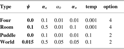
Here, we are using a look-up table representation to learn the policy. In the safe option-critic framework, we represent both policy over options and intra-option policies with the Boltzmann distribution. Sigmoid activation is used for learning the termination function. We ran the experiments with different controllability factor
 $\psi$
for learning four options. One could choose a different number of options as well. We optimize for the hyperparameters: temperature and step size for both the baseline Option-Critic (OC) with
 $\psi=0$
and Safe-OC. The discount factor
 $\gamma$
is set to
 $0.99$
. Hyperparameters for the experiment are mentioned in Table 1. We ran the experiments for a total of 500 episodes averaged over 50 trials, where the training in each trial starts from scratch. In each episode, the agent is allowed to take a maximum of only 500 steps, wherein if the agent fails to reach the goal state within those steps, then the episode terminates.
Parameters for discrete and continuous environment: Optimized parameters for both four-room and puddle-world environments

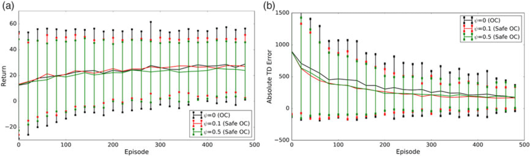
Performance in the FR domain. The graphs depict the performance averaged over 50 independent trials, where the vertical bands depict the standard deviation. The plots show (a) the return and (b) the sum of absolute TD error. Safe policy
 $\psi=0.1$
(red) has a smaller standard deviation as compared to the baseline (black) signifying that safety helps the agent to avoid the variance inducing regions.

To evaluate these experiments, we consider the following metrics: compared the expectation and the variance in the performance over multiple trials (to comment on the stability of the introduced algorithm); sum of the absolute TD error over episodes; and density of the state visits. We also show sampled trajectories from both the baseline and the proposed method to qualitatively express the differences between the two after learning has been completed.
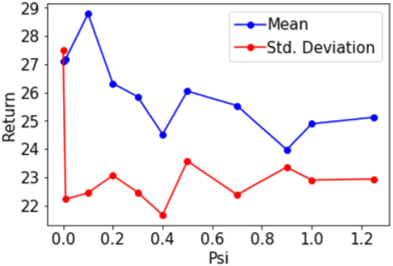
It can be observed from Figure 2a that the options with the controllability (Safe-OC) have a lower standard deviation in the return of an episode as compared to the baseline, that is, options without any notion of safety (OC). Figure 2b represents a lower standard deviation in the absolute sum of the TD error with safety. This highlights the fact that the controllability helps the agent to avoid the unsafe states (variable reward), thus resulting into a smaller variance in the sum of absolute TD error over multiple trials. Figure 3 shows how the performance (expectation and variance in the return) varies with the change in the controllability regularizer
 $\psi$
. We chose the optimal value of
 $\psi$
which not only maximizes the mean but also minimizes the variance in return. From the figure, it can be easily seen that
 $\psi=0.1$
leads to not only maximum expectation but also significant reduction in the variance of return. We also visualize the state frequency graph depicted in Figure 4. It is observed that the options with the controllability function have lower frequency of visit to the frozen states (risky) as opposed to the vanilla options.
Performance with varying variance regularizer in Four-Room (FR) domain. The plot shows the mean and standard deviation of the score in the FR domain with varying controllability regularizer value
 $\psi$
, while keeping all other parameters fixed. The best hyperparameters are chosen such that they not only minimize the standard deviation but also maximize the mean performance, which in this case is achieved by
 $\psi=0.1$
.

State visitation frequency in Four-Room environment. Density graph represents the number of times a state was visited during testing over 80 independent trials. Darker shades of blue represent a higher density. (a) Model without safety has equally likely density for both the hallways. (b) Model with safety shows higher density for the path without the frozen states.

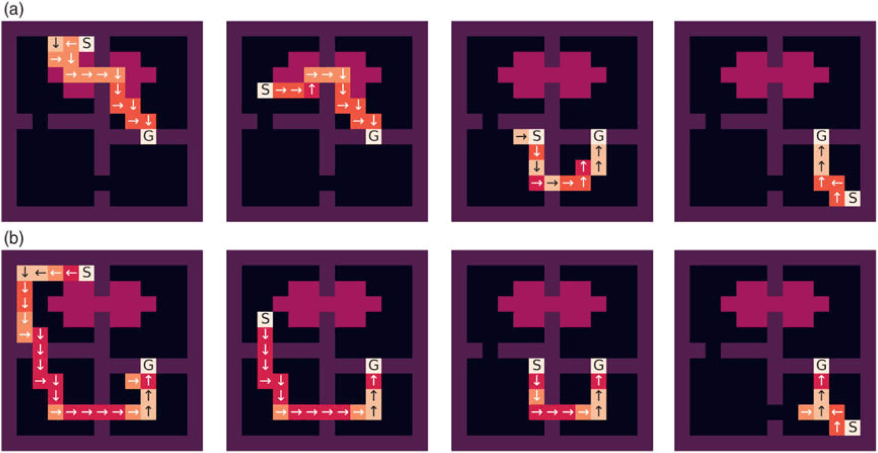
Learning of safe options induces transparency in the behaviour of an agent. This is most explicitly demonstrated through the trajectory taken by the agent without controllability regularizer (baseline OC) and with controllability regularizer (Safe-OC) as shown in Figure 5. Regardless of the start state, Safe-OC agent navigates to the goal state by avoiding the states with a high variance in the reward, as opposed to the OC agent, which finds a shortest route to the goal state being unaware of the risky states.
Policy in Four-Room (FR) environment. Sampled trajectories learned with 4 options where S and G represent the start & goal state, respectively. Arrows denote the 4 actions. Agent might take different actions due to environment stochasticity. Change in colour represents the option switching. Same colour represents the same option choice. Purple patch represents the frozen states. (a) depicts the policy with
 $\psi=0$
passing through the frozen area. (b) depicts the policy learned with
 $\psi=0.1$
that avoids the frozen area due to the in-built safety constraint.

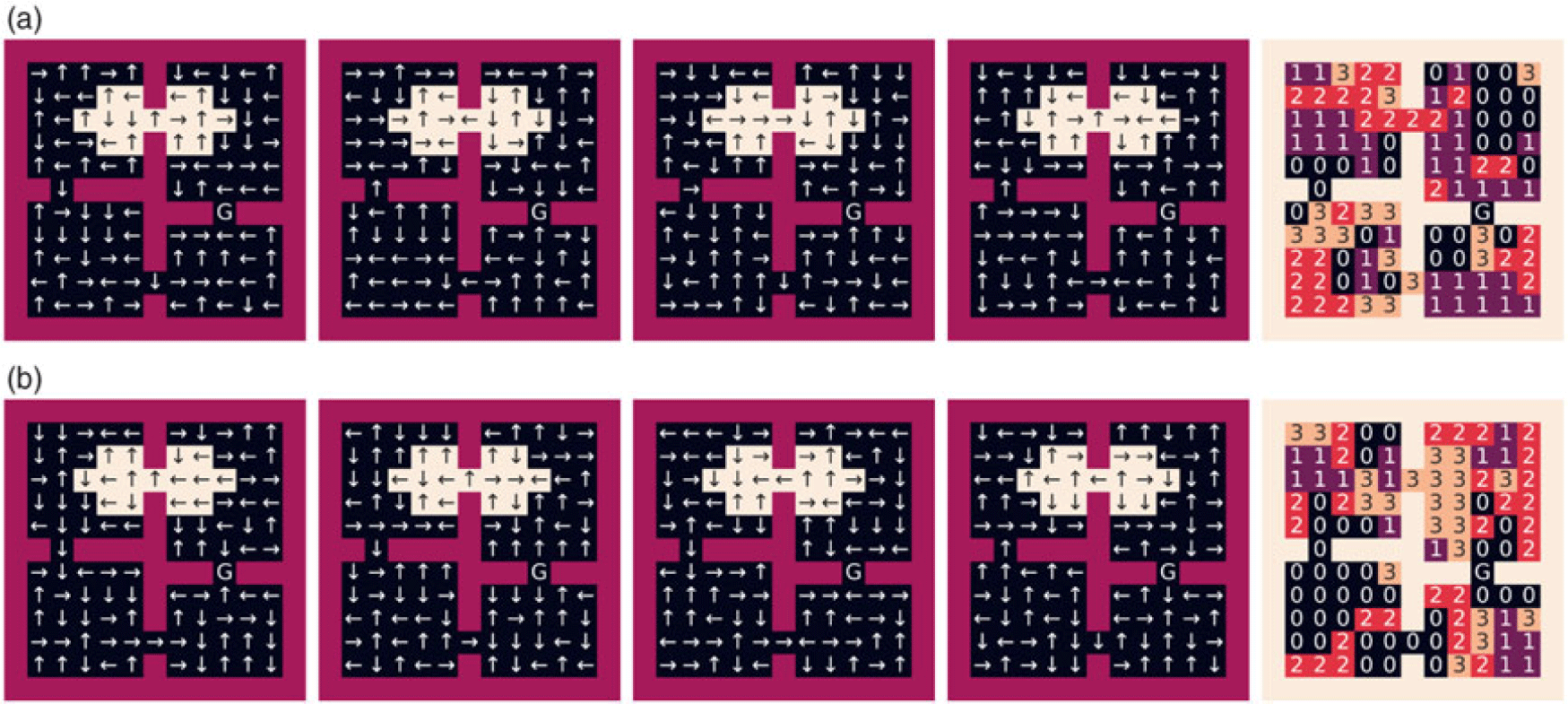
To capture how each option is behaving, we plotted the converged policy for all the options in Figure 6. It can be observed that each option does not capture the safety for the entire state space, but rather a subset of state space. The switches among the options for the safety are similar to the baseline (last image in both the rows). The overall trend observed from the individual option policy of safe algorithm is to avoid the unsafe frozen patch, whereas the vanilla option policies do not differentiate between the two hallways.
Converged policy for four options in Four-Room environment. The first four figures in each row depict the intra-option policy for all the four options. The last figure in both the rows shows the policy over the options where the number depicts the different options (numbering of options increases from left to right image in a row). Both the baseline and the Safe OC exhibit that the overall hierarchical policy is more reasonable than the individual option policy, though the overall trend of an individual safe option policy is to avoid the frozen hallway.

4.2 Continuous state-space environment
In this section, we examine the performance in the puddle-world Open AI gym environment with the linear function approximation. It is a continuous two-dimensional state-space environment in
 $[0,1]^2$
. The action space consists of four actions that change the position by a value of
 $0.05$
in any one of the coordinates. In each transition, noise is drawn from the
 $\textit{Uniform}[-0.025, 0.025]$
distribution, which is added to both the coordinates. For introducing the notion of unsafe regions, similar to the four-room environment, we added a square puddle region with a centre at
 $(0.5, 0.5)$
and
 $0.4$
height. An agent can be randomly initialized from any state, and the goal is located at (1,1). When the agent is within
 $0.1$
L1 distance from the goal state, the agent receives a reward of 50. Whenever the agent transitions from a puddle region, it receives a reward from a normal distribution of
 $\mathcal{N}(\mu=0, \sigma=8)$
, and 0 reward otherwise. On expectation, the reward received from both regions is the same. The penalty makes the puddle locations ‘unsafe’ due to the variability in the rewards.
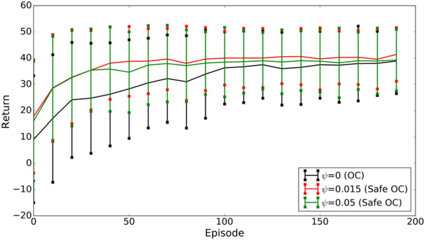
Puddle-world environment: The graphs depict the return averaged over 50 independent trials with 2 options. The vertical bands show the standard deviation in the return over multiple trials. The experiment with safe policy
 $\psi=0.015$
(red) has a smaller standard deviation as compared to the baseline (black), signifying safety helps an agent to avoid variance inducing regions.

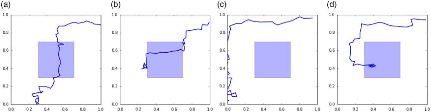
Trajectories in Puddle World: The graph shows sampled trajectories from OC policy in (a) & (b), and Safe-OC policy in (c) & (d). With the designed safety constraint, the agent learns to bypass the unsafe central puddle.

For these experiments, we use two options. One could choose to have more number of options, but given the complexity of the task, we decide to use only two options. We use intra-option Q-learning in the critic to learn policy over options. Boltzmann distribution is used to represent both intra-option policies and policy over options with a temperature value of
 $0.1$
. To learn the termination function, we use sigmoid activation. The agent can take a maximum of 5000 steps in an episode. The standard tile coding (Sutton & Barto Reference Sutton and Barto1998) is used for discretizing the state-space. We use 5 tilings, each of
 $5 \times 5$
over the joint space of two features which is hashed to a vector of 1024 dimension. The discount factor
 $\gamma$
is set to
 $0.99$
. The optimized parameters are shown in Table 1. The code for both the discrete four-rooms and the continuous puddle world is available at Github
Footnote 1
.
Figure 7 shows the return observed in the puddle-world domain with different values of
 $\psi$
averaged over 50 trials. The best performance in terms of stability was observed by
 $\psi=0.015$
Safe-OC which exhibits a reduction in the standard deviation of the return across multiple runs as compared to the baseline (
 $\psi=0$
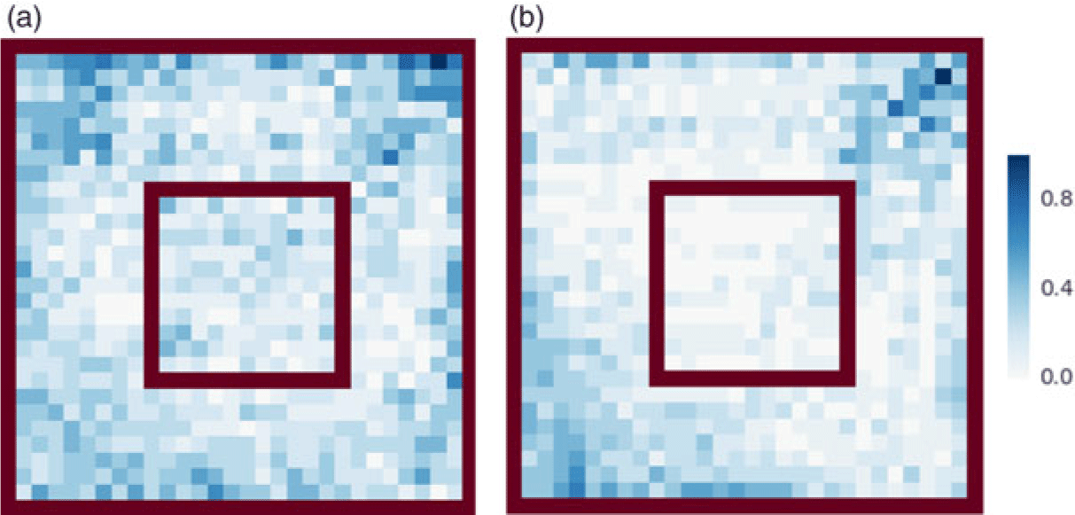
). This highlights that the agent following the safe policy learns to avoid the variance inducing puddle region. Figure 8 shows the sampled trajectories from both the baseline OC and the Safe-OC. To further validate, the frequency of visits is shown in Figure 9a and 9b. They describe the average number of visits across multiple runs for an episode, depicting a decrease in the number of visits to the unsafe puddle region in the safe policy learning option-critic framework as compared to the baseline. It demonstrates that the safe policy learning agent avoids the erratically behaving unsafe puddle region placed at the centre of the state space.
Visitation frequency in Puddle-World environment depicts the state visitation frequency averaged over 50 independent trials for a particular episode in the (a) baseline OC and (b) Safe-OC. The graph highlights that the Safe-OC agent’s visit to the unsafe central puddle region decreases in comparison to the OC agent. Our notion of safety enforces the agent to avoid the puddle region.

4.3 Arcade learning environment
We now analyze our method in the ALE domain (Bellemare et al. Reference Bellemare, Naddaf, Veness and Bowling2013). Harb et al. (Reference Harb, Bacon, Klissarov and Precup2018) introduced deliberation cost in the options framework to learn temporally extended options by adding a penalty cost on switching options too frequently. We use the asynchronous advantage option-critic (A2OC) (Harb et al. Reference Harb, Bacon, Klissarov and Precup2018) as our baseline for learning ‘safe’ options with non-linear function approximation. A2OC provides an extension of the asynchronous advantage actor-critic (A3C) algorithm (Mnih et al. Reference Mnih, Badia, Mirza, Graves, Lillicrap, Harley, Silver and Kavukcuoglu2016) in the option-critic architecture. Introducing the controllability function in the A2OC algorithm results in an additional regularizer term in the intra-option policy gradient (see Equation (12)). The update rule for the intra-option policy gradient in the A2OC with controllability is given as follows:
 \begin{align} \theta_{\pi} \leftarrow\ & \theta_{\pi} + \alpha_{\theta_\pi} \Big \{\frac{\partial \log \pi_{w, \theta}(a|s)}{\partial \theta}\big( G - Q_\Theta(s, w) \big) - \underbrace{\psi \frac{\partial \log\pi_{w_0, \theta}(a_0|s_0)}{\partial \theta} \delta^2(s_0,w_0,a_0)}_{\text{controllability}} \Big \}. \end{align}
Here, similar to the A2OC algorithm, G is a mixture of n-step return, with a slight modification that the n-step return is only considered until the current option terminates or number of steps are more than n. Without any loss in generality, the one-step TD error in the definition of controllability can be extended to the n-step TD error if the current option persists until the
 $n^{th}$
step. Similarly, as discussed in Equation (16), there is no change in the termination gradient and we use the same update rule as derived in the A2OC algorithm. In the below equation,
 $\eta$
represents the deliberation cost (Harb et al. Reference Harb, Bacon, Klissarov and Precup2018) which penalizes the frequent switching of the options,
 \begin{equation} \nu \leftarrow\ \nu - \alpha_\nu \frac{\partial \beta_{w, \nu}(s')}{\partial \nu}\big( Q_{\Theta}(s', w) - V_W(s') + \eta \big).\end{equation}
We evaluate the performance in three games, namely, MsPacman, Amidar, and Q*Bert from the ATARI 2600 suite. We introduce Safe-A2OC
Footnote 2
which uses a similar deep network architecture as A2OC but with additional safety criteria added to it. We use
 $\epsilon$
-greedy for learning policy over options. Intra-option policies follow the linear Boltzmann distribution. Termination functions use sigmoid activation along with linear function approximation for the Q values. For hyperparameters, we learn four options, with a fixed deliberation cost of
 $0.02$
, margin cost of
 $0.99$
, step size of
 $0.0007$
, and entropy regularization of
 $0.01$
for varying degrees of controllability (
 $\psi$
) and
 $\epsilon$
. The training used 16 parallel threads for all our experiments. We also optimize for
 $\epsilon$
parameter for the baseline case (
 $\psi=0$
). For fair analysis, we compare the best performance of A2OC with varying
 $\psi$
regularizer for controllability function in the Safe-A2OC.
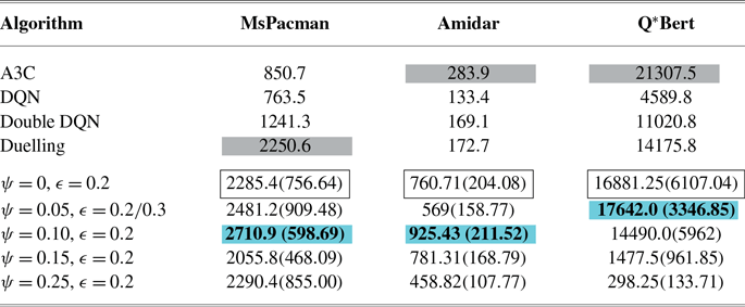
Results and Evaluation: To evaluate the agents, we investigate the averaged performance over 100 games after the training has been completed over 80M frames (Machado et al. Reference Machado, Bellemare, Talvitie, Veness, Hausknecht and Bowling2017). Table 2 depicts the averaged performance over five different runs, where each run contains the averaged score obtained over 100 testing games. It is observed that the Safe-A2OC with a controllability value of
 $\psi = 0.10$
in MsPacman not only outperforms the score achieved by the baseline A2OC (
 $\psi= 0$
) but also results in a smaller variance in the scores (values are shown in the braces). We observe a similar pattern in Q*Bert, wherein the Safe-A2OC (
 $\psi = 0.05$
) shows an improved robust performance over the A2OC (
 $\psi=0$
), achieving almost half of the variance of A2OC across multiple games.
In the game of Amidar, we note that Safe-A2OC outperforms the score achieved by A2OC, and the other state-of-the-art approaches (Nair et al. Reference Nair, Srinivasan, Blackwell, Alcicek, Fearon, Maria, Panneershelvam, Suleyman, Beattie, Petersen, Legg, Mnih, Kavukcuoglu and Silver2015; Wang et al. Reference Wang, de Freitas and Lanctot2015; Mnih et al. Reference Mnih, Badia, Mirza, Graves, Lillicrap, Harley, Silver and Kavukcuoglu2016; Van Hasselt et al. Reference Van Hasselt, Guez and Silver2016) using the primitive actions. Empirically, we observe that on adding an optimal amount of controllability value in options, an agent optimizing for low variance in the TD error learns better than the one optimizing only for the cumulative reward. Intuitively, minimizing the variance in the TD error as a measure of safety helps the agents avoid states with high intrinsic variability in the reward. Depending on the nature of the game itself, we observe different degrees of response to different levels of controllability in Q*bert, Amidar, and MsPacman. Based on the amount of variability in the reward structure, each game benefits differently in the performance. Overall, a consistent boost in the performance is demonstrated with the proposed approach once the training is completed.
ALE final scores: The performance is averaged over 100 games once the training is completed. The scores are averaged over five independent seeds. Scores in the boxes highlight the performance without controllability function (baseline), whereas aqua highlighted cells indicate the benefits of introducing our notion of safety in learning end-to-end options. Introducing controllability in options outperforms best performances of primitive actions (grey) in two out of three games analyzed here. Learning options with our notion of safety outperforms the baseline A2OC in all three games. A3C scores have been taken from Mnih et al. (Reference Mnih, Badia, Mirza, Graves, Lillicrap, Harley, Silver and Kavukcuoglu2016), DQN from Nair et al. (Reference Nair, Srinivasan, Blackwell, Alcicek, Fearon, Maria, Panneershelvam, Suleyman, Beattie, Petersen, Legg, Mnih, Kavukcuoglu and Silver2015), Double DQN from Van Hasselt et al. (Reference Van Hasselt, Guez and Silver2016), and Duelling from Wang et al. (Reference Wang, de Freitas and Lanctot2015).
 $\psi$
represents the degree of controllability. Values in the brackets indicate standard deviation across 100 games for 5 independent runs.

Learning curves in Atari games during training demonstrate that options with a controllability factor of
 $\psi=0.10$
learn better than the best-performing A2OC baseline (
 $\psi=0$
,
 $\epsilon=0.2$
). Higher value of
 $\psi$
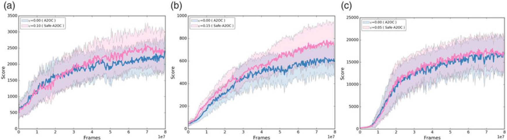
results in a poor performance. Performance is averaged across 5 independent seeds for each game.

Qualitative analysis in MsPacman: Our interpretation is that the Safe-A2OC agent understands the source of intrinsic variability in the reward due to explicitly optimizing for the variance in TD error. This results in Safe-A2OC agent to adopt the strategy of eating the large flashing power pellets, causing the ghosts to flee. The Safe-A2OC agent is able to survive longer and ends up accumulating more cumulative reward as opposed to the baseline A2OC agent. Here, we depict a sampled trajectory of the Safe-A2OC agent in comparison with the baseline A2OC agent.

We also inspect the learning curves during the training phase for all three Atari games. Figure 10 depicts the learning curves over 80M frames with varying controllability parameter. The results are averaged across five runs per game. In Amidar, we observe that with a specific degrees of controllability (
 $\psi = 0.15$
), options learned with our notion of safety (Safe-A2OC) outperform the baseline option-critic (A2OC). An improvement in the training performance also translates well to the testing phase as seen in Table 2. Interestingly, we observe that the performance of Safe-A2OC improves only marginally during the training phase in Ms-Pacman and is at-par with A2OC in Q*Bert. However, it is noteworthy that while we do not see much improvement in the training curves for both MsPacman and Q*Bert, during the testing phase, both these games show robust and improved performance. According to our interpretation, explicitly optimizing for the variance in TD error might not always result in a performance boost. Nevertheless, the proposed objective function makes the agent aware of intrinsic variability in the rewards. In the subsequent section, we will qualitatively analyze the behaviour of the trained agents.
Qualitative Observations: We are now interested in better understanding the behaviour of the trained agents. We observe that different values of
 $\psi$
control the degree to which an agent tends to be risk averse. A grid search over the different degrees of the controllability hyper parameter
 $\psi$
resulted in a narrow range of 0 to
 $0.15$
. For a very high value of
 $\psi>0.3$
, we observe that the agents become extremely risk-averse resulting in a poor performance. An optimum value of
 $\psi$
for all three games is obtained around
 $0.05-0.15$
. For a qualitative analysis, we also present the videos of the trained agents
Footnote 3
.
Upon visual inspection, we observe improvements in game playing strategies for Safe-OC agent as compared to its counterpart OC. The Safe-A2OC agents demonstrate relatively better understanding of the source of intrinsic variability in the reward structure. For instance, consider the game of MsPacman. The agent is tasked with eating all of the pellets in an enclosed maze while avoiding the four coloured ghosts. On consuming the power pellets in the environment, the ghosts turns blue and flee, resulting in bonus points. Frame-by-frame analysis shows that the Safe-A2OC agent is able to escape from the ghosts and stay alive longer when these ghosts are harmful in the context of a terminal state. Figure 11 depicts this observation, where the A2OC agent loses its first life relatively quickly as compared to the Safe-A2OC agent. These insights demonstrate that explicitly optimizing for the variance in TD error results in avoiding the visits to states with intrinsic variability in the rewards. Particularly, in MsPacman, the additional cost in the objective function helps the agent to understand the intrinsic variability in reward structure such as the behaviour observed upon the acquisition of the power pellets.
Furthermore, on close analysis of the behaviour of the Safe-OC agents, we observe that agents with extremely high value of
 $\psi$
are relatively more risk-averse but less exploratory in nature, thereby resulting in a poor performance (see Appendix 1). This corroborates with the findings in the learning curves as shown in Figure 10. For an optimal value of controllability regularizer (
 $\psi$
), we observe a balanced amount of risk aversion and, therefore, the agent adopts a behaviour which demonstrates a better understanding of intrinsic variability in the rewards structure. We perform a similar analysis for the game of Amidar and report similar insights in Appendix 2.
5 Discussion
In this work, we introduced Safe Option-Critic, a general framework that extends the idea of controllability from the primitive action space to the option-critic architecture. The key idea is to discourage the agent from visiting the state space with high uncertainty in their behavioural outcomes by constraining the variance in TD error. Recently, Sherstan et al. (Reference Sherstan, Ashley, Bennett, Young, White, White and Sutton2018) proposed a direct method to estimate the variance of
 $\lambda$
return. The authors proposed a Bellman operator for the variance that uses the square of the TD error. This work further supports our approach to estimating the risk using the squared TD error.
Our experiments in the tabular case empirically demonstrate the reduced variance in the return. Moreover, we observe a boost in the overall performance for both the tabular and the linear function approximation. Experiments in the ALE domain demonstrate that the agent can learn about the intrinsic variability in a large and complicated state-space using non-linear function approximation. Qualitative insights from ALE also demonstrate that the options with a notion of safety are more cautious in their behaviour and, therefore, result in improved overall performance.
Limitations and Future Work: In this work, we limit the return calculation until an option terminates. Using the n-step returns at the SMDP level is of potential interest for future work. Additionally, in this work, we assume that all the options are available in every state. In the context of safety, it would be of interest to understand the setting where options initiation sets are limited to a subset of the entire state space (Khetarpal et al. Reference Khetarpal, Klissarov, Chevalier-Boisvert, Bacon and Precup2020). One could also add a scheduler on the controllability regularizer
 $\psi$
over time. For instance,
 $\psi$
could be initiated with a small value to encourage exploration in the initial stages of learning, and gradually the value of
 $\psi$
could be increased to limit the exploration in the unsafe states.
Besides, a more formal analysis of the agent behaviour in ALE can provide a rigorous understanding of the interplay between learning the dynamics and the controllability parameter. For instance, studying the training and policy traces by human subjects is scope for future work.
In the proposed algorithm, we consider the notion of safety by accounting for the controllability of only the initial state-option pair. However, one can instead account for the variability due to the entire state-space by means of bootstrapping the target value function, aliasing due to the function approximation, and random resets to starting state. A potential direction for future work is to extend the controllability from the initial state-option pair to all the state-option pairs in the trajectory. This extension could potentially enhance the effects of the risk mitigation and speed up learning. The proposed notion of safety can also be extended to different levels of hierarchy, for example, a mixture of options with varying degrees of controllability can be learned.
Acknowledgements
The authors would like to thank Open Philanthropy for funding this work, Compute Canada for the computing resources, Herke van Hoof, Ayush Jain, Pierre-Luc Bacon, Gandharv Patil, Jean Harb, Martin Klissarov, Kushal Arora, for constructive discussions throughout the duration of this work, and the anonymous reviewers for the feedback on earlier drafts of this manuscript.
Competing interests
The authors declare none.
Appendix A
Appendix A.1 Experiments in the ALE domain
In this section, we show the results of training the agent in ALE games with multiple values of controllability parameter (
 $\psi$
). The results are averaged across five runs per game.
Appendix A.2 Qualitative observations in Amidar
We also analyze the behaviour of the trained agents in the game of Amidar as shown in Figure A2. Just as MsPacman, in Amidar, the agent is faced with enemies, who upon contact can kill the agent. The agent’s goal is to paint the rectangular boards by traversing all the sides of the board. Upon painting all the four corners of a rectangle, the agent is briefly equipped with the ability to make the enemies ineffective for a short duration, analogous to consuming the power-pellets in MsPacman.
Figure A2 depicts the final frame in three games played by the trained agents. Safe-A2OC agents end up painting more rectangles than the A2OC agent. There is inherent variability in the reward structure of this environment. Since painting all four sides of the rectangle results in the ability to make the enemies ineffective, Safe-A2OC agents are able to understand this structure relatively better by directly optimizing for the variance in TD error. Therefore, Safe-A2OC agents result in painting more rectangles in the board as depicted, leading to a higher cumulative reward than the baseline agent.
Learning curves during training for ALE games: Higher degrees of controllability (
 $\psi>0.15$
) result in reduced exploration and adversely affect the performance. We observe that the agents trained with an extremely high value of
 $\psi$
are relatively more risk averse as compared to smaller values of controllability.

Qualitative analysis in Amidar: We here demonstrate the final frames from randomly sampled 3 games played by the trained agents. Safe-A2OC agent learns to paint relatively more rectangles as compared to the A2OC agent as painting all sides of a rectangle results in making the ghosts ineffective, and thus increases the cumulative return. Amidar offers intrinsic variability in the reward structure, and our approach empowers the agents to understand it better.