1 Introduction
Most flows over bluff bodies are featured by unsteady quasi-periodic vortex shedding, forming the well-known Kármán vortex street (Williamson Reference Williamson1996). The periodic vortex field is reflected in the pressure distribution and fluctuating drag and lift forces acting on the body, which can lead to serious structural damage due to vortex-induced vibrations (Bearman Reference Bearman1984; Sarpkaya Reference Sarpkaya2004). A variety of active and passive methods have been proposed to control the flow and combat the undesired flow–structure interactions (Choi, Jeon & Kim Reference Choi, Jeon and Kim2008). The common aim is to manipulate the frequency of oscillations and to reduce the amplitude of the drag and lift forces, both of which are of utmost importance in a wide range of practical applications.
A vast amount of the research on flow over a cylinder representing a model bluff body configuration reports on the effect of various control methods leading to specific changes of the flow features. Among these are the application of steady and periodic blowing/suction of the fluid through the cylinder wall (Lin, Towfighi & Rockwell Reference Lin, Towfighi and Rockwell1995; Arcas & Redekopp Reference Arcas and Redekopp2004; Chen et al. Reference Chen, Xin, Xu, Li, Ou and Hu2013), distributed forcing (Kim & Choi Reference Kim and Choi2005; Poncet et al. Reference Poncet, Hildebrand, Cottet and Koumoutsakos2008), various geometric modifications including roughness (Shih et al. Reference Shih, Wang, Coles and Roshko1993), dimples (Bearman & Harvey Reference Bearman and Harvey1993), splitter plates (Roshko Reference Roshko1954), grooves (Lim & Lee Reference Lim and Lee2002), small secondary cylinders (Strykowski & Sreenivasan Reference Strykowski and Sreenivasan1990) and similar means (Lam & Lin Reference Lam and Lin2009; Gao et al. Reference Gao, Chen, Li and Hu2017), electromagnetic forcing (Kim & Lee Reference Kim and Lee2000), hydrophobic surfaces (You & Moin Reference You and Moin2007), steady and oscillating rotation (Okajima, Takata & Asanuma Reference Okajima, Takata and Asanuma1975; Mittal & Kumar Reference Mittal and Kumar2003), in-line and transverse oscillations (Bearman Reference Bearman1984), etc. While the approaches mentioned above represent passive and active open-loop control methods (without the feedback), there is a branch of control theory dealing with active closed-loop methods (Moin & Bewley Reference Moin and Bewley1994; Brunton & Noack Reference Brunton and Noack2015) where the controlling devices are activated according to the information on flow characteristics received from sensors.
A recent example of the application of adjoint-based optimal control of a low-amplitude rotary-oscillating cylinder at low Reynolds numbers (
 $75<Re<200$
) by Flinois & Colonius (Reference Flinois and Colonius2015) suggested a delicate connection between the phase of the cylinder rotation and wake oscillations required for a successful drag reduction, as also discussed by Protas & Styczek (Reference Protas and Styczek2002) and Bergmann, Cordier & Brancher (Reference Bergmann, Cordier and Brancher2005). The self-tuning forcing provided by a ‘smart’ optimization procedure seems very promising for control purposes. However, earlier experiments with feedback control based on instantaneous velocity point measurements in the wake at
 $Re=6.7\times 10^{3}$
and
 $2.0\times 10^{4}$
provided only a minor drag reduction effect (Fujisawa, Kawaji & Ikemoto Reference Fujisawa, Kawaji and Ikemoto2001). Thus, it is not very clear if the practical implementation can be robust and straightforward at high Reynolds numbers for a fully turbulent motion.
We investigate the efficiency of cylinder rotary oscillations in manipulating lift, drag and velocity fluctuations in the wake by performing a parametric study in a wide range of
 $\unicode[STIX]{x1D6FA}$
and
 $f$
values defined below at high subcritical Reynolds number
 $Re=1.4\times 10^{5}$
which is at least an order of magnitude higher than previously explored in the literature. A simple case of sinusoidal in time rotary oscillations of the cylinder represents a two-dimensional forcing active open-loop control method where the forcing targets the boundary layer and not directly the wake region (Choi et al.
Reference Choi, Jeon and Kim2008). The tangential velocity of the cylinder wall is forced to oscillate in time according to the following relation:
 $$\begin{eqnarray}U_{\unicode[STIX]{x1D703}}^{wall}=\unicode[STIX]{x1D714}_{e}R\sin (2\unicode[STIX]{x03C0}f_{e}t),\end{eqnarray}$$
where
 $\unicode[STIX]{x1D714}_{e}$
is the angular velocity representing the amplitude of oscillation,
 $R$
the radius of the cylinder and
 $f_{e}$
the imposed frequency. After normalization with the uniform inflow velocity
 $U_{\infty }$
and diameter of the cylinder
 $D$
, the wall velocity is:
 $$\begin{eqnarray}U_{\unicode[STIX]{x1D703}}^{wall}/U_{\infty }=\unicode[STIX]{x1D6FA}^{\ast }\sin (2\unicode[STIX]{x03C0}f_{e}^{\ast }t^{\ast })=\unicode[STIX]{x1D6FA}^{\ast }\sin \unicode[STIX]{x1D711}^{\ast },\end{eqnarray}$$
where
 $\unicode[STIX]{x1D6FA}^{\ast }=\unicode[STIX]{x1D714}_{e}D/2U_{\infty }=\unicode[STIX]{x1D6FA}_{e}/U_{\infty }$
with
 $\unicode[STIX]{x1D6FA}_{e}=\unicode[STIX]{x1D714}_{e}D/2$
,
 $t^{\ast }=tU_{\infty }/D$
and
 $f_{e}^{\ast }=f_{e}D/U_{\infty }$
is the Strouhal number of the imposed oscillations and
 $\unicode[STIX]{x1D711}^{\ast }=2\unicode[STIX]{x03C0}f_{e}^{\ast }t^{\ast }$
is the rotational phase. Further below we drop the superscript
 $^{\ast }$
assuming that all variables are given in non-dimensional forms (scaled by
 $U_{\infty }$
and
 $D$
). Thus, the problem is governed by three parameters, i.e. the Reynolds number
 $Re=U_{\infty }D/\unicode[STIX]{x1D708}$
where
 $\unicode[STIX]{x1D708}$
is the kinematic viscosity of the fluid, the non-dimensional amplitude and frequency of oscillations,
 $\unicode[STIX]{x1D6FA}$
and
 $f=f_{e}/f_{0}$
, respectively, where
 $f_{0}$
is the natural vortex-shedding frequency without forcing. The parameters of interest are the drag and lift coefficients defined as
 $$\begin{eqnarray}C_{D}=\frac{F_{D}}{\frac{1}{2}\unicode[STIX]{x1D70C}U_{\infty }^{2}D},\quad C_{L}=\frac{F_{L}}{\frac{1}{2}\unicode[STIX]{x1D70C}U_{\infty }^{2}D},\end{eqnarray}$$
where
 $F_{D}$
and
 $F_{L}$
are the forces acting on the cylinder (per unit length) along the flow direction (drag) and perpendicular to it (lift),
 $\unicode[STIX]{x1D70C}$
is the fluid density.
Previous simulations for relatively low Reynolds numbers were usually performed using a grid-free Lagrangian approach called the vortex method (VM) or standard two-dimensional (2-D) or three-dimensional (3-D) direct numerical simulations (DNS) of the Navier–Stokes equations, while for higher
 $Re$
numbers large-eddy simulation (LES) was the usual compromise between accuracy and computing time. As shown by Poncet (Reference Poncet2002, Reference Poncet2004) rotary oscillations effectively suppress three-dimensional instabilities justifying the use of 2-D simulations at low
 $Re$
. He et al. (Reference He, Glowinski, Metcalfe, Nordlander and Periaux2000) performed 2-D DNS at
 $Re=200$
and
 $10^{3}$
and searched for optimal control parameters calculating the gradient of the cost function. These authors observed a decrease of the time-averaged
 $C_{D}$
of around 30 % and 60 % for two
 $Re$
numbers, respectively, with
 $f=3.8$
,
 $\unicode[STIX]{x1D6FA}=6$
and
 $f=2.61$
,
 $\unicode[STIX]{x1D6FA}=5.5$
. A similar study has been performed by Homescu, Navon & Li (Reference Homescu, Navon and Li2002). Cheng, Chew & Luo (Reference Cheng, Chew and Luo2001) used VM simulations to support the results of He et al. (Reference He, Glowinski, Metcalfe, Nordlander and Periaux2000) showing a 40 % decrease of
 $C_{D}$
at
 $f=4$
,
 $\unicode[STIX]{x1D6FA}=3$
and
 $Re=10^{3}$
and even 60 % at
 $f=2.61$
,
 $\unicode[STIX]{x1D6FA}=2.75$
and the same
 $Re$
number. The method has not proven to be very energetically efficient at low
 $Re$
number (Protas & Wesfreid Reference Protas and Wesfreid2002; Bergmann, Cordier & Brancher Reference Bergmann, Cordier and Brancher2006), suggesting that the study be extended towards higher
 $Re$
.
For
 $Re=1.5\times 10^{4}$
, the experiments by Tokumaru & Dimotakis (Reference Tokumaru and Dimotakis1991) showed a dramatic decrease of
 $C_{D}$
by around 85 % with the optimal values of
 $\unicode[STIX]{x1D6FA}$
and
 $f$
being around
 $2$
and
 $4$
, respectively, attracting more attention to this control method. Shiels & Leonard (Reference Shiels and Leonard2001) performed 2-D simulations in the range
 $150<Re<1.5\times 10^{4}$
using VM and qualitatively confirmed the results of Tokumaru & Dimotakis (Reference Tokumaru and Dimotakis1991). However, the maximum reduction achieved was around 70 % at
 $f=5.3$
, (The value is normalized using the natural vortex-shedding frequency taken from Du & Dalton (Reference Du and Dalton2013).)
 $\unicode[STIX]{x1D6FA}=2$
and
 $Re=1.5\times 10^{4}$
. They showed that the mechanism of drag reduction caused by a train of detaching vortices in the boundary layer is only effective at
 $Re>3.0\times 10^{3}$
due to viscous dumping of separation at lower
 $Re$
numbers. Sengupta, Deb & Talla (Reference Sengupta, Deb and Talla2007) used a genetic algorithm and 2-D DNS to determine
 $\unicode[STIX]{x1D6FA}$
and
 $f$
which minimize the drag coefficient at
 $Re=1.5\times 10^{4}$
. They found the optimal value to be around
 $\unicode[STIX]{x1D6FA}=3.0$
and
 $f=3.6$
leading to
 $C_{D}=0.42$
compared to
 $C_{D}=1.62$
in the non-rotating case. Du & Dalton (Reference Du and Dalton2013) performed 2-D DNS and 3-D LES at
 $Re=150$
and
 $1.5\times 10^{4}$
, respectively, sufficiently reducing the drag coefficient down to
 $C_{D}=0.46$
for
 $\unicode[STIX]{x1D6FA}=2.0$
and
 $f=2.5$
in the latter case. They also pointed at uncertainties of the indirect method for drag estimation employed by Tokumaru & Dimotakis (Reference Tokumaru and Dimotakis1991) which could lead to underestimation of
 $C_{D}$
. Shiels & Leonard (Reference Shiels and Leonard2001) analysed the efficiency of the rotary-oscillation control in terms of the power saving criterion, defined as the ratio of the power gain by drag reduction versus the power spent to oscillate the cylinder.
In the following, § 2 provides information on the flow configuration, computational details and on the verification and validation of the applied Reynolds-stress model (RSM). In § 3 we present and discuss the computational results for a variety of cases considered. Section 4 discusses the mechanism of the drag reduction due to rotary oscillations of the cylinder wall, whereas in § 5 we analyse the potential, efficiency and benefits of the considered control method in terms of the ratio of the power saved and power expended.
2 Computational details and model validation
The computations were performed using the in-house unstructured finite-volume code T-FlowS developed at TU Delft (Ničeno & Hanjalić Reference Ničeno and Hanjalić2005) and used over the years for LES, Reynolds-averaged Navier–Stokes (RANS) and hybrid solutions in the research of a variety of turbulent flows and transport processes. The three-dimensional unsteady RANS (URANS) solutions were obtained on a mesh containing
 $2.24\times 10^{6}$
cells using the wall-integrated Reynolds-stress model (RSM) of Jakirlić & Hanjalić (Reference Jakirlić and Hanjalić2002), whereas the dynamic Smagorinsky subgrid-scale model was employed in the reference LES on a mesh of
 $13.4\times 10^{6}$
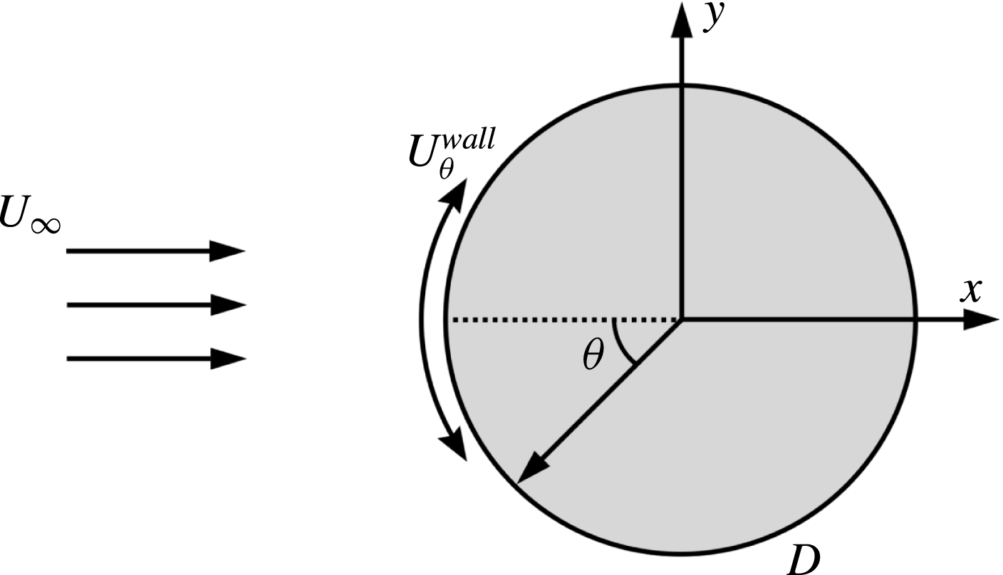
cells. The computational domain, shown in figure 1, was
 $L_{x}\times L_{y}=25\times 20$
in the streamwise and cross-wise directions while the spanwise length was
 $L_{z}=2$
for URANS and
 $3$
for LES. (Although the present spanwise length
 $L_{z}$
does not fully resolve the oblique waves (Williamson Reference Williamson1989), recent studies at
 $Re=1.3\times 10^{5}$
(Cao & Tamura Reference Cao and Tamura2015) suggest that the chosen length gives sufficiently accurate drag coefficients. Also, the two-dimensionalization due to rotary oscillations suppressing this kind of instability is described below.) The centre of the cylinder was placed at
 $10D$
from the inflow boundary. Slip conditions were set at the top and bottom boundaries, the convective outflow condition was imposed at the outlet and the time-dependent tangential velocity on the cylinder wall was calculated every time step according to (1.2). Periodic conditions were imposed on the side boundaries along the spanwise direction. The inflow was defined by the uniform velocity
 $U_{\infty }$
and zero free-stream turbulence. The time steps in all computations were chosen so that Courant–Friedrichs–Lewy (CFL) number was around 1. The LES simulations were conducted with a time step
 $\unicode[STIX]{x0394}t=5\times 10^{-4}$
while for the RSM
 $\unicode[STIX]{x0394}t=10^{-3}$
. For URANS the first grid point satisfied the condition
 $\unicode[STIX]{x0394}r^{+}<3$
and
 $\unicode[STIX]{x0394}r^{+}<1.0{-}1.8$
corresponding to the areas before and after separation, respectively, slightly varying for different
 $\unicode[STIX]{x1D6FA}$
and
 $f$
. Here the non-dimensionalization was performed in wall units with the ‘
 $+$
’ superscript using the friction velocity and viscosity. The cell size along the cylinder wall satisfied
 $(R\unicode[STIX]{x0394}\unicode[STIX]{x1D703})^{+}<70/40$
. For LES these numbers were much lower with
 $\unicode[STIX]{x0394}r^{+}<1.4/0.8$
,
 $(R\unicode[STIX]{x0394}\unicode[STIX]{x1D703})^{+}<90/35$
and
 $\unicode[STIX]{x0394}z^{+}<200/100$
calculated before/after the separation point.
Schematic picture of flow around a rotating cylinder.

In the previous work (Palkin et al.
Reference Palkin, Mullyadzhanov, Hadžiabdić and Hanjalić2016) we assessed the performance of the second-moment closure model (RSM) described here in parallel with an elliptic-relaxation linear eddy-viscosity model (EVM), as representative of advanced EVMs, in a cross-flow over an infinite cylinder with reference to our LES, available DNS and experiments at two Reynolds numbers,
 $Re=3.9\times 10^{3}$
and
 $1.4\times 10^{5}$
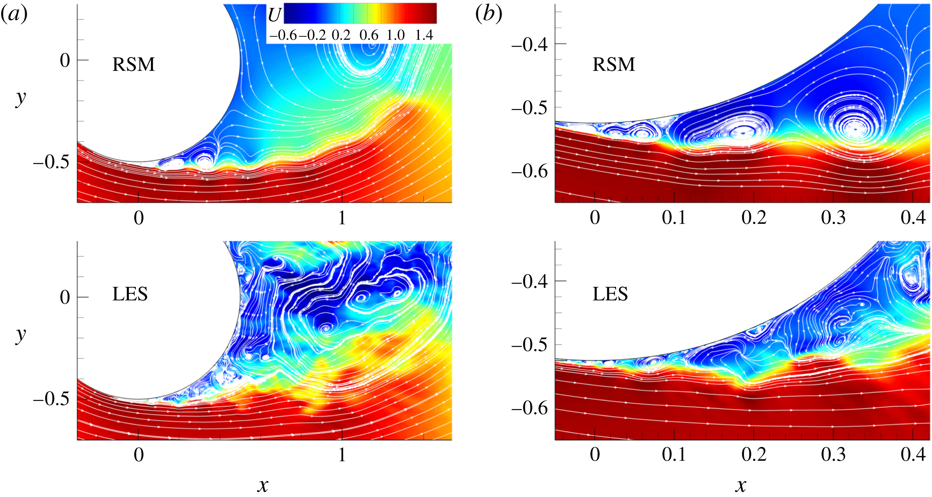
. The URANS results show that, despite the conceptual limitations, both models (EVM and RSM) reproduced the major flow features, but the RSM proved to be far superior, replicating closely the LES-revealed subtle details of the laminar separation dynamics, subsequent transition to turbulence, multiple-vortex systems, their evolution including the low-frequency modulation, and dynamic characteristics – vorticity intensity, frequency and amplitudes, as well as their origin, pattern, size and strength, as illustrated in figure 2. The key of the success of the RSM in the case considered is the better reproduction of the natural stress anisotropy and of the misalignment of the eigenvectors of the strain-rate tensor and the traceless Reynolds-stress tensor – both inaccessible to eddy-viscosity models. This leads to a much lower effective eddy viscosity in the RSM and consequently to its higher sensitivity and receptivity to inherent instabilities compared to the EVMs. These findings are believed to extend to other bluff bodies and other high-
 $Re$
flows dominated by strong semi-deterministic vortex structures.
Instantaneous streamwise velocity field from LES and RSM at the same phase of the lift coefficient showing the multi-point wall-flow separation/reattachment and multiple vortices in the wall region. (b) Shows a blow up of the separation region given in (a). Adapted from Palkin et al. (Reference Palkin, Mullyadzhanov, Hadžiabdić and Hanjalić2016).

Table 1 shows a comparison of the main statistical properties of the flow obtained from LES and URANS demonstrating the accuracy of the URANS approach for this flow. Especially important for the present study is that the RSM reproduced a drag coefficient
 $C_{D}=1.24$
that agrees very well with the experimental value
 $C_{D}=1.23$
reported by Cantwell & Coles (Reference Cantwell and Coles1983). We further performed several additional LES simulations for the cylinder with rotary oscillations in order to assess the URANS approach for this particular set-up. We simulated the set-up which produces high drag reduction
 $f=2.5$
and
 $\unicode[STIX]{x1D6FA}=2$
on the same mesh used for LES of flow over a stagnant cylinder as well as even a higher-frequency forcing with
 $f=4$
and
 $\unicode[STIX]{x1D6FA}=2$
. Some results for
 $f=2.5$
and
 $\unicode[STIX]{x1D6FA}=2$
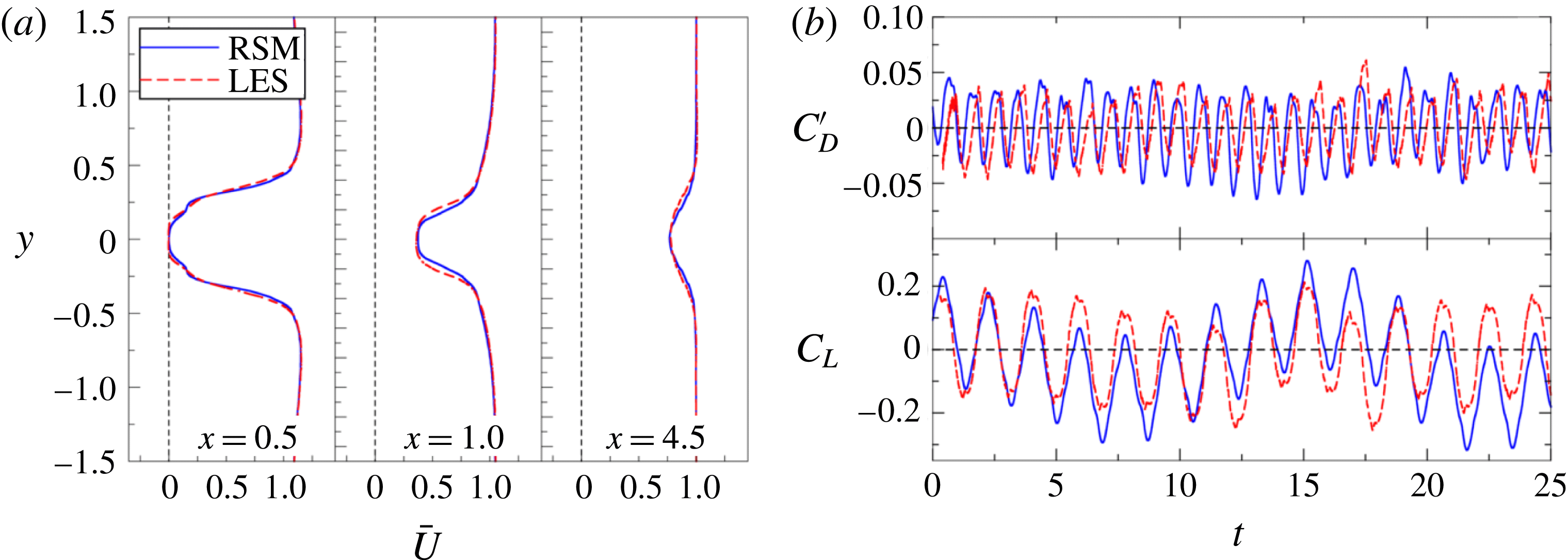
are compared in figure 3 where the oscillating cylinder URANS shows a similar level of accuracy as reported by Palkin et al. (Reference Palkin, Mullyadzhanov, Hadžiabdić and Hanjalić2016) for the unforced cylinder flow. The URANS reproduces successfully the mean velocity, figure 3(a), but also the dynamic flow features illustrated by the oscillations of the drag and lift coefficients, shown in figure 3(b). A close agreement for the drag coefficient is obtained with
 $C_{D}=0.25$
provided by LES and
 $C_{D}=0.28$
by URANS. For the case with
 $f=4$
and
 $\unicode[STIX]{x1D6FA}=2$
the drag coefficient is also well reproduced with
 $C_{D}=0.18$
(LES) and
 $C_{D}=0.16$
(URANS). This validation confirms that the RSM approach is a reliable tool to simulate a rotary-oscillating cylinder in cross-flow, justifying its use in the further parametric studies of a number of cases with different imposed frequencies and amplitudes of the forced rotary oscillations.
Comparison of RSM (solid line) and LES (dashed) results for
 $f=2.5$
and
 $\unicode[STIX]{x1D6FA}=2$
. (a) Mean streamwise velocity profiles at
 $x/D=0.5$
,
 $1.0$
,
 $4.5$
. (b) The time evolution of the drag coefficient fluctuations
 $C_{D}^{\prime }$
and lift coefficient
 $C_{L}$
.

Comparison of the mean drag coefficient (
 $C_{D}$
), pressure base coefficient (
 $C_{pb}$
), separation angle (
 $\unicode[STIX]{x1D703}_{s}$
), recirculation zone length (
 $L_{r}$
) and vortex-shedding frequency (
 $f_{0}$
) obtained from LES and RSM at
 $Re=1.4\times 10^{5}$
without rotation.

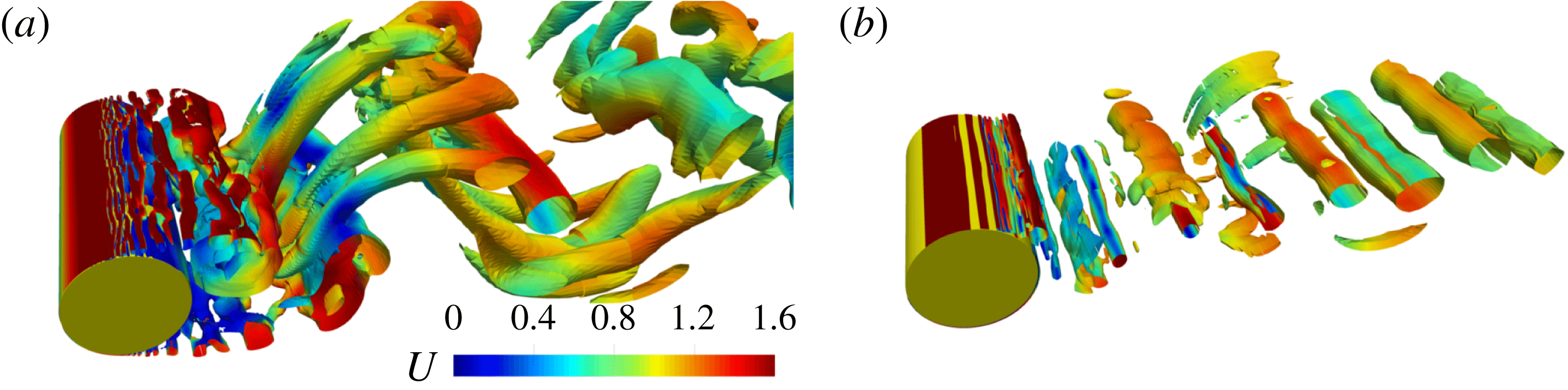
Isosurface of
 $Q=0.5$
for (a) non-rotating case and (b)
 $f=2.5$
,
 $\unicode[STIX]{x1D6FA}=2$
coloured with instantaneous streamwise velocity from RSM.

3 Results and discussion
To visualize the flow changes imposed by rotation, figure 4 shows the isosurface of the
 $Q$
-criterion computed from RSM for non-rotating case and
 $f=2.5$
,
 $\unicode[STIX]{x1D6FA}=2$
where
 $Q=(\unicode[STIX]{x1D6FA}_{ij}\unicode[STIX]{x1D6FA}_{ij}-\unicode[STIX]{x1D61A}_{ij}\unicode[STIX]{x1D61A}_{ij})/2$
, with
 $\unicode[STIX]{x1D6FA}_{ij}$
and
 $\unicode[STIX]{x1D61A}_{ij}$
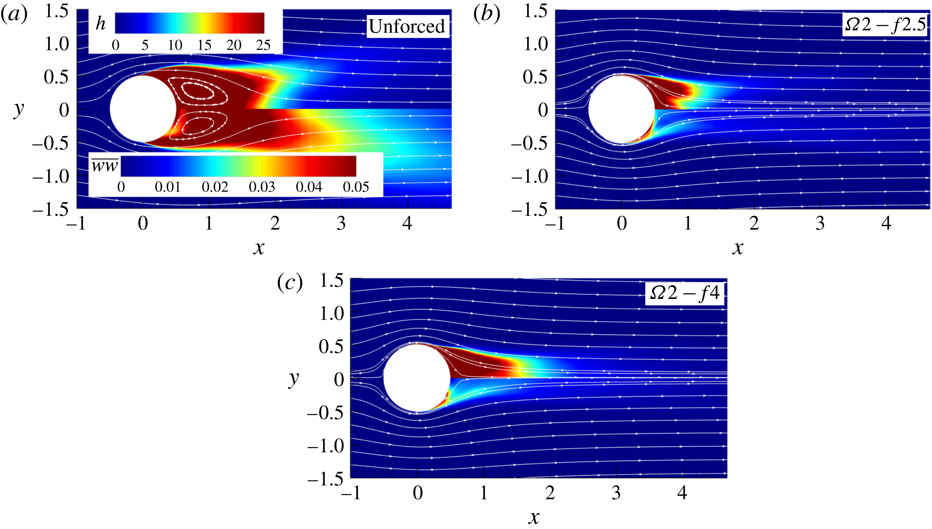
being the symmetric and antisymmetric components of the velocity gradient tensor. While the flow over a stagnant cylinder produces three-dimensional coherent structures and a relatively wide wake, the rotation suppresses three-dimensional evolution of large-scale structures and enforces the Kármán vortex street, keeping the rolls almost two-dimensional. Figure 5 shows the sum of time-averaged squared
 $x$
and
 $y$
vorticity components and spanwise fluctuations supporting the tendency towards two-dimensionalization with the addition of rotary oscillations compared to the unforced case. Further, we discuss the results for some of the considered cases with eight different rotation frequencies,
 $f=f_{e}/f_{0}=0.5$
,
 $1$
,
 $1.5$
,
 $2$
,
 $2.5$
,
 $3$
,
 $4$
and
 $5$
, and three rotational amplitudes,
 $\unicode[STIX]{x1D6FA}=1$
,
 $2$
and
 $3$
. The computations are denoted as
 $\unicode[STIX]{x1D6FA}X-fY$
, where
 $X$
is the non-dimensional value of the forcing amplitude and
 $Y$
the forcing frequency.
Comparison of time-averaged squared vorticity based on two components
 $h=(\overline{\unicode[STIX]{x1D714}_{x}^{2}}+\overline{\unicode[STIX]{x1D714}_{y}^{2}})/2$
(upper halves) and spanwise velocity fluctuations
 $\overline{ww}$
(lower halves) from LES for the unforced case,
 $\unicode[STIX]{x1D6FA}2-f2.5$
and
 $\unicode[STIX]{x1D6FA}2-f4$
.

3.1 Unforced cylinder
The URANS and LES of flow over a stationary cylinder at the same
 $Re$
number have been presented and discussed in detail in Palkin et al. (Reference Palkin, Mullyadzhanov, Hadžiabdić and Hanjalić2016). However, before analysing the effects of the cylinder rotation on flow modifications and drag reduction, we recall briefly some salient features of the flow dynamics around a stagnant cylinder. This dynamics is governed by the periodic vortex shedding at the top and bottom of the cylinder. At the subcritical
 $Re$
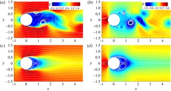
number considered, the flow separation is laminar and transition occurs in the shear layer downstream, reinforced by the fluid recirculation. The vortices formed in the shear layer coalesce with neighbouring ones, forming large vortex structures that interact with their twins from the other side of the cylinder. The process is quasi-periodic as the incoming flow periodically supplies more streamwise momentum to the top or bottom side of the cylinder, as shown in figure 6(a,b). The side of the cylinder with excessive momentum is characterized by eddies with higher vorticity due to the more intensive shear. The large vortex, generated by the coalescence of small vortices, acts as an obstacle for the incoming fluid and, as a result, more momentum is supplied to another side of the cylinder. The natural shedding frequency
 $f_{0}$
is the frequency of appearance of the large vortical structures that switch the momentum imbalance from one to another side of the cylinder. For high Reynolds numbers the drag coefficient is almost entirely due to the difference in the pressure in the front and back sides of the cylinder. The low-pressure zone is determined by the presence of strong vortical structures in the wall vicinity, as seen in figure 6(b). Figure 6(c,d) show the fields of the mean streamwise velocity and pressure. The mean recirculation bubble is symmetric with a length of
 $0.67D$
for the present flow parameters. The mean pressure field shows a low-pressure zone starting at the mean position of the initial separation point and extending to the rear of the cylinder. However, the minimum mean pressure zone appears away from the wall further downstream at the location where the large-scale structures reach the maximum size.
(a,b) Instantaneous and (c,d) mean fields of streamwise velocity and pressure for the unforced case.

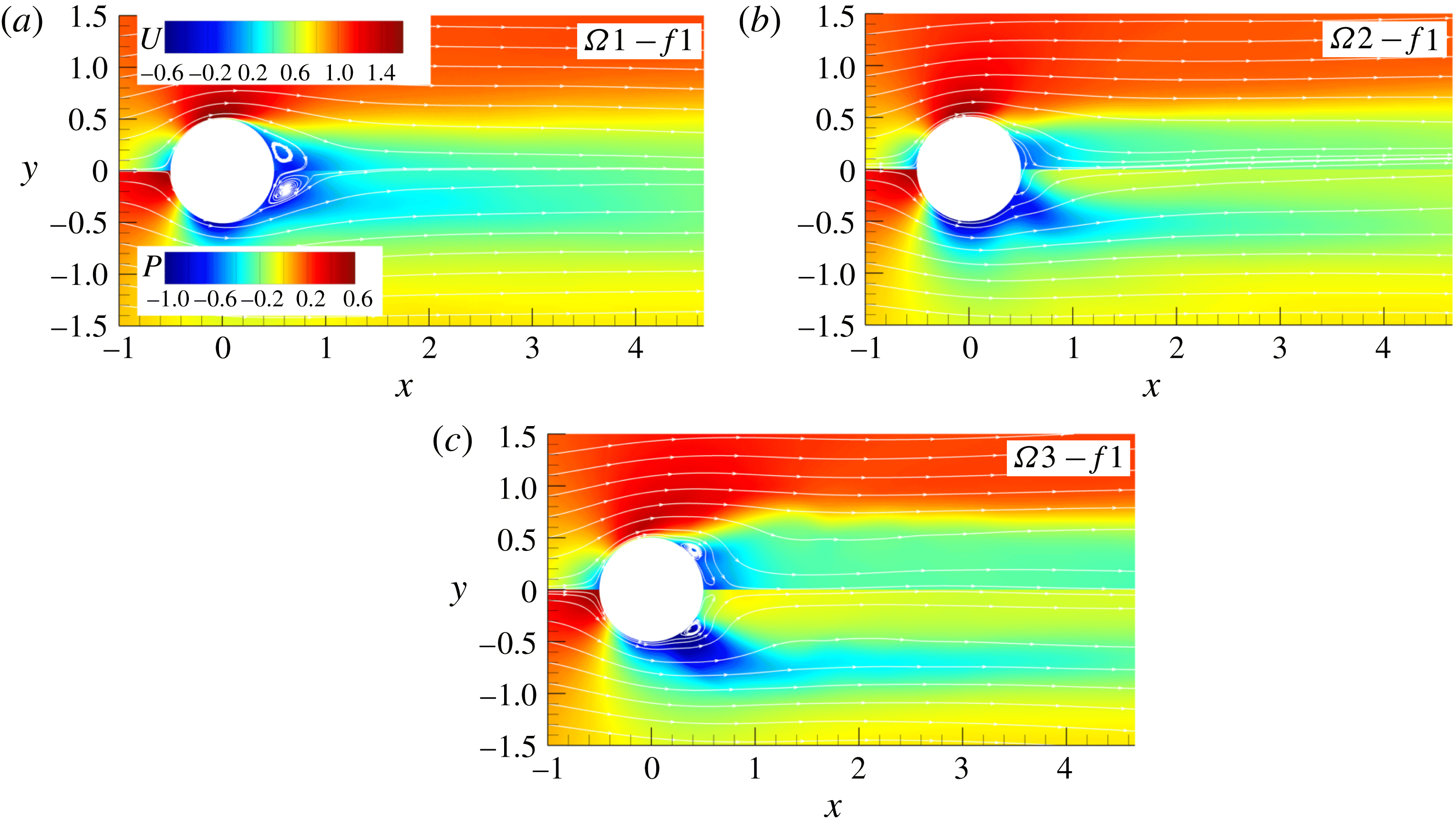
Mean streamwise velocity and pressure fields for
 $f=1$
and different amplitudes.

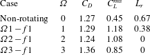
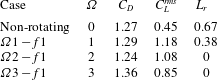
Mean drag coefficient (
 $C_{D}$
), root mean square of the lift coefficient (
 $C_{L}^{rms}$
) and the recirculation zone length (
 $L_{r}$
) for different rotational amplitudes and forcing frequency
 $f=1$
.
3.2 Rotary oscillations: forcing frequency
 $f=1$

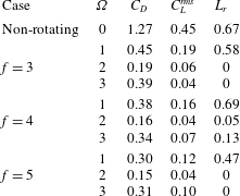
The selected integral characteristics of the flow with forcing frequency equal to that of the natural vortex shedding for three forcing amplitudes are listed in table 2. The mean drag coefficient is not much different (within 5 %) for all three cases compared to the unforced case. It slightly increases for amplitudes
 $\unicode[STIX]{x1D6FA}=1$
and 3, and decreases for
 $\unicode[STIX]{x1D6FA}=2$
compared to the reference non-rotational value. Du & Dalton (Reference Du and Dalton2013) reported an increase of 18 % in
 $C_{D}$
for the same forcing frequency and
 $\unicode[STIX]{x1D6FA}=2$
, but for an order of magnitude smaller Reynolds number. Interestingly, the small differences in the mean drag coefficient do not reflect the observed significant change of the flow pattern and its dynamics compared to the non-rotating case. Note that fluctuations of
 $C_{L}$
significantly increase for oscillating cases, table 2. Figure 7 shows mean fields of streamwise velocity and pressure for three forcing amplitudes. The recirculation zone is reduced by approximately 40 % for the lowest amplitude
 $\unicode[STIX]{x1D6FA}=1$
, while the recirculation bubble disappears completely for
 $\unicode[STIX]{x1D6FA}=2$
and 3. The mean pressure fields, shown in the lower halves of figure 7, reflect the changes in the velocity fields due to the oscillations. For all three forcing amplitudes the low pressure zone is attached to the cylinder, but spreads more and more laterally as the amplitude increases. The pressure distribution is markedly different from that in the non-rotating case where the low pressure zone is located on the centreline behind the cylinder further downstream, figure 6(d). In the rear of the cylinder the mean pressure is still negative for
 $\unicode[STIX]{x1D6FA}=1$
, but it becomes close to zero for
 $\unicode[STIX]{x1D6FA}=2$
and positive for
 $\unicode[STIX]{x1D6FA}=3$
. Surprisingly, the lateral shift of the negative pressure zones apparently does not affect the mean drag coefficient as shown in table 2.
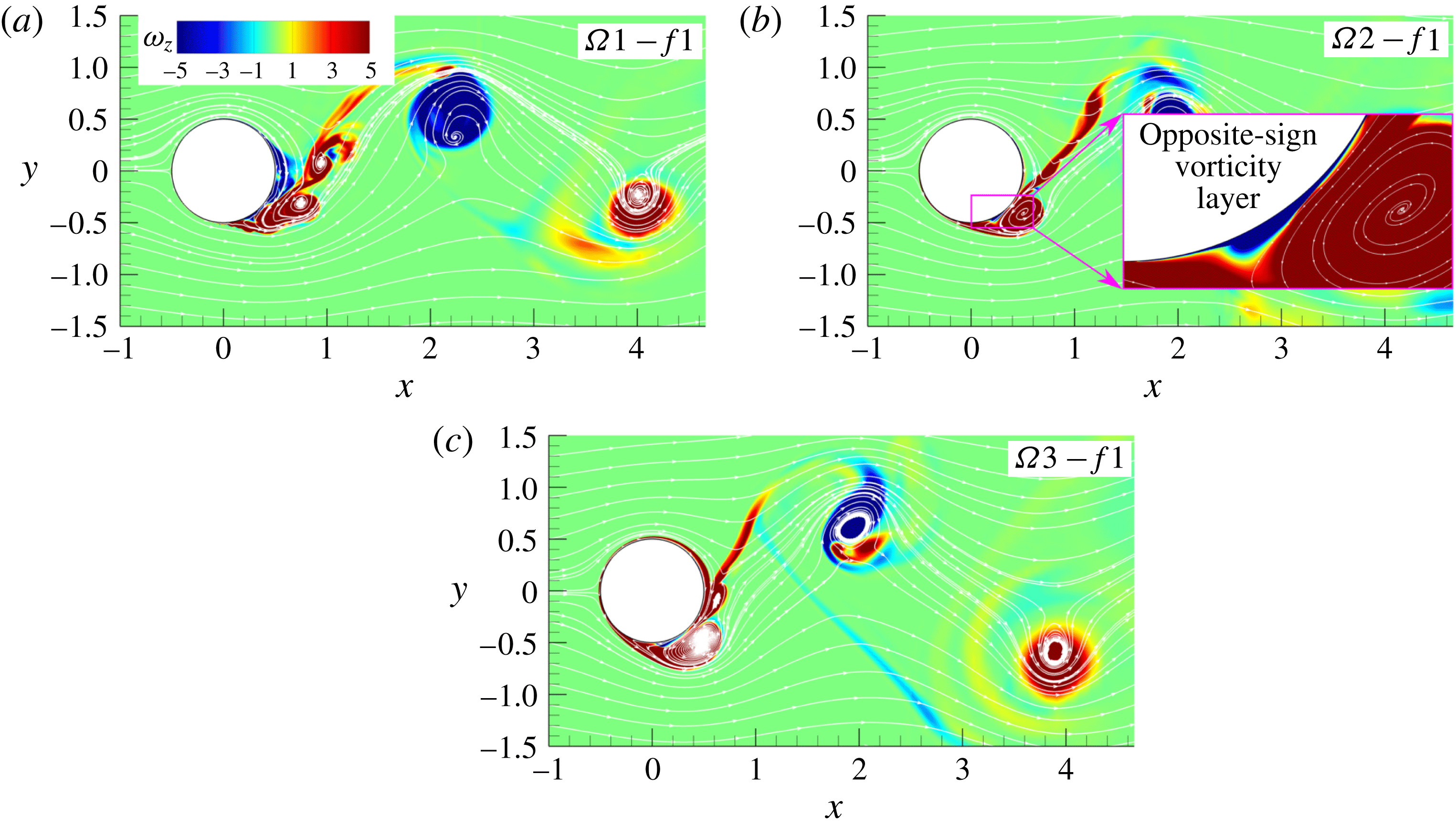
The instantaneous spanwise vorticity field, figure 8, shows that for all three tested amplitudes the cylinder releases one vortex per cycle. For all three amplitudes the wake structure is synchronized with the cylinder oscillation which persists downstream beyond the domain length of 15
 $D$
. However, only for
 $\unicode[STIX]{x1D6FA}=3$
does the boundary layer near the cylinder laminarize due to strong rotary oscillations suppressing the smaller-scale vortical dynamics which allows to detect a lock-on regime, as described below. This type of wake organization corresponds to mode II of Tokumaru & Dimotakis (Reference Tokumaru and Dimotakis1991). The flow shares some common characteristics for all three tested amplitudes. As reported by Cheng et al. (Reference Cheng, Chew and Luo2001), Du & Dalton (Reference Du and Dalton2013) among others, an oscillation frequency of the cylinder that is close or equal to
 $f_{0}$
produces much stronger vortices due to the additional vorticity generated by rotation. This resonance leads to higher values of the root mean square of
 $C_{L}$
compared to the non-rotating case, see table 2. A large vortex structure is shed every cycle and does not strongly interact with neighbouring vortices in the wake with opposite vorticity. The wake width becomes larger due to stronger vortex structures in the shear layer. Once the cylinder changes its rotational direction, a thin vorticity layer starts to grow between the wall and rotationally generated separation bubble that was attached to the wall until that moment, see the inset in figure 8(b). As the bubble and the newly formed layer have opposite vorticity signs, the separation bubble detaches from the wall and evolves into the main vortex, figure 8.
Instantaneous fields of spanwise vorticity for three amplitudes and
 $f=1$
.

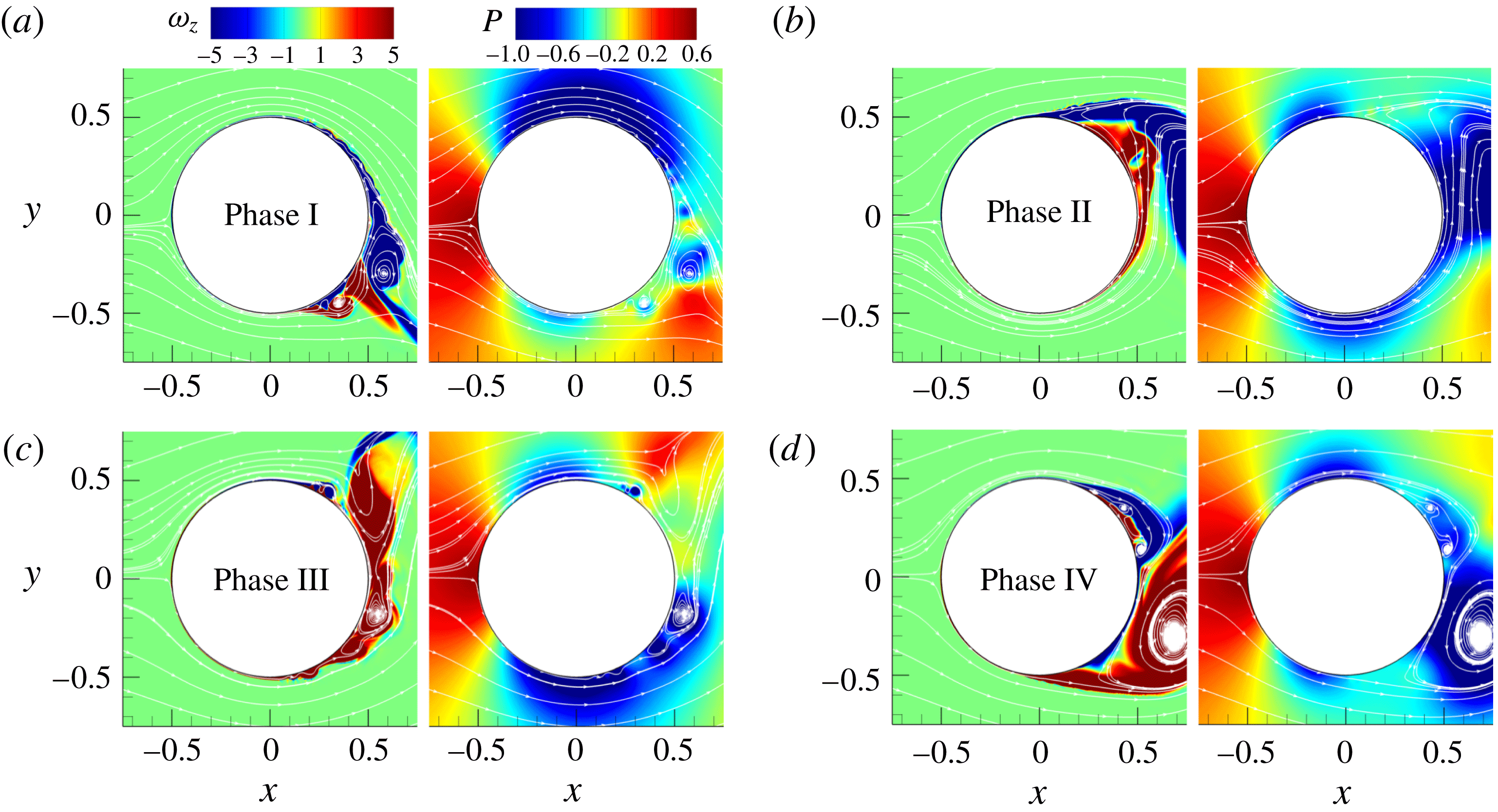
Instantaneous fields of spanwise vorticity and pressure for
 $\unicode[STIX]{x1D6FA}1-f1$
.

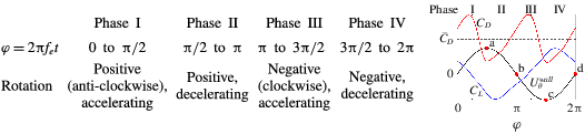
Specification of the characteristic cycle phases. Plot on the right shows the typical time history of
 $C_{D}$
(red line),
 $C_{L}$
(blue) and
 $U_{\unicode[STIX]{x1D703}}^{wall}$
(black) against the rotation phase
 $\unicode[STIX]{x1D711}$
.
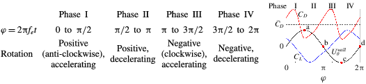
In order to understand the impact of rotation on the drag and lift coefficient, we look into the instantaneous fields of the spanwise vorticity component in the near-wall region. For convenience, the cycle of the oscillatory rotation is divided into the four phases defined in table 3, where a typical time history of
 $C_{D}$
,
 $C_{L}$
and
 $U_{\unicode[STIX]{x1D703}}^{wall}$
is also shown. Note that there is a phase shift between the oscillatory behaviour of these coefficients resulting, for example, in a non-zero value of
 $C_{L}$
for
 $U_{\unicode[STIX]{x1D703}}^{wall}=0$
. Figure 9 shows the instantaneous vorticity and pressure field for
 $\unicode[STIX]{x1D6FA}=1$
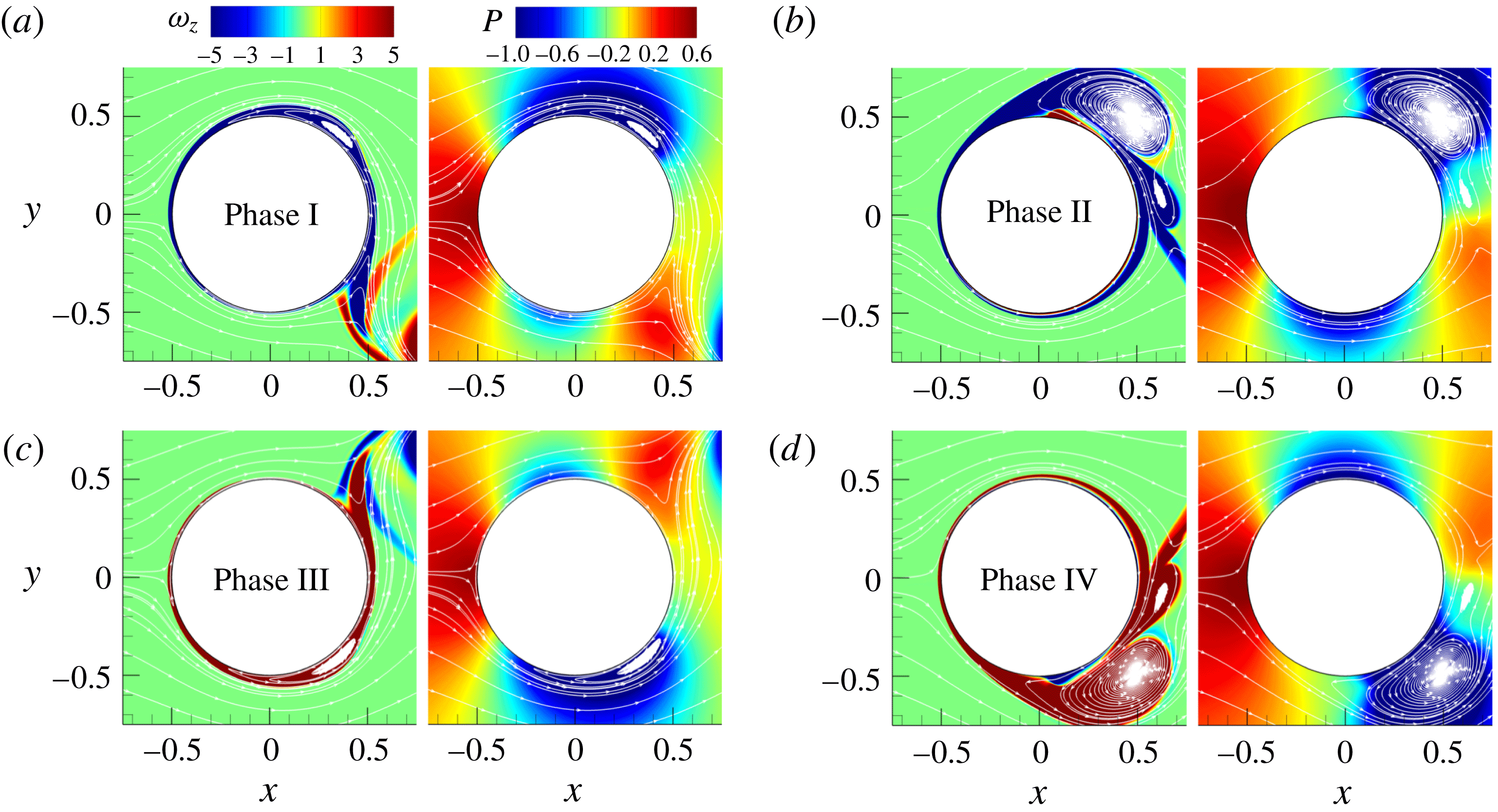
in the near-wall region at the end of each phase, denoted by dots in the sketch in table 3. The flow stabilizes due to rotation where the wall tangential velocity is aligned with the bulk flow (stable side) because the shear becomes smaller, while it is destabilized in the opposite case promoting instabilities (unstable side). The picture is complicated by the fact that the cylinder does not rotate with a constant angular velocity, but oscillates in the direction and magnitude. Figure 9(a) shows the end of phase I (point a) when
 $U_{\unicode[STIX]{x1D703}}^{wall}$
reaches its maximum value as the cylinder increases its angular velocity. The upper half of the flow near the cylinder wall, stabilized in the previous phase with favourable rotation, starts to destabilize due to the opposite rotation and generation of small-scale wall eddies, figure 9(a). At the lower half of the cylinder two counter-rotating wall-attached vortices are present in the near-wall region at the location previously occupied by the large vortex that is detached from the wall and convected downstream during phase I. Shiels & Leonard (Reference Shiels and Leonard2001) found the vortex to be formed on the stable side where the maximum shear occurs due to the co-existence of two vorticity layers with opposite signs. One is generated in the previous phase when the rotational direction was opposite and a new one is generated in the present phase. During phase II the newly formed wall-attached positive vorticity layer spreads to the upper half separating the existing negative-sign vorticity layer from the wall. At the same time, the lower part of the cylinder is stabilized with a laminar-like flow around the cylinder, figure 9(b). The change of rotational direction in phase III results in bursts of the boundary layer in the upper half of the cylinder leading to the formation of the main vortex away from the wall. The instabilities grow on the previously stable lower side resulting in the formation of the wall-attached vortex visible at the end of phase III, see figure 9(c). In phase IV the vortical structure that is formed on the unstable side grows, but stays attached to the wall as long as the rotation supports its growth. The stable side is not fully stabilized at the end of phase IV, as seen in figure 9(d). It is interesting to notice two different ways in which the main vortex is generated during phases I and II in the upper half and during phases III and IV in the lower half. In the first case (upper half) the main vortex is detached from the wall already in phase I. It grows away from the wall before it is shed downstream. In the second case the main vortex grows attached to the wall through phases III and IV before the change of the rotational direction causes its detachment from the cylinder and convection into the near wake. In the corresponding pressure fields the low-pressure region is determined by the presence of large-scale vortex structures at the end of phases II and IV, and by a high streamwise velocity at the top and bottom of the cylinder at the end of phases I and III, respectively. As the strength and position of the main vortex are not the same from cycle to cycle, the appearance and size of the low-pressure region vary between cycles. As shown below, this results in uneven amplitudes in the lift and drag coefficients.
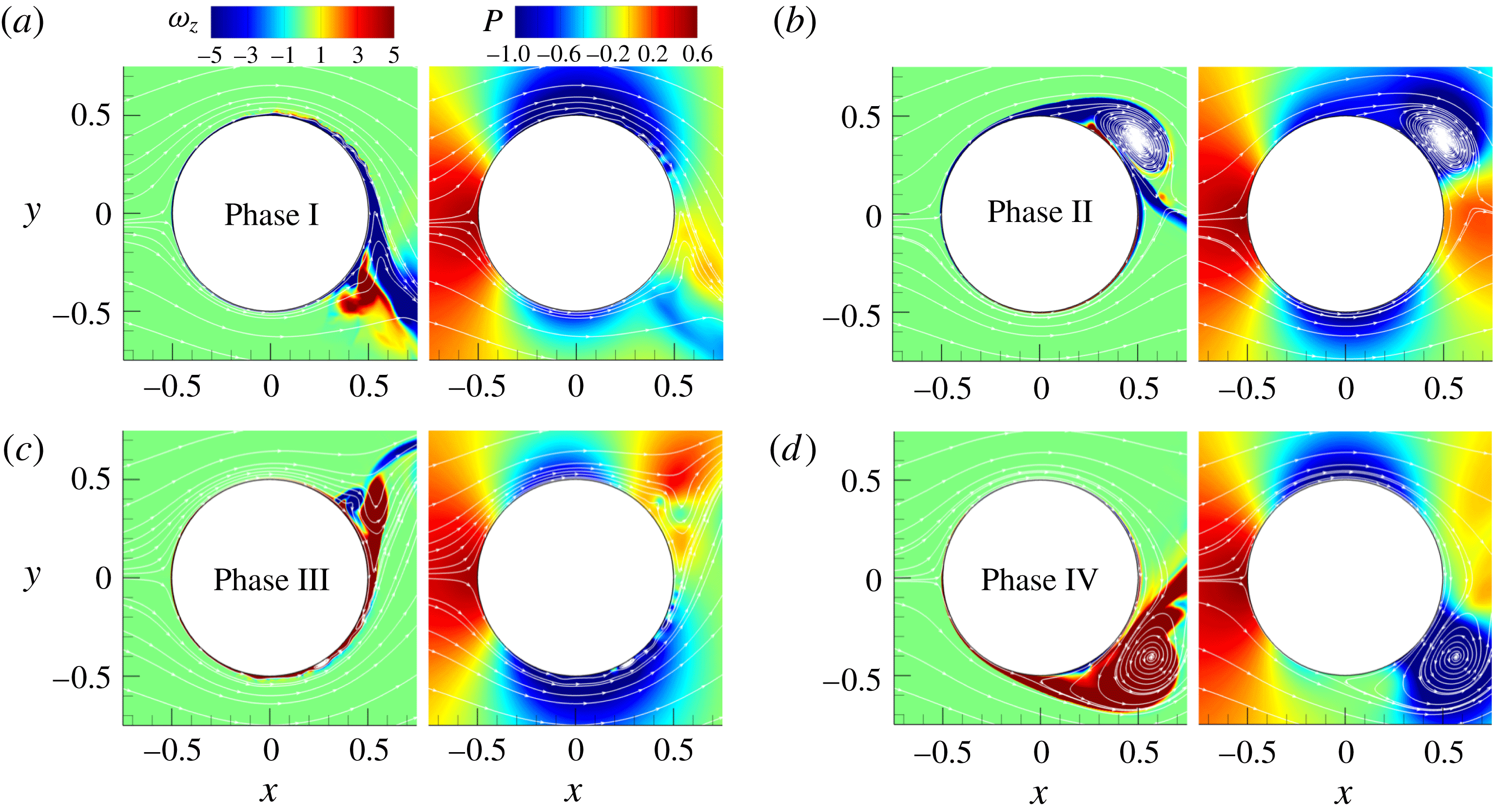
The increase of the rotational amplitude to 2 provides a more regular flow, figure 10. The negative-sign vorticity layer formed during phase I, see figure 10(a), grows into a large vortical structure during phase II, see figure 10(b). The wall-attached bubble of the opposite vorticity sign is formed at the end of phase II and grows rapidly at the beginning of phase III. The burst of the boundary layer that takes place at the beginning of phase III drags also the positive vorticity of the main vortex forming a multipole vortex structure. A similar dynamics is reported by Shiels & Leonard (Reference Shiels and Leonard2001) but for a much lower Reynolds number, where they observed a rapid growth of the multipole vortex structure triggered by separation, which is quickly pulled outside the boundary layer. Once the rotation changes its direction (phase III), the large-scale structure gets detached from the wall and convected downstream, as is visible in figure 10(c). The same mechanism leads to the formation of the main vortex during phases III and IV. The flow structures developed in phases III and IV are very similar in size and location to the vortices generated in phases I and II. The increase of the amplitude changes the positions of the attached vortices. While for
 $\unicode[STIX]{x1D6FA}=1$
the large wall-attached vortices migrate along the cylinder wall occasionally reaching the rear of the cylinder, for
 $\unicode[STIX]{x1D6FA}=2$
the attached vortices do not go further than
 $\unicode[STIX]{x1D703}=130^{\circ }$
(
 $\unicode[STIX]{x1D703}=180^{\circ }$
corresponds to the rear point) as they are quickly shed downstream. The changed position of the main vortex and its quick removal from the cylinder prevents the formation of large-scale separation in the wake which results in the disappearance of the separation bubble in the mean velocity field. The corresponding pressure fields show fewer differences in the distribution of the low-pressure zone for the same events as the flow becomes more regular. Stronger vortices result in a lower value of the pressure in the low-pressure region but at the same time there is a significant increase of the pressure in the rear.
Instantaneous fields of spanwise vorticity and pressure for
 $\unicode[STIX]{x1D6FA}2-f1$
.

Instantaneous fields of spanwise vorticity and pressure for
 $\unicode[STIX]{x1D6FA}3-f1$
.

An increase of the rotational amplitude to
 $\unicode[STIX]{x1D6FA}=3$
leads to a further enlargement of the wall-attached separation bubble visible in figure 11(a). The increase of the separation layer produces a larger and stronger wall-attached vortex. The flow becomes more regular as the stable size of the cylinder is further stabilized, figure 11(b). The flow structures are reduced to the main vortex with no other visible instabilities. The instantaneous vorticity fields in phases I and II are almost identical to the fields in phases III and IV, respectively, with flipped top and bottom halves indicating a significant reduction in turbulence-induced fluctuations. The position of the main vortex, a moment before it is shed away from the wall, is moved further away from the centreline towards the top and bottom positions, while the pressure in the low-pressure region gets lower. There are no other significant differences from the previous case of
 $\unicode[STIX]{x1D6FA}=2$
.
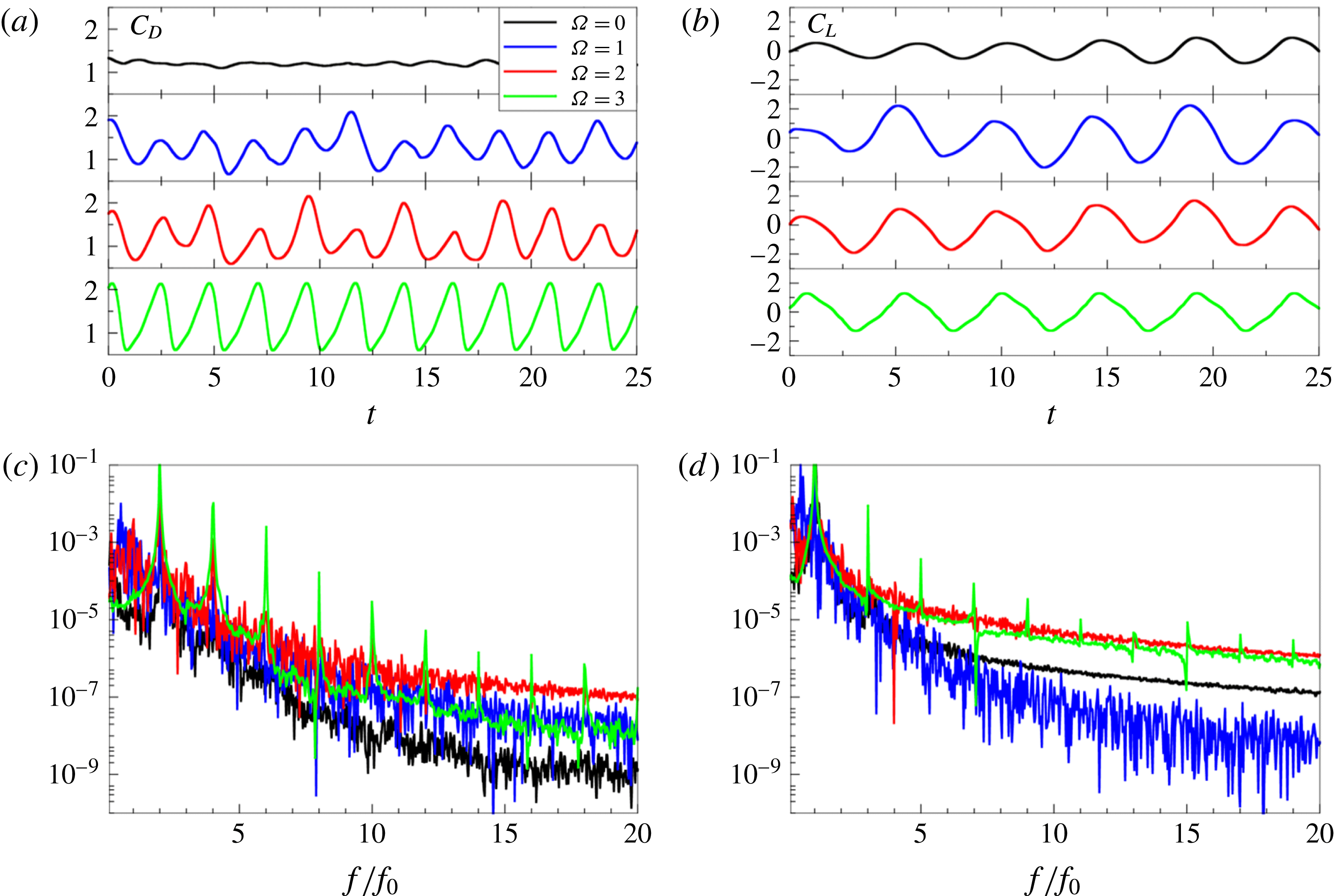
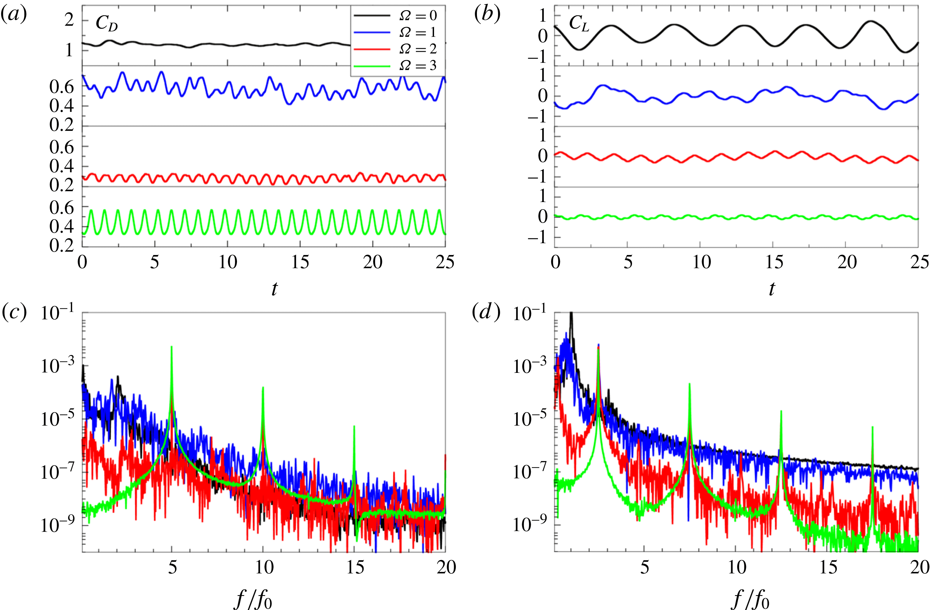
(a) Drag and (b) lift coefficient for frequency
 $f=1$
as well as their power spectra shown in (c), (d), respectively.

Interestingly, the change of the flow topology does not influence much the mean values of the drag coefficient. However, the histories of the drag and lift coefficients, shown in figure 12(a,b), reveal the strong impact of the rotation on the instantaneous values of
 $C_{D}$
and
 $C_{L}$
, which is in agreement with the results for lower Reynolds numbers (Cheng et al.
Reference Cheng, Chew and Luo2001; Du & Dalton Reference Du and Dalton2013). The amplitudes in both signals increase compared to the non-rotating case. High
 $\unicode[STIX]{x1D6FA}$
values lead to a decrease of the irregularities in both signals, as seen in figure 12(a,b). While for
 $\unicode[STIX]{x1D6FA}2-f1$
some low-frequency modulations of the signal can still be traced, the
 $\unicode[STIX]{x1D6FA}3-f1$
case produces almost perfect periodical oscillations of both
 $C_{D}$
and
 $C_{L}$
with a constant value of the oscillation amplitude (lock-on). Contrary to
 $C_{D}$
, the amplitude in the
 $C_{L}$
signal decreases for high
 $\unicode[STIX]{x1D6FA}$
. As already mentioned above, the time histories of
 $C_{D}$
and
 $C_{L}$
and their spectral analysis indicates that the lock-on phenomena, i.e. the synchronization of rotation dynamics and vortex shedding resulting in one dominant spectral peak with the frequency of rotation, is most pronounced at high
 $\unicode[STIX]{x1D6FA}$
with the flow becoming quasi-laminar and almost perfectly periodic. The low-frequency modulation effects were also seen in the 2-D simulations of Choi et al. (Reference Choi, Jeon and Kim2008), who showed that the modulation was related to the vortex-merging process in the wake further downstream. It has been reported in the literature (Mahfouz & Badr Reference Mahfouz and Badr2000) that, below a threshold value of the forcing amplitude, the lock-on region diminishes to zero. Further, below, we compare all our regimes with the results of D’Adamo, Godoy-Diana & Wesfreid (Reference D’Adamo, Godoy-Diana and Wesfreid2011) at
 $Re=100$
and Cheng et al. (Reference Cheng, Chew and Luo2001) at
 $Re=200$
indicating that only for
 $\unicode[STIX]{x1D6FA}=3$
and all
 $f$
is the wake dynamics quasi-laminar close to the cylinder wall and synchronized with the rotation of the cylinder further downstream, see figure 19.
3.3 Forcing frequency
$f=2.5$

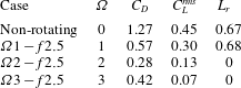
The increase of the rotational frequency to 2.5 leads to a significant reduction of the mean drag coefficient as well as the root mean square value of the lift coefficient, see table 4. The mean drag coefficient is reduced by almost
 $80\,\%$
for amplitude
 $\unicode[STIX]{x1D6FA}=2$
, while for
 $\unicode[STIX]{x1D6FA}=1$
and
 $3$
these values are
 $55\,\%$
and
 $67\,\%$
, respectively. Tokumaru & Dimotakis (Reference Tokumaru and Dimotakis1991), Shiels & Leonard (Reference Shiels and Leonard2001) and Du & Dalton (Reference Du and Dalton2013) reported a drop in the drag coefficient for frequencies larger than the natural frequency. Du and Dalton found the largest drop of
 $57\,\%$
for
 $f=2.5$
and
 $\unicode[STIX]{x1D6FA}=2$
for several tested frequencies. Indeed, we observe a solid trend of further drag reduction when the Reynolds number is increased.
Mean streamwise velocity and pressure fields for
 $f=2.5$
and different amplitudes.

Mean drag coefficient (
 $C_{D}$
), root mean square of the lift coefficient (
 $C_{L}^{rms}$
) and length of the recirculation zone (
 $L_{r}$
) for different rotational amplitudes for forcing frequency
 $f=2.5$
.
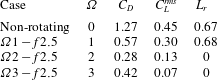
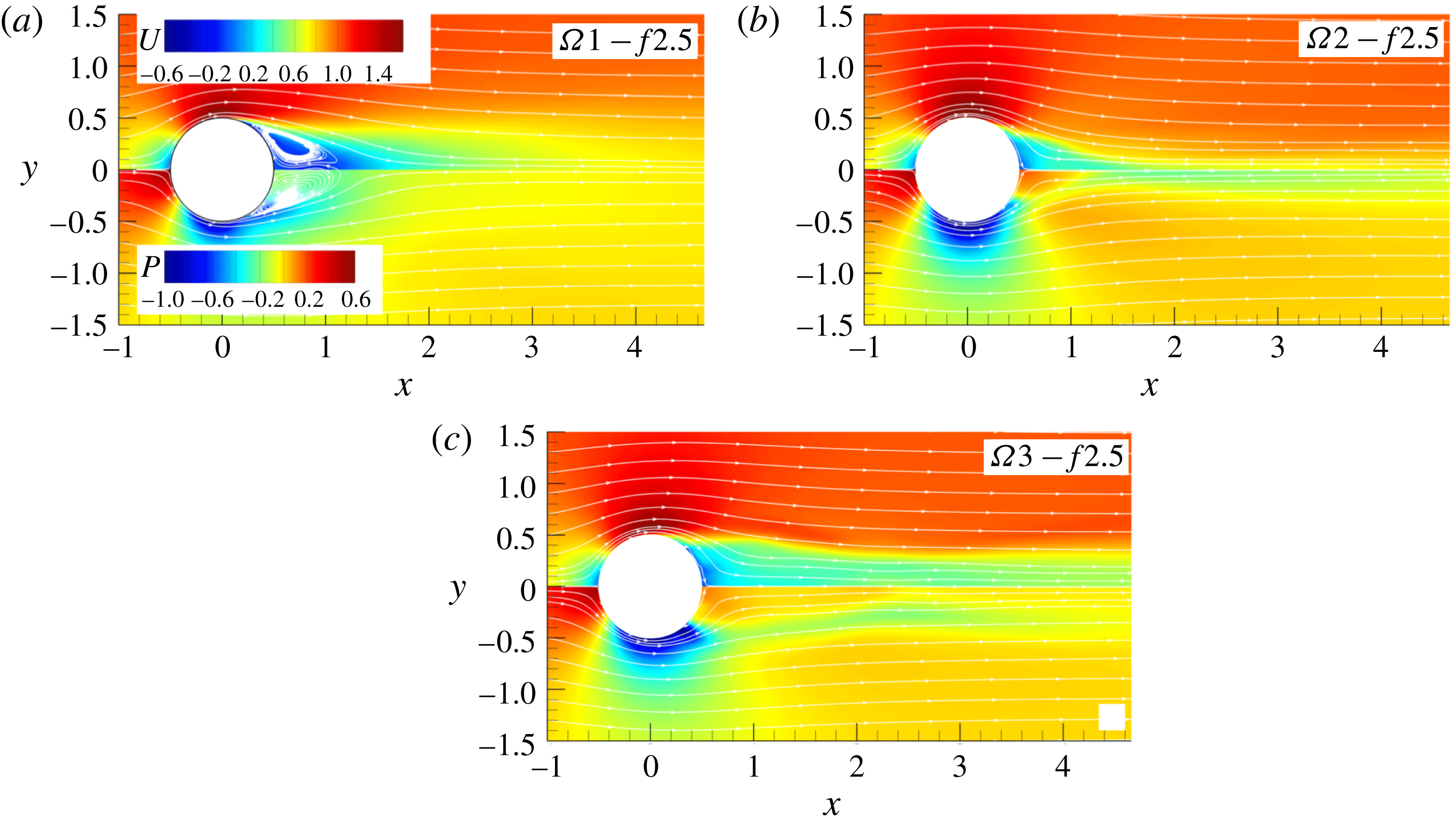
Figure 13 shows the mean fields of the streamwise velocity and pressure for three forcing amplitudes. As in the case for
 $f=1$
, the main separation bubble disappears for amplitudes
 $\unicode[STIX]{x1D6FA}=2$
and 3 while a reduced bubble is still present for
 $\unicode[STIX]{x1D6FA}=1$
. The mean velocity fields do not show much variation from the corresponding fields for
 $f=1$
, while the mean pressure shows remarkable differences. The main difference from the previous case appears especially in the rear of the cylinder where the pressure dramatically increases for all
 $\unicode[STIX]{x1D6FA}$
. It is interesting to note that this pressure increase is the highest for
 $\unicode[STIX]{x1D6FA}=2$
, while for
 $\unicode[STIX]{x1D6FA}=3$
the low-pressure zones at the top and bottom of the cylinder extend further towards the centreline.
Instantaneous fields of spanwise vorticity for three amplitudes and
 $f=2.5$
.

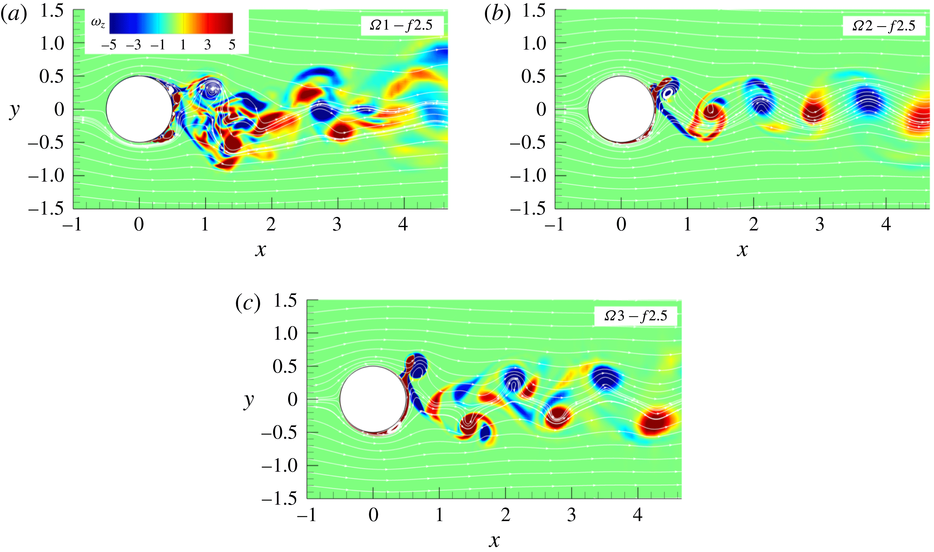
The most striking difference in the wake organization, shown in figure 14, is a high sensitivity of the wake structures to the imposed amplitudes compared to the previous case when
 $f=1$
. While for
 $f=1$
different
 $\unicode[STIX]{x1D6FA}$
produce the same wake pattern, for the increased frequency each amplitude produces a different wake structure. The lowest amplitude,
 $\unicode[STIX]{x1D6FA}=1$
, results in a flow that is much more irregular and unstable compared to the corresponding case with
 $f=1$
. The two competing frequencies, the natural and the imposed rotational frequency, produce near-wall eddies at both halves of the cylinder simultaneously which coalesce and evolve into a single large vortex. The cylinder releases two vortices per cycle of approximately equal size, one vortex per half-cycle. The multipole vortical structures interact in the wake once they detached from the wall, leading to a good deal of cancellation of the opposite-sign vorticity. In the process these vortices become less distinct and after a distance of
 $3D$
downstream no coherent structures are visible. The wake organization resembles to some extend the mode III defined by Tokumaru & Dimotakis (Reference Tokumaru and Dimotakis1991). By increasing the amplitude to 2, the wake synchronizes again to the cylinder rotation and becomes more regular, figure 14(b). The increased rotational amplitude is now strong enough to periodically stabilize the boundary layer on one half of the cylinder. The cylinder again produces one vortex per cycle. However, what makes this case interesting is the one-column organization of the wake, making it significantly narrower compared to all previous wake patterns. While the way the main vortices are generated in the shear layer is not much different from
 $f=1$
case, the higher frequency reduces the size of the vortices ejected from the wall as they have less time to grow supported by rotation. A further increase of the amplitude to
 $\unicode[STIX]{x1D6FA}=3$
, restores the two-column wake organization, figure 14(c). The main vortex increases in size due to thickening of the boundary layer out of which the main vortex is generated. The wake widens as the main vortices are displaced laterally due to a strong stream of fluid generated by rotation but it is still narrow compared to the corresponding case with
 $f=1$
.
Instantaneous fields of spanwise vorticity and pressure for
 $\unicode[STIX]{x1D6FA}1-f2.5$
.

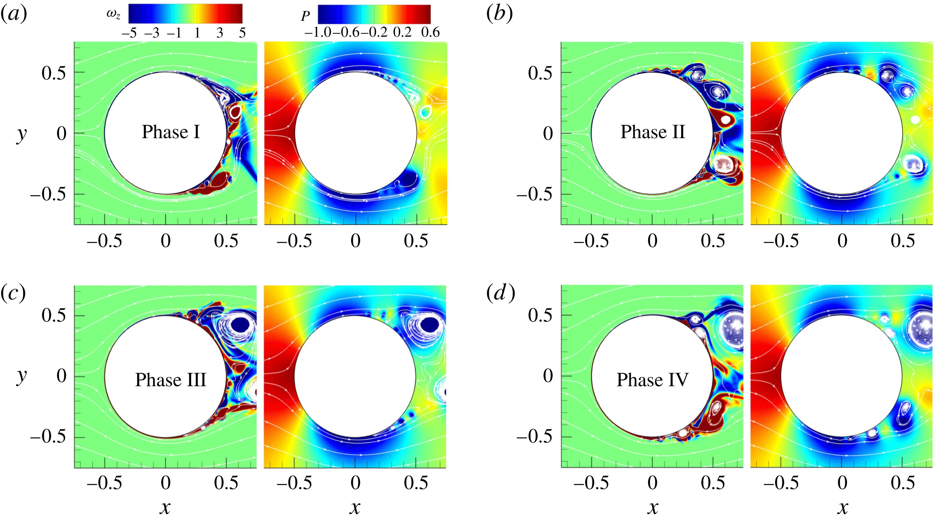
Figure 15 shows the instantaneous vorticity fields in the near-wall region at the end of the four phases. At the end of phase I, figure 15(a) reveals a large number of small-scale structures contrary to the case
 $\unicode[STIX]{x1D6FA}1-f1$
where the corresponding flow field contains the main vortex and only a very few small eddies. The change of the rotational direction at the beginning of phase I leads to the formation of a vortex at the lower half of the cylinder (stable side) that grows as the rotation speed increases. The upper half (unstable side) is populated by two counter-rotating vortices that are attached to the wall. This is another profound difference compared with the lower-frequency case where the unstable side was without visible vortical structures at the end of phase I. During phase II the vortex in the lower half moderately grows and stays close to the wall. At the same time the counter-rotating vortices on the other side detached from the wall as new vortices appear in the wall region of the unstable side, figure 15(b). The change of the rotational direction in phase III causes a coalescence of small vortical structures in the upper half (now stable side) that results in the formation of a new main vortex visible at the end of phase III, figure 15(c). In the meantime, the large vortex in the lower half is detached from the wall and convected downstream. The phase III ends with two dominant vortical structures at the bottom and top of the cylinder, both detached from the wall, but there are also a large number of small-scale vortices present in the flow. During phase IV, new wall-attached eddies appear at both halves of the cylinder. It is interesting to notice that the main vortex is frequently formed away from the wall as the separation bubble is detached from the wall by the opposite-sign vorticity layer generated by the rotation. This can be seen in the upper half during phases I and II (figure 15
a,b), and in the lower half in phases III and IV (figure 15
c,d). There are a very few locations where the low-pressure zones are attached to the wall as the vortices responsible for the low-pressure regions are efficiently removed away from the wall. Additional reduction of the low-pressure zone comes from the diminishing of the vortices size.
The increase of the forcing amplitude to
 $\unicode[STIX]{x1D6FA}=2$
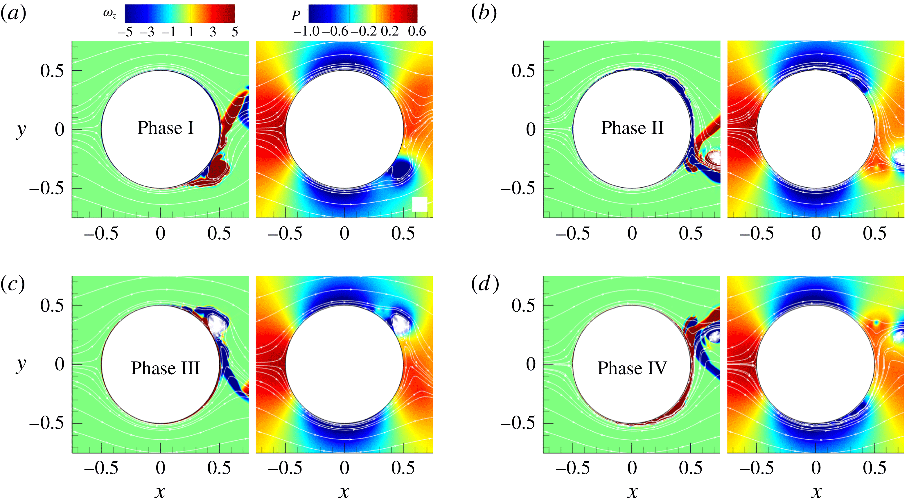
dramatically reduces the number of small-scale structures and consequently makes the flow pattern more regular. The end of phase I, shown in figure 16(a), is characterized by a large vortex that is attached to the wall and located on the stable side (lower half) with no visible eddies on the unstable side (upper half). The opposite-sign vorticity layer is present at the end of phase I in the stable region between the main vortex and the wall. During phase II this layer grows and efficiently removes the main vortex from the wall and drags it downstream while on the unstable side a wall-attached narrow separation bubble is formed, figure 16(b). The same scenario repeats during phase III but on the upper side. The separation bubble evolves into an eddy during phase III and it is removed quickly by the fast growing opposite-sign vorticity layer, figure 16(c). The phase IV ends with an almost identical vorticity field as in phase II but with exchanged upper and lower sides. The pressure field shows an increase of the pressure at the rear of the cylinder while the vortex-generated low-pressure region reduces further in size.
Instantaneous fields of spanwise vorticity and pressure for
 $\unicode[STIX]{x1D6FA}2-f2.5$
.

As the amplitude further increases to
 $\unicode[STIX]{x1D6FA}=3$
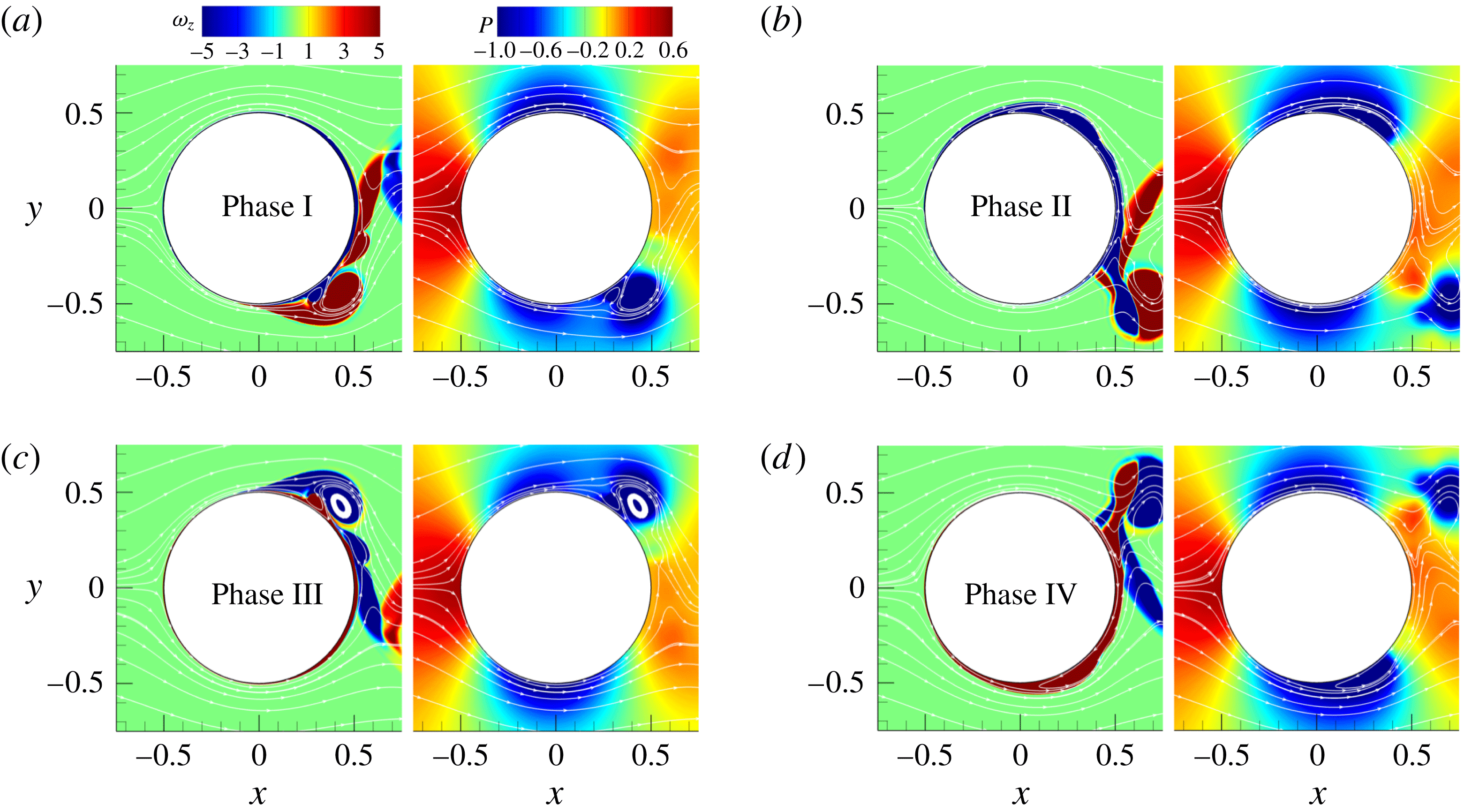
, figure 17, the main vortex formed on the stable side is already detached from the wall at the end of phase I as the new vortex with opposite vorticity sign appears between the wall and the large vortical structure. The wall-attached separation bubble considerably increases in size during phase II compared to
 $\unicode[STIX]{x1D6FA}=2$
and it evolves into the main vortex once the rotation changes direction. At the end of phase II and IV large vortical structures that are generated in the wall vicinity are efficiently removed away from the wall. This is visible in the pressure field as well. The phase II ends up with a large low-pressure zone located in the region occupied by the wall-attached separation bubble which extends further down to the centreline. The low-pressure zone also exists on the opposite side of the cylinder generated by a large rotational amplitude.
Instantaneous fields of spanwise vorticity and pressure for
 $\unicode[STIX]{x1D6FA}3-f2.5$
.

The evolution in time of
 $C_{D}$
and
 $C_{L}$
, figure 18, shows very different patterns from those presented in figure 12 for
 $f=1$
. Contrary to the
 $f=1$
case where the amplitudes of the
 $C_{D}$
and
 $C_{L}$
oscillations increase with rotation, the higher frequency (
 $f=2.5$
) results in a reduced amplitude of the
 $C_{D}$
and
 $C_{L}$
signals for all three forcing amplitudes, especially for the case
 $\unicode[STIX]{x1D6FA}2-f2.5$
. As was the case with a forcing frequency
 $f=1$
, the drag and lift coefficients show a more regular oscillating pattern as the forcing amplitude increases. The
 $C_{D}$
and
 $C_{L}$
signals get nearly sinusoidal already for a forcing amplitude 2, with a modulation in the
 $\unicode[STIX]{x1D6FA}2-f2.5$
case. For the higher amplitude
 $\unicode[STIX]{x1D6FA}=3$
, the
 $C_{L}$
spectrum corresponds to a quasi-laminar flow and has a dominant peak at
 $f=2.5$
as opposed to the lower amplitudes still having a lower-frequency signal. Thus, we can point again to the lock-on for high-amplitude modulations with
 $\unicode[STIX]{x1D6FA}=3$
and
 $f=2.5$
.
(a) Drag and (b) lift coefficient for frequency
 $f=2.5$
as well as their power spectra shown in (c), (d), respectively.

3.4 Forcing frequencies
$f=3$
,
$4$
and
$5$


The results for forcing frequencies,
 $f=3{-}5$
, are discussed together since they do not differ much from the
 $f=2.5$
case described above. Even a small increase of the frequency, from
 $f=2.5$
to
 $3$
, leads to a further reduction in the size of vortical structures. The mechanism described earlier applies here as well. As the rotational frequency is increased, the time needed for vortices in the shear layer to grow is reduced, leading to the decrease of the main vortex size for all three tested amplitudes. The wake organization for
 $f=3$
stays very similar to the
 $f=2.5$
case. A further increase of the rotational frequency (
 $f=4$
and 5) does not bring significant change in the overall flow dynamics. The reduction in the vortex size with increasing frequency is visible for all amplitudes although it is less pronounced for
 $\unicode[STIX]{x1D6FA}=2$
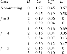
. The impact of the high frequency on the drag coefficient is discussed in the next section. Table 5 summarizes the values of
 $C_{D}$
for the above discussed higher frequencies for all three amplitudes.
Mean drag coefficient (
 $C_{D}$
) and length of the recirculation zone (
 $L_{r}$
) for different rotational amplitudes
 $\unicode[STIX]{x1D6FA}$
and forcing frequencies
 $f=3$
,
 $4$
and
 $5$
.
3.5 Lock-on diagram
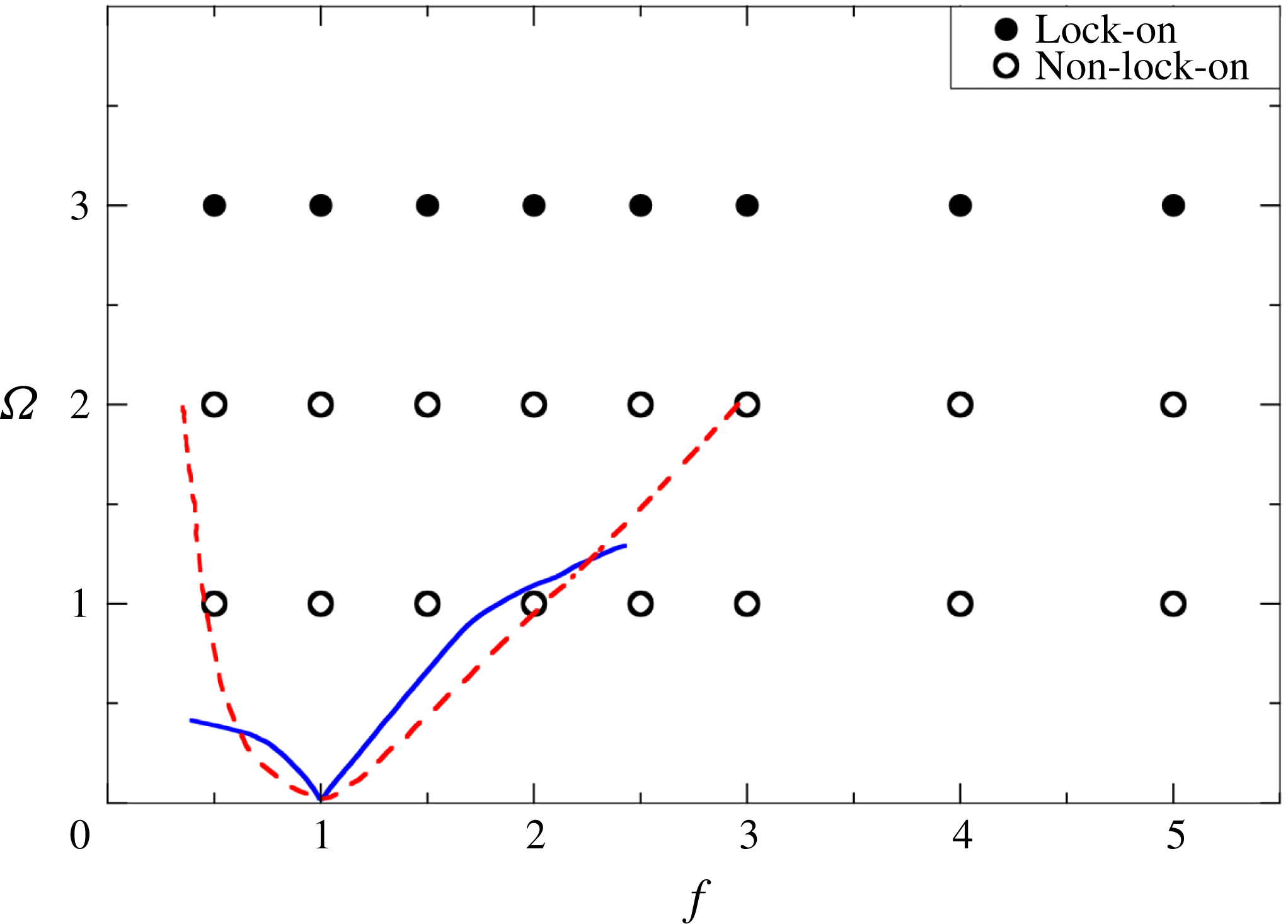
Figure 19 shows a lock-on map for the explored set of forcing frequencies and amplitudes based on the power spectra of the lift and drag coefficients. The lock-on regime is characterized by a single peak in the
 $C_{D}$
and
 $C_{L}$
power spectra while the non-lock-on regime is denoted when, apart from the dominant peak at the forced frequency, there is an additional peak at another frequency or some broadband dynamics due to small-scale vortices. Thus, the criterion for the lock-on is the absence of low-frequency modulation due to the vortical dynamics downstream and the laminarization of the boundary layer near the cylinder due to strong enough rotation. A significant increase of
 $Re$
number in the present study compared to the previous work leads to the observation of the lock-on regime in the sense defined above only for
 $\unicode[STIX]{x1D6FA}=3$
(shown with filled circles in figure 19). The results of previous research on laminar flows reported by D’Adamo et al. (Reference D’Adamo, Godoy-Diana and Wesfreid2011) for
 $Re=100$
and Cheng et al. (Reference Cheng, Chew and Luo2001) for
 $Re=200$
are also presented in figure 19 showing a strong dependence on the frequency of oscillations while for the present case the governing parameter is the amplitude. However, our results are consistent with LES spectra presented by Du & Dalton (Reference Du and Dalton2013) for
 $Re=1.5\times 10^{4}$
and
 $\unicode[STIX]{x1D6FA}=2$
.
The diagram in
 $f-\unicode[STIX]{x1D6FA}$
space where filled circles correspond to the lock-on regime while a hollow circle denotes the non-lock-on regime for the present set of simulations. The blue solid and red dashed curves show the boundaries between these two regimes for
 $Re=100$
and
 $200$
obtained by Cheng et al. (Reference Cheng, Chew and Luo2001) and D’Adamo et al. (Reference D’Adamo, Godoy-Diana and Wesfreid2011).

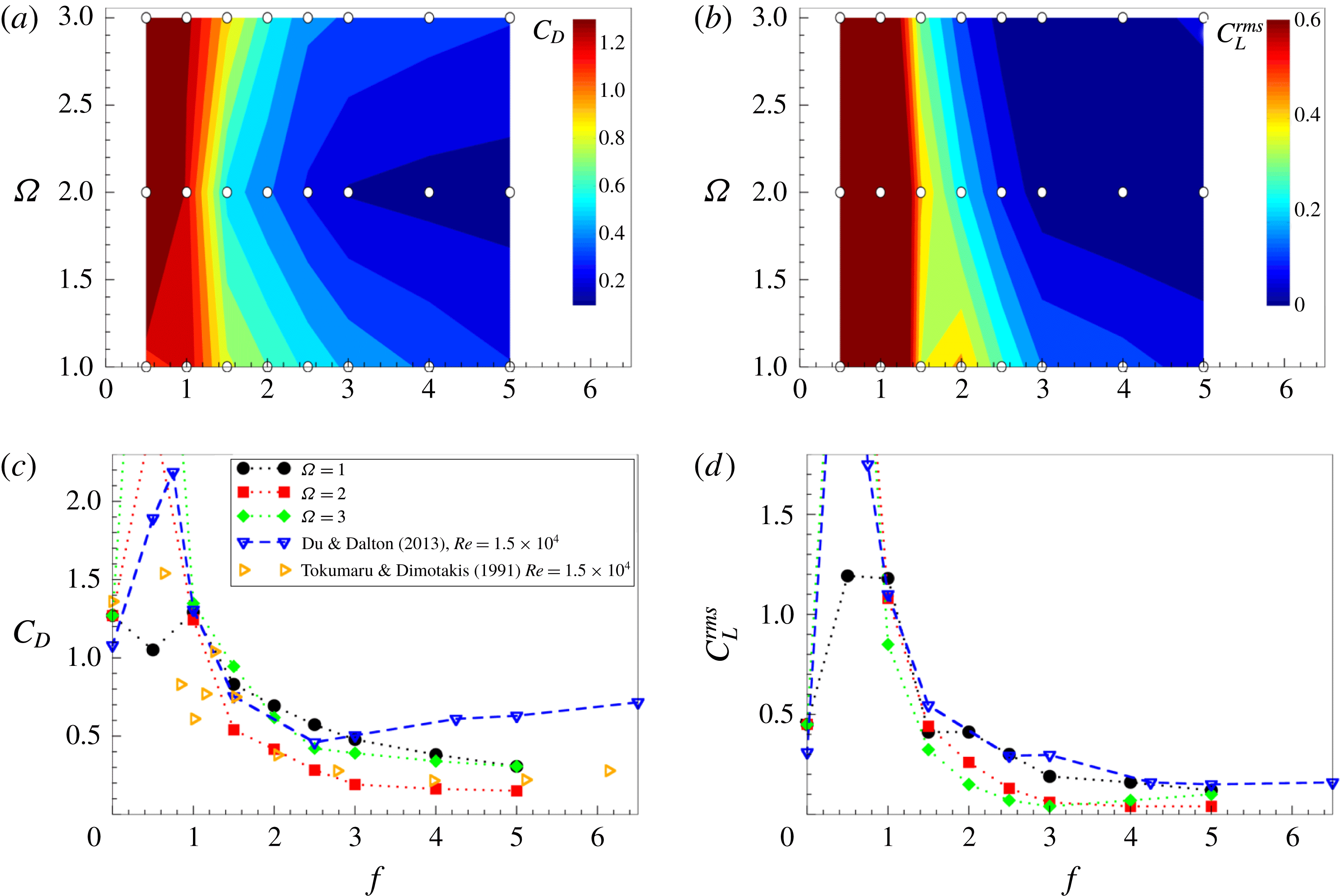
(a,b) Drag coefficient and root mean square of the lift coefficient for different rotational frequencies and amplitudes obtained from simulations at
 $Re=1.4\times 10^{5}$
. White points show the simulated cases. (c,d) The same data compared to data from the literature at lower Reynolds number for
 $\unicode[STIX]{x1D6FA}=2$
(Tokumaru & Dimotakis Reference Tokumaru and Dimotakis1991; Du & Dalton Reference Du and Dalton2013).

4 Drag reduction mechanism due to rotary oscillations
We now discuss the drag reduction mechanism for the forcing frequency
 $f=2.5$
and higher, as well as its absence for relatively low
 $f$
. Figure 20 shows how the drag coefficient varies with the rotational frequency
 $f$
for three different amplitudes. A significant reduction occurs for
 $f>1$
. With a further increase of frequency,
 $C_{D}$
continues to decrease but at a slower pace. There is a notable difference in the drag reduction for different rotational amplitudes. The highest decrease of
 $C_{D}$
occurs for
 $\unicode[STIX]{x1D6FA}=2$
and the lowest for
 $\unicode[STIX]{x1D6FA}=1$
, while for
 $\unicode[STIX]{x1D6FA}=3$
it falls in between, but closer to the
 $C_{D}$
values for
 $\unicode[STIX]{x1D6FA}=1$
.
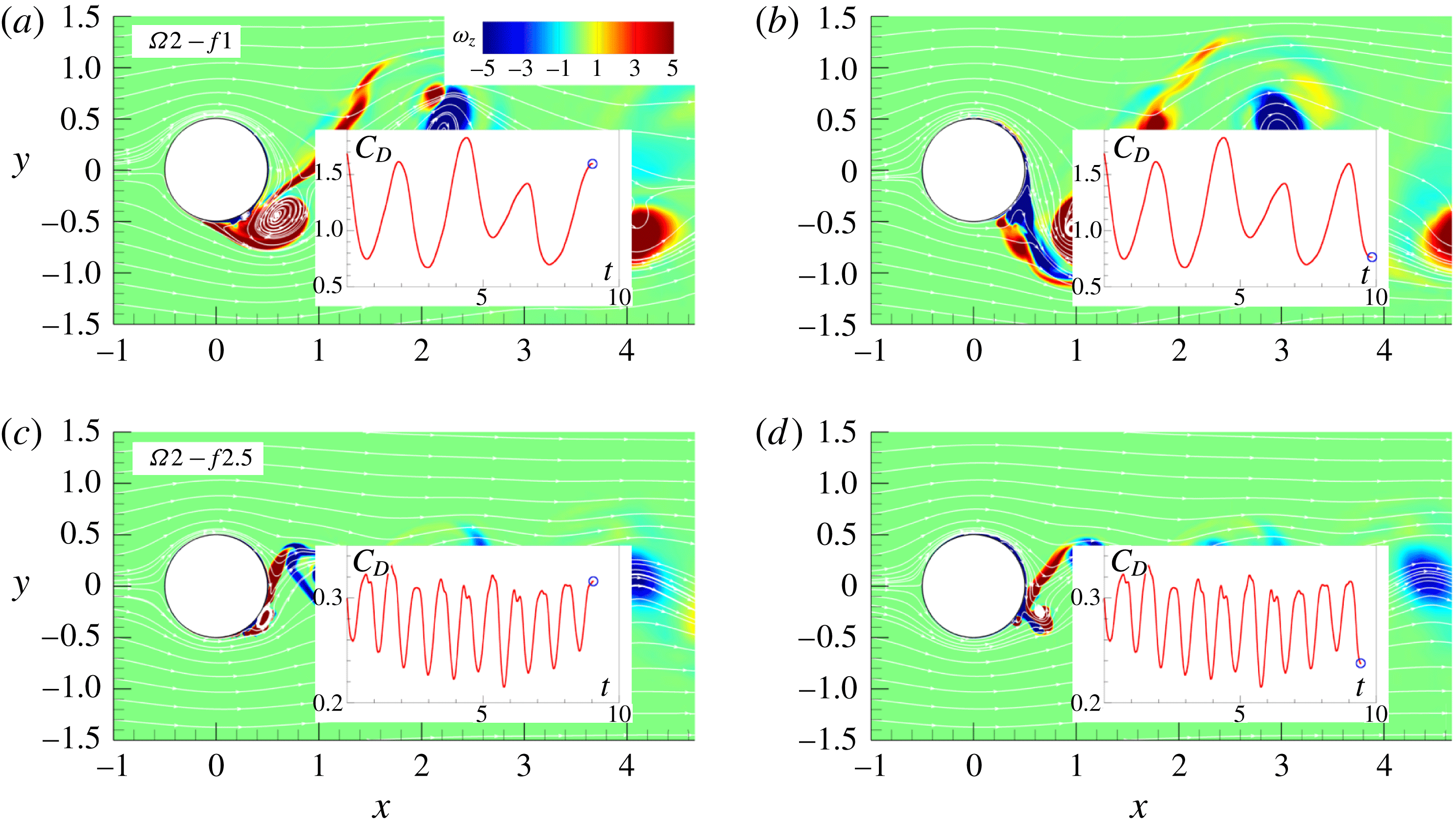
As at high Reynolds number
 $C_{D}$
is governed mainly by the pressure force, the key to understanding the drag reduction mechanism is to understand the way the low-pressure zone is generated and distributed in the region near the cylinder wall. The instantaneous vorticity fields shown in the previous sections reveal that the dynamics of the near-wall vortices has a profound effect on the low-pressure region in the wake. At low frequencies the flow features a set of main vortices which are amplified in strength and size and formed in the shear layer. An inspection of the instantaneous values and time variations of the drag coefficient and the corresponding vorticity fields for the case
 $\unicode[STIX]{x1D6FA}2-f1$
shown in figure 21(a) reveals that
 $C_{D}$
grows to its maximum at the end of phases II and IV in which the main vortex, enhanced by rotation, grows to its maximum size either in the cylinder wall vicinity or attached to the wall (see also figure 10
b,d). The value of
 $C_{D}$
begins to decrease when the main vortex starts to move away from the wall during phases I and III. The drag coefficient reaches its minimum when the main vortex is shed downstream, while the new main vortex is still not formed, figure 21(b). Although the
 $C_{D}$
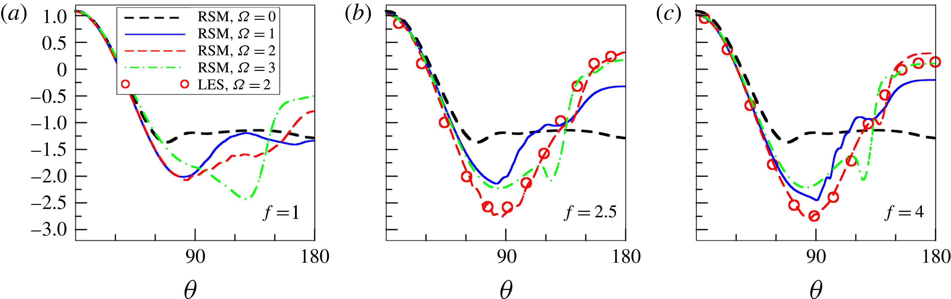
signal is very different from the non-rotating case, the mean drag coefficient does not change much. The distribution of the mean pressure coefficient
 $C_{p}=2(P-P_{\infty })/\unicode[STIX]{x1D70C}U_{\infty }^{2}$
around the cylinder wall is shown in figure 22, where
 $P_{\infty }$
denotes the pressure far from the cylinder. For
 $\unicode[STIX]{x1D6FA}=1$
, the mean pressure over the circumferential segments from
 $\unicode[STIX]{x1D703}=120^{\circ }$
to
 $180^{\circ }$
is not changed much compared to the non-rotating case, where
 $\unicode[STIX]{x1D703}=180^{\circ }$
corresponds to the rear point. As the rotational amplitude increases to
 $\unicode[STIX]{x1D6FA}=2$
and
 $\unicode[STIX]{x1D6FA}=3$
the minimum pressure in the low-pressure region during phases II and IV becomes lower due to rotational enhancement of the main vortex, see figures 10(b,d) and 11(b,d). The low-pressure region for
 $\unicode[STIX]{x1D6FA}=2$
and
 $\unicode[STIX]{x1D6FA}=3$
is located around
 $\unicode[STIX]{x1D703}=135^{\circ }$
and
 $120^{\circ }$
, respectively, reflecting the position of the main vortex at the end of phases II and IV. The higher rotational amplitude completely suppresses flow recirculation. As a result, at the end of phases I and III the pressure is much higher at the rear part of the cylinder wall, see figures 10(b,d) and 11(b,d), as also visible in figure 22. The absolute values of both the minimum and maximum mean pressure increase but the resulting drag coefficient does not differ much from the mean non-rotating value.
Instantaneous vorticity fields and short-time variation of the drag coefficient for (a,b)
 $\unicode[STIX]{x1D6FA}2-f1$
and (c,d)
 $\unicode[STIX]{x1D6FA}2-f2.5$
.

Distribution of the mean pressure coefficient
 $C_{p}$
around the cylinder wall for
 $f=1$
,
 $2.5$
and
 $4$
. Symbols show LES results for
 $\unicode[STIX]{x1D6FA}2-f2.5$
and
 $\unicode[STIX]{x1D6FA}2-f4$
.

With the increase in
 $f$
, a significant drag reduction occurs when the rotational frequency
 $f$
reaches 2.5. The main flow feature at this frequency is a smaller size of the rotation-enhanced vortex on the unstable side due to a shorter time available for the vortex to grow. As for
 $f=1$
, the main vortex is formed in the vicinity of the wall at the end of phases II and IV but compared to the
 $\unicode[STIX]{x1D6FA}1-f1$
case it is removed faster from the wall and shed downstream, resulting in the absence of a wall-adjacent large low-pressure zone behind the cylinder. Figure 15 shows the pressure fields that have a few small low-pressure regions, mostly detached from the cylinder. This is a very different picture from the pressure field observed in the
 $\unicode[STIX]{x1D6FA}1-f1$
case (figure 9). The reduction of the low-pressure zone attached to the wall results in a significant 55 % drop in
 $C_{D}$
. Higher rotational amplitudes
 $\unicode[STIX]{x1D6FA}=2$
and
 $3$
make the flow more regular with fewer or almost no small-scale structures. The increase of
 $\unicode[STIX]{x1D6FA}$
generates a sufficiently strong opposing layer of vorticity to suppress instabilities in the boundary layer of the stable side (see the inset in figure 8
b). Now, the main vortex is not formed from an initial wall-attached eddy or by coalescence of small-scale structures generated in the near-wall region, but out of a narrow wall-attached separation bubble. While the main vortex is formed on one side of the cylinder, the opposite side is void of vortices and the fluid smoothly passes over the cylinder. The efficient supply of momentum to the rear region of the cylinder further increases the pressure in this region. Figures 16 and 17 reveal that the low-pressure zone is mainly located at the top and bottom of the cylinder, whereas behind the cylinder the pressure increases. This produces a further reduction of
 $C_{D}$
which for the case
 $\unicode[STIX]{x1D6FA}2-f2.5$
reaches a dramatic
 $78\,\%$
. Figure 21(c,d) confirms that the local maximum and minimum in the drag coefficient signal are related to the position and size of the main vortex. The maximum tested amplitude (
 $\unicode[STIX]{x1D6FA}=3$
) produces a larger wall-attached separation bubble which evolves into the main vortex. Consequently, the low-pressure zone at the top and bottom of the cylinder expands towards the centreline region at the back of the cylinder as shown in figure 17. This produces lower drag reduction (67 %) compared to the case with
 $\unicode[STIX]{x1D6FA}=2$
.
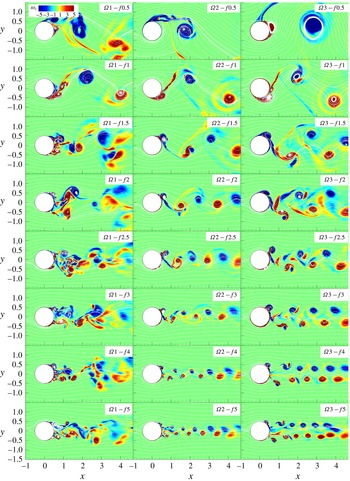
Instantaneous spanwise vorticity and streamlines for all cases considered.

Figure 22(b) shows the distribution of the mean pressure coefficient along the wall for
 $f=2.5$
. The main difference for two rotational frequencies occurs in the rear region from
 $140^{\circ }$
to
 $180^{\circ }$
. The higher frequency produces significantly higher pressure at the rear of the cylinder for all rotational amplitudes. As the time for growth of the tangential velocity in the boundary layer is reduced for higher frequency, the boundary layer in the rear is much thinner. In addition, the higher frequency leads to a reduction of the main vortex and its fast removal away from the wall. These effects of higher frequency result in a higher value of pressure in the rear part. The dip in the pressure that occurs around
 $120^{\circ }$
in the
 $\unicode[STIX]{x1D6FA}3-f2$
case reflects the wall-attached local separation bubble responsible for the increase of
 $C_{D}$
compared to the maximum drag reduction observed for
 $\unicode[STIX]{x1D6FA}=2$
. We can conclude that the reduction of the wall-attached low-pressure zone, resulting from the smaller size of the main vortex and its efficient removal from the wall in combination with lower values of the wall-tangential velocity in the boundary layer for
 $f=2.5$
, lead to a significant drag reduction that occurs for
 $\unicode[STIX]{x1D6FA}=2$
.
As noted above, figure 20,
 $C_{D}$
continues to decrease with a further increase of the rotational frequency beyond
 $f=2.5$
but at a slower rate. The reduction of the main vortex size with the increase of
 $f$
is visible in the instantaneous vorticity fields at different amplitudes and frequencies. Figure 23 clearly demonstrates that the drag reduction is related to the weakening of the main vortex generated in the initial shear layer and its efficient removal from the cylinder wall. The same figure shows why the rotational amplitude
 $\unicode[STIX]{x1D6FA}=2$
is optimal for the drag reduction: the amplitude
 $\unicode[STIX]{x1D6FA}=1$
is too weak to stabilize the flow at the stable side and to diminish the main separation bubble in the wake, but
 $\unicode[STIX]{x1D6FA}=3$
produces a thick separation layer attached to the cylinder wall in the rear region that leads to the formation of the main vortex which exceeds in size the main vortex in the cases with
 $\unicode[STIX]{x1D6FA}=2$
.
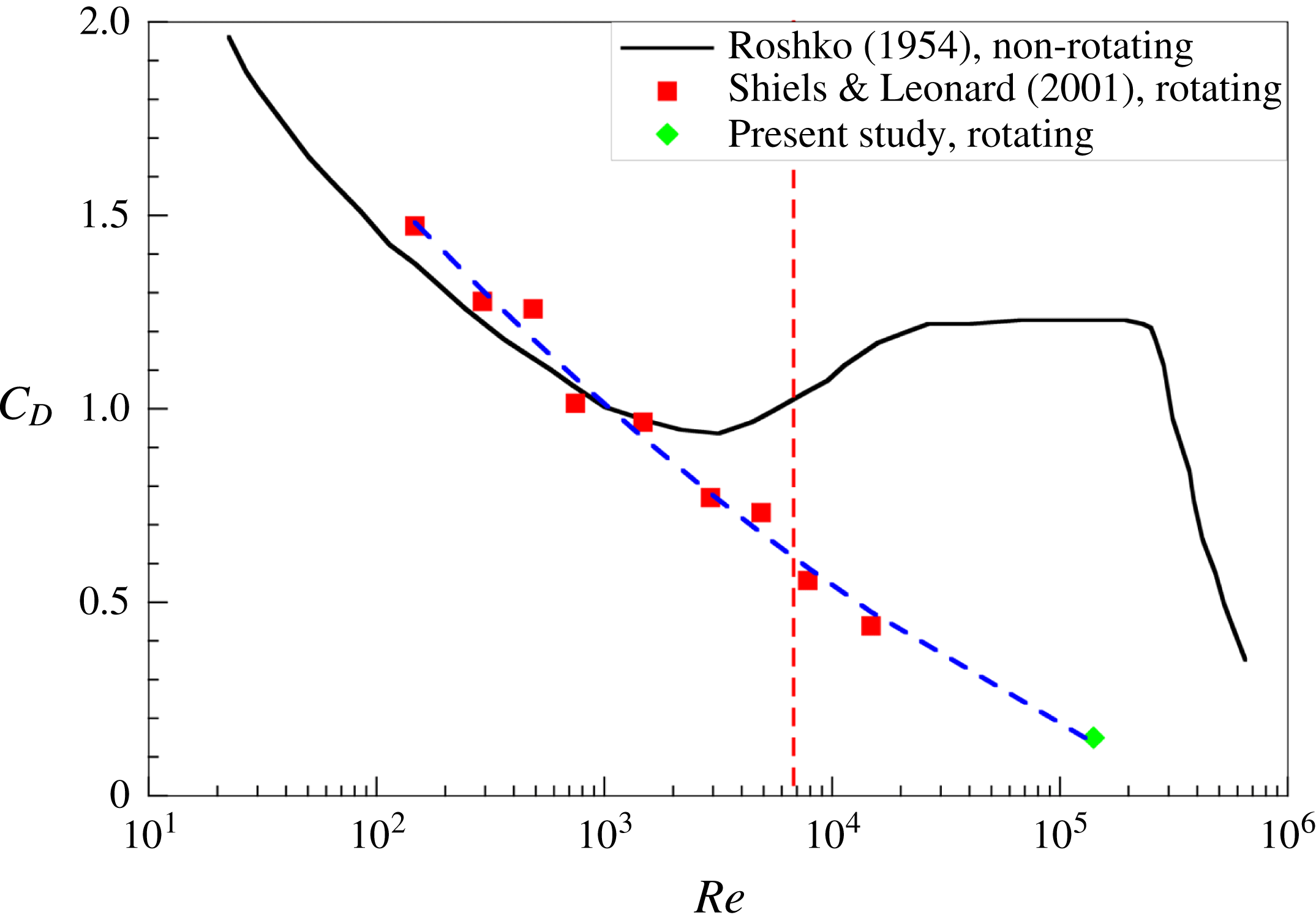
The drag coefficient as a function of
 $Re$
. Black line corresponds to the experimental data obtained by Roshko (Reference Roshko1954) for the non-rotating case. Red squares denote the results by Shiels & Leonard (Reference Shiels and Leonard2001) for
 $\unicode[STIX]{x1D6FA}=2$
and
 $f_{e}=1$
(
 $f\approx 5$
) while green diamond shows the present result for
 $\unicode[STIX]{x1D6FA}=2$
and
 $f=5$
. Blue dashed line serves as a fitting curve expressed by (4.1). Vertical red dashed line shows the critical value
 $Re^{\ast }\approx 6760$
when the control method becomes efficient based on the calculations described in the next section.

To close this section we discuss the effect of
 $Re$
on drag reduction. A compilation of the present results for
 $\unicode[STIX]{x1D6FA}=2$
and
 $f=5$
, the data from Shiels & Leonard (Reference Shiels and Leonard2001) for
 $\unicode[STIX]{x1D6FA}=2$
and
 $f_{e}=1$
(
 $f\approx 5$
) and non-rotating experiments by Roshko (Reference Roshko1954) is shown in figure 24. Indeed, as the Reynolds number increases, the forcing becomes more efficient. At fixed amplitude and high forcing frequency we can approximate
 $C_{D}(Re)$
using the following function:
 $$\begin{eqnarray}C_{D}(Re)=3.047-0.836\log Re+0.053\log ^{2}Re.\end{eqnarray}$$
One interesting observation is that, according to this expression,
 $C_{D}$
approaches zero at
 $Re\approx 5.2\times 10^{5}$
. At the end of the next section we use
 $C_{D}(Re)$
to estimate
 $Re$
when the method becomes energetically efficient.
5 Efficiency and practical implication of rotary oscillations
Although the rotary oscillations lead to significant drag reduction, the question that arises is if the method has a practical relevance and if it is economically feasible. In other words, can the power saved by the drag reduction exceed the power needed to rotate the cylinder in some realistic scenario. Shiels & Leonard (Reference Shiels and Leonard2001) defined a power saving ratio (PSR) as a ratio of the power saved over the power expended to rotate the cylinder against the skin friction, i.e.
 $$\begin{eqnarray}PSR=\frac{P_{saved}}{P_{exp}}.\end{eqnarray}$$
However, they did not account for the power needed to rotate a cylinder with a non-zero mass. Depending on the material, this contribution can dominate. Here we expand the analysis to account also for the cylinder mass.
The power saved due to drag reduction and power needed to rotate the (massless) cylinder against skin friction are defined as
 $$\begin{eqnarray}\unicode[STIX]{x0394}P_{d}={\textstyle \frac{1}{2}}\unicode[STIX]{x1D70C}U_{\infty }^{3}D\unicode[STIX]{x0394}C_{D},\quad P_{\unicode[STIX]{x1D70F}}={\textstyle \frac{1}{2}}\unicode[STIX]{x1D70C}U_{\infty }^{3}D\unicode[STIX]{x1D6FA}\overline{C_{M}\sin \unicode[STIX]{x1D711}}.\end{eqnarray}$$
The non-dimensional moment coefficient has the following form:
 $$\begin{eqnarray}C_{M}(t)=\frac{1}{Re}\left(\left[\int _{0}^{2\unicode[STIX]{x03C0}}\unicode[STIX]{x1D714}_{z}^{wall}\,\text{d}\unicode[STIX]{x1D703}\right]-8\unicode[STIX]{x03C0}\unicode[STIX]{x1D6FA}\sin \unicode[STIX]{x1D711}\right),\end{eqnarray}$$
where the phase of rotation is
 $\unicode[STIX]{x1D711}=2\unicode[STIX]{x03C0}f_{e}t$
as introduced above. It can be shown that the power needed to rotate a cylinder with a certain mass is
 $$\begin{eqnarray}P_{m}={\textstyle \frac{1}{4}}\unicode[STIX]{x1D70C}_{c}U_{\infty }^{3}D\unicode[STIX]{x03C0}f_{e}\unicode[STIX]{x1D6FA}^{2},\end{eqnarray}$$
where
 $\unicode[STIX]{x1D70C}_{c}$
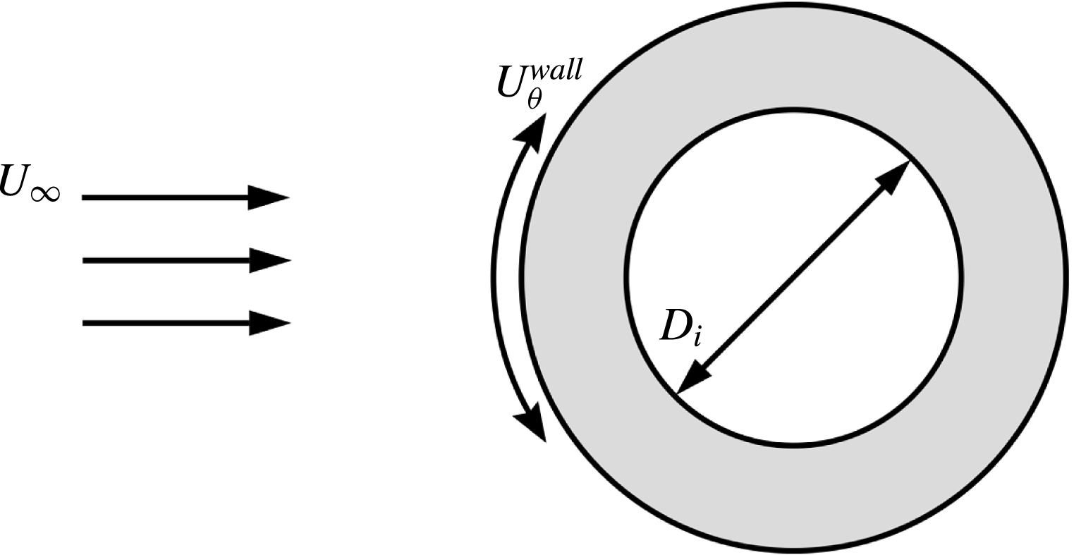
is the density of the cylinder material. Thus, it is obvious that this contribution will dominate over the friction forces, reducing the overall efficiency of the method. One way to overcome this difficulty is to use a hollow cylinder, as shown in figure 25. In that case the rotational power obtains the form
 $$\begin{eqnarray}P_{m}={\textstyle \frac{1}{4}}\unicode[STIX]{x1D70C}_{c}U_{\infty }^{3}D\unicode[STIX]{x03C0}f_{e}\unicode[STIX]{x1D6FA}^{2}(1-r)^{2}(1+r^{2}),\end{eqnarray}$$
where
 $r$
is the ratio of the inner and outer diameter, i.e.
 $D_{i}/D$
. Further we consider a realistic wall thickness of
 $r=0.9$
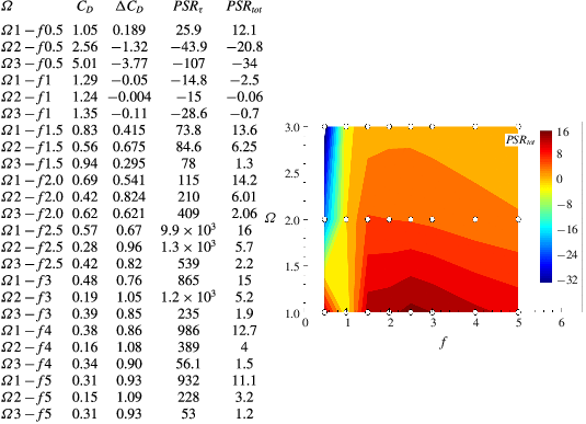
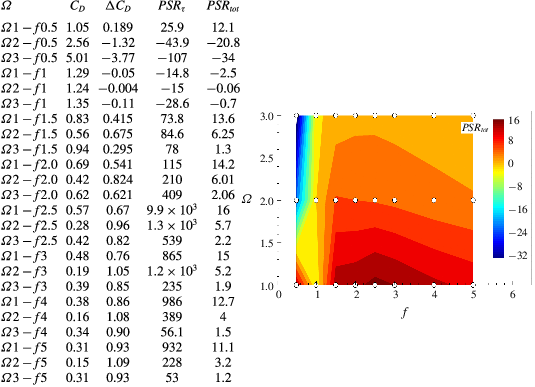
made of aluminium to optimize the power spent on the cylinder rotation. Table 6 shows the main characteristics concerning drag reduction for water flow over a hollow cylinder made of aluminium. Apart from
 $C_{D}$
and
 $\unicode[STIX]{x0394}C_{D}$
compared to the non-rotating case, we analyse
 $PSR_{\unicode[STIX]{x1D70F}}$
following Shiels & Leonard (Reference Shiels and Leonard2001) who used
 $P_{exp}=P_{\unicode[STIX]{x1D70F}}$
meaning that only the friction force is accounted for in the expended power. More relevant is to compute
 $PSR_{tot}$
where
 $P_{exp}=P_{\unicode[STIX]{x1D70F}}+P_{m}$
which is also shown in the table. Note that, due to high
 $Re$
, the friction force is low, thus,
 $P_{\unicode[STIX]{x1D70F}}\ll P_{m}$
. From a practical point of view
 $PSR_{\unicode[STIX]{x1D70F}}$
appears to be irrelevant. Note that
 $P_{m}$
varies linearly with
 $f$
and quadratically with
 $\unicode[STIX]{x1D6FA}$
. This implies that the drag reduction with high frequency is more efficient than the drag reduction with high amplitude. Table 6 confirms this, showing that the highest
 $PSR_{tot}$
(
 $=11.1{-}16$
) is obtained for
 $\unicode[STIX]{x1D6FA}=1$
and various, especially high, frequencies (see the figure accompanying table 6). Admittedly,
 $\unicode[STIX]{x1D6FA}2-f2.5$
and
 $\unicode[STIX]{x1D6FA}2-f3$
also show good results with
 $PSR_{tot}=5.7$
and
 $5.2$
, respectively. This clearly demonstrates the practical potential of the drag reduction mechanism by rotary oscillation of the cylinder.
Schematic picture of flow around a rotating hollow cylinder.

Drag reduction for the water flow over a aluminium hollow cylinder with
 $r=0.9$
. The plot on the right summarizes the results for
 $PSR_{tot}$
in a
 $f-\unicode[STIX]{x1D6FA}$
diagram. White points show the simulated cases.
Another issue is the threshold value of
 $Re^{\ast }$
at which the method becomes energetically efficient. We can use the fitting curve for
 $C_{D}(Re)$
defined by (4.1) and data from the literature, figure 24, to estimate this value in terms of
 $\unicode[STIX]{x0394}C_{D}(Re)$
. The efficiency criterion follows from the
 $\unicode[STIX]{x0394}P_{d}=P_{m}$
condition. Thus, for the
 $\unicode[STIX]{x1D6FA}2-f5$
case and data from Shiels & Leonard (Reference Shiels and Leonard2001) the oscillating aluminium hollow cylinder with
 $r=0.9$
becomes efficient at
 $Re^{\ast }\approx 6760$
. However, we can speculate that attractive energy benefits come at
 $Re>10^{4}$
and lower frequencies of rotation (
 $f\approx 2.5$
).
6 Conclusion
We performed three-dimensional unsteady simulations of flow over a rotary-oscillating infinite cylinder for a set of non-dimensional frequencies
 $f=0.5$
,
 $1$
,
 $1.5$
,
 $2$
,
 $2.5$
,
 $3$
,
 $4$
,
 $5$
and amplitudes
 $\unicode[STIX]{x1D6FA}=1$
,
 $2$
,
 $3$
at a high subcritical Reynolds number,
 $Re=1.4\times 10^{5}$
, and analysed the effects of cylinder oscillations on the flow modification and drag reduction. The study confirms the significant drag reduction for the frequencies larger than
 $1$
, which for
 $f=2.5$
,
 $\unicode[STIX]{x1D6FA}=2$
reached 78 % and even 88 % for
 $f=5$
,
 $\unicode[STIX]{x1D6FA}=2$
. These finding are qualitatively in accord with those of Du & Dalton (Reference Du and Dalton2013) and Tokumaru & Dimotakis (Reference Tokumaru and Dimotakis1991) who also reported a significant drag reduction with a maximum effect of 55 %, but for an order of magnitude lower
 $Re$
number,
 $Re=1.5\times 10^{4}$
. The analysis confirms the expectation that the rotary oscillation control reduces the drag with an increasing efficiency with an increase of the
 $Re$
number. The main findings are summarized as follows:
(i) For
$f\leqslant 1$
, there is no positive effect in the drag coefficient decrease for almost all tested amplitudes. The amplitude in
$C_{D}$
oscillation increases as the size and strength of the main vortex grows due to the imposed rotation. The increase of the mean pressure at the rear part of the cylinder is compensated by a decrease of the mean pressure at the location of the main vortex which results in a mean drag coefficient that is not much different from the non-rotating case.(ii) The increase of the rotational frequency to
$2.5$
leads to a significant reduction in the drag coefficient for all tested amplitudes. The highest drag reduction of 78 % occurs for
$\unicode[STIX]{x1D6FA}=2$
. An additional increase of
$f$
results in a further decrease in the drag coefficient, though at a slower pace, with the highest drop of 88 % obtained for the same amplitude
$\unicode[STIX]{x1D6FA}=2$
, but for a double high frequency,
$f=5$
.(iii) The drag reduction is attributed to the redistribution of the pressure field behind the cylinder, which is caused by dramatic changes in the vortex dynamics associated with the rotation-induced formation of an oscillating boundary layer around the rear cylinder surface.
(iv) The rotary-oscillating cylinder with
$f$
larger than
$1$
produces smaller-scale vortices in the boundary layer that are efficiently removed away from the wall. This leads to shrinking of the low-pressure region in the rear of the cylinder which results in reduction of the drag coefficient.(v) The detachment of the main vortex from the cylinder wall is controlled by the rotational frequency since the vortex is detached from the cylinder by a rotation-generated buffer layer with an opposite-sign vorticity layer placed between the wall and the main vortex. The rotational amplitude determines the strength and thickness of the vorticity layer that grows around the cylinder wall with an increase in the speed of the rotary oscillations. This layer is responsible for stabilization of the stable side but at the same time it also dictates the size of the main vortex that is generated out of the wall-attached separation bubble that grows as a result of cylinder rotation.
(vi) Analysis of a realistic scenario that accounts for the power needed to rotate a cylinder with non-zero mass proves that rotary oscillations of the cylinder is a feasible way to reduce drag. The power saving ratio (
$PSR$
) is
$5.7$
for
$\unicode[STIX]{x1D6FA}=2$
,
$f=2.5$
resulting from a decrease of the drag coefficient by
$78\,\%$
and it goes as high as
$16$
for
$\unicode[STIX]{x1D6FA}=1$
,
$f=2.5$
with a drag reduction of
$56\,\%$
. The drag reduction wat high frequency is more efficient with high amplitude as the rotational power varies linearly with
$f$
and quadratically with
$\unicode[STIX]{x1D6FA}$
.(vii) Using the present results for
$\unicode[STIX]{x1D6FA}2-f5$
and data from Shiels & Leonard (Reference Shiels and Leonard2001) we derived an expression for
$C_{D}(Re)$
, which fits the data in a wide subcritical range of Reynolds numbers. As an example, for a realistic case of a hollow aluminium cylinder with
$r=0.9$
, the drag reduction
$\unicode[STIX]{x0394}C_{D}(Re)$
evaluated from data of Roshko (Reference Roshko1954) gives a threshold value of
$Re^{\ast }\approx 6760$
when the method becomes energetically efficient. We argue that for lower frequencies of rotation (
$f\approx 2.5$
) a solid energy benefit comes at
$Re>10^{4}$
.


Acknowledgements
This work is funded by the Russian Science Foundation grant no. 14-19-01685. The computational resources are provided by Novosibirsk State University Computing Centre (Novosibirsk), Siberian Supercomputer Centre SB RAS (Novosibirsk) and Joint Supercomputer Centre RAS (Moscow).