Introduction
Deep structural foundations (piles) are applied in positions in which the underneath layers of the soil are not capable of bearing the applied structural loads only by foundations. The main reason for applying deep foundation is to transmit the structural applied loads into the stiff denser soil layers in order that they have features to carry structural loads. Therefore, stability and safety of superstructures located on shallow foundations will depend on the pile's behavior. In order to guarantee the stability analysis of shallow foundations, it is very important to attain an exact approximation of axial pile capacity in the soil, especially for design purposes. This problem has become one of the challenging issues in geotechnical engineering since unseen influence parameters and uncertainties affect soil and pile interaction, for instance, the complex behavior of the pile within soil environments, soil disturbing caused by the pile setup and sampling methods, and the load transferring mechanism in the pile (Kiefa, Reference Kiefa1998).
Based on the load transferring characteristics to the underneath layer, the total axial ultimate pile capacity (Q u) generally determines the sum of the pile tip load bearing capacity (Q t) (i.e., dense layers/stiff layers bearing capacity through which applied loads are transmitted onto), and bearing capacity of shaft (Q s) (i.e., bearing capacity transferred through surrounding the friction soil over pile shaft axis) (Niazi and Mayne, Reference Niazi and Mayne2013), which is stated by
 $$Q_{\rm u} = Q_{\rm t} + Q_{\rm s} = q_{\rm t}\cdot A_{\rm t} + \sum\limits_{i = 1}^n {\,f_{{\rm s}(i)}\cdot A_{{\rm s}i}}, $$
where q t is the tip bearing capacity, A t is the pile toe cross-section area, f s is the unit resistance of the shaft within the ith layer of the soil profile in which the pile shaft length is embedded; A si is the contact area that provides shaft frictional resistance with the surrounding soil in the ith layer. The most common methods employed to calculate ultimate axial pile capacity could be categorized into subsequent groups: (1) pile loading tests (PLT), (2) semi-empirical and analytical approaches, and (3) CPT- and SPT-based methods associated with in situ field tests.
Carrying out the PLT method is often time-consuming and expensive in most cases; these tests require advanced equipment with a professional specialist. In addition, most analytical methods often use a number of simplifying assumptions to calculate the load bearing capacity, which encounters many errors. Consequently, some correlations have been proposed by previous researchers to establish a relation between ultimate pile bearing capacity (UPBC) and in situ tests results (Niazi and Mayne, Reference Niazi and Mayne2013). Among some in situ experiments, the cone penetration test (CPT) is considered as the most effective method for describing the soil properties at various depths. In addition, CPT is a commonly used soil exploration survey in engineering applications because it is quick, economic, and could continuously obtain physical soil parameters (Eslami, Reference Eslami1997; Abu-Farsakh and Titi, Reference Abu-Farsakh and Titi2004). In recent years, some researchers developed concepts of advanced artificial intelligence (AI) in different engineering applications, such as engineering mechanics, design of energy-saving buildings, automation, and construction (Coello and Aguirre, Reference Coello and Aguirre2002; Nariman-Zadeh et al., Reference Nariman-Zadeh, Darvizeh and Dadfarmai2003; Hanna, Reference Hanna2007; Padmini et al., Reference Padmini, Ilamparuthi and Sudheer2008; Rossi and Lanzetta, Reference Rossi and Lanzetta2013; Hu et al., Reference Hu, Wang, Wang, Wang and Zhang2014; Zeng et al., Reference Zeng, Tan, Dong and Yang2014; Kontovourkis et al., Reference Kontovourkis, Phocas and Lamprou2015; Salido et al., Reference Salido, Escamilla, Barber, Giret, Tang and Dai2015; Adeniran and El-Ferik, Reference Adeniran and El-Ferik2017; Persson and Ölvander, Reference Persson and Ölvander2017; Thimmisetty et al., Reference Thimmisetty, Tsilifis and Ghanem2017; Al-Refaie et al., Reference Al-Refaie, Judeh and Li2018; Keles, Reference Keles2018; Lin and Huang, Reference Lin and Huang2018; Mirabi and Seddighi, Reference Mirabi and Seddighi2018; Zimmermann et al., Reference Zimmermann, Chen and Shea2018). In recent years, applications of AI models have become widespread through civil engineering projects (e.g., Armaghani et al., Reference Armaghani, Raja, Faizi and Rashid2017, Reference Armaghani, Faradonbeh, Rezaei, Rashid and Amnieh2018; Koopialipoor et al., Reference Koopialipoor, Nikouei, Marto, Fahimifar, Jahed Armaghani and Mohamad2018). In this way, a large number of experts in the field of geotechnical engineering (Shahin, Reference Shahin2010) have made rigorous efforts to employ various AI approaches to establish general traditional equation-based evolutionary computing so as to obtain a more accurate prediction bearing capacity of piles rather than conventional models based on CPT databases (Momeni et al., Reference Momeni, Nazir, Jahed Armaghani and Maizir2014, Reference Momeni, Nazir, Armaghani and Maizir2015, Reference Momeni, Armaghani, Fatemi and Nazir2018). In the case of pile bearing capacity prediction, several research works were conducted to predict pile bearing capacity by using quite a few data-driven models, such as hybrid artificial neural networks (ANN-PSO, ANN-GA and ANN-ICA), support vector machine (SVM), and gene-expression programming (GEP) (e.g., Abu-Kiefa, Reference Abu-Kiefa1998; Alkroosh and Nikraz, Reference Alkroosh and Nikraz2011, Reference Alkroosh and Nikraz2012; Momeni et al., Reference Momeni, Nazir, Jahed Armaghani and Maizir2014; Faizi et al., Reference Faizi, Armaghani, Sohaei, Rashid and Nazir2015; Ebrahimian and Movahed, Reference Ebrahimian and Movahed2016; Moayedi and Armaghani Reference Moayedi and Armaghani2018). Among these AI models, previous investigations have proved that the GMDH network is comparatively more flexible than other AI techniques, such as ANNs and ANFIS (e.g., Najafzadeh et al., Reference Najafzadeh, Barani and Azamathulla2013a, Reference Najafzadeh, Barani and Hessami-Kermani2013b, Reference Najafzadeh, Saberi-Movahed and Sarkamaryan2018; Shaghaghi et al., Reference Shaghaghi, Bonakdari, Gholami, Ebtehaj and Zeinolabedini2017; Harandizadeh et al., Reference Harandizadeh, Toufigh and Toufigh2018). More importantly, there are a few applications of GMDH networks into geotechnical engineering which indicated this model can be employed successfully in some investigations such as mechanical properties of soils (Kalantary et al., Reference Kalantary, Ardalan and Nariman-Zadeh2009)), assessment of tunnel boring machine (Koopialipoor et al., Reference Koopialipoor, Nikouei, Marto, Fahimifar, Jahed Armaghani and Mohamad2018), prediction of soil shear strength in the drained conditions (Mola-Abasi and Eslami, Reference Mola-Abasi and Eslami2018), and evaluation of elasticity modulus of clayed deposits (Naeinia et al., Reference Naeinia, Ziaie Moayeda, Kordnaeija and Mola-Abasib2018). Recently, Harandizadeh et al. (Reference Harandizadeh, Toufigh and Toufigh2018) have employed an improved ANFIS-GMDH model, as a feed-forward network, to obtain an accurate prediction of UPBC. Through their research work, they have developed and combined structure of the ANFIS algorithm with the GMDH algorithm in order to enhance the accuracy level of the ANFIS model; moreover, they optimized the general structure of the ANFIS-GMDH using the gravitational search algorithm (GSA). Hence, this is the second attempt to estimate UPBC by the GMDH. There is no disguising the fact that the application of the GMDH network in the estimation of UPBC has not been fully understood yet. This research subject needs still further efforts to evaluate performance of various hybrid GMDH models. In this way, the crucial aim of this research is to investigate the axial pile bearing capacity prediction using an improved GMDH model by the ANFIS technique whose general structure is optimized by means of particle swarm optimization (PSO). Furthermore, the result of the ANFIS-GMDH model is compared with those yielded by empirical equation CPT-based models.
Basic concepts of CPT-based methods
Schmertmann CPT method
In recent decades, various direct and indirect in situ CPTs were established for subsurface exploration and estimating soil strength parameters  $(\phi \ {\rm {and}} \ c)$ as well as pile capacity prediction; the Schmertmann method was developed based on 108 experimental pile load test (PLTs) results performed on different ranges of piles by Nottingham (Schmertmann, Reference Schmertmann1978) in order to calculate ultimate piles bearing capacity; based on this method, the ultimate pile tip resistance capacity Q P was derived by
 $$Q_{\rm p} = \left( {\displaystyle{{q_{\rm c1} + q_{\rm c2}} \over 2}} \right)\cdot A_{{\rm tip}},$$
where A tip is the pile tip cross-section, q c1 and q c2 indicate the –average pile tip resistance in the range of 0.74D beneath the pile toe region, and in the range of 8D above the pile toe region, respectively (Schmertmann, Reference Schmertmann1978). The average resistance of the cone tip is derived from the representation of the failure surface presumed to trace the logarithmic shape as presented by Begemann (Reference Begemann1963). This method bounds q c1 and q c2 values to 15 MPa. According to the Schmertmann ethod (Schmertmann, Reference Schmertmann1978), the skin friction resistance is expressed by Eqs (3) and (4), respectively, for clayey and sandy soils:
 $$Q_{\rm s} = \alpha _{\rm c}\,f_{\rm s}\,A_{\rm s}\quad {\rm in}\,{\rm clay},$$
 $$Q_{\rm s} = \alpha _{\rm s}\left[ {\sum\limits_{d = 0}^{8D} {\displaystyle{1 \over 2}f_{\rm s}A_{\rm s}} + \sum\limits_{d = 8D}^L {\,f_sA_{\rm s}}} \right]\quad {\rm in}\,{\rm sand},$$
where D and A s denote the equivalent pile diameter or pile width and soil–pile contact area, respectively; α c and α s denote resistance of the shaft to the sleeve friction ratio for clayey and sandy soils; α c values vary from range of 0.2 to 1.2 and is a function of sleeve friction values while α s values depend on pile embedded length to equivalent diameter of pile ratio varying from 0.4 to 4 values. f s denotes the average friction of the shaft sleeve.
De Kuiter and Beringen CPT method
After Schmertmann, another effective CPT predictive method was extended by De Kuiter and Bringen (Reference De Kuiter and Beringen1979) based on experimental results carried in some regions of the North ocean. They indicated that in clayey soil, the unit pile toe resistance and shaft resistance capacity were identified from the undrained soil shear strength based on Eqs (5) and (6), respectively.
 $${\rm The}\,{\rm unit}\,{\rm pile}\,{\rm tip}\,{\rm resistance}\,{\rm in}\,{\rm clay}\,{\rm soils}:q_{\rm p} = N_{\rm c}\,S_{\rm u},$$
 $${\rm The}\,{\rm unit}\,{\rm shaft}\,{\rm resistance}\,{\rm in}\,{\rm clay}\,{\rm soils}:f = {\alpha} ^{\prime}\,S{}_{\rm u},$$
where α′ denoting the cohesion factor is taken in (OC) clay to be equal to 0.5, and for (NC) clay equal to 1; N c denotes the bearing capacity coefficient and S u demonstrates the undrained shear strength which is derived from
 $$S_{\rm u} = \displaystyle{{q_{{\rm ca}}} \over {N_k}},$$
in which N k– denotes the cone coefficient varying within the range of 520; in addition, according to this method, the unit skin frictional resistance in the sand was defined through
 $$f = \min \lcub {\,f_{\rm s}\comma \,q_{\rm c}/300\comma \,120\,{\rm kPa}}, \rcub $$
where q c and f s are the unit resistance of the cone tip and unit sleeve friction, respectively.
Similarly, they observed that the pile toe resistance capacity in the sand was found to be the same as that obtained by the Schmertmann method procedure (Schmertmann, Reference Schmertmann1978).
Bustamante and Gianeselli CPT method (LPC/LPCT)
The proposed LPC method was conducted by Bustamante and Gianeselli (Reference Bustamante and Gianeselli1982) carrying out some experimental tests on piles for developing a French highway project. In this approach, the unit pile toe resistance and unit pile shaft resistance are stimulated from cone tip resistance by ignoring the sleeves friction. The unit resistance of the pile tip is estimated using the following equation:
 $$q_{\rm p} = k_{\rm b}q_{{\rm ca}},$$
in which q ca is the average value of q c over the influence zone ranging from 1.5D (pile diameter) below and above of the pile toe region, and k b is a coefficient dependent on soil properties and the pile setup method. The unit shaft resistance capacity was established using the following equation:
 $$f = \displaystyle{{q_{\rm c}} \over {k_{\rm s}}},$$
in which q c is the mean resistance of the cone tip along the pile length and k s is a coefficient depending on pile materials and setup methods.
Materials
A proposed ANFIS-GMDH-PSO model was developed based on 108 data sets derived from the literature. In the developed model, the cluster parameters and ANFIS membership functions were improved and adjusted by applying the PSO technique. This section discussed data source details and effective input variables presented by the hybrid ANFIS-GMDH-PSO model. A database consists of 108 samples derived from previous research (Eslami, Reference Eslami1997; Nejad et al., Reference Nejad, Jaksa, Kakhi and McCabe2009).
The Dara source covers various variables including static PLT (ML or CRP), pile materials (steel, concrete, composite), pile set-up method (drilled or driven), and pile end type (open or closed); the effective input variables are taken into account as the pile tip cross-section A t, A s is the sleeve shaft cross-section, the average resistance of cone tip value along shaft length  $\bar{q}_{\rm c-{\rm shaft}}$, and the average resistance of the cone tip value over pile tip influence zone
 $\bar{q}_{{\rm c}-{\rm tip}}$.
The measured ultimate bearing capacity P u is derived from full-scale static pile loading test results. For piles that failed during the test, the failure load was considered as the UPBC; for other piles, 80% failure criteria proposed by Hansen was used (Kondner, Reference Kondner1963). The ANFIS-GMDH-PSO model output is the axial pile load bearing capacity (P u) expressed as a function of effective input parameters in general form by
 $$P_{\rm u} = f\,(A_{\rm t}\comma \,A_{\rm s}\comma \,\bar{q}_{{\rm c}-{\rm shaft}}\comma \,\bar{q}_{{\rm c}-{\rm tip}}\comma \,\bar{\,f}_{\rm s}).$$
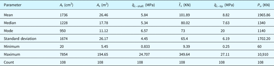
The under-study parameter description used to develop the model is summarized in Table 1.
Statistical variables description used in the developed ANFIS-GMDH-PSO model

Methodology
The research methodology is explained in subsequent sections; first, a brief description of different AI methods was described in detail including ANFIS [Description of adaptive neuro-fuzzy inference system (ANFIS)], GMDH type neural network structures (Description of GMDH type neural network framework), and PSO algorithm (Description of PSO framework); then the hybridization process of the ANFIS-GMDH network structure was explained (Development of hybrid ANFIS-GMDH structure) and finally the developed ANFIS-GMDH model was optimized based on the PSO algorithm over the hybrid ANFIS-GMDH topology structure (Development of hybrid ANFIS-GMDH-PSO algorithm).
Description of ANFIS
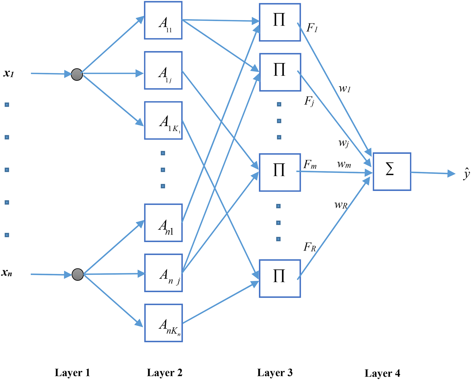
The ANFIS structure used in this study is shown in Figure 3 (Zhang et al. Reference Zhang, Ding, Rao and Bi2006). The rules of the fuzzy inference system applied in the ANFIS network structure are demonstrated based on Takagi–Sugeno–Kang’ approach that utilizes membership functions instead of using fuzzy sets theory applied through the fuzzy inference system of Mamdani's approach (Zadeh, Reference Zadeh1996). For simplicity, a fuzzy inference rule of R r applying the first-order TSK method (Takagi and Sugeno, Reference Takagi and Sugeno1993) could be expressed by
 $$R^{\,r}:\,{\rm If}\,x_1\,{\rm is}\,A_{1j}\,{\rm AND}\, \ldots \,{\rm AND}\,x_n\,is\,A_{nj}\,{\rm then}\,\mathop{y}\limits^{\frown}\,{\rm is}\,w_r$$
in which x i indicates the ith input variable of the neuro-fuzzy system (n represents the input variables number), A ij denotes the jth membership function of antecedent part of the input variable x i (j = 1, 2, …, K i), K i expresses the number of fuzzy sets for each input variable x i, and w r are the consequent part parameters (r = 1, 2, …, R),  $\mathop{y}\limits^{\frown}$ is single output, and
 $R = \prod _{i = 1}^n \,K_i$ is fuzzy rules number (number of rules) made by taking into account all fuzzy sets combination. The ANFIS network consisted of four different layers described briefly below. Layer 1 (Layer of input): Through passing this layer, the x i values are entered into the second layer without any changes.
Layer 2 (Layer of fuzzification): Through the nodes of this layer, the Gaussian-type arbitrary membership functions are defined with σ ij (standard deviation) and c ij (center) for x i (input variable) by
 $$A_{ij}(x_i) = \exp -\displaystyle{{{(x_i-c_{ij})}^2} \over {\sigma _{ij}^2}}\comma \,\,j = 1\comma \, \ldots\comma \, K_i.$$
Layer 3 (Layer of inference): The nodes within this layer generate an antecedent part of the fuzzy rule using fuzzy AND/OR operators to obtain the firing strength of F r extracted from the fuzzy rule of the rth based on membership functions values using the following equation:
 $$F_r = \prod\limits_{i = 1}^n {A_{ij}(x_i} )\comma \,r = 1\comma \,2\comma \,...\comma \,R\,{\rm and}\,j = 1\comma \,2\comma \,...\comma \,K_i$$
Layer 4 (Layer of output): This layer is composed of a single node denoted as the final ANFIS output. The estimated output for the ANFIS is described below in Eq. (15):
 $$\mathop{y}\limits^{\frown} = \sum\limits_{r = 1}^R {F_r} w_r$$
Description of the GMDH type neural network framework
The idea associated with ANNs stimulated through the modeling structure of the complex human brain is known as a non-linear, parallel performing approach (Haykin et al., Reference Haykin, Nie and Currie1999). The GMDH type neural network structure is the self-organizing method by which a behavior system is identified by the assessment of its performances over a provided set of multi-input single output data set (x i, x j) , (i = 1, 2, …, M). The concept of the GMDH network is to make an analytic function within a feed-forward network determined by a polynomial transfer function in which coefficients are attained by applying the particular regression process (Najafzadeh et al., Reference Najafzadeh, Barani and Azamathulla2013). By applying the GMDH algorithm, a model is displayed as a set of neurons through which various sets in every single layer are usually interconnected through a quadratic polynomial, creating new neurons inside the subsequent layer. These types of representation is employed to map input space to output space (Najafzadeh and Azamathulla, Reference Najafzadeh and Azamathulla2013; Najafzadeh et al., Reference Najafzadeh, Barani and Azamathulla2014; Najafzadeh, Reference Najafzadeh2015). The basic description of the identification issue is to uncover a function  $(\hat{f})$ utilized as opposed to the desired function (f) as a way to predict the output result
 $(\hat{y})$ for any provided input vector X = (x 1, x 2, x 3, …, x n) as close as possible toward the target value (y). For that reason, M observations involving multivariable input–single variable output data set are established by Eq. (16) (Najafzadeh and Barani, Reference Najafzadeh and Barani2011; Najafzadeh and Azamathulla, Reference Najafzadeh and Azamathulla2013; Najafzadeh and Lim, Reference Najafzadeh and Lim2015):
 $$y_i = f\lpar {x_{i1}\comma \,x_{i2}\comma \,x_{i3}\comma \, \ldots\comma \,x_{in}} \rpar \,\comma \,\,\lpar {i = 1\comma \,2\comma \,3\comma \, \ldots M} \rpar. $$
It could be practical to train a GMDH type of the artificial neural network to estimate predicted values  $(\hat{y}_i)$ considered to be for each provided input vector (X):
 $$\hat{y}_i = \hat{\,f}(x_{i1}\comma \,\,x_{i2}\comma \,x_{i3}\comma \,...\comma \,x_{in})\,\,\,(i = 1\comma \,2\comma \,3\comma \, \ldots\comma \, M).$$
The main issue is to specify a GMDH type neural network to ensure square of the differences between observed and expected output values minimized as follows:
 $$\sum\limits_{i = 1}^M {\lsqb {\hat{\,f}(x_{i1}\comma \,\,x_{i2}\comma \,\,x_{i3}\comma \, \ldots\comma \,\,x_{in})-y_i} \rsqb } ^2\,\,\Rightarrow \min {\!}.$$
An elaborate discrete type of the Volterra functional series, referred to as Kolmogorov–Gabor polynomial, can present the general relationship among input and output parameters mapping. As a result,
 $$ \eqalign{ y = a_0 + \sum\limits_{i = 1}^n {a_ix_i + \sum\limits_{i = 1}^n {\sum\limits_{\,j = 1}^n {a_{ij}x_ix_j + \sum\limits_{i = 1}^n {\sum\limits_{\,j = 1}^n {\sum\limits_{k = 1}^n {a_{ijk}x_ix_jx_k + \ldots}}}}}}. $$
This specific full form of mathematical description is typically exhibited by using a solution of partial quadratic polynomials made from simply two variables (neurons) by applying
 $$\hat{y} = G(x_i\comma \,x_j) = a_0 + a_1x_i + a_2x_j + a_3x_ix_j + a_4x_i^2 + a_5x_j^2. $$
By using this approach, the description of a partial quadratic is recursively applied to the interconnected neurons network to develop the standard mathematical relation concerning input and output provided in Eq. (19). The a i coefficients in Eq. (20) are computed by applying the regression method to decrease the main difference between observed output values (y) and predicted the output ones  $(\hat{y})$ for each pair of input parameters (x i, x j). Clearly, a tree of polynomials is developed by utilizing the quadratic type provided in Eq. (20) whose coefficients are achieved by the least-square method (Najafzadeh et al., Reference Najafzadeh, Barani and Azamathulla2013; Najafzadeh and Saberi-Movahed, Reference Najafzadeh and Saberi-Movahed2019). The coefficients of each quadratic function Gi are obtained for an optimum fitting for that output associated with the total pairs of input–output data sets based on minimizing Eq. (21) criteria:
 $$E = \displaystyle{{\sum\nolimits_{i = 1}^M {{(y_i-G_i(x_i\comma \,x_j))}^2}} \over M}\,\Rightarrow \,\,\min{\!}. $$
For the standard form of the GMDH-type neural network formula, all possibilities of two independent variables from the total n input variables are taken into account to construct the regression polynomial by using Eq. (20) that most closely fits the dependent observations (y i , i = 1, 2, …, M) based on the least-squares perspective.
Therefore, 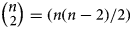 $ \vscale105%\scale120% \big( { {\vskip-5pt n} \cr \scale90%{\hskip-5pt \vskip3.8pt 2} }\scale120%\vscale105%\big ) = (n(n-2)/2)$ neurons are established within the first hidden layer from the feed-forward network using the observations {(y i, x ip, x iq); (i = 1, 2, 3, …, M)} using p, q ∈ {1, 2, 3, …, n} in the form
 $$\left[ {\matrix{ {x_{1p}} & {x_{1q}} & \vdots & {y_1} \cr {x_{2p}} & {x_{2q}} & \vdots & {y_2} \cr \cdots & \cdots & \cdots & \cdots \cr {\vskip-5pt x_{Mp}} & {\vskip-5pt x_{Mq}} & \vdots & {\vskip-5pt y_M} \cr}} \right].$$
From the quadratic sub-expression, using Eq. (20) per each row of M data triples, the below matrix formulation is achieved through Eqs (23)–(26), respectively:
 $$Aa = Y,$$
 $$a = \lcub {a_0\comma \,a_1\comma \,a_2\comma \,a_3\comma \,a_4\comma \,a_5} \rcub, \,$$
 $$Y = \lcub {y_1\comma \,y_2\comma \,y_3\comma \, \ldots\comma \, y_M} \rcub ^T,$$
 $$A = \left[ {\matrix{ 1 & {x_{1p}} & {x_{1q}} & {x_{1p}x_{1q}} & {x_{1p}^2} & {x_{1q}^2} \cr 1 & {x_{2p}} & {x_{2q}} & {x_{2p}x_{2q}} & {x_{2p}^2} & {x_{2q}^2} \cr \cdots & \cdots & \cdots & \cdots & \cdots & \cdots \cr 1 & {x_{Mp}} & {x_{Mq}} & {x_{Mp}x_{Mq}} & {x_{Mp}^2} & {x_{Mq}^2} \cr}} \right].$$
The least-squares technique from the multiple regression analysis leads to a solution of the characteristic equations in the following form:
 $$a = (A^TA)^{-1}\,A^TY.$$
The solution determines the coefficient vector of Eq. (20) for all range of M data set triples. It is observed that this process is repeated for every neuron of any succeeding hidden layer as outlined by the interconnection topology in this network (Najafzadeh and Tafarojnoruz, Reference Najafzadeh and Tafarojnoruz2016; Najafzadeh et al., Reference Najafzadeh, Saberi-Movahed and Sarkamaryan2018; Najafzadeh and Saberi-Movahed, Reference Najafzadeh and Saberi-Movahed2019).
Development of the hybrid ANFIS-GMDH structure
In this part, the new structure of the GMDH type neural network was discussed in which partial descriptions (PDs) are ANFIS networks having two inputs in place of the RBF structure. Each PD is an ANFIS network with two inputs in which the number selection of membership functions per each input is changeable. Accordingly, the output of each PD is defined as given in Eq. (28) and Eq. (29):
 $$F^{{\rm pm}} = \displaystyle{{\sum\nolimits_l^n {\sum\nolimits_k^n {\mu _{A_l}(x_1^{{\rm pm}} )\,\mu _{B_k}(x_2^{{\rm pm}} )}} f_{{\rm lk}}^{{\rm pm}}} \over {\sum\nolimits_l^n {\sum\nolimits_k^n {\mu _{A_l}(x_1^{{\rm pm}} )\,\mu _{B_k}(x_2^{{\rm pm}} )}}}}, $$
 $$f_{{\rm lk}}^{{\rm pm}} = q_{{\rm lk}}^1 x_1 + q_{{\rm lk}}^2 x_2 + q_{{\rm lk}}^3, $$
in which m is PD number in the pth layer, n is the selected number of membership functions intended for inputs, and q coefficients are real numbers. In this case, the network output is achieved based on
 $$y = \displaystyle{1 \over M}\sum\limits_{m = 1}^M {F^{{\rm pm}}}. $$
The notation M refers to the number of PDs in the last layer.
Description of the PSO framework
The PSO technique is one of the metaheuristic algorithms inspired based on animals’ swarm behavior presented by Eberhart and Kennedy (Reference Eberhart and Kennedy1995). The primary idea lies in simulating the social behavior of creatures such as birds and floating fish in a multidimensional space. In the PSO algorithm, the population size consists of a set of random individual particles (M) dispersed in a D-dimensional searching space (Eberhart and Kennedy, Reference Eberhart and Kennedy1995).
Initially, to develop a PSO structure, a random position vector of  $P^m = (P_1^m\comma \,P_2^m\comma \, \ldots\comma \,P_D^m )$ is defined for the data set domain and a vector of random velocity of
 $V^m = (V_1^m\comma \,V_2^m\comma \, \ldots\comma \,V_D^m )$ computed for m = (1, 2, …, M) in the interval of [− V max + V max] for each particle. Each particle follows the two best vectors; one vector denoted as the best particle position as
 ${P\rm bes}{\rm t}^m = ({P\rm best}_1^m\comma \,{P\rm best}_2^m\comma \,...\comma \,{P\rm best}_D^m )$ that each particle experiences so far associated with the minimum cost function value. Another vector is denoted as the particle's best global position of Pbestg = (Pbestg1, Pbestg2, …, PbestgD) associated with the minimum cost function value obtained among the whole population. To find the optimal solution, position and velocity vectors of each particle are updated iteratively through Eqs (31) and (32) for their fly-experience in search space (Poli et al., Reference Poli, Kennedy and Blackwell2007).
 $$V_d^m (t + 1) = W\cdot V_d^m (t) + \phi _1r_1({\rm Pbes}t_d^m (t)-P_d^m (t)) + \phi _2r_2({\rm Pbes}{\rm t}_{{\rm gd}}(t)-P_d^m (t)),$$
 $$P_d^m (t + 1) = P_d^m (t) + V_d^m (t + 1)\,\,\,\,\,{\rm for}\,m = 1\comma \,2\comma \,...\comma \,M\comma \,\,\,\,d = 1\comma \,2\comma \,...\comma \,D,$$
in which W is the factor of inertia governing the effect of the previous velocity on the current velocity; and ϕ 1 and ϕ 2 denote the cognitive and social parameters, respectively, which control the velocity of the particles toward Pbest(m) and Pbestg; r 1 and r 2 are generated random numbers in the interval [0, 1] and t represents the number of iterations (Najafzadeh et al., Reference Najafzadeh, Barani and Hessami-Kermani2015).
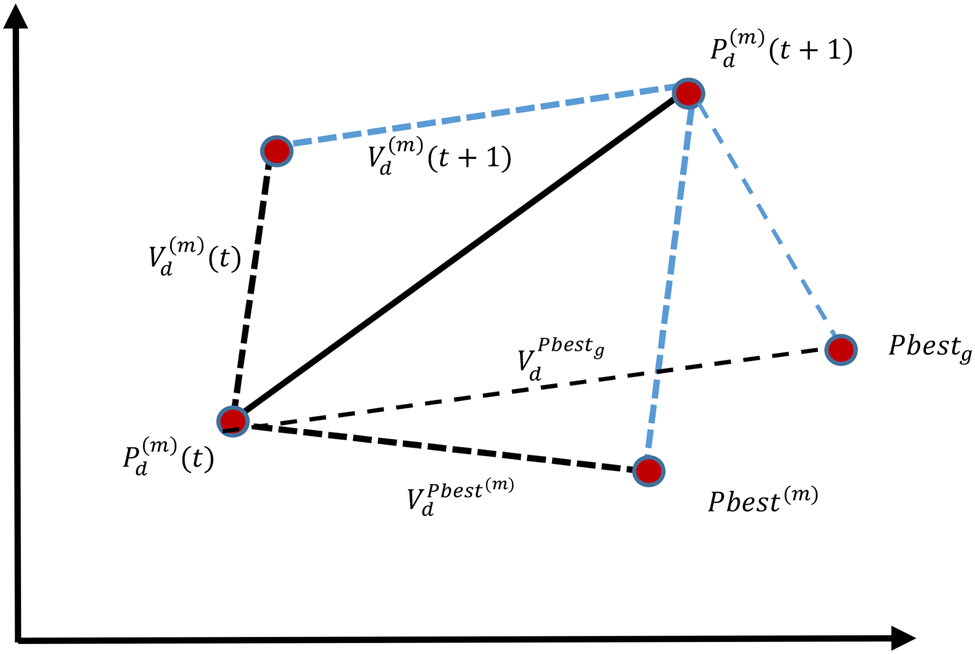
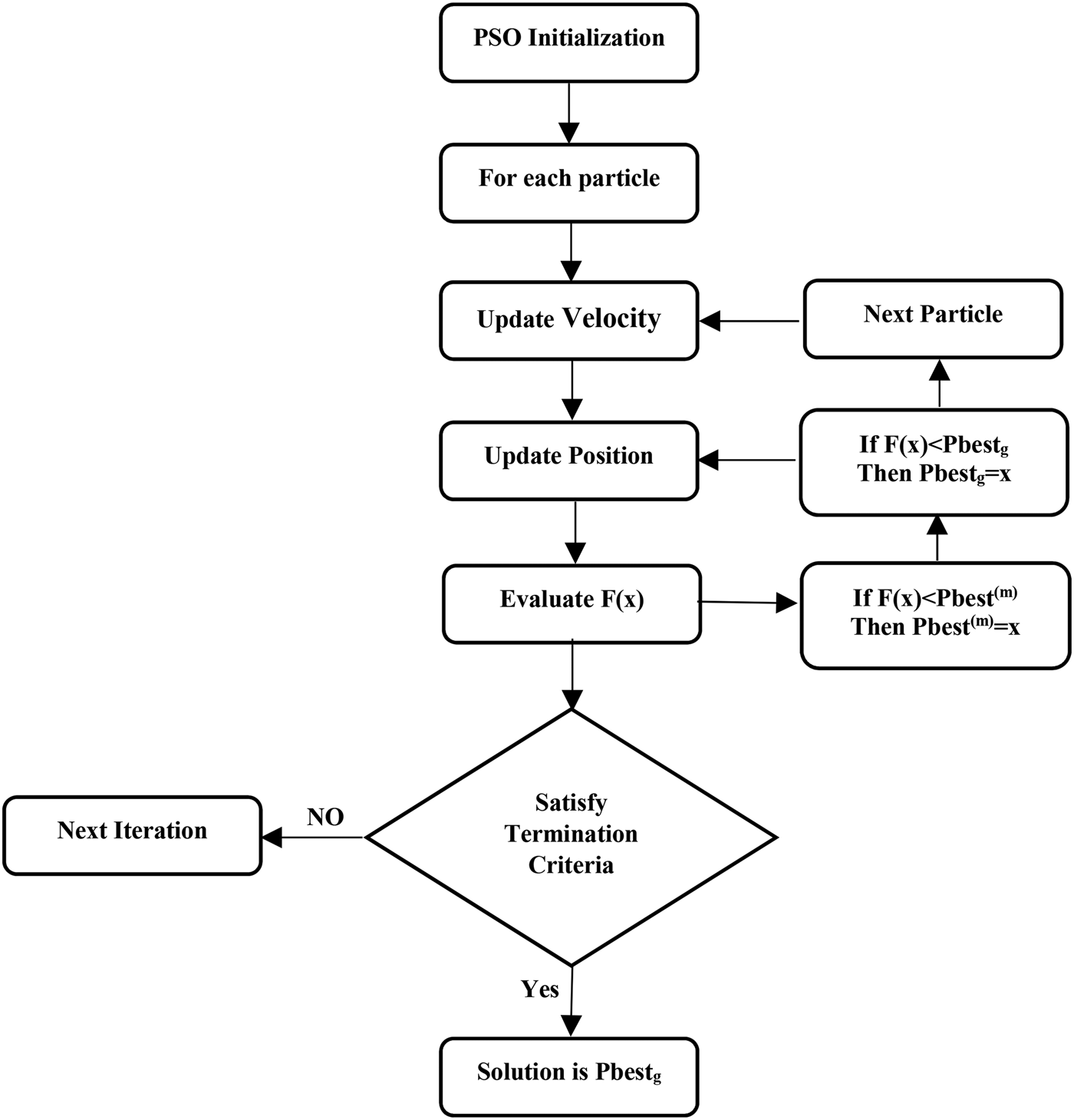
To stop swarm exploration and divergences, the velocity of all particles must be limited at intervals [− V max, V max] in each repetition, where V max relies on the maximum velocity that is allowed for particles. At higher values than V max, particles tend to go beyond the optimal solution, and in opposite cases, the particles are trapped in the local minima. The exploration mechanism of the optimization of particle swarm (PSO) is shown in Figure 1. The flowchart of the PSO algorithm is given in Figure 2.
PSO search mechanism.

Flowchart of the PSO algorithm.

Development of the hybrid ANFIS-GMDH-PSO algorithm
The PSO approach was applied for optimizing the ANFIS-GMDH structure and improving membership function parameters. Under such circumstances, the design of the ANFIS-GMDH involves the selection of fuzzy rules assigned higher firing strength (F r). This selection causes to reduce the ANFIS-GMDH network error and number of selection rules. In the hybrid ANFIS-GMDH-PSO network model, a position vector (P m) and velocity vector (V m) were assigned for each particle in the following form:
 $$\eqalign{P^m = (e_1^m\comma \,e_2^m\comma \, \ldots \,e_R^m\comma \,c_{11}^m\comma \, \ldots\comma \,c_{1K_1}^m\comma \, \ldots \,c_{nK_n}^m\comma \, \sigma _{11}^m\comma \, \ldots\comma \cr \sigma _{1K_1}^m\comma \, \ldots\comma \,\sigma _{nK_n}^m\comma \,w_1^m\comma \, \ldots\comma \,w_R^m ),}$$
 $$V^m = (V_1^m\comma \,V_2^m\comma \, \ldots\comma \,V_R^m\comma \,V_{R + 1}^m\comma \, \ldots\comma \,V_z^m ).$$
The  $(e_1^m\comma \,e_2^m\comma \, \ldots\comma \,e_R^m )$ vector demonstrates the fuzzy rules effectiveness rate. Each
 $e_r^m$ for (r = 1, 2, …, R) references to the connecting link between layer 3 and layer 4. In case the value of
 $e_r^m$ is equal to one, it indicates that the relevant fuzzy inference rule is enabled, in other cases the fuzzy rule effect is ignored. It is noted that a fuzzy rule is preserved in terms of
 $\tilde{p}_r \gt \xi$ criteria (Fig. 3).
ANFIS network structure.

In which ξ denotes the amount of threshold specified by choice $({\rm i}{\rm. e}.\comma \,\,\xi = 5\% )$ and
 $\tilde{p}_r$ is the pattern concentration percentage calculated as
 $\tilde{p}_r = (p_r/Q) \times 100(\% )$; in this relation, p r indicates the number of patterns available in R r with a firing strength of F r >0.5, and Q point outs to the number of training samples (Elloumi et al., Reference Elloumi, Krid and Masmoudi2015).
The optimization problem was defined based on,
 $${\rm Minimize}\,{\rm fitness}\,(P^m) = \alpha \cdot F_1(P^m) + \beta \cdot \displaystyle{1 \over {F_2(P^m)}}.$$
The overall ANFIS network structure was described by a vector of  $(e_1^m\comma \,e_2^m\comma \, \ldots\comma \,e_R^m )$. Therefore, the functions of F 1 and F 2 introduced through Eqs (36) and (37), respectively, are applied to P m,
 $$F_1(P^m) = 1 + \sum\limits_{r = 1}^R {e_r^m}, $$
 $$F_2(P^m) = \frac{1}{(1/2)\cdot \sum\nolimits_{q = 1}^Q ({\mathop{y}\limits^{\frown}}_q^m -y_q)^2} $$
where  $\mathop{y}\limits^{\frown}_q$ and y q represent the adaptive neuro-fuzzy system output and observed target of the qth training sample.
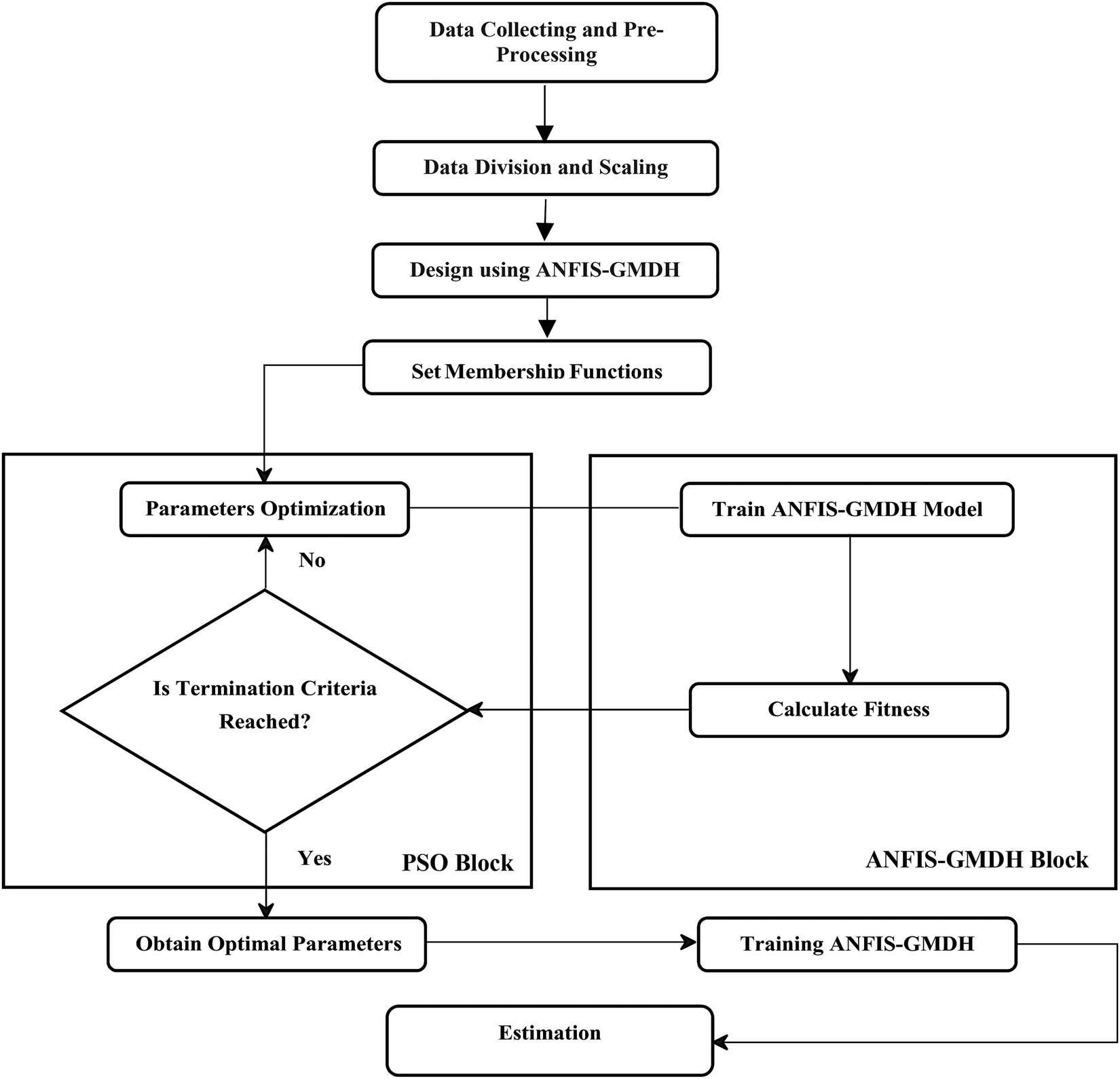
The workflow of the developed ANFIS-GMDH-PSO flowchart is shown in Figure 4.
Flowchart of the ANFIS-GMDH model optimized by the PSO algorithm.

Results and discussion
Hybrid ANFIS-GMDH-PSO model performance
Although several models can be derived from the hybrid ANFIS-GMDH-PSO model, the best fitted model must meet some statistical criteria prior to final model selection. From this perspective, a number of previously available statistical indices criterion have been presented by some researchers.
The precision level of these models was assessed by various statistical parameters. In this study, the coefficient of regression (R), root mean square error (RMSE), and mean absolute error (MAE) are
 $$R=\frac{\sum_{i=1}^n(h_i-{\bar{h}})(t_i-\bar{t})}{\sqrt{\sum_{i=1}^n(h_i-{\bar{h}})^2\sum_{i=1}^n(t_i-\bar{t})^2}}, $$
 $${\rm RMSE} = \sqrt {\displaystyle{{\sum\nolimits_{i = 1}^n {{(h_i-t_i)}^2}} \over n}}, $$
 $${\rm MAE} = \displaystyle{1 \over n}\sum\limits_{i = 1}^n {\vert {h_i-t_i} \vert }. $$
In the above-mentioned equations, h and t are the predicted P u and observed P u values, respectively.  $\bar{h}$ and
 $\bar{t}$ represent the average value of predicted P u and average P u values obtained from measured pile loading test results (target values), respectively. These statistical criteria were frequently used to assess performance of various hybrid GMDH models in the field of the scouring process at hydraulic structures (e.g., Najafzadeh et al., Reference Najafzadeh, Barani and Azamathulla2013, Reference Najafzadeh, Barani and Hessami-Kermani2015). From Eqs (38)–(40), it was observed that there are relatively good correlations between measured values (Observed Targets) and predicted values (model output) in cases where R > 0.8 or R 2 > 0.64, which indicates the perdition capability by proposed model.
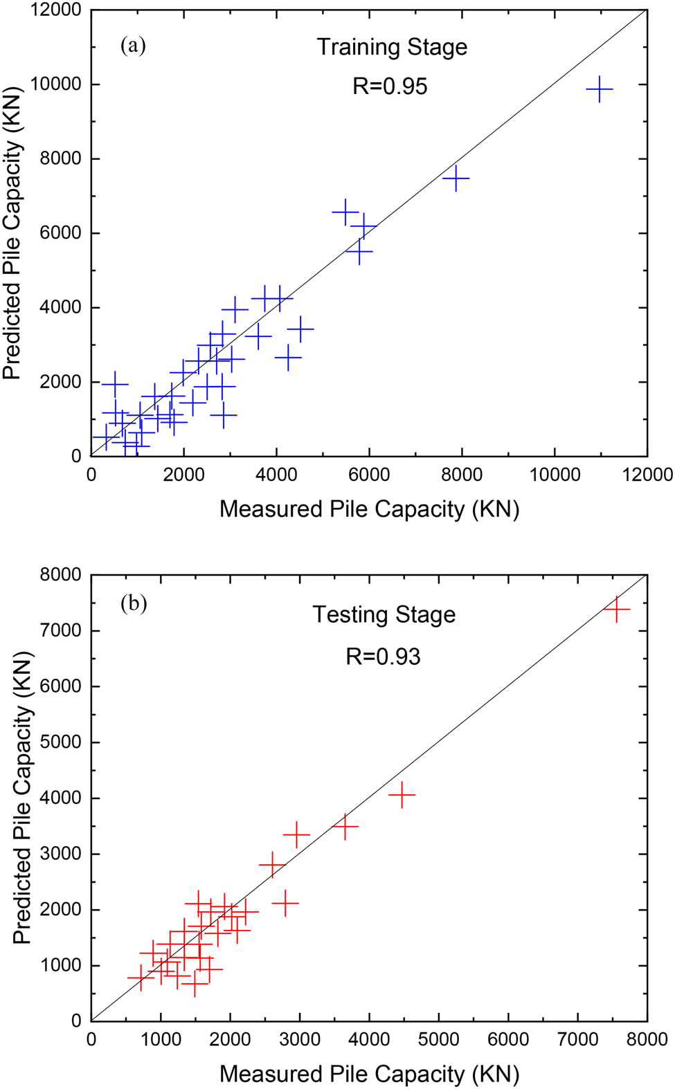
It is noted that the sole use of R as the overall performance model's assessment is not normally sufficient to determine model precision since it is sensitive to the increase and relative variance between measured values and predicted values. Therefore, RMSE and MAE were also selected as auxiliary criteria in order to assess the accuracy level of the AI model. The best performance of AI is at the mercy of being zero in RMSE and MAE values. To display the ability of the ANFIS-GMDH-PSO model in pile bearing capacity prediction, the regression plot of measured values versus the predicted values is shown in Figure 5a,b for both training and testing stages.
Statistical and regression plot of the ANFIS-GMDH-PSO model in (a) training stage and (b) testing stage.

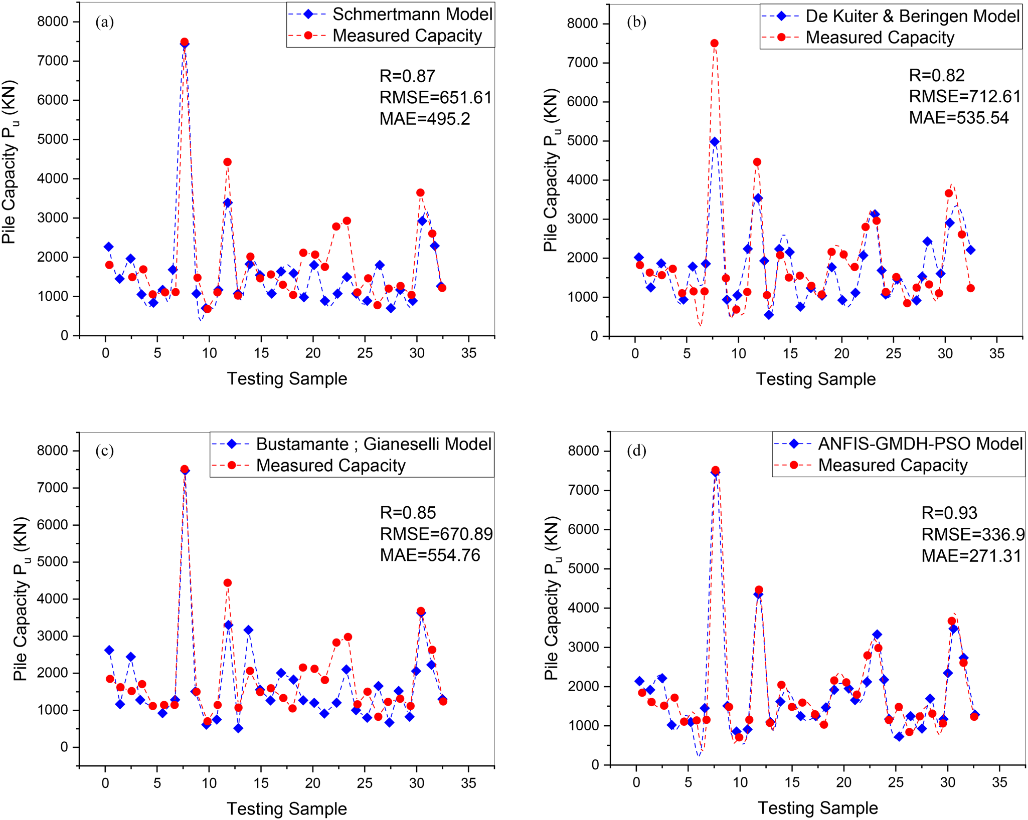
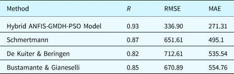
From Table 2, it was found that the ANFIS-GMDH model has gained the highest R value and the lowest values of RMSE and MAE, estimating P u in comparison with empirical equations. In addition, relatively close values of R, RMSE, and MAE in the training and testing data set showed that this AI model benefits from highly convincing performance. In order to ensure ANFIS-GMDH-PSO model performance, its predictability should be evaluated compared to empirical methods. In this regard, the same testing data set applied to the hybrid ANFIS-GMDH-PSO model was considered for comparing in various CPT-based methods. The results of the comparative analysis among different models are shown in Figure 6. The values obtained from CPT-based methods are based on previous studies (Eslami, Reference Eslami1997; Kordjazi et al., Reference Kordjazi, Nejad and Jaksa2014).
Comparison of measured vs predicted values (P u) by various methods for the testing data set.

Statistical analysis results in various applied methods for the test data set

The statistical parameters obtained from the developed network model (ANFIS-GMDH-PSO) are compared with those obtained by various empirical CPT-based models: Schmertmann (Reference Schmertmann1978), De Kuiter and Beringen (Reference De Kuiter and Beringen1979), and Bustamante and Gianeselli (Reference Bustamante and Gianeselli1982). Statistical results are presented in Table 2. To evaluate results obtained from the ANFIS-GMDH-PSO model and conventional methods, graphical results of empirical equations are shown in Figure 6 for calculating the UPBC.
Sensitivity analysis
Sensitivity analysis simulation was performed in this research to evaluate the prediction and validation ability of the developed ANFIS-GMDH-PSO model with the aid of statistical indices criterion in addition to comparing the results presented by some researchers through CPT-based models in this field.
Although the ANFIS-GMDH-PSO model showed that the developed model has a good enough approximation capability, it is necessary to consider the physical behavior of the model from an engineering perspective point view. For this purpose, the behavior and response of the model could be assessed based on individual various input variables and must compare with available empirical or theoretical approaches presented in previous studies.
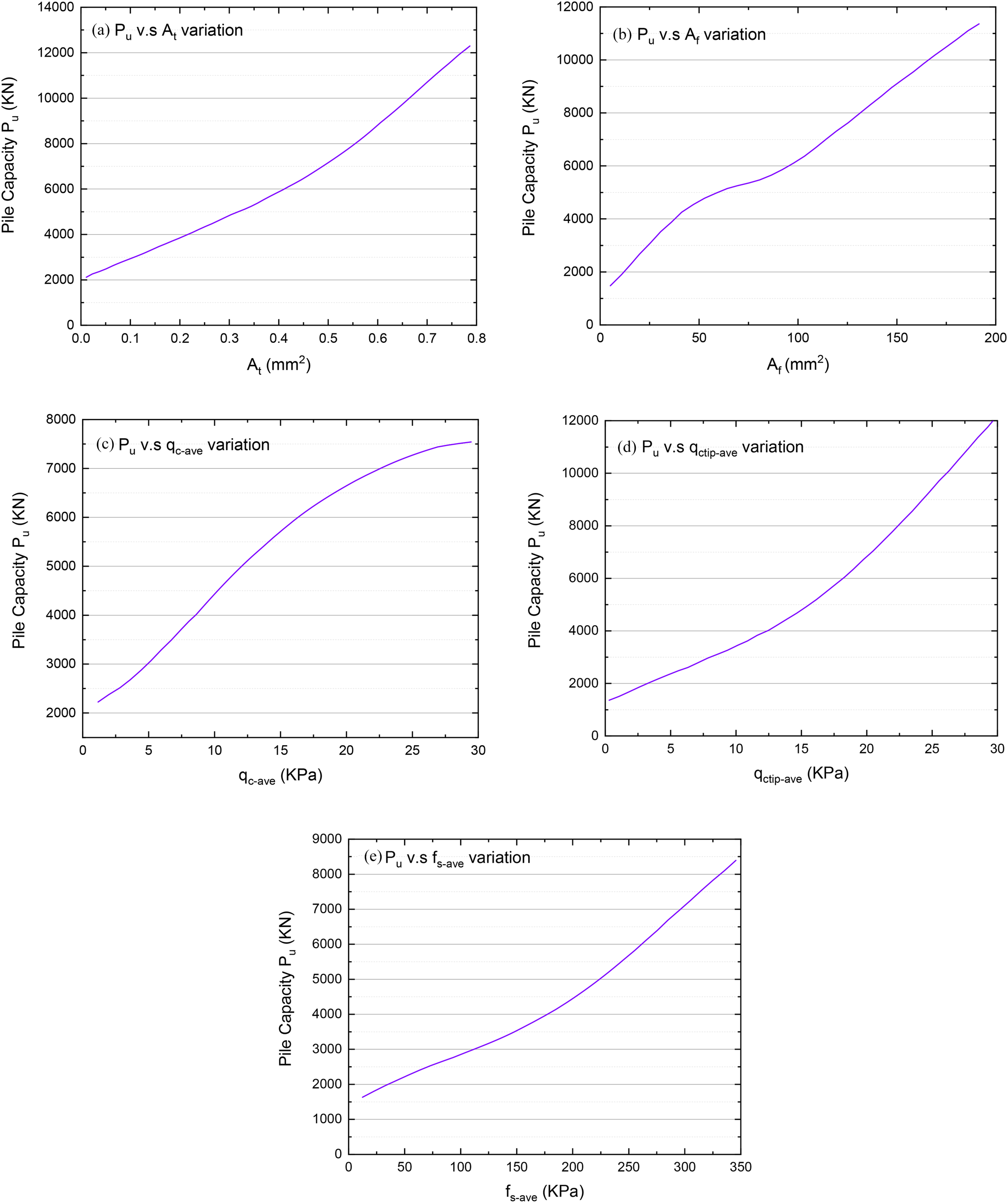
Sensitivity analysis showed the response of the hybrid ANFIS-GMDH-PSO model to each variable variation. This task performed by changing only one input variable while the remaining input variables were kept constant in their average values; therefore, an artificial data set was designed for each one of the variables with respect to its range in the data source. Then input values are introduced to the proposed ANFIS-GMDH-PSO model and finally outputs were computed. This process was repeated using remaining one or more input variables until the model response is obtained for all predictive parameters. As shown in Figure 7, the results of the sensitivity analysis confirm the fact that the ANFIS-GMDH-PSO model predicted the P u variable associated with physical behavior from an engineering perspective. It was shown that P u values were increased with increasing  $A_{\rm t}\comma \,A_{\rm s}\comma \,\bar{q}_{\rm c-{\rm shaft}}\comma \,\bar{q}_{\rm c-{\rm tip}}\comma \,\bar{f}_{\rm s}$ values individually according to Figure 7.
Sensitivity analysis of the developed ANFIS-GMDH-PSO model for P u prediction for (a)A t variable variations, (b)A s variable variations, (c) $\,\bar{q}_{\rm c-{\rm shaft}}$ variable variations, (d)
 $\bar{q}_{\rm c-{\rm tip}}$ variable variations, and (e)
 $\,\bar{f}_{\rm s}$ variable variations.

Conclusion
In this study, two different neural networks including ANFIS and GMDH techniques were combined and optimized by the PSO method in order to develop hybrid ANFIS-GMDH-PSO for predicting bearing capacity of driven piles. In this way, 108 data sets in the form of an input–output system were composed of six input variables including both coarse and fine grain soils, cone tip resistance and sleeve friction of CPTs, and geometric characterizations of piles. In the first step, the general hybrid structure of the ANFIS-GMDH model was developed and optimized using PSO. Furthermore, in the second step, three well-known empirical equations were used for comparison with the proposed AI model. The effective input parameters were involved and selected including pile and soil characteristics, PLT, and CPT results during the developed proposed model.
Comparison of the achieved results with the actual target data set showed that the hybrid ANFIS-GMDH-PSO algorithm displayed proper desired output in predicting the pile bearing capacity. In addition, this developed model showed a better performance and relative proper accuracy compared to other empirical methods established based on the CPT. The ANFIS-GMDH-PSO model does not suffer in local optimal traps by applying the PSO algorithm, and it also increases the accuracy and global search capability for ANFIS-GMDH-PSO training. This research emphasized the ability of AI-based methods to provide some more accurate methods than other analytical and empirical methods. Statistical results demonstrated that the ANFIS-GMDH-PSO models have provided better performance than other mentioned empirical CPT-based methods. Besides, results of sensitivity analysis showed that the diameter of driven pile (D) and sleeve friction (f s) parameters had the highest and lowest impacts on the bearing capacity of driven pile. Generally, performance of the integrated model of ANFIS-GMDH indicated that this soft computing tool can be employed efficiently to solve one of the most important issues in geotechnical engineering.
Dr Hooman Harandizadeh He graduated and received his Ph. D degree in Geotechnical Engineering from Shahid Bahonar University of Kerman, Iran in 2018 and he also received his MS. CE in Structural and Geotechnical Engineering from University of San Carlos, Philippine in 2010. His main interested research areas include soil and rock mechanics, pile foundation analysis and design, slope stability, soft computing modelling, and artificial intelligence methods. He has published some papers in various journals with ISI indexing. He is also reviewer of Civil engineering and AI & soft computing journals.