1. Introduction
When a thin horizontal fluid layer is heated from below and cooled from above, a density stratification appears because of the thermal expansion of the fluid. This stratification is potentially unstable: when the temperature difference between the bottom and the top exceeds a threshold value controlled by the viscosity and heat diffusivity, by a small amount, convection sets in various forms of ordered regular patterns. Since the pioneering studies of Bénard in 1900 and Rayleigh in 1916, a large number of theoretical and experimental investigations were devoted to the study of this buoyancy-driven instability. Reviews can be found in Getling (Reference Getling1988) and Bodenschatz, Pesch & Ahlers (Reference Bodenschatz, Pesch and Ahlers2000). Some of these studies were concerned with the nonlinear competition between different structures that develop above the linear convective threshold. It is found that, under Boussinesq approximations with a linear variation of the density with the temperature, rolls are stable right above onset (Schluter, Lortz & Busse Reference Schluter, Lortz and Busse1965). If the Boussinesq approximation is invalid, hexagons are preferred to rolls (Busse Reference Busse1967, Reference Busse1978) due to triad wavevector resonance. Compared with the Newtonian fluids, very few studies were devoted to non-Newtonian fluids. In the following, a literature review on convection in a horizontal layer of non-Newtonian fluid heated from below and cooled from above is presented. Most non-Newtonian fluids have two common properties: viscoelasticity and shear-thinning. Polymer and colloïd solutions as well as particulate dispersions display this behaviour above a certain concentration threshold. The influence of an elastic response, in particular the possibility of oscillatory convection due to the elastic restoring forces, has been discussed in the literature. According to Vest & Arpaci (Reference Vest and Arpaci1969), Sokolov & Tanner (Reference Sokolov and Tanner1972), Shenoy & Mashelkar (Reference Shenoy and Mashelkar1982) and Larson (Reference Larson1992), viscoelastic effects may in principle produce an oscillatory instability at a lower Rayleigh number than the Newtonian stationary mode. However, the observation of the oscillating cells requires a very high temperature difference incompatible with realistic experimental conditions (Larson Reference Larson1992). Oscillatory convection was observed for binary viscoelastic fluids, when the binary fluid aspects are significant compared with the thermal diffusion, such as in DNA suspension (Kolodner Reference Kolodner1998). The problem of pattern selection in viscoelastic fluids has also been considered in the literature, e.g. by Li & Khayat (Reference Li and Khayat2005). Using an Oldroyd-B model, they found that, near onset, rolls or hexagons can be stable, depending on secondary parameters.
Hereafter, we neglect the elastic response. We focus only on the shear-thinning effects, i.e. the influence of nonlinear decrease of the viscosity with the shear rate.
1.1. Review of Rayleigh–Bénard convection in shear-thinning fluids
To the best of the authors’ knowledge, the first experimental investigation of convection in a shear-thinning fluid layer confined between two horizontal plates was carried out by Pierre & Tien (Reference Pierre and Tien1963). The fluids used were aqueous solutions of Methocel (1 wt%) and Carbopol 934 (0.5, 0.75 and 1 wt%). The rheological behaviour of these fluids was described by a power-law model, with a shear-thinning index ranging between 0.4 and 1. The results were presented in terms of a correlation relating the Nusselt number
 $\mathit{Nu}$
to Rayleigh and Prandtl numbers, for
 $10^{5}\leqslant \mathit{Ra}\leqslant 10^{6}$
. Later on Tsuei & Tien (Reference Tsuei and Tien1973) extended this correlation to a wider range,
 $10^{3}\leqslant \mathit{Ra}\leqslant 10^{6}$
. For power-law fluids, Rayleigh and Prandtl numbers are defined with a viscosity calculated at a characteristic shear rate, which is the inverse of the thermal diffusion time. Tien, Sheng & Sun (Reference Tien, Sheng and Sun1969) attempted to establish a stability criterion for shear-thinning fluids described by a power-law model. As indicated by the authors, the linear marginal stability curve cannot be determined, because of the unphysical infinite viscosity, at zero shear rate, introduced by the rheological model. An approximate method was used for the determination of the critical Rayleigh number. It was based on the energy principle of Chandrasekhar (Reference Chandrasekhar1980): instability occurs at the minimum temperature gradient at which a balance can be steadily maintained between the kinetic energy dissipated by viscosity and the internal energy released by the buoyancy force. The solution in the limit of Newtonian fluids was used for power-law model at zero shear rate. The critical Rayleigh number was determined for two convective patterns: rolls and hexagons. The authors found that the critical Rayleigh number decreases when the shear-thinning index decreases. This evolution was also found in their experimental measurements using aqueous solutions of carboxymethylcellulose, described by a power-law model with a shear-thinning index
 $0.75\leqslant n_{p}\leqslant 1$
. Liang & Acrivos (Reference Liang and Acrivos1970) conducted an experimental study of the buoyancy-driven convection in horizontal layers of dilute aqueous solutions of polyacrylamide (Separan AP 30 at 0.5 and 1 wt%). These fluids are shear-thinning with approximately constant viscosity at low shear rate. The variation of the viscosity was about one order of magnitude over a strain-rate variation of three orders of magnitude. Liang & Acrivos (Reference Liang and Acrivos1970) found that the critical Rayleigh number is practically the same as for a Newtonian fluid and that the shear-thinning behaviour tends to increase the heat transfer.
The first numerical computation of the onset of convection in a horizontal layer of a shear-thinning fluid was done by Ozoe & Churchill (Reference Ozoe and Churchill1972). Two rheological models were considered: power-law and Ellis models. This latter model has the advantage of converging to the Newtonian behaviour in the limit of zero rate of strain. However, for certain range of rheological parameters, the viscosity in the Ellis model is not differentiable at zero shear stress. The computations were carried out for roll cells with both rigid and dragless vertical boundaries. This latter case corresponds to a roll inside a periodic row of counter-rotating rolls. The critical Rayleigh number was obtained by extrapolating the Nusselt (
 $\mathit{Nu}$
) curve to
 $\mathit{Nu}=1$
. Qualitatively, the influence of the shear thinning on the critical Rayleigh number and on the Nusselt number are similar to those obtained by Tien et al. (Reference Tien, Sheng and Sun1969). Nevertheless, the critical values found by Ozoe and Churchill are higher than those given by Tien et al. (Reference Tien, Sheng and Sun1969). The same trends were observed for rigid and dragless vertical boundaries. In a companion paper, Ozoe & Churchill (Reference Ozoe and Churchill1973) presented the computed results in terms of a correlation relating the Nusselt number to the shear-thinning index:
 $$\begin{eqnarray}\frac{\mathit{Nu}}{\mathit{Nu}_{newt}}=0.87n_{p}^{2}-2.28n_{p}+2.41,\end{eqnarray}$$
for
 $\mathit{Ra}_{c}\leqslant \mathit{Ra}\leqslant 2\mathit{Ra}_{c}$
and
 $0.5\leqslant n_{p}<1$
.
The case of very viscous fluids (infinite Prandtl number) with a power-law model and
 $0.11\leqslant n_{p}\leqslant 1$
was considered by Parmentier (Reference Parmentier1978). Numerical solutions were obtained in two-dimensional periodic convective modes. Parmentier (Reference Parmentier1978) shows that when the Rayleigh number is based on a strain-rate squared averaged viscosity, a good correlation for the heat transfer is obtained over a wide range of Rayleigh numbers. Three decades later, the two-dimensional Rayleigh–Bénard convection for a power-law fluid in a rectangular cavity with adiabatic vertical walls, was investigated numerically by Lamsaadi, Naimi & Hasnaoui (Reference Lamsaadi, Naimi and Hasnaoui2005) and Alloui et al. (Reference Alloui, Khelifa, Beji, Vasseur and Guizani2013). Their findings are qualitatively in agreement with the literature. The decrease of power-law index,
 $n$
, induces a precocious onset of convection and enhances the rate of heat transfer. Alloui et al. (Reference Alloui, Khelifa, Beji, Vasseur and Guizani2013) explain that for power-law fluids, the system is unconditionally stable to infinitesimal disturbances. Note that Lamsaadi et al. (Reference Lamsaadi, Naimi and Hasnaoui2005) and Alloui et al. (Reference Alloui, Khelifa, Beji, Vasseur and Guizani2013) considered a shallow rectangular cavity heated and cooled with uniform heat fluxes. In this case, the system convects with one cell. Relying on a parallel flow concept for infinite aspect ratio, Alloui et al. (Reference Alloui, Khelifa, Beji, Vasseur and Guizani2013) show that the onset of convection occurs at subcritical Rayleigh number.
Weakly nonlinear stability analysis of thermal convection for shear-thinning fluid between two plates maintained at different temperatures was performed by Balmforth & Rust (Reference Balmforth and Rust2009). Assuming a two-dimensional situation, with stress-free boundary conditions (SFBCs), the authors found that when the degree of shear-thinning
 ${\it\alpha}=|\text{d}{\it\mu}/\text{d}{\it\Gamma}|_{{\it\Gamma}=0}$
is greater than
 $24/(601{\rm\pi}^{4})$
the bifurcation becomes subcritical. In the previous expression, the viscosity
 ${\it\mu}$
and the second invariant of the strain rate deformation
 ${\it\Gamma}$
(defined by (2.7)) are rendered dimensionless using the zero-shear-rate viscosity and thermal-diffusion time as characteristic scales. Recently, a systematic weakly nonlinear analysis for Carreau fluid in two- and three-dimensional situations with SFBC was carried out by Albaalbaki & Khayat (Reference Albaalbaki and Khayat2011). When the convection takes place in the form of rolls, the threshold value of
 ${\it\alpha}$
for a subcritical bifurcation found was
 $14\times 10^{-4}$
, in disagreement with Balmforth & Rust (Reference Balmforth and Rust2009). Albaalbaki & Khayat (Reference Albaalbaki and Khayat2011) found also that depending on the degree of shear-thinning, the fluid can convect in the form of rolls, squares or hexagons. This result is surprising. Usually, near the onset of convection, hexagons are observed in convection systems lacking midplane reflection symmetry such as in fluids with strongly temperature-dependent viscosity (Palm Reference Palm1960; Golubitsky, Swift & Knoblock Reference Golubitsky, Swift and Knoblock1984) or in Bénard–Marangoni convection (Thess & Bestehorn Reference Thess and Bestehorn1995). Indeed, in such systems, quadratic terms present in amplitude equations enable triadic resonant wavevector interactions that can explain the occurrence of hexagons near onset. In § 5.5.4, it will be shown that under Boussinesq approximations, with identical boundary conditions at the two horizontal plates, the non-Newtonian terms do not break the midplane reflection.
1.2. Objectives, methodology and outline of the paper
Here, we consider shear-thinning fluids with a finite zero-shear-rate viscosity
 ${\it\mu}_{0}$
. The Carreau (Reference Carreau1972) model (2.8) is adopted to describe the nonlinear variation of the viscosity
 ${\it\mu}$
with the second invariant of the strain-rate tensor
 ${\it\Gamma}$
. This model is chosen because it has a sound theoretical basis, and is
 $C^{\infty }$
with respect to
 ${\it\Gamma}$
, unlike the power-law model or the general Carreau–Yasuda model, which are singular at
 ${\it\Gamma}=0$
. Interestingly, the Carreau model approaches the power-law model, as the viscosity
 ${\it\mu}_{0}$
or the characteristic time
 ${\it\lambda}$
of the fluid become large.
In light of the previous works, there are two points that need to be re-examined. The first one concerns the critical value of the degree of shear-thinning,
 ${\it\alpha}$
, above which the bifurcation becomes subcritical. This value was determined only for SFBCs which are not quite physical, and moreover the existing results are contradictory. The second point concerns the competition between different patterns of convection near the criticality. Only Albaalbaki & Khayat (Reference Albaalbaki and Khayat2011) dealt with this problem, using SFBCs.
The purpose of the present work is to revisit the Rayleigh–Bénard problem for shear-thinning fluids using more general boundary conditions, with both slip and stress, i.e. Navier-type boundary conditions with a slip parameter. Note that, for Newtonian fluids with Navier slip boundary conditions, only the linear stability of the Rayleigh–Bénard problem has been studied by Webber (Reference Webber2006) and Kuo & Chen (Reference Kuo and Chen2009). Here, a general weakly nonlinear analysis is performed. The calculation of the saturation coefficient at the cubic order allows one to determine the nature of the bifurcation depending on the slip and rheological parameters. The study of the stability of fixed points of amplitude equations allows one to analyse the competition between different convection patterns near onset. Then, we examine the relevance of the principle of maximum heat transfer for non-Newtonian fluids. Calculation at higher order allows one to characterize the convection for a significant departure from the critical conditions, in particular, through a correlation for the Nusselt number using a generalized Rayleigh number as suggested by Parmentier (Reference Parmentier1978).
The article is organized as follows. In § 2, the governing equations of mass, momentum and energy are presented in dimensionless form. Section 3 deals with the linear stability theory. The influence of the slip parameter on the critical Rayleigh number and critical wavenumber is examined. In § 4, the main steps of the weakly nonlinear analysis are outlined. The results are presented and discussed in § 5. The nature of the bifurcation is determined and the competition between different patterns near onset is analysed. It is found that only rolls are stable. This result is confirmed in § 6, by computing higher-order Landau constants. The flow structure, the modification of the viscosity field and the heat transfer for steady rolls are described in § 7. Finally, § 8 is devoted to a concluding discussion.
2. Physical and mathematical model
2.1. General equations and parameters
Hereafter, quantities with hats are dimensional quantities. We consider a layer of shear-thinning fluid of depth
 $\hat{d}$
confined between two horizontal plates, infinite in extent, which are perfect heat conductors. The bottom and top plates are kept at constant temperatures, respectively
 $\hat{T}_{0}+{\it\delta}\hat{T}/2$
and
 $\hat{T}_{0}-{\it\delta}\hat{T}/2$
, with
 ${\it\delta}\hat{T}>0$
. The fluid has density
 $\hat{{\it\rho}}$
, thermal diffusivity
 $\hat{{\it\kappa}}$
, thermal expansion coefficient
 $\hat{{\it\beta}}$
and viscosity
 $\hat{{\it\mu}}_{0}$
at zero shear rate. Because of the thermal expansion, the temperature difference between the two plates induces a vertical density stratification. Heavy cold fluid is above a light warm fluid. For small
 ${\it\delta}\hat{T}$
, the fluid remains at rest and the heat is transferred by conduction. The hydrostatic solution for the pressure
 $\hat{P}$
and the temperature profile are
 $$\begin{eqnarray}\frac{\text{d}\hat{P}}{\text{d}\hat{z}}=-\hat{{\it\rho}}_{0}{\hat{g}}\left[1-\hat{{\it\beta}}\left(\hat{T}-\hat{T}_{0}\right)\right]\quad \text{and}\quad \hat{T}_{cond}-\hat{T}_{0}=\frac{{\it\delta}\hat{T}}{2}\left(1-\frac{2\hat{z}}{\hat{d}}\right),\end{eqnarray}$$
with
 $\hat{{\it\rho}}_{0}$
the fluid density at the reference temperature and
 ${\hat{g}}$
the acceleration due to gravity. The
 $z$
-axis is directed upwards, with its origin located at the bottom plate. The stability of the hydrostatic solution is considered by introducing temperature and pressure perturbation as well as a fluid motion. Boussinesq approximation is adopted, i.e. the temperature dependence of the fluid properties can be neglected except for the temperature-induced density difference in the buoyancy force. The heat production due to viscosity is neglected. Using the units
 $\hat{d}^{2}/\hat{{\it\kappa}}$
,
 $\hat{d}$
,
 $\hat{{\it\kappa}}/\hat{d}$
and
 ${\rm\Delta}\hat{T}$
for time, length, velocity and temperature, the dimensionless perturbation equations are
 $$\begin{eqnarray}\displaystyle & \boldsymbol{{\rm\nabla}}\boldsymbol{\cdot }\boldsymbol{u}=0, & \displaystyle\end{eqnarray}$$
 $$\begin{eqnarray}\displaystyle & \displaystyle \frac{1}{\mathit{Pr}}\left[\frac{\partial \boldsymbol{u}}{\partial t}+\left(\boldsymbol{u}\boldsymbol{\cdot }\boldsymbol{{\rm\nabla}}\right)\boldsymbol{u}\right]=-\boldsymbol{{\rm\nabla}}p+\mathit{Ra}{\it\theta}\boldsymbol{e}_{z}+\boldsymbol{{\rm\nabla}}\boldsymbol{\cdot }{\bf\tau}, & \displaystyle\end{eqnarray}$$
 $$\begin{eqnarray}\displaystyle & \displaystyle \frac{\partial {\it\theta}}{\partial t}+\boldsymbol{u}\boldsymbol{\cdot }\boldsymbol{{\rm\nabla}}{\it\theta}=\boldsymbol{u}\boldsymbol{\cdot }\boldsymbol{e}_{z}+{\rm\nabla}^{2}{\it\theta}. & \displaystyle\end{eqnarray}$$
 $\boldsymbol{e}_{z}$
denotes the unit vector in the vertical direction,
 $\boldsymbol{u}(\boldsymbol{x},t)$
the fluid velocity,
 $p(\boldsymbol{x},t)$
and
 ${\it\theta}(\boldsymbol{x},t)$
represent the pressure and temperature deviations from their values in the conductive state. We denote
 $(x,y,z)$
as the components of the position vector
 $\boldsymbol{x}$
, and
 $(u,v,w)$
the components of the velocity vector
 $\boldsymbol{u}$
. The Rayleigh number
 $\mathit{Ra}$
and the Prandtl number
 $\mathit{Pr}$
are
 $$\begin{eqnarray}\mathit{Ra}=\frac{\hat{{\it\rho}}_{0}{\hat{g}}\hat{{\it\beta}}{\it\delta}\hat{T}\hat{d}^{3}}{\hat{{\it\kappa}}\hat{{\it\mu}}_{0}},\quad \mathit{Pr}=\frac{\hat{{\it\mu}}_{0}}{\hat{{\it\rho}}_{0}\hat{{\it\kappa}}}.\end{eqnarray}$$
In general, for non-Newtonian fluids,
 $\mathit{Pr}\gg 1$
, i.e. the viscous diffusion time is shorter than the thermal diffusion time.
2.2. Rheological model and parameters
The fluid is assumed to be purely viscous and shear-thinning. The viscous stress tensor
 $$\begin{eqnarray}{\bf\tau}={\it\mu}\left({\it\Gamma}\right)\dot{{\bf\gamma}}\quad \text{with}~\dot{{\bf\gamma}}=\boldsymbol{{\rm\nabla}}\boldsymbol{u}+\left(\boldsymbol{{\rm\nabla}}\boldsymbol{u}\right)^{\text{T}}\end{eqnarray}$$
the rate-of-strain tensor, of second invariant
 $$\begin{eqnarray}{\it\Gamma}={\textstyle \frac{1}{2}}\dot{{\it\gamma}}_{ij}\dot{{\it\gamma}}_{ij}.\end{eqnarray}$$
The Carreau model is given by
 $$\begin{eqnarray}\frac{\hat{{\it\mu}}-\hat{{\it\mu}}_{\infty }}{\hat{{\it\mu}}_{0}-\hat{{\it\mu}}_{\infty }}=\left(1+\hat{{\it\lambda}}^{2}\hat{{\it\Gamma}}\right)^{(n_{c}-1)/2},\end{eqnarray}$$
with
 $\hat{{\it\mu}}_{0}$
and
 $\hat{{\it\mu}}_{\infty }$
the viscosities at low and high shear rate,
 $(n_{c}<1)$
, the shear-thinning index and
 $\hat{{\it\lambda}}$
the characteristic time of the fluid. The location of the transition from the Newtonian plateau to the shear-thinning regime is determined by
 $\hat{{\it\lambda}}$
, since
 $1/\hat{{\it\lambda}}$
defines the characteristic shear rate for the onset of shear-thinning. Increasing
 $\hat{{\it\lambda}}$
reduces the Newtonian plateau to lower shear rates. The infinite shear viscosity,
 $\hat{{\it\mu}}_{\infty }$
, is generally associated with a breakdown of the fluid, and is frequently significantly smaller (
 $10^{-3}{-}10^{-4}$
times smaller) than
 $\hat{{\it\mu}}_{0}$
, see Bird, Amstrong & Hassager (Reference Bird, Amstrong and Hassager1987) and Tanner (Reference Tanner2000). The ratio
 $\hat{{\it\mu}}_{\infty }/\hat{{\it\mu}}_{0}$
will be thus neglected in the following. The dimensionless effective viscosity is then
 $$\begin{eqnarray}{\it\mu}=\frac{\hat{{\it\mu}}}{\hat{{\it\mu}}_{0}}=\left(1+{\it\lambda}^{2}{\it\Gamma}\right)^{(n_{c}-1)/2}\quad \text{with}~{\it\lambda}=\frac{\hat{{\it\lambda}}}{\hat{d}^{2}/\hat{{\it\kappa}}}.\end{eqnarray}$$
The Newtonian behaviour,
 $\hat{{\it\mu}}=\hat{{\it\mu}}_{0}$
, is obtained by setting
 $n_{c}=1$
or
 $\hat{{\it\lambda}}=0$
.
For a small-amplitude disturbance, the viscosity can be expanded about the hydrostatic solution,
 $$\begin{eqnarray}{\it\mu}=1+\left(\frac{n_{c}-1}{2}\right){\it\lambda}^{2}{\it\Gamma}+\frac{1}{2}\left(\frac{n_{c}-1}{2}\right)\left(\frac{n_{c}-3}{2}\right){\it\lambda}^{4}{\it\Gamma}^{2}+\cdots .\end{eqnarray}$$
At lowest nonlinear order, a relevant rheological parameter is the ‘degree of shear-thinning’
 $$\begin{eqnarray}{\it\alpha}=\left|\frac{\text{d}{\it\mu}}{\text{d}{\it\Gamma}}\right|_{{\it\Gamma}=0}=\frac{1-n_{c}}{2}{\it\lambda}^{2}.\end{eqnarray}$$
2.3. Boundary conditions with slip
The plates are not permeable, i.e.
 $$\begin{eqnarray}\boldsymbol{u}\boldsymbol{\cdot }\boldsymbol{n}=0,\end{eqnarray}$$
 $\boldsymbol{n}$
being the unit vector normal to the wall, pointing towards the fluid. Concerning the component of the fluid velocity tangent to the plates, it can be significantly affected by liquid–surface wall interactions. Polymer melts and solutions usually slip at a plane wall (Denn Reference Denn2001). This slip may result from an adhesive failure of the polymer chains at the solid surface or from disentanglement between chains adsorbed to the wall and those in the polymer bulk (Brochard & de Gennes Reference Brochard and de Gennes1992; Baljon & Robbins Reference Baljon and Robbins1997). Another class of complex fluids prone to wall slip are colloidal suspensions and emulsions. In this case, slip arises from a depletion of particles adjacent to the shearing surfaces (Barnes Reference Barnes1995). The wall slip is often modelled macroscopically using Navier’s slip law. This law is adopted in the present study, to take into account of a possible wall slip. For purely viscous non-Newtonian fluids, the tangent velocity
 $\boldsymbol{u}_{t}$
is proportional to the tangent wall shear stress
 ${\bf\tau}_{t}$
via an empirical coefficient
 $L_{s}$
, called the slip parameter (Ferras, Nobrega & Pinho Reference Ferras, Nobrega and Pinho2012):
 $$\begin{eqnarray}\boldsymbol{u}_{t}=L_{s}{\bf\tau}_{t},\end{eqnarray}$$
with
 $\boldsymbol{u}_{t}=\boldsymbol{u}-(\boldsymbol{u}\boldsymbol{\cdot }\boldsymbol{n})\boldsymbol{n}$
,
 ${\bf\tau}_{t}={\bf\tau}\boldsymbol{\cdot }\boldsymbol{n}-{\it\tau}_{n}\boldsymbol{n}$
and
 ${\it\tau}_{n}=\boldsymbol{n}\boldsymbol{\cdot }{\bf\tau}\boldsymbol{\cdot }\boldsymbol{n}$
. No-slip boundary conditions (NSBCs) are recovered by setting
 $L_{s}=0$
. SFBCs are recovered in the limit
 $L_{s}\rightarrow +\infty$
. As can be seen in (2.21) below, the product
 $L_{s}{\it\mu}$
can be seen as a ‘slip length’. Hereafter,
 $L_{s}$
is assumed to be a constant parameter, that depends only on the precise nature of the interface and of the fluid.
For the temperature, as already stated,
 $$\begin{eqnarray}{\it\theta}=0\quad \text{at}~z=0,1.\end{eqnarray}$$
2.4. Midplane reflection or ‘Boussinesq’ symmetry
The governing equations (2.3), (2.4) with the constitutive equation (2.6) and the boundary conditions (2.12)–(2.14) are reflection-symmetric about the midplane
 $z=1/2$
. The action of this so-called Boussinesq symmetry is
 $$\begin{eqnarray}\left[u,v,w,{\it\theta},p\right](t,x,y,z)\rightarrow \left[u,v,-w,{\it\theta},p\right](t,x,y,1-z).\end{eqnarray}$$
This symmetry plays an essential role in the pattern selection.
2.5. Reduction: elimination of the pressure
The pressure field is eliminated by applying the curl to (2.3). Then, we take curl curl of (2.3). Using the continuity equation, and projecting onto
 $\boldsymbol{e}_{z}$
, we get the following evolution equations for the vertical vorticity
 ${\it\zeta}=\partial v/\partial x-\partial u/\partial y$
and the vertical velocity
 $w$
:
 $$\begin{eqnarray}\frac{1}{\mathit{Pr}}\left[\frac{\partial {\it\zeta}}{\partial t}+\boldsymbol{e}_{z}\boldsymbol{\cdot }\boldsymbol{{\rm\nabla}}\times \left[\left(\boldsymbol{u}\boldsymbol{\cdot }\boldsymbol{{\rm\nabla}}\right)\boldsymbol{u}\right]\right]={\rm\Delta}{\it\zeta}+\boldsymbol{e}_{z}\boldsymbol{\cdot }\boldsymbol{{\rm\nabla}}\times [\boldsymbol{{\rm\nabla}}\boldsymbol{\cdot }({\it\mu}-1)\dot{{\bf\gamma}}],\end{eqnarray}$$
 $$\begin{eqnarray}\displaystyle & & \displaystyle \frac{1}{\mathit{Pr}}\left[\frac{\partial {\rm\Delta}w}{\partial t}-\boldsymbol{e}_{z}\boldsymbol{\cdot }\left[\boldsymbol{{\rm\nabla}}\times \boldsymbol{{\rm\nabla}}\times \left(\left(\boldsymbol{u}\boldsymbol{\cdot }\boldsymbol{{\rm\nabla}}\right)\boldsymbol{u}\right)\right]\right]\nonumber\\ \displaystyle & & \displaystyle \quad ={\it\Delta}^{2}w+\mathit{Ra}{\it\Delta}_{H}{\it\theta}-\left[\boldsymbol{{\rm\nabla}}\times \boldsymbol{{\rm\nabla}}\times \left[\boldsymbol{{\rm\nabla}}\boldsymbol{\cdot }({\it\mu}-1)\dot{{\bf\gamma}}\right]\right]\boldsymbol{\cdot }\boldsymbol{e}_{z},\end{eqnarray}$$
 $$\begin{eqnarray}\frac{\partial {\it\theta}}{\partial t}+\boldsymbol{u}\boldsymbol{\cdot }\boldsymbol{{\rm\nabla}}{\it\theta}=w+{\rm\Delta}{\it\theta},\end{eqnarray}$$
where the ‘horizontal Laplacian’
 $$\begin{eqnarray}{\it\Delta}_{H}=\frac{\partial ^{2}}{\partial x^{2}}+\frac{\partial ^{2}}{\partial y^{2}}.\end{eqnarray}$$
From the continuity equation and the vertical vorticity definition, one deduces the horizontal velocity components:
 $$\begin{eqnarray}{\it\Delta}_{H}u=-\frac{\partial ^{2}w}{\partial x\partial z}-\frac{\partial {\it\zeta}}{\partial y};\quad {\it\Delta}_{H}v=-\frac{\partial ^{2}w}{\partial y\partial z}+\frac{\partial {\it\zeta}}{\partial x}.\end{eqnarray}$$
The boundary conditions are
 $$\begin{eqnarray}\displaystyle & \displaystyle w=0,\quad {\it\theta}=0,\quad u=L_{s}{\it\mu}\frac{\partial u}{\partial z},\quad v=L_{s}{\it\mu}\frac{\partial v}{\partial z},\quad \text{at}~z=0, & \displaystyle\end{eqnarray}$$
 $$\begin{eqnarray}\displaystyle & \displaystyle w=0,\quad {\it\theta}=0,\quad u=-L_{s}{\it\mu}\frac{\partial u}{\partial z},\quad v=-L_{s}{\it\mu}\frac{\partial v}{\partial z},\quad \text{at}~z=1. & \displaystyle\end{eqnarray}$$
 $x$
and
 $y$
, to obtain the equivalent conditions
 $$\begin{eqnarray}\displaystyle & \displaystyle \frac{\partial w}{\partial z}=L_{s}\left({\it\mu}\frac{\partial ^{2}w}{\partial z^{2}}-\frac{\partial {\it\mu}}{\partial x}\frac{\partial u}{\partial z}-\frac{\partial {\it\mu}}{\partial y}\frac{\partial v}{\partial z}\right), & \displaystyle\end{eqnarray}$$
 $$\begin{eqnarray}\displaystyle & \displaystyle {\it\zeta}=L_{s}\left[{\it\mu}\frac{\partial {\it\zeta}}{\partial z}+\left(\frac{\partial {\it\mu}}{\partial x}\frac{\partial v}{\partial z}-\frac{\partial {\it\mu}}{\partial y}\frac{\partial u}{\partial z}\right)\right],\quad \text{at}~z=0, & \displaystyle\end{eqnarray}$$
 $$\begin{eqnarray}\displaystyle & \displaystyle \frac{\partial w}{\partial z}=-L_{s}\left({\it\mu}\frac{\partial ^{2}w}{\partial z^{2}}-\frac{\partial {\it\mu}}{\partial x}\frac{\partial u}{\partial z}-\frac{\partial {\it\mu}}{\partial y}\frac{\partial v}{\partial z}\right), & \displaystyle\end{eqnarray}$$
 $$\begin{eqnarray}\displaystyle & \displaystyle {\it\zeta}=-L_{s}\left[{\it\mu}\frac{\partial {\it\zeta}}{\partial z}+\left(\frac{\partial {\it\mu}}{\partial x}\frac{\partial v}{\partial z}-\frac{\partial {\it\mu}}{\partial y}\frac{\partial u}{\partial z}\right)\right],\quad \text{at}~z=1. & \displaystyle\end{eqnarray}$$
3. Linear stability analysis
3.1. Direct eigenvalue problem: critical conditions
In the linear theory,
 $\boldsymbol{u}$
and
 ${\it\theta}$
are assumed to be infinitesimal. By neglecting the nonlinear terms in (2.16)–(2.18), one obtains the linear problem:
 $$\begin{eqnarray}\displaystyle & \displaystyle \frac{1}{\mathit{Pr}}\frac{\partial {\it\zeta}}{\partial t}={\rm\Delta}{\it\zeta}, & \displaystyle\end{eqnarray}$$
 $$\begin{eqnarray}\displaystyle & \displaystyle \frac{1}{\mathit{Pr}}\frac{\partial {\rm\Delta}w}{\partial t}={\it\Delta}^{2}w+\mathit{Ra}{\it\Delta}_{H}{\it\theta}, & \displaystyle\end{eqnarray}$$
 $$\begin{eqnarray}\displaystyle & \displaystyle \frac{\partial {\it\theta}}{\partial t}=w+{\rm\Delta}{\it\theta}. & \displaystyle\end{eqnarray}$$
 $$\begin{eqnarray}\left[\begin{array}{@{}c@{}}w(x,y,z,t)\\ {\it\theta}(x,y,z,t)\end{array}\right]=\left[\begin{array}{@{}c@{}}F_{11}(z)\\ G_{11}(z)\end{array}\right]f(x,y)\exp (st),\end{eqnarray}$$
with
 $f(x,y)=\exp (\text{i}k_{x}x+\text{i}k_{y}y)$
,
 $\boldsymbol{k}=(k_{x},k_{y},0)$
the horizontal wavenumber and
 $s=s_{r}+\text{i}s_{i}$
a complex number. This leads to the differential equations
 $$\begin{eqnarray}\displaystyle & s\mathit{Pr}^{-1}(D^{2}-k^{2})F_{11}=-k^{2}\mathit{Ra}G_{11}+(D^{2}-k^{2})^{2}F_{11}, & \displaystyle\end{eqnarray}$$
 $$\begin{eqnarray}\displaystyle & sG_{11}=F_{11}+(D^{2}-k^{2})G_{11}, & \displaystyle\end{eqnarray}$$
 $D$
the derivative with respect to
 $z$
and
 $k$
the norm of the vector
 $\boldsymbol{k}$
. The boundary conditions are
 $$\begin{eqnarray}\displaystyle & F_{11}=0,\quad DF_{11}-L_{s}D^{2}F_{11}=0,\quad G_{11}=0\quad \text{at}~z=0, & \displaystyle\end{eqnarray}$$
 $$\begin{eqnarray}\displaystyle & F_{11}=0,\quad DF_{11}+L_{s}D^{2}F_{11}=0,\quad G_{11}=0\quad \text{at}~z=1. & \displaystyle\end{eqnarray}$$
 $s_{i}=0$
, when Navier’s slip boundary conditions are used. The set of differential equations (3.5) and (3.6) is an eigenvalue problem where
 $s$
is the eigenvalue and
 $\boldsymbol{X}_{11}=(F_{11},G_{11})$
the eigenvector. It can be written
 $$\begin{eqnarray}s\boldsymbol{M}\boldsymbol{\cdot }\boldsymbol{X}_{11}=\boldsymbol{L}\boldsymbol{\cdot }\boldsymbol{X}_{11}.\end{eqnarray}$$
Since any multiple of the eigenvector
 $\boldsymbol{X}_{11}$
is also a solution of (3.8), and for symmetry reasons,
 $\boldsymbol{X}_{11}$
can be normalized such that
 $$\begin{eqnarray}G_{11}(z=1/2)=1.\end{eqnarray}$$
A spectral Chebyshev method is used. The eigenfunctions
 $F_{11}$
and
 $G_{11}$
are expanded in terms of the Chebyshev polynomials,
 $T_{j}$
,
 $$\begin{eqnarray}F_{11}(z)=\mathop{\sum }_{j=0}^{N}a_{j}T_{j}\left(2z-1\right),\quad G_{11}(z)=\mathop{\sum }_{j=0}^{N}b_{j}T_{j}\left(2z-1\right).\end{eqnarray}$$
By cancelling the residual
 $(s\boldsymbol{M}\boldsymbol{\cdot }\boldsymbol{X}_{11}-\boldsymbol{L}\boldsymbol{\cdot }\boldsymbol{X}_{11})$
at the
 $(N+1)$
collocation points (Gauss–Lobatto points)
 $z_{j}=(\cos ({\rm\pi}j/N)+1)/2$
, for
 $j=0,1,\dots ,N$
, one obtains a matrix eigenvalue problem solved using the QZ algorithm with Matlab. The marginal stability curve
 $\mathit{Ra}(k)$
is obtained by the condition
 $s(\mathit{Ra},k)=0$
. Using 20 Chebyshev polynomials, the first eigenvalue, i.e. that for which the real part is the largest, is calculated with an accuracy of
 $10^{-4}$
. The minimum of the marginal stability curves gives the critical Rayleigh number
 $\mathit{Ra}_{c}$
and critical wavenumber
 $k_{c}$
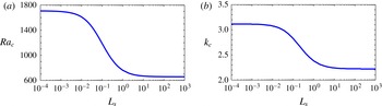
. Figure 1 displays the variation of
 $\mathit{Ra}_{c}$
and
 $k_{c}$
as a function of the dimensionless slip parameter. These results are in very good quantitative agreement with those obtained by Webber (Reference Webber2006) and Kuo & Chen (Reference Kuo and Chen2009). The critical Rayleigh number decreases with increasing slip parameter
 $L_{s}$
, from 1707.7 (NSBCs) to
 $27{\rm\pi}^{4}/4=657.5$
(SFBCs). The slip has therefore a destabilizing effect. The critical wavenumber decreases with increasing
 $L_{s}$
, from 3.116 (NSBCs) to
 ${\rm\pi}/\sqrt{2}=2.221$
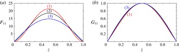
(SFBCs). Additional properties of the critical mode are given by
 $F_{11}$
and
 $G_{11}$
at the critical conditions. They are displayed in figure 2 for different values of
 $L_{s}$
. Here,
 $F_{11}(z)$
and
 $G_{11}(z)$
are real-valued functions. The critical mode is such that
 $w$
and
 ${\it\theta}$
are even with respect to the midplane reflection symmetry. Hence, according to (2.20),
 $u$
and
 $v$
are odd. For SFBCs, the critical mode is obtained analytically:
 $$\begin{eqnarray}w=\frac{3{\rm\pi}^{2}}{2}\sin \left({\rm\pi}z\right)f(x,y),\quad {\it\theta}=\sin ({\rm\pi}z)f(x,y),\end{eqnarray}$$
 $$\begin{eqnarray}u=3{\rm\pi}\cos ({\rm\pi}z)\frac{\partial f}{\partial x},\quad v=3{\rm\pi}\cos ({\rm\pi}z)\frac{\partial f}{\partial y}.\end{eqnarray}$$
Critical Rayleigh number (a) and critical wavenumber (b) as a function of the slip parameter.

Eigenfunctions at critical conditions and different values of
 $L_{s}$
: (1)
 $L_{s}=0$
, i.e. NSBC; (2)
 $L_{s}=0.1$
; and (3)
 $L_{s}=10^{4}$
very close to SFBC.

3.2. Adjoint eigenvalue problem: adjoint mode
For vectors fields
 $\boldsymbol{f}$
and
 $\boldsymbol{g}$
, one defines a scalar product by
 $$\begin{eqnarray}\left\langle \boldsymbol{f},\boldsymbol{g}\right\rangle =\int _{0}^{1}\boldsymbol{f}\boldsymbol{\cdot }\boldsymbol{g}\,\text{d}z.\end{eqnarray}$$
To the direct problem (3.8) corresponds the adjoint problem
 $$\begin{eqnarray}s\boldsymbol{M}^{+}\boldsymbol{\cdot }\boldsymbol{X}_{\boldsymbol{ad}}=\boldsymbol{L}^{+}\boldsymbol{\cdot }\boldsymbol{X}_{\boldsymbol{ad}}\quad \text{with}~\boldsymbol{X}_{ad}=(F_{ad},G_{ad}),\end{eqnarray}$$
where the adjoint operators
 $\boldsymbol{M}^{+}$
and
 $\boldsymbol{L}^{+}$
are defined by
 $$\begin{eqnarray}\left\langle \boldsymbol{X}_{ad},\boldsymbol{M}\boldsymbol{\cdot }\boldsymbol{X}\right\rangle =\left\langle \boldsymbol{M}^{+}\boldsymbol{\cdot }\boldsymbol{X}_{ad},\boldsymbol{X}\right\rangle ,\quad \left\langle \boldsymbol{X}_{ad},\boldsymbol{L}\boldsymbol{\cdot }\boldsymbol{X}\right\rangle =\left\langle \boldsymbol{L}^{+}\boldsymbol{\cdot }\boldsymbol{X}_{ad},\boldsymbol{X}\right\rangle \!,\end{eqnarray}$$
where
 $\boldsymbol{X}$
fulfills the ‘linear’ boundary conditions (3.7). By integrating by parts we get the linear adjoint problem and the corresponding boundary conditions
 $$\begin{eqnarray}\displaystyle & s\mathit{Pr}^{-1}\left(D^{2}-k^{2}\right)F_{ad}=\left(D^{2}-k^{2}\right)^{2}F_{ad}+G_{ad}, & \displaystyle\end{eqnarray}$$
 $$\begin{eqnarray}\displaystyle & sG_{ad}=-k^{2}\mathit{Ra}F_{ad}+\left(D^{2}-k^{2}\right)G_{ad}, & \displaystyle\end{eqnarray}$$
 $$\begin{eqnarray}\displaystyle & F_{ad}=0,\quad DF_{ad}-L_{s}D^{2}F_{ad}=0,\quad G_{ad}=0\quad \text{at}~z=0, & \displaystyle\end{eqnarray}$$
 $$\begin{eqnarray}\displaystyle & F_{ad}=0,\quad DF_{ad}+L_{s}D^{2}F_{ad}=0,\quad G_{ad}=0\quad \text{at}~z=1. & \displaystyle\end{eqnarray}$$
 $$\begin{eqnarray}G_{ad}\left(z=1/2\right)=1.\end{eqnarray}$$
At
 $\mathit{Ra}=\mathit{Ra}_{c}$
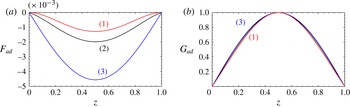
, the so-called adjoint critical mode does not depend on the Prandtl number. It is displayed in figure 3 for three values of the slip parameter. For SFBCs, the critical adjoint mode is given by
 $$\begin{eqnarray}w^{+}=-\frac{4}{9{\rm\pi}^{4}}\text{sin}({\rm\pi}z)f(x,y),\quad {\it\theta}^{+}=\sin ({\rm\pi}z)f(x,y),\end{eqnarray}$$
 $$\begin{eqnarray}u^{+}=-\frac{8}{9{\rm\pi}^{5}}\cos ({\rm\pi}z)\frac{\partial f}{\partial x},\quad v^{+}=-\frac{8}{9{\rm\pi}^{5}}\cos ({\rm\pi}z)\frac{\partial f}{\partial y}.\end{eqnarray}$$
Note that
 $F_{ad}$
is three order of magnitude smaller than
 $G_{ad}$
. This indicates that the system is more receptive to thermal perturbations than to velocity perturbations.
Adjoint functions at critical conditions, and different values of
 $L_{s}$
: (1)
 $L_{s}=0$
(NSBC); (2)
 $L_{s}=0.1$
; and (3)
 $L_{s}=10^{4}$
very close to SFBC.

3.3. Characteristic time of the instability
In slightly supercritical conditions, the growth rate
 $s$
can be approximated using Taylor expansion,
 $$\begin{eqnarray}s=\frac{{\it\epsilon}}{{\it\tau}_{0}}+O({\it\epsilon}^{2})\quad \text{with}~{\it\epsilon}=\frac{\mathit{Ra}-\mathit{Ra}_{c}}{\mathit{Ra}_{c}}.\end{eqnarray}$$
The determination of the characteristic time
 ${\it\tau}_{0}$
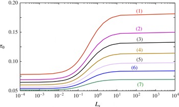
of the instability follows the methodology described in Cross (Reference Cross1980). The details are given in appendix A. Figure 4 shows the variation of
 ${\it\tau}_{0}$
as a function of
 $L_{s}$
for different values of
 $\mathit{Pr}$
. It increases from
 $$\begin{eqnarray}{\it\tau}_{0}=\frac{1+1.9544\mathit{Pr}}{38.4429\mathit{Pr}}\end{eqnarray}$$
for NSBCs (Segel Reference Segel1969; Cross Reference Cross1980; Daniels & Ong Reference Daniels and Ong1990) to
 $$\begin{eqnarray}{\it\tau}_{0}=\frac{2}{3{\rm\pi}^{2}}\frac{1+\mathit{Pr}}{\mathit{Pr}}\end{eqnarray}$$
for SFBCs (Newell & Whitehead Reference Newell and Whitehead1969). The effect of
 $L_{s}$
is all the more significant when the Prandtl number is low.
Characteristic time of instability as a function of
 $L_{s}$
for different Prandtl numbers: (1)
 $\mathit{Pr}=1$
; (2)
 $\mathit{Pr}=1.5$
; (3)
 $\mathit{Pr}=2$
; (4)
 $\mathit{Pr}=3$
; (5)
 $\mathit{Pr}=5$
;(6)
 $\mathit{Pr}=10$
; (7)
 $\mathit{Pr}=100$
.

4. Weakly nonlinear stability analysis: formulation and procedure
For given boundary conditions, the critical Rayleigh number for the onset of convection, determined from the linear stability analysis, depends only on the norm
 $k_{c}$
of the wavevector. Because of the isotropy of the extended horizontal plane, the direction of the wavevector is arbitrary. In addition, any linear combination of modes
 $c_{p}\exp (\text{i}\boldsymbol{k}_{p}\boldsymbol{\cdot }\boldsymbol{r})(F_{11}(z),G_{11}(z))$
, where
 $\boldsymbol{r}=(x,y)$
and
 $\boldsymbol{k}_{p}=(k_{px},k_{py})$
,
 $|\boldsymbol{k}_{p}|=k_{c}$
and
 $c_{p}$
are constant coefficients, is a solution of the linear problem, i.e. there is also a pattern degeneracy. Hereafter, we study the existence and stability of simple regular patterns, rolls made of a single wavevector
 $\pm k_{c}\boldsymbol{r}$
, squares made of two pairs of wavevectors at right angles, or hexagons made of three pairs of wavevectors at
 $2{\rm\pi}/3$
angles apart. A weakly nonlinear analysis using the amplitude expansion method is adopted as a first approach. At leading order, one writes
 $$\begin{eqnarray}w(x,y,z,t)=f(x,y,t)F_{11}(z)+\text{c.c.},\quad {\it\theta}(x,y,z,t)=f(x,y,t)G_{11}(z)+\text{c.c.},\end{eqnarray}$$
with
 $f(x,y,t)=\sum _{p=1}^{N}A_{p}(t)\exp (\text{i}\boldsymbol{k}_{p}\boldsymbol{\cdot }\boldsymbol{r})$
,
 $|\boldsymbol{k}_{p}|=k_{c}$
, and
 $A_{p}(t)$
the amplitude of the perturbation. According to the normalization of the eigenfunctions used in the linear theory,
 $A_{p}(t)$
represents the amplitude of the thermal perturbation measured at the midplane. Configuration with
 $N=1$
corresponds to rolls,
 $N=2$
to squares and
 $N=3$
to hexagons. Omitting the temporal dependence, the planform function
 $$\begin{eqnarray}\displaystyle & \displaystyle f(x,y)=2A\cos (k_{c}x)\quad \text{for rolls}, & \displaystyle\end{eqnarray}$$
 $$\begin{eqnarray}\displaystyle & \displaystyle f(x,y)=2\left[A_{1}\cos (k_{c}x)+A_{2}\cos (k_{c}y)\right]\quad \text{for squares}, & \displaystyle\end{eqnarray}$$
 $$\begin{eqnarray}\displaystyle f(x,y)\! & = & \displaystyle 2\left[A_{1}\cos (k_{c}x)+A_{2}\cos \!\left(-\frac{1}{2}k_{c}x+\frac{\sqrt{3}}{2}k_{c}y\right)+A_{3}\cos \!\left(-\frac{1}{2}k_{c}x-\frac{\sqrt{3}}{2}k_{c}y\right)\right]\quad \nonumber\\ \displaystyle & & \displaystyle \text{for hexagons}.\end{eqnarray}$$
The weakly nonlinear analysis is applied to each of these three patterns. To avoid overloading the article, the details of the method are presented only for rolls.
4.1. Principles of the amplitude expansion method: case of rolls
The amplitude expansion method was introduced by Stuart (Reference Stuart1960) and Watson (Reference Watson1960) and later modified by Reynolds, Merle & Potter (Reference Reynolds, Merle and Potter1967). It was surveyed by Herbert (Reference Herbert1980, Reference Herbert1983). The amplitude expansion method was shown to be equivalent to the centre manifold reduction, which is another technique for deriving the Landau equation (Fujimura Reference Fujimura1991, Reference Fujimura1997). For a roll pattern, the problem is two-dimensional:
 $\partial /\partial y=0,v=0$
and
 ${\it\zeta}=0$
. The interaction of the fundamental with itself and with its complex conjugate generates higher harmonics and a modification of the basic state. It is natural to write the nonlinear perturbation as the Fourier series
 $$\begin{eqnarray}\left[u(x,z,t),w(x,z,t),{\it\theta}(x,z,t)\right]=\mathop{\sum }_{n=-\infty }^{+\infty }\left[u_{n}(z,t),w_{n}(z,t),{\it\theta}_{n}(z,t)\right]E^{n},\end{eqnarray}$$
with
 $$\begin{eqnarray}E^{n}=\text{e}^{\text{i}nk_{c}x}\quad \text{and}\quad \text{i}nk_{c}u_{n}=-Dw_{n}.\end{eqnarray}$$
The growth of the disturbance or transitory evolutions are taken into account by the temporal evolution of the Fourier coefficients
 $u_{n},w_{n}$
and
 ${\it\theta}_{n}$
. Because
 $w$
and
 ${\it\theta}$
are real, we have
 $w_{-n}=w_{n}^{\ast }$
and
 ${\it\theta}_{-n}={\it\theta}_{n}^{\ast }$
, where the star denotes complex conjugation. Substituting (4.5) and (4.6) into (2.17) and (2.18) and separating out the coefficients of similar exponentials, we obtain an infinite set of nonlinear partial differential equations for the Fourier components
 $w_{n}$
and
 ${\it\theta}_{n}$
:
 $$\begin{eqnarray}\displaystyle & \displaystyle \frac{1}{\mathit{Pr}}\frac{\partial }{\partial t}\mathscr{S}_{n}w_{n}={\mathscr{S}_{n}}^{2}w_{n}-n^{2}k_{c}^{2}\mathit{Ra}{\it\theta}_{n}+\left[NI_{w}\right]_{E^{n}}+\left[NV\right]_{E^{n}}\!, & \displaystyle\end{eqnarray}$$
 $$\begin{eqnarray}\displaystyle & \displaystyle \frac{\partial }{\partial t}{\it\theta}_{n}=w_{n}+\mathscr{S}_{n}{\it\theta}_{n}+\left[NI_{{\it\theta}}\right]_{E^{n}}\!, & \displaystyle\end{eqnarray}$$
 $$\begin{eqnarray}\mathscr{S}_{n}=D^{2}-n^{2}k_{c}^{2},\end{eqnarray}$$
 $[NI_{w}]_{E^{n}},[NI_{{\it\theta}}]_{E^{n}}$
and
 $[NV]_{E^{n}}$
the coefficients of
 $E^{n}$
in the nonlinear inertial and viscous terms, respectively. The nonlinearity and coupling of the infinite set of partial differential equations (4.7) and (4.8) make its solution difficult. However, if the amplitude
 $A(t)$
of the fundamental mode
 $(w_{1},{\it\theta}_{1})$
is small, the Fourier components
 $w_{n}$
and
 ${\it\theta}_{n}$
can be sought using a perturbation method expanding around the solution of the linear problem:
 $$\begin{eqnarray}\left(w_{1}(z,t),{\it\theta}_{1}(z,t)\right)=A(t)(F_{1}(z,t),G_{1}(z,t)).\end{eqnarray}$$
The amplitude of the perturbation is defined by setting
 $$\begin{eqnarray}A(t)={\it\theta}_{1}(z=1/2,t).\end{eqnarray}$$
It is clear that if the fundamental mode is
 $O(A)$
at leading order, then the leading term of
 $(w_{2},{\it\theta}_{2})$
is
 $O(A^{2})$
, due to the nonlinear forcing terms. The same reasoning applied for higher harmonics indicates that
 $$\begin{eqnarray}\left(w_{n}(z,t),{\it\theta}_{n}(z,t)\right)=A^{n}(t)\left(F_{n}(z,t),G_{n}(z,t)\right)\quad \text{if}~n>0,\end{eqnarray}$$
and
 $$\begin{eqnarray}\left(w_{0}(z,t),{\it\theta}_{0}(z,t)\right)=A^{2}(t)(F_{0}(z,t),G_{0}(z,t)).\end{eqnarray}$$
Substituting (4.12) and (4.13) into (4.7) and (4.8) and equating similar powers of
 $A(t)$
, the following set of equations is obtained for
 $F_{n}$
and
 $G_{n}$
:
 $$\begin{eqnarray}\displaystyle & \displaystyle \frac{1}{\mathit{Pr}}\left(ng+\frac{\partial }{\partial t}\right)\mathscr{S}_{n}F_{n}={\mathscr{S}_{n}}^{2}F_{n}-n^{2}k_{c}^{2}\mathit{Ra}G_{n}+\left[NI_{w}\right]_{E^{n}A^{n}}+\left[NV\right]_{E^{n}A^{n}}\!, & \displaystyle\end{eqnarray}$$
 $$\begin{eqnarray}\displaystyle & \displaystyle \left(ng+\frac{\partial }{\partial t}\right)G_{n}=F_{n}+\mathscr{S}_{n}G_{n}+\left[NI_{{\it\theta}}\right]_{E^{n}A^{n}}\!, & \displaystyle\end{eqnarray}$$
 $E^{n}A^{n}$
means the coefficient of
 $E^{n}A^{n}$
and
 $g=1/A\text{d}A/\text{d}t$
. The time evolution of the amplitude
 $A(t)$
is given by the Stuart–Landau equation
 $$\begin{eqnarray}g=\frac{1}{A}\frac{\text{d}A}{\text{d}t}=\mathop{\sum }_{m=0}^{+\infty }g_{m}A^{2m},\end{eqnarray}$$
where in particular
 $g_{0}=s$
, the linear eigenvalue. Since
 $F_{n}(G_{n})$
is
 $O(1)$
or
 $O(A^{2})$
as
 $A\rightarrow 0$
, the nonlinearities generate terms in ascending powers of
 $A^{2}$
. Hence,
 $F_{n}$
and
 $G_{n}$
are expanded as follows:
 $$\begin{eqnarray}F_{n}(z,t)=\mathop{\sum }_{m=0}^{+\infty }F_{n,2m+n}(z)A^{2m},\quad G_{n}(z,t)=\mathop{\sum }_{m=0}^{+\infty }G_{n,2m+n}(z)A^{2m}.\end{eqnarray}$$
Substitution of (4.17) into (4.14) and (4.15) yields the differential equations for
 $F_{n,2m+n}$
and
 $G_{n,2m+n}$
,
 $$\begin{eqnarray}\displaystyle L_{1nm}F_{n,2m+n}+L_{2nm}G_{n,2m+n} & = & \displaystyle \left[NI_{w}\right]_{E^{n}A^{2m+n}}+\left[NV\right]_{E^{n}A^{2m+n}}\nonumber\\ \displaystyle & & \displaystyle -\left(1/\mathit{Pr}\right)\mathop{\sum }_{j=1}^{m}\left(2(m-j)+n\right)g_{j}\mathscr{S}_{n}F_{n,2(m-j)+n},\end{eqnarray}$$
 $$\begin{eqnarray}\displaystyle -F_{n,2m+n}+L_{3nm}G_{n,2m+n} & = & \displaystyle \left[NI_{{\it\theta}}\right]_{E^{n}A^{2m+n}}\nonumber\\ \displaystyle & & \displaystyle -\mathop{\sum }_{j=1}^{m}\left(2(m-j)+n\right)g_{j}G_{n,2(m-j)+n},\end{eqnarray}$$
 $$\begin{eqnarray}L_{1nm}=\frac{1}{\mathit{Pr}}\left(2m+n\right)s\mathscr{S}_{n}-\mathscr{S}_{n}^{2},\quad L_{2nm}=n^{2}k_{c}^{2}\mathit{Ra},\quad L_{3nm}=\left(2m+n\right)s-\mathscr{S}_{n}.\end{eqnarray}$$
4.2. Solution procedure
The set of differential equations (4.18) and (4.19) is solved sequentially beginning from
 $n=1$
and
 $m=0$
. The problem
 $n=1,m=0$
is the linear problem (3.5) and (3.6), which gives the critical point around which the harmonic-amplitude expansion is carried out. The problem
 $n=0$
,
 $m=1$
yields the first correction of the conductive temperature profile. The problem
 $n=2$
,
 $m=0$
yields the first harmonic of the fundamental mode. The problem
 $n=1$
,
 $m=1$
yields the feedback coefficient
 $g_{1}$
of the fundamental mode. More precisely,
 $g_{1}$
is determined using the condition for the solvability of the equation corresponding to the modification of the fundamental mode. The calculations were continued up to order
 $A^{7}$
in amplitude for rolls and order
 $A^{5}$
for squares and hexagons. Note that, according to (2.10), the influence of the nonlinearity of the rheological behaviour appears only at orders
 $A^{3},A^{5}$
and
 $A^{7}$
.
5. Results and discussion
This section is divided into five subsections. Sections 5.1–5.3 are devoted to the modification of the base state, the generation of the first harmonic as well as coupling modes for squares and hexagons, induced by the interaction of the fundamental mode with itself and its complex conjugate. These elements are necessary for the calculation of the first Landau constant that determines the nature of the bifurcation. This is done in § 5.4. Section 5.5 deals with the competition between different patterns of convection.
5.1. Modification of the conductive temperature profile
The interaction of the fundamental (4.1) with itself through the nonlinear quadratic terms produces a correction of the basic state:
 $\sum _{p=1}^{N}A_{p}^{2}F_{02}(z)$
and
 $\sum _{p=1}^{N}A_{p}^{2}G_{02}(z)$
. Equations for
 $F_{02}$
and
 $G_{02}$
are obtained by setting
 $n=0$
,
 $m=1$
in (4.18) and (4.19). The factor of
 $A^{2}E^{0}$
arising from the nonlinear inertial term in (4.18) vanishes, therefore
 $$\begin{eqnarray}F_{02}=0.\end{eqnarray}$$
As shown in Plaut et al. (Reference Plaut, Lebranchu, Simitev and Busse2008), this symmetry property is linked with the fact that the separatrices between rolls are straight. The correction of the conductive temperature profile satisfies
 $$\begin{eqnarray}(D^{2}-2s)G_{02}=2[G_{11}(DF_{11})+F_{11}(DG_{11})],\end{eqnarray}$$
with
 $$\begin{eqnarray}G_{02}=0\quad \text{at}~z=0~\text{and}~z=1.\end{eqnarray}$$
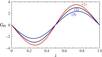
As for the linear problem, equation (5.2) with the boundary conditions (5.3) is solved numerically using a spectral Chebyshev collocation method. Figure 5 shows the modification of the conductive temperature profile at order
 $A^{2}$
for three values of
 $L_{s}$
. The warm upflow and cold downflow fluid tend to reduce the vertical temperature gradient of the basic state. For
 $L_{s}\rightarrow \infty$
, the numerical results are in very good quantitative agreement with the analytical solution
 $$\begin{eqnarray}G_{02}(z)=-\frac{3{\rm\pi}}{4}\sin (2{\rm\pi}z)\quad \text{for SFBC}.\end{eqnarray}$$
Modification of the conductive temperature profile at the critical conditions for
 $\mathit{Pr}=10$
and different values of
 $L_{s}$
: (1)
 $L_{s}=0$
NSBC; (2)
 $L_{s}=0.1$
; and (3)
 $L_{s}=10^{4}$
very close to SFBC.

5.2. First harmonic of the fundamental
A first harmonic term
 $\sum _{p=1}^{N}A_{p}^{2}F_{22}(z)E^{2\boldsymbol{k}_{p}\boldsymbol{\cdot }\boldsymbol{r}}$
is also produced by the interaction of the fundamental (4.1) with itself, through the quadratic nonlinear terms of the perturbations (2.17). Equations for
 $F_{22}$
and
 $G_{22}$
are obtained by setting
 $n=2,m=0$
in (4.18) and (4.19) and extracting the factor of
 $A_{p}^{2}E^{2\boldsymbol{k}_{p}\boldsymbol{\cdot }\boldsymbol{r}}$
in the nonlinear terms. We obtain
 $$\begin{eqnarray}\displaystyle & \left[\mathscr{S}_{2}^{2}-2(s/\mathit{Pr})\mathscr{S}_{2}\right]F_{22}-4k_{c}^{2}\mathit{Ra}G_{22}=(2/\mathit{Pr})\left(F_{11}D^{3}F_{11}-DF_{11}D^{2}F_{11}\right)\!, & \displaystyle\end{eqnarray}$$
 $$\begin{eqnarray}\displaystyle & F_{22}+\left(\mathscr{S}_{2}-2s\right)G_{22}=F_{11}\left(DG_{11}\right)-G_{11}\left(DF_{11}\right)\!. & \displaystyle\end{eqnarray}$$
 $F_{22}$
and
 $G_{22}$
are identical to those on
 $F_{11}$
and
 $G_{11}$
, (3.7a
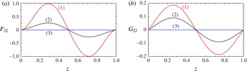
). The results are shown in figure 6. For SFBCs, we have
 $$\begin{eqnarray}F_{22}=G_{22}=0\end{eqnarray}$$
in agreement with the numerical results obtained at large
 $L_{s}$
.
First harmonic of the fundamental at the critical conditions for
 $\mathit{Pr}=10$
and different values of
 $L_{s}$
: (1)
 $L_{s}=0$
NSBC; (2)
 $L_{s}=0.1$
; and (3)
 $L_{s}=10^{4}$
very close to SFBC.

5.3. Quadratic interaction between Fourier modes with different wavevectors
The quadratic interaction of the fundamental mode with itself generates the first harmonic mode described in the above section, but also modes resulting from the interaction between modes with wavevectors
 $\boldsymbol{k}_{p}$
and
 $\boldsymbol{k}_{q}$
(
 $p\neq q$
). In the present study, the wavevectors lie on either a square or hexagonal lattice in the wavevector plane.
5.3.1. Square lattice
With
 $\boldsymbol{k}_{1}=k_{c}\boldsymbol{e}_{x}$
and
 $\boldsymbol{k}_{2}=k_{c}\boldsymbol{e}_{y}$
, modes generated at order
 $A_{1}A_{2}$
are
 $$\begin{eqnarray}A_{1}A_{2}\left[\begin{array}{@{}c@{}}F_{A_{1}A_{2}}(z)\\ G_{A_{1}A_{2}}(z)\end{array}\right]\exp \left[\text{i}(\boldsymbol{k}_{1}+\boldsymbol{k}_{2})\boldsymbol{\cdot }\boldsymbol{r}\right]+\text{c.c.},\end{eqnarray}$$
and
 $$\begin{eqnarray}A_{1}A_{2}\left[\begin{array}{@{}c@{}}\bar{F}_{A_{1}A_{2}}(z)\\ \bar{G}_{A_{1}A_{2}}(z)\end{array}\right]\exp \left[\text{i}(\boldsymbol{k}_{1}-\boldsymbol{k}_{2})\boldsymbol{\cdot }\boldsymbol{r}\right]+\text{c.c.}\end{eqnarray}$$
Since
 $F_{11}$
and
 $G_{11}$
are real,
 $(F_{A_{1}A_{2}},G_{A_{1}A_{2}})$
and
 $(\bar{F}_{A_{1}A_{2}},\bar{G}_{A_{1}A_{2}})$
are identical and real. They satisfy
 $$\begin{eqnarray}\displaystyle & & \displaystyle [(D^{2}-2k_{c}^{2})^{2}-2(s/\mathit{Pr})(D^{2}-2k_{c}^{2})]F_{A_{1}A_{2}}-2k_{c}^{2}\mathit{Ra}G_{A_{1}A_{2}}\nonumber\\ \displaystyle & & \displaystyle \quad =(2/\mathit{Pr})[F_{11}(D^{3}F_{11})+(DF_{11})(D^{2}F_{11})]-(4/\mathit{Pr})k_{c}^{2}F_{11}(DF_{11}],\end{eqnarray}$$
 $$\begin{eqnarray}(D^{2}-2k_{c}^{2}-2s)G_{A_{1}A_{2}}+F_{A_{1}A_{2}}=2F_{11}(DG_{11}).\end{eqnarray}$$
Boundary conditions on
 $(F_{A_{1}A_{2}},G_{A_{1}A_{2}})$
are the same as those on
 $(F_{11},G_{11})$
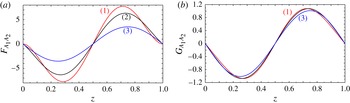
. The functions
 $F_{A_{1}A_{2}}$
and
 $G_{A_{1}A_{2}}$
are shown in figure 7 for different values of
 $L_{s}$
. The coupling between the modes
 $\exp (\text{i}k_{c}x)$
and
 $\exp (\text{i}k_{c}y)$
is significant and it is more important in the situation of wall adhesion than for SFBCs. In this latter case, at the critical conditions,
 $$\begin{eqnarray}\displaystyle & \displaystyle F_{A_{1}A_{2}}(z)=-\frac{27}{100}{\rm\pi}^{2}\left(\frac{{\rm\pi}}{\mathit{Pr}}+1\right)\sin (2{\rm\pi}z), & \displaystyle\end{eqnarray}$$
 $$\begin{eqnarray}\displaystyle & \displaystyle G_{A_{1}A_{2}}=-{\rm\pi}\frac{27+150\mathit{Pr}}{473\mathit{Pr}}\sin (2{\rm\pi}z). & \displaystyle\end{eqnarray}$$
 $A_{1}A_{2}$
, the nonlinear inertial terms in (2.16) cancel, and the vertical vorticity
 ${\it\zeta}$
obeys a diffusion equation: it thus can be ignored.
Modes generated in a square lattice at order
 $A_{1}A_{2}$
, at the critical conditions, for
 $\mathit{Pr}=10$
, and different values of
 $L_{s}$
: (1)
 $L_{s}=0$
(NSBC); (2)
 $L_{s}=0.1$
; and (3)
 $L_{s}=10^{4}$
very close to SFBC.

5.3.2. Hexagonal lattice
With
 $\boldsymbol{k}_{1}=k_{c}\boldsymbol{e}_{x},\boldsymbol{k}_{2}=k_{c}(-\boldsymbol{e}_{x}/2+(\sqrt{3}/2)\boldsymbol{e}_{y})$
and
 $\boldsymbol{k}_{3}=k_{c}(-\boldsymbol{e}_{x}/2-(\sqrt{3}/2)\boldsymbol{e}_{y})$
, modes generated at order
 $A_{p}A_{q}$
with
 $1\leqslant p\leqslant 3,~1\leqslant q\leqslant 3$
and
 $p\neq q$
are
 $$\begin{eqnarray}A_{p}A_{q}\left[\begin{array}{@{}c@{}}F_{A_{p}A_{q}}(z)\\ G_{A_{p}A_{q}}(z)\end{array}\right]\exp \left[\text{i}(\boldsymbol{k}_{p}+\boldsymbol{k}_{q})\boldsymbol{\cdot }\boldsymbol{r}\right]+\text{c.c.},\end{eqnarray}$$
and
 $$\begin{eqnarray}A_{p}A_{q}\left[\begin{array}{@{}c@{}}\bar{F}_{A_{p}A_{q}}(z)\\ \bar{G}_{A_{p}A_{q}}(z)\end{array}\right]\exp \left[\text{i}(\boldsymbol{k}_{p}-\boldsymbol{k}_{q})\boldsymbol{\cdot }\boldsymbol{r}\right]+\text{c.c.}\end{eqnarray}$$
The functions
 $F_{ApAq}$
and
 $G_{ApAq}$
satisfy
 $$\begin{eqnarray}\displaystyle & & \displaystyle [(D^{2}-k_{c}^{2})^{2}-2(s/\mathit{Pr})(D^{2}-k_{c}^{2})]F_{A_{p}A_{q}}-k_{c}^{2}\mathit{Ra}G_{A_{p}A_{q}}\nonumber\\ \displaystyle & & \displaystyle \quad =(1/\mathit{Pr})\left[F_{11}D^{3}F_{11}+2\left(DF_{11}\right)\left(D^{2}F_{11}\right)-3k_{c}^{2}F_{11}\left(DF_{11}\right)\right]\!,\end{eqnarray}$$
 $$\begin{eqnarray}\displaystyle & & \displaystyle \left(D^{2}-k_{c}^{2}-2s\right)G_{A_{p}A_{q}}+F_{A_{p}A_{q}}=2F_{11}\left(DG_{11}\right)+G_{11}\left(DF_{11}\right)\!.\end{eqnarray}$$
 $\bar{F}_{ApAq}$
and
 $\bar{G}_{ApAq}$
satisfy
 $$\begin{eqnarray}\displaystyle & & \displaystyle [(D^{2}-3k_{c}^{2})^{2}-(2s/\mathit{Pr})(D^{2}-3k_{c}^{2})]\bar{F}_{A_{p}A_{q}}-3k_{c}^{2}\mathit{Ra}\bar{G}_{A_{p}A_{q}}\nonumber\\ \displaystyle & & \displaystyle \quad =(3/\mathit{Pr})\left[F_{11}\left(D^{3}F_{11}\right)-k_{c}^{2}F_{11}\left(DF_{11}\right)\right]\!,\end{eqnarray}$$
 $$\begin{eqnarray}\displaystyle & & \displaystyle \left(D^{2}-3k_{c}^{2}-2s\right)\bar{G}_{A_{p}A_{q}}+\bar{F}_{A_{p}A_{q}}=2F_{11}\left(DG_{11}\right)-G_{11}\left(DF_{11}\right)\!.\end{eqnarray}$$
 $(F_{A_{p}A_{q}},G_{A_{p}A_{q}})$
and
 $(\bar{F}_{A_{p}A_{q}},\bar{G}_{A_{p}A_{q}})$
are the same as the ones on
 $(F_{11},G_{11})$
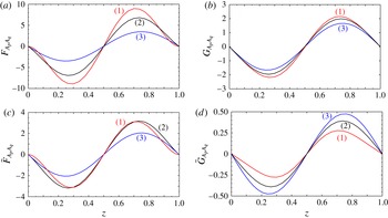
. In figure 8, the functions
 $F_{A_{p}Aq},G_{ApAq},\bar{F}_{ApAq}$
and
 $\bar{G}_{ApA_{q}}$
are plotted at the critical conditions,
 $\mathit{Pr}=10$
and different values of the slip parameter. For SFBCs, at the critical conditions,
 $$\begin{eqnarray}F_{A_{p}A_{q}}=-\frac{9{\rm\pi}^{3}}{104}\left(1+\frac{3}{\mathit{Pr}}\right)\sin (2{\rm\pi}z),\quad G_{A_{p}A_{q}}=-\frac{3{\rm\pi}}{52}\left(9+\frac{1}{\mathit{Pr}}\right)\sin (2{\rm\pi}z),\end{eqnarray}$$
 $$\begin{eqnarray}\bar{F}_{A_{p}A_{q}}=-\frac{81{\rm\pi}^{3}}{5000}\left(3+\frac{11}{\mathit{Pr}}\right)\sin (2{\rm\pi}z),\quad \bar{G}_{A_{p}A_{q}}=-\frac{3{\rm\pi}}{2500}\left(121+\frac{27}{\mathit{Pr}}\right)\sin (2{\rm\pi}z).\end{eqnarray}$$
As for squares, the amplitude of modes arising from the quadratic coupling between modes with vector
 $\boldsymbol{k}_{p}$
and
 $\boldsymbol{k}_{q}$
is more important than that of the first harmonic.
Modes generated in an hexagonal lattice at the critical conditions for
 $\mathit{Pr}=10$
: factor of
 $A_{p}A_{q}\exp [\text{i}(\boldsymbol{k}_{p}+\boldsymbol{k}_{q})\boldsymbol{\cdot }\boldsymbol{r}]$
in (a,b) and
 $A_{p}A_{q}\exp [\text{i}(\boldsymbol{k}_{p}-\boldsymbol{k}_{q})\boldsymbol{\cdot }\boldsymbol{r}]$
in (c,d), with (1)
 $L_{s}=0$
, (2)
 $L_{s}=0.1$
and (3)
 $L_{s}=10^{4}$
.

5.4. Modification of the fundamental at cubic order: nature of the bifurcation
The nonlinear interactions between the fundamental, its first harmonic, the modification of the conductive temperature profile and modes generated through different couplings, lead to a cubic correction
 $O(A_{p}^{3})$
to the fundamental mode. The first Landau coefficient accounts for the feedback of these nonlinear interactions on the fundamental mode. It is determined for the three convective patterns and the nature of the bifurcation is deduced.
The nonlinearity of the rheological law intervenes through the term
 $({\it\mu}-1)\dot{{\bf\gamma}}$
in (2.16) and (2.17). At cubic order, because of (2.10), it reduces to
 $$\begin{eqnarray}({\it\mu}-1)\dot{{\bf\gamma}}=-{\it\alpha}{\it\Gamma}\dot{{\bf\gamma}}.\end{eqnarray}$$
5.4.1. Bifurcation to rolls
The modification of the fundamental at order
 $A^{3}$
is governed by (4.18) and (4.19) with
 $m=n=1$
, i.e.
 $$\begin{eqnarray}\displaystyle & \displaystyle \left(\mathscr{S}_{1}^{2}-3\frac{s}{\mathit{Pr}}\mathscr{S}_{1}\right)F_{13}-k_{c}^{2}\mathit{Ra}G_{13}=\frac{g_{1}}{\mathit{Pr}}\mathscr{S}_{1}F_{11}-\left[NI_{w}\right]_{E^{1}A^{3}}-\left[NV\right]_{E^{1}A^{3}}\!, & \displaystyle\end{eqnarray}$$
 $$\begin{eqnarray}\displaystyle & \left(\mathscr{S}_{1}-3s\right)G_{13}+F_{13}=g_{1}G_{11}-\left[NI_{{\it\theta}}\right]_{E^{1}A^{3}}\!. & \displaystyle\end{eqnarray}$$
 $$\begin{eqnarray}\displaystyle & \displaystyle F_{13}=0,\quad DF_{13}-L_{s}D^{2}F_{13}={\it\alpha}L_{s}\frac{\partial }{\partial x}\left({\it\Gamma}\frac{\partial u}{\partial z}\right)_{E^{1}A^{3}}\!,\quad G_{13}=0\quad \text{at}~z=0, & \displaystyle\end{eqnarray}$$
 $$\begin{eqnarray}\displaystyle & \displaystyle F_{13}=0,\quad DF_{13}+L_{s}D^{2}F_{13}=-{\it\alpha}L_{s}\frac{\partial }{\partial x}\left({\it\Gamma}\frac{\partial u}{\partial z}\right)_{E^{1}A^{3}}\!,\quad G_{13}=0\quad \text{at}~z=1.~\ & \displaystyle\end{eqnarray}$$
 $$\begin{eqnarray}\displaystyle & F_{13}=DF_{13}=0\quad \text{at}~z=0,1~\text{for NSBC}, & \displaystyle\end{eqnarray}$$
 $$\begin{eqnarray}\displaystyle & \displaystyle F_{13}=D^{2}F_{13}=0\quad \text{at}~z=0,1~\text{for SFBC}. & \displaystyle\end{eqnarray}$$
 $$\begin{eqnarray}\boldsymbol{L}\boldsymbol{\cdot }\boldsymbol{X}_{13}=g_{1}\boldsymbol{M}\boldsymbol{\cdot }\boldsymbol{X}_{11}-\boldsymbol{NI}-\boldsymbol{NV}+3s\boldsymbol{M}\boldsymbol{\cdot }\boldsymbol{X}_{13}\quad \text{with}~\boldsymbol{X}_{13}=\left(F_{13},G_{13}\right)\!.\end{eqnarray}$$
The nature of the bifurcation is determined at the critical conditions, i.e.
 $s=0$
.
In order to calculate the first Landau coefficient
 $g_{1}$
from the Fredholm solvability condition, i.e. orthogonality of the inhomogeneous part of (5.28) to the null-space of the adjoint operator of
 $\boldsymbol{L}$
, we decompose
 $\boldsymbol{X}_{13}$
into a homogeneous
 $\boldsymbol{X}_{13H}$
and inhomogeneous
 $\boldsymbol{X}_{13NH}$
parts:
 $$\begin{eqnarray}\boldsymbol{X}_{13}=\boldsymbol{X}_{13H}+\boldsymbol{X}_{13NH}.\end{eqnarray}$$
Here
 $\boldsymbol{X}_{13H}$
satisfies
 $$\begin{eqnarray}\boldsymbol{L}\boldsymbol{\cdot }\boldsymbol{X}_{13H}=g_{1H}\boldsymbol{M}\boldsymbol{\cdot }\boldsymbol{X}_{11}-\boldsymbol{N}\boldsymbol{I}-\boldsymbol{N}\boldsymbol{V},\end{eqnarray}$$
with homogeneous boundary conditions, i.e.
 $F_{13H}=DF_{13H}-L_{s}D^{2}F_{13H}=0$
at
 $z=0$
and similarly at
 $z=1$
. By applying the solvability condition to (5.30), we obtain
 $$\begin{eqnarray}g_{1H}=\langle \boldsymbol{NI}+\boldsymbol{NV},\tilde{\boldsymbol{X}}_{ad}\rangle ,\quad \tilde{\boldsymbol{X}}_{ad}=\frac{\boldsymbol{X}_{ad}}{\left\langle \boldsymbol{M}\boldsymbol{\cdot }\boldsymbol{X}_{11},\boldsymbol{X}_{ad}\right\rangle }.\end{eqnarray}$$
Then
 $\boldsymbol{X}_{13H}$
is then determined by solving (5.30). Here,
 $\boldsymbol{X}_{13NH}$
is a correction term that accounts for the non-homogeneity of the boundary conditions. Substituting (5.29) into (5.28), we obtain at the critical conditions
 $$\begin{eqnarray}\boldsymbol{L}\boldsymbol{\cdot }\boldsymbol{X}_{13H}=g_{1}\boldsymbol{M}\boldsymbol{\cdot }\boldsymbol{X}_{11}-\boldsymbol{NI}-\boldsymbol{NV}-\boldsymbol{L}\boldsymbol{\cdot }\boldsymbol{X}_{13NH}.\end{eqnarray}$$
By applying the solvability condition to (5.32), we get
 $$\begin{eqnarray}g_{1}=g_{1H}+\langle \boldsymbol{L}\boldsymbol{\cdot }\boldsymbol{X}_{13NH},\tilde{\boldsymbol{X}}_{ad}\rangle .\end{eqnarray}$$
The technique of solution adopted is to iterate a few times between (5.28) and (5.33). At the start,
 $\boldsymbol{X}_{13NH}$
is assumed to be identically zero in (5.33). A first approximation to
 $g_{1}$
is then obtained:
 $g_{1}^{(1)}=g_{1H}$
. This is put into (5.28), which is solved at the critical conditions, with non-homogeneous boundary conditions, to obtain a first approximation of
 $\boldsymbol{X}_{13}$
. Using (5.29), a first approximation of
 $\boldsymbol{X}_{13NH}$
is deduced. Then
 $\boldsymbol{X}_{13NH}$
is put into (5.33). This process is repeated until it converges to a desired level of accuracy. Note that (5.28) and (5.30) are solved with an additional condition
 $$\begin{eqnarray}\boldsymbol{X}_{13}=\boldsymbol{X}_{13H}=0\quad \text{at}~z=1/2,\end{eqnarray}$$
as suggested by Herbert (Reference Herbert1980, Reference Herbert1983), Sen & Venkateswarlu (Reference Sen and Venkateswarlu1983) and Generalis & Fujimura (Reference Generalis and Fujimura2009). Without this normalization,
 $\boldsymbol{X}_{13}$
is defined up to an arbitrary multiple of the solution
 $\boldsymbol{X}_{11}$
of the linear problem (3.8). Finally,
 $g_{1}$
can be written as the sum of three contributions. The first one arises from the nonlinear inertial terms
 $\boldsymbol{NI}$
, the second from the nonlinear viscous terms
 $\boldsymbol{NV}$
and the third from the inhomogeneity of the boundary conditions,
 $$\begin{eqnarray}g_{1}=g_{1}^{I}+g_{1}^{V}+g_{1}^{NH}\end{eqnarray}$$
with
 $$\begin{eqnarray}g_{1}^{I}=\langle \boldsymbol{NI},\tilde{\boldsymbol{X}}_{ad}\rangle ,\quad g_{1}^{V}=\langle \boldsymbol{NV},\tilde{\boldsymbol{X}}_{ad}\rangle ,\quad g_{1}^{NH}=\langle \boldsymbol{L}\boldsymbol{\cdot }\boldsymbol{X}_{13NH},\tilde{\boldsymbol{X}}_{ad}\rangle .\end{eqnarray}$$
Using (5.22), the contribution of the nonlinear viscous term
 $g_{1}^{V}$
can be written as
 $$\begin{eqnarray}g_{1}^{V}=-{\it\alpha}g_{1}^{NN},\end{eqnarray}$$
with
 ${\it\alpha}$
defined by (2.11) and
 $g_{1}^{NN}$
that does not depend on the rheological parameters. Similarly, it can be shown that
 $X_{13NH}=-{\it\alpha}\tilde{X}_{13NH}$
, where
 $\tilde{X}_{13NH}$
does not depend on the rheological parameters. Hence,
 $$\begin{eqnarray}g_{1}^{NH}=-{\it\alpha}g_{1}^{BC}\quad \text{with}~g_{1}^{BC}=\langle \boldsymbol{L}\boldsymbol{\cdot }\tilde{\boldsymbol{X}}_{13NH},\tilde{\boldsymbol{X}}_{ad}\rangle .\end{eqnarray}$$
Note that, for NSBCs and SFBCs,
 $$\begin{eqnarray}\boldsymbol{X}_{13NH}=0\quad \text{thus}~g_{1}^{BC}=0.\end{eqnarray}$$
The first Landau constant
 $g_{1}$
as well as the different contributions
 $g_{1}^{I},g_{1}^{V}$
and
 $g_{1}^{NH}$
are determined for different critical sets
 $(\mathit{Ra}_{c},k_{c},L_{s},\mathit{Pr})$
and different values of the degree of shear-thinning
 ${\it\alpha}$
. The integrals in (5.36) are evaluated numerically by means of Clenshaw and Curtis method.
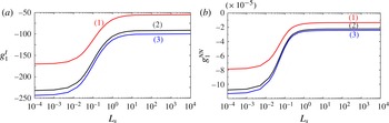
In figure 9(a),
 $g_{1}^{I}$
is plotted as a function of
 $L_{s}$
. As expected,
 $g_{1}^{I}$
is negative, i.e. the bifurcation is supercritical for a Newtonian fluid. The absolute value of
 $g_{1}^{I}$
decreases with increasing
 $L_{s}$
, i.e. slip promotes the development of the convection. For SFBCs, an analytical expression of
 $g_{1}^{I}$
is obtained,
 $$\begin{eqnarray}g_{1}^{I}=-\frac{9{\rm\pi}^{4}}{8}\frac{\mathit{Pr}}{1+\mathit{Pr}}.\end{eqnarray}$$
The contribution of the nonlinear inertial terms gathers the feedback from thermal advection terms and velocity terms:
 $$\begin{eqnarray}\displaystyle g_{1}^{I} & = & \displaystyle \langle NI_{w}(F_{22}|F_{11}),\tilde{F}_{ad}\rangle +\langle NI_{{\it\theta}}(G_{22}|F_{11}),\tilde{G}_{ad}\rangle \nonumber\\ \displaystyle & & \displaystyle +\,\langle NI_{{\it\theta}}(F_{22}|G_{11}),\tilde{G}_{ad}\rangle +\langle NI_{{\it\theta}}(G_{02}|F_{11}),\tilde{G}_{ad}\rangle .\end{eqnarray}$$
For
 $\mathit{Pr}\geqslant 1$
, the analysis of the different terms shows that
 $g_{1}^{I}$
is dominated by the nonlinear thermal convection terms, more precisely the term involving
 $G_{02}$
, the modification of the conductive temperature. The contributions of the other nonlinear inertial term is practically negligible.
Contribution of the nonlinear inertial terms (a) and nonlinear viscous terms (b) to the first cubic Landau constant, versus the slip parameter
 $L_{s}$
for different values of the Prandtl number: (1)
 $\mathit{Pr}=1$
, (2)
 $\mathit{Pr}=5$
, (3)
 $\mathit{Pr}=10$
.

In figure 9(b), we plot
 $g_{1}^{NN}$
as a function of
 $L_{s}$
for different values of
 $\mathit{Pr}$
. For SFBCs, an analytical expression is obtained,
 $$\begin{eqnarray}g_{1}^{NN}=-\frac{1803{\rm\pi}^{8}}{64}\frac{\mathit{Pr}}{1+\mathit{Pr}}.\end{eqnarray}$$
As can be observed,
 $g_{1}^{NN}$
is negative, and
 $g_{1}^{V}=-{\it\alpha}g_{1}^{NN}>0$
. Therefore, shear-thinning effects promote a subcritical bifurcation, which is understandable since the viscosity, which damps convection, is reduced.
Concerning
 $g_{1}^{NH}$
, its absolute value does not exceed
 $g_{1}/100$
. The maximum value is reached at
 $L_{s}\approx 0.1$
.
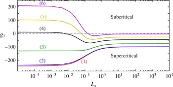
In figure 10 we plot
 $g_{1}$
as a function of
 $L_{s}$
at
 $\mathit{Pr}=10$
and different values of
 ${\it\alpha}$
. For low shear-thinning effects,
 $g_{1}<0$
and the bifurcation is supercritical, while for sufficiently high shear-thinning effects,
 $g_{1}>0$
and the bifurcation is subcritical. Using (5.35) and (5.37), the critical degree of shear-thinning
 ${\it\alpha}_{c}$
above which the bifurcation changes from supercritical to subcritical is given by
 $$\begin{eqnarray}{\it\alpha}_{c}=\frac{g_{1}^{I}}{g_{1}^{NN}+g_{1}^{BC}}.\end{eqnarray}$$
Cubic Landau constant versus
 $L_{s}$
at
 $\mathit{Pr}=10$
and different values of
 ${\it\alpha}$
: (1)
 ${\it\alpha}=0$
, i.e. Newtonian case; (2)
 ${\it\alpha}=6.25\times 10^{-6}$
; (3)
 ${\it\alpha}=10^{-4}$
; (4)
 ${\it\alpha}=2.25\times 10^{-4}$
; (5)
 ${\it\alpha}=3.0625\times 10^{-4}$
; (6)
 ${\it\alpha}=4\times 10^{-4}$
.

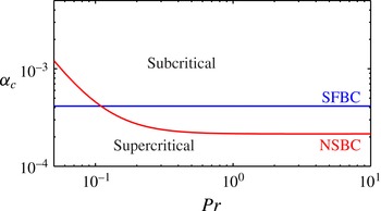
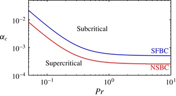
Figure 11 shows the variation of
 ${\it\alpha}_{c}$
as a function of
 $\mathit{Pr}$
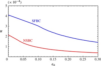
for NSBCs and SFBCs. For this latter case, we have
 $$\begin{eqnarray}{\it\alpha}_{c}=\frac{24}{601{\rm\pi}^{4}}\approx 4.1\times 10^{-4}.\end{eqnarray}$$
This result agrees with Balmforth & Rust (Reference Balmforth and Rust2009) but disagrees with the value
 ${\it\alpha}_{c}=14\times 10^{-4}$
found by Albaalbaki & Khayat (Reference Albaalbaki and Khayat2011). For NSBCs, and
 $\mathit{Pr}\geqslant 1$
,
 ${\it\alpha}_{c}=2.15\times 10^{-4}$
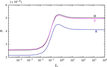
. The plot of
 ${\it\alpha}_{c}$
versus
 $L_{s}$
for
 $\mathit{Pr}=10$
is visible in figure 14, which also displays some results for two other patterns.
Critical value of the degree of shear-thinning
 ${\it\alpha}_{c}$
above which the bifurcation to rolls becomes subcritical, versus Prandtl number.

5.4.2. Bifurcation to squares
As compared with rolls, for square patterns, the modification of the fundamental comprises an additional term, which arises from the interaction of modes with wavevectors
 $\boldsymbol{k}_{1}=k_{c}\boldsymbol{e}_{x}$
and
 $\boldsymbol{k}_{2}=k_{c}\boldsymbol{e}_{y}$
. Hence, the modification of the fundamental
 $$\begin{eqnarray}w=F_{13}(z)\left(A_{1}^{3}\text{e}^{\text{i}k_{c}x}+A_{2}^{3}\text{e}^{\text{i}k_{c}y}+\text{c.c.}\right)+\tilde{F}_{13}(z)\left(A_{2}^{2}A_{1}\text{e}^{\text{i}k_{c}x}+A_{1}^{2}A_{2}\text{e}^{\text{i}k_{c}y}+\text{c.c.}\right)\!,\end{eqnarray}$$
and similarly for
 ${\it\theta}$
by replacing
 $F$
by
 $G$
. The amplitude equations for
 $A_{1}$
and
 $A_{2}$
are obtained using symmetries introduced by the square lattice. Employing crystallographic terminology (Golubitsky et al.
Reference Golubitsky, Swift and Knoblock1984; McKenzie Reference McKenzie1988; Silber & Knoblock Reference Silber and Knoblock1988), these are the symmetries of a square
 $D_{4}$
in addition to the two-torus
 $T_{2}$
of translation in the two horizontal directions. Requiring equivariance with respect to the group
 $D_{4}\times T_{2}$
leads to the amplitude equations
 $$\begin{eqnarray}\displaystyle & \displaystyle \frac{\text{d}A_{1}}{\text{d}t}=sA_{1}+\left(g_{1}A_{1}^{2}+{\it\lambda}_{1}A_{2}^{2}\right)A_{1}, & \displaystyle\end{eqnarray}$$
 $$\begin{eqnarray}\displaystyle & \displaystyle \frac{\text{d}A_{2}}{\text{d}t}=sA_{2}+\left(g_{1}A_{2}^{2}+{\it\lambda}_{1}A_{1}^{2}\right)A_{2}. & \displaystyle\end{eqnarray}$$
 $g_{1}$
and the coupling coefficient
 ${\it\lambda}_{1}$
are real.
Equations satisfied by
 $\tilde{F}_{13}(z)$
and
 $\tilde{G}_{13}(z)$
are similar to that satisfied by
 $F_{13}(z)$
and
 $G_{13}(z)$
, i.e. (5.23) and (5.24), respectively, by replacing
 $g_{1}$
by
 ${\it\lambda}_{1}$
and evaluating the nonlinear forcing terms that are factor of
 $A_{2}^{2}A_{1}\exp (\text{i}k_{c}x)$
. At criticality,
 $s=0$
, the coupling coefficient
 ${\it\lambda}_{1}$
is obtained with a solvability condition. As for
 $g_{1}$
, it can be written
 $$\begin{eqnarray}{\it\lambda}_{1}={\it\lambda}_{1}^{I}-{\it\alpha}{\it\lambda}_{1}^{NN}-{\it\alpha}{\it\lambda}_{1}^{BC}.\end{eqnarray}$$
For SFBCs,
 $$\begin{eqnarray}{\it\lambda}_{1}^{I}=-\frac{9{\rm\pi}^{4}\left(120+72\mathit{Pr}+673\mathit{Pr}^{2}\right)}{3784\mathit{Pr}\left(1+\mathit{Pr}\right)},\quad {\it\lambda}_{1}^{NN}=-\frac{921{\rm\pi}^{8}\mathit{Pr}}{32(1+\mathit{Pr})},\quad {\it\lambda}_{1}^{BC}=0.\end{eqnarray}$$
The critical value of
 ${\it\alpha}$
above which the bifurcation to squares becomes subcritical,
 $$\begin{eqnarray}{\it\alpha}_{c}=\frac{g_{1}^{I}+{\it\lambda}_{1}^{I}}{\left(g_{1}^{NN}+{\it\lambda}_{1}^{NN}\right)+\left(g_{1}^{BC}+{\it\lambda}_{1}^{BC}\right)}.\end{eqnarray}$$
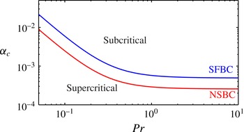
Figure 12 shows the variation of
 ${\it\alpha}_{c}$
as a function of
 $\mathit{Pr}$
for NSBC and SFBC. In this latter case,
 $$\begin{eqnarray}{\it\alpha}_{c}=\frac{16\left(20+12\mathit{Pr}+191\mathit{Pr}^{2}\right)}{63\,855{\rm\pi}^{4}\mathit{Pr}^{2}}.\end{eqnarray}$$
Critical value of the degree of shear-thinning
 ${\it\alpha}_{c}$
above which the bifurcation to squares becomes subcritical, versus Prandtl number.

5.4.3. Bifurcation to hexagons
For hexagonal patterns, the modification of the fundamental modes reads
 $$\begin{eqnarray}\displaystyle w & = & \displaystyle F_{13}(z)\left(A_{1}^{3}\text{e}^{\text{i}\boldsymbol{k}_{1}\boldsymbol{\cdot }\boldsymbol{r}}+A_{2}^{3}\text{e}^{\text{i}\boldsymbol{k}_{2}\boldsymbol{\cdot }\boldsymbol{r}}+A_{3}^{3}\text{e}^{\text{i}\boldsymbol{k}_{3}\boldsymbol{\cdot }\boldsymbol{r}}+\text{c.c.}\right)+\tilde{\tilde{F}}_{13}(z)\left[\left(A_{2}^{2}+A_{3}^{2}\right)A_{1}\text{e}^{\text{i}\boldsymbol{k}_{1}\boldsymbol{\cdot }\boldsymbol{r}}\right.\nonumber\\ \displaystyle & & \displaystyle +\,\left.\left(A_{3}^{2}+A_{1}^{2}\right)A_{2}\text{e}^{\text{i}\boldsymbol{k}_{2}\boldsymbol{\cdot }\boldsymbol{r}}+\left(A_{1}^{2}+A_{2}^{2}\right)A_{3}\text{e}^{\text{i}\boldsymbol{k}_{3}\boldsymbol{\cdot }\boldsymbol{r}}+\text{c.c.}\right]\!,\end{eqnarray}$$
and similarly for
 ${\it\theta}$
by replacing
 $F$
by
 $G$
. The amplitude equations for
 $A_{1},A_{2}$
and
 $A_{3}$
are obtained using symmetries introduced by the hexagonal lattice. The symmetry group that leaves the hexagonal lattice invariant is
 $D_{6}\times T_{2}$
;
 $D_{6}$
represents the rotational (
 $2{\rm\pi}/3$
) and reflection symmetries. The amplitude equations are (Golubitsky et al.
Reference Golubitsky, Swift and Knoblock1984)
 $$\begin{eqnarray}\frac{\text{d}A_{1}}{\text{d}t}=sA_{1}+\left[g_{1}A_{1}^{2}+{\it\delta}_{1}\left(A_{2}^{2}+A_{3}^{2}\right)\right]A_{1}.\end{eqnarray}$$
Equations for
 $\text{d}A_{2}/\text{d}t,~\text{d}A_{3}/\text{d}t$
are obtained by cyclic permutation of
 $A_{1},A_{2}$
and
 $A_{3}$
. The quadratic term proportional to
 $A_{2}A_{3}$
in (5.53) is equivariant with respect to the group
 $D_{6}\times T_{2}$
, but vanishes here because of the up and down reflection symmetry. Equations satisfied by
 $\tilde{\tilde{F}}_{13}(z)$
and
 $\tilde{\tilde{G}}_{13}(z)$
are similar to that satisfied by
 $F_{13}(z)$
and
 $G_{13}(z)$
, i.e. (5.23) and (5.24), respectively, by replacing
 $g_{1}$
by
 ${\it\delta}_{1}$
and evaluating the nonlinear forcing terms that are factor of
 $A_{2}^{2}A_{1}\exp (\text{i}k_{c}x)$
. The determination of
 ${\it\delta}_{1}$
follows the same procedure as for
 $g_{1}$
and
 ${\it\lambda}_{1}$
. As previously, the coupling coefficient
 ${\it\delta}_{1}$
can be written
 $$\begin{eqnarray}{\it\delta}_{1}={\it\delta}_{1}^{I}-{\it\alpha}{\it\delta}_{1}^{NN}-{\it\alpha}{\it\delta}_{1}^{BC}.\end{eqnarray}$$
For SFBCs
 $$\begin{eqnarray}{\it\delta}_{1}^{I}=-\frac{9{\rm\pi}^{4}\left(1728+1113\mathit{Pr}+1273\mathit{Pr}^{2}\right)}{65\,000\mathit{Pr}\left(1+\mathit{Pr}\right)},\quad {\it\delta}_{1}^{NN}=-\frac{2175{\rm\pi}^{8}\mathit{Pr}}{64\left(1+\mathit{Pr}\right)},\quad {\it\delta}_{1}^{BC}=0.\end{eqnarray}$$
The critical value of the degree of shear-thinning
 ${\it\alpha}$
above which the bifurcation to hexagons becomes subcritical
 $$\begin{eqnarray}{\it\alpha}_{c}=\frac{g_{1}^{I}+2{\it\delta}_{1}^{I}}{\left(g_{1}^{NN}+2{\it\delta}_{1}^{NN}\right)+\left(g_{1}^{NH}+2{\it\delta}_{1}^{BC}\right)}.\end{eqnarray}$$
The variation of
 ${\it\alpha}_{c}$
as a function of
 $\mathit{Pr}$
is plotted in figure 13 for NSBC and SFBC. In this latter case,
 $$\begin{eqnarray}{\it\alpha}_{c}=\frac{24\left(3456+2226\mathit{Pr}+33\,599\mathit{Pr}^{2}\right)}{16\,664\,375{\rm\pi}^{4}\mathit{Pr}^{2}}.\end{eqnarray}$$
Finally, figure 14 shows
 ${\it\alpha}_{c}$
versus
 $L_{s}$
for rolls, squares and hexagons, at
 $\mathit{Pr}=10$
.
Critical value of the degree of shear-thinning
 ${\it\alpha}_{c}$
above which the bifurcation to hexagons becomes subcritical, versus Prandtl number.

For rolls (R), squares (S) and hexagons (H), critical value of the degree of shear-thinning
 ${\it\alpha}_{c}$
, versus the slip parameter
 $L_{s}$
for
 $\mathit{Pr}=10$
.

From now on, for the sake of simplicity, in order to not overload this article, we restrict ourselves to the two limiting cases
 $L_{s}=0$
, NSBCs, or
 $L_{s}=+\infty$
, SFBCs.
Remark. In this study, the midplane reflection symmetry is not broken (see appendix D). The amplitude equation at cubic order does not contain a quadratic term. Therefore, the bifurcation is of pitchfork type. It is either supercritical or subcritical depending on the sign of the cubic term. In the presence of non-Boussinesq effects, for instance, in fluids with thermodependent viscosity, the midplane reflection symmetry is broken and a quadratic term appears in the amplitude equation. In general, the presence of the quadratic term can lead to a bifurcation of transcritical type with a hexagonal planform.
5.5. Pattern selection
In this section, we investigate the competition between rolls and squares, and between rolls and hexagons, when we depart from the critical conditions. The calculation proceeds in two stages. First, the possible steady-state solutions of the amplitude equations are determined. Then, their linear stability is considered. However, this study requires the prior evaluation of the saturation and coupling coefficients in the amplitude equations, outside the critical conditions.
5.5.1. Saturation and coupling coefficients outside the critical conditions
Departing sufficiently from the critical conditions, we can no longer assume
 $s=0$
in the equations that describe the modification of the fundamental at cubic order. Hence, these equations become unconditionally solvable. To calculate
 $g_{1}$
,
 ${\it\lambda}_{1}$
or
 ${\it\delta}_{1}$
, an iterative process is used as suggested by Sen & Venkateswarlu (Reference Sen and Venkateswarlu1983). Details of the procedure are given in appendix B.
Figure 15 shows the variation of the ratios
 $g_{1}^{I}({\it\epsilon})/g_{1}^{I}({\it\epsilon}=0)$
and
 $g_{1}^{NN}({\it\epsilon})/g_{1}^{NN}({\it\epsilon}=0)$
versus the reduced Rayleigh number
 ${\it\epsilon}=\mathit{Ra}/\mathit{Ra}_{c}-1$
. The contribution to
 $g_{1}$
of the non-Newtonian viscous terms increases more rapidly than that of the inertial terms. At
 ${\it\epsilon}=0$
, the saturation coefficient
 $g_{1}=g_{1}^{I}-{\it\alpha}g_{1}^{NN}$
changes sign for
 ${\it\alpha}={\it\alpha}_{c}$
. It is clear from figure 15 that, for
 ${\it\epsilon}\neq 0$
,
 $g_{1}$
changes sign for
 ${\it\alpha}<{\it\alpha}_{c}$
. This result will be used when determining the domain of existence of the stationary solutions of the amplitude equations at cubic order.
For rolls, ratios
 $g_{1}^{I}/g_{1}^{I}~({\it\epsilon}=0)$
and
 $g_{1}^{NN}/g_{1}^{NN}~({\it\epsilon}=0)$
versus the reduced Rayleigh number,
 ${\it\epsilon}$
: (1)
 $g_{1}^{I}/g_{1}^{I}~({\it\epsilon}=0)$
for SFBC; (2)
 $g_{1}^{I}/g_{1}^{I}~({\it\epsilon}=0)$
for NSBC; (3)
 $g_{1}^{NN}/g_{1}^{NN}~({\it\epsilon}=0)$
for SFBC; and (4)
 $g_{1}^{NN}/g_{1}^{NN}~({\it\epsilon}=0)$
for NSBC.

Ratios between the coupling and saturation coefficients play a fundamental role in the pattern selection. They are shown in figure 16 versus the reduced Rayleigh number, for different values of
 ${\it\alpha}$
,
 $\mathit{Pr}=10$
and NSBCs; similar curves are obtained for SFBCs. For
 ${\it\alpha}\leqslant 0.9{\it\alpha}_{c}$
, one has: (i)
 ${\it\lambda}_{1},{\it\delta}_{1}$
and
 $g_{1}$
are of the same, negative, sign; (ii)
 $|{\it\lambda}_{1}|>|g_{1}|$
and
 $|{\it\delta}_{1}|>|g_{1}|$
; and (iii)
 ${\it\lambda}_{1}/g_{1}$
and
 ${\it\delta}_{1}/g_{1}$
increase with increasing shear-thinning effects.
For squares and hexagons, ratios (a)
 ${\it\lambda}_{1}/g_{1}$
and (b)
 ${\it\delta}_{1}/g_{1}$
versus the reduced Rayleigh number, at
 $\mathit{Pr}=10$
and different values of
 ${\it\alpha}$
in the case of NSBC: (1)
 ${\it\alpha}=0$
, Newtonian fluid; (2)
 ${\it\alpha}=0.1{\it\alpha}_{c}$
; (3)
 ${\it\alpha}=0.2{\it\alpha}_{c}$
; (4)
 ${\it\alpha}=0.3{\it\alpha}_{c}$
;(5)
 ${\it\alpha}=0.4{\it\alpha}_{c}$
; (6)
 ${\it\alpha}=0.5{\it\alpha}_{c}$
; (7)
 ${\it\alpha}=0.6{\it\alpha}_{c}$
; and (8)
 ${\it\alpha}=0.7{\it\alpha}_{c}$
.

5.5.2. Pattern selection on a square lattice
The amplitude equations satisfying the symmetry requirements of a square lattice are (5.46) and (5.47). The coefficients
 $s$
,
 $g_{1}$
and
 ${\it\lambda}_{1}$
in these equations depend on
 ${\it\alpha}$
and on the reduced Rayleigh number
 ${\it\epsilon}$
. The stationary solutions are obtained by setting
 $f_{i}(A_{1},A_{2})=0$
, where
 $f_{i}$
is the right-hand side of the amplitude equations. Their stability is determined by the sign of the eigenvalues
 ${\it\chi}_{i}$
of the Jacobian matrix
 $\unicode[STIX]{x1D611}_{ij}=\partial f_{i}/\partial A_{j}$
evaluated at steady states. In the following, the stability of the stationary solutions is examined in detail.
(i) Conduction state,
 $A_{1}=A_{2}=0$
. The stability eigenvalues associated to this state are
 ${\it\chi}_{1}={\it\chi}_{2}=s$
. The conductive state is stable if
 ${\it\epsilon}<0$
and unstable if
 ${\it\epsilon}>0$
.
(ii) Steady convection with rolls,
 $A_{1}=\sqrt{-s/g_{1}},A_{2}=0$
or
 $A_{1}=0,A_{2}=\sqrt{-s/g_{1}}$
. The associated eigenvalues are:
 ${\it\chi}_{1}=-2s$
and
 ${\it\chi}_{2}=s((g_{1}-{\it\lambda}_{1})/g_{1})$
. In the supercritical regime, according to figures 10 and 16(a),
 $g_{1}$
and
 ${\it\lambda}_{1}$
are negative and
 $|{\it\lambda}_{1}|>|g_{1}|$
. Thus, stable rolls appear at a supercritical bifurcation from
 ${\it\epsilon}=0$
. In the neighbourhood of the points (
 ${\it\epsilon},{\it\alpha}$
) where
 $g_{1}$
changes sign, the stability of rolls cannot be determined and a higher-order analysis is required. In the subcritical regime, roll solutions exist but are unstable.
(iii) Steady convection with square patterns,
 $A_{1}=A_{2}=\sqrt{-s/(g_{1}+{\it\lambda}_{1})}$
. The associated eigenvalues are
 ${\it\chi}_{1}=-2s$
and
 ${\it\chi}_{2}=(2s({\it\lambda}_{1}-g_{1}))/({\it\lambda}_{1}+g_{1})$
. In the supercritical regime,
 $g_{1}$
and
 ${\it\lambda}_{1}$
are negative and
 $|{\it\lambda}_{1}|>|g_{1}|$
, therefore
 ${\it\chi}_{2}>0$
and squares are unstable. As explained by Fauve (Reference Fauve, Huerre and Rossi1998), when
 $|{\it\lambda}_{1}|>|g_{1}|$
, the interaction between the two sets of rolls is too strong and one of the two sets of rolls nonlinearly damps out the other. As indicated previously, this interaction is more stronger with increasing shear-thinning effects (figure 16
a). At cubic order, the stability of the squares cannot be determined in the region where
 $g_{1}+{\it\lambda}_{1}$
changes sign. In the subcritical regime, square solutions exist but are unstable.
5.5.3. Pattern selection on a hexagonal lattice
The system of amplitude equations satisfying the symmetry requirements of a hexagonal lattice is given by (5.53). The stationary solutions are determined and their linear stability is investigated.
(i) Steady convection with rolls,
 $A_{1}=\sqrt{-s/g_{1}},A_{2}=A_{3}=0$
. The eigenvalues associated to this state are
 ${\it\chi}_{1}=-2s$
and
 ${\it\chi}_{2}={\it\chi}_{3}=s((g_{1}-{\it\delta}_{1})/g_{1})$
. In the supercritical regime, according to figures 10 and 16(b),
 ${\it\delta}_{1}$
and
 $g_{1}$
are negative and
 $|{\it\delta}_{1}|>|g_{1}|$
, thus
 ${\it\chi}_{3}<0$
. As on the square lattice, stable rolls appear supercritically from
 ${\it\epsilon}=0$
. This analysis is not valid in the vicinity of the points (
 ${\it\epsilon},{\it\alpha}$
) where
 $g_{1}$
changes sign.
(ii) Steady convection with hexagons,
 $A_{1}=A_{2}=A_{3}=\sqrt{-s/(g_{1}+2{\it\delta}_{1})}$
. The associated eigenvalues are
 ${\it\chi}_{1}=-2s,{\it\chi}_{2}={\it\chi}_{3}=2s(({\it\delta}_{1}-g_{1})/(g_{1}+2{\it\delta}_{1}))$
. In the supercritical regime,
 $g_{1}$
and
 ${\it\delta}_{1}$
are negative and
 $|{\it\delta}_{1}|>|g_{1}|$
, thus
 ${\it\chi}_{3}>0$
and hexagons are unstable. This analysis is not valid in the vicinity of the points
 $({\it\alpha},{\it\epsilon})$
where
 $g_{1}+2{\it\delta}_{1}$
changes sign. In the subcritical regime, hexagon solutions exist but are unstable.
5.5.4. Comparison with Albaalbaki & Khayat (Reference Albaalbaki and Khayat2011)
Finally, our results show that only rolls are stable near critical conditions. Furthermore, shear-thinning effects reinforce convection in the form of rolls. This contradicts Albaalbaki & Khayat (Reference Albaalbaki and Khayat2011) findings, where stable squares and hexagons were found near critical conditions. For an hexagonal lattice, Albaalbaki & Khayat (Reference Albaalbaki and Khayat2011) wrote the amplitude equations up to
 $O(A^{4})$
, where we denote
 $O(A)$
the common order of magnitude of the amplitudes
 $A_{1},~A_{2},~A_{3}$
of all modes. They indicated that the terms of
 $O(A^{2})$
vanish, but that terms of
 $O(A^{4})$
, the terms proportional to
 $a_{5},a_{6},a_{7}$
in their equation (3.14) or to
 $a_{5}+a_{6}+2a_{7}$
in their equation (5.6), play an important role, because ‘non-Newtonian effects are symmetry breaking’ (their § 5.2 p. 527).
In fact, non-Newtonian effects do not break the midplane reflection symmetry. Therefore, all of the even terms in the amplitude equations vanish. In the appendix D, detailed calculations are provided to show that the coefficients
 $a_{5},a_{6},a_{7}$
in equation (3.14) of Albaalbaki & Khayat (Reference Albaalbaki and Khayat2011) vanish.
5.6. Maximum heat transport principle
For Newtonian fluids, Malkus & Veronis (Reference Malkus and Veronis1958) introduced the maximum heat transport principle: ‘the only stable solution is the one of maximum heat transport’. Schluter et al. (Reference Schluter, Lortz and Busse1965) confirmed this principle for slightly supercritical conditions.
Here, we show that the maximum heat transport principle is valid for shear-thinning fluids, i.e. the maximum heat transport is obtained for the only stable solution: rolls.
The heat transfer through the horizontal fluid layer is described by the Nusselt number,
 $\mathit{Nu}$
, the ratio of the total heat flux to the purely conductive heat flux in the absence of fluid flow. It can be calculated either at the lower or upper plate. At the lower plate, we have
 $$\begin{eqnarray}\mathit{Nu}=1-\left(\frac{\partial \bar{{\it\theta}}}{\partial z}\right)_{z=0}=1-\mathop{\sum }_{p=1}^{N}A_{p}^{2}\left(DG_{02}\right)_{z=0}\!,\end{eqnarray}$$
where the overbar denotes the horizontal average over one wavelength,
 $N=1$
corresponds to rolls,
 $N=2$
to squares and
 $N=3$
to hexagons. The unperturbed solution,
 $\mathit{Nu}=1$
, corresponds to the hydrostatic solution. The second term of
 $\mathit{Nu}$
refers to the convective transfer. As it can be seen in figure 5,
 $(DG_{02})_{z=0}<0$
. Using the stationary solutions found in the previous subsection, we obtain
 $$\begin{eqnarray}\displaystyle & \displaystyle \mathit{Nu}_{r}=1+\frac{s}{g_{1}}\left(DG_{02}\right)_{z=0}\quad \text{for rolls}, & \displaystyle\end{eqnarray}$$
 $$\begin{eqnarray}\displaystyle & \displaystyle \mathit{Nu}_{s}=1+\frac{2s}{g_{1}+{\it\lambda}_{1}}\left(DG_{02}\right)_{z=0}\quad \text{for squares}, & \displaystyle\end{eqnarray}$$
 $$\begin{eqnarray}\displaystyle & \displaystyle \mathit{Nu}_{h}=1+\frac{3s}{g_{1}+2{\it\delta}_{1}}\left(DG_{02}\right)_{z=0}\quad \text{for hexagons}. & \displaystyle\end{eqnarray}$$
 $g_{1},{\it\lambda}_{1},{\it\delta}_{1}$
are all negative, and
 $|{\it\lambda}_{1}|>|g_{1}|$
,
 $|{\it\delta}_{1}|>|g_{1}|$
, the maximum heat transfer occurs for rolls.
6. Solutions at higher order: range of validity
So far, the results were obtained using amplitude equations truncated at
 $O(A^{3})$
. For a significant deviation from the critical conditions, terms of higher order become large and should be taken into account. A weakly nonlinear expansion was carried out up to
 $O(A^{5})$
; for rolls, the expansion was extended to
 $O(A^{7})$
. Amplitude equations at
 $O(A^{5})$
for squares and hexagons, stationary solutions and the eigenvalues of the associated Jacobian matrices are given in the appendix C. The analysis of the stability of the various patterns shows once again that, for supercritical conditions, only rolls are stable for NSBCs and SFBCs. For subcritical conditions, the solutions for the three patterns are unstable.
The range of validity of these results may be estimated roughly as
 $0\leqslant {\it\epsilon}\leqslant {\it\epsilon}_{0}$
, where
 ${\it\epsilon}_{0}$
is the reduced Rayleigh number at which the viscosity perturbation,
 ${\it\mu}-1$
, reaches 30 %. Using this criterion, figure 17 shows the curve
 $({\it\alpha},{\it\epsilon}_{0})$
for rolls calculated at
 $O(A^{7})$
. Below this curve, rolls are stable. With increasing shear-thinning effects, nonlinear terms increases rapidly, reducing
 ${\it\epsilon}_{0}$
, i.e. the range of validity of the weakly nonlinear theory.
Curves,
 $({\it\alpha},{\it\epsilon}_{0})$
, that delimit roughly the domain of validity of the weakly nonlinear approach at
 $O(A^{7})$
, for rolls.

7. Heat transfer, flow structure and viscosity field in roll solutions
It is found that only rolls are stable near onset. In the present section, information on the heat transfer, the flow structure and viscosity field in rolls are provided. The influence of shear-thinning will be emphasized.
7.1. Heat transfer
Using (4.5) combined with (4.6), (4.13) and (4.17), one obtains
 $$\begin{eqnarray}\mathit{Nu}=1-\mathop{\sum }_{m=1}^{M}A^{2m}\left(DG_{0,2m}\right)_{z=0}\!.\end{eqnarray}$$
Figure 18 shows, for a Newtonian fluid with NSBCs, the evolution of the Nusselt number as a function of
 ${\it\epsilon}$
, depending on the order of truncation of the computations. Our results are in good agreement with the numerical solution of (2.17) and (2.18) obtained using the spectral code of Plaut & Busse (Reference Plaut and Busse2002), at least up to
 ${\it\epsilon}=0.35$
, when series are truncated at
 $O(A^{7})$
. Good agreement is also observed with the numerical results of Plows (Reference Plows1968). For indication, the correlation
 $$\begin{eqnarray}Nu=1+\frac{{\it\epsilon}}{1+{\it\epsilon}}\frac{1}{0.6992-0.00472\mathit{Pr}^{-1}+0.00382\mathit{Pr}^{-2}},\end{eqnarray}$$
proposed by Schluter et al. (Reference Schluter, Lortz and Busse1965) using a weakly nonlinear approach is also represented.
Variation of the Nusselt number versus reduced Rayleigh number for a Newtonian fluid at
 $\mathit{Pr}=6.8$
, with NSBC. Dotted lines: computations at
 $O(A^{3})$
(1),
 $O(A^{5})$
(2),
 $O(A^{7})$
(3). (○) Schluter et al. (Reference Schluter, Lortz and Busse1965)’s relation, (
 $\star$
) Plows (Reference Plows1968), (▫) numerical solution of (2.17) and (2.18) based on the spectral code of Plaut & Busse (Reference Plaut and Busse2002).

The influence of the shear-thinning behaviour is illustrated by figure 19(a). The curves are dotted when the range of validity
 ${\it\epsilon}_{0}({\it\alpha})$
is exceeded. The Nusselt number increases with increasing shear-thinning effects in agreement with Pierre & Tien (Reference Pierre and Tien1963), Liang & Acrivos (Reference Liang and Acrivos1970) Ozoe & Churchill (Reference Ozoe and Churchill1972), Tsuei & Tien (Reference Tsuei and Tien1973) and Albaalbaki & Khayat (Reference Albaalbaki and Khayat2011). This is a consequence of the increase of the rolls amplitude. According to Parmentier (Reference Parmentier1978), good correlation of the Nusselt number with a generalized Rayleigh number is obtained when
 $\mathit{Ra}$
is based on the average viscosity defined by
 $$\begin{eqnarray}\overline{{\it\mu}}=\frac{\displaystyle \int _{S}{\it\mu}\dot{{\it\gamma}}_{ij}\dot{{\it\gamma}}_{ij}\,\text{d}s}{\displaystyle \int _{S}\dot{{\it\gamma}}_{ij}\dot{{\it\gamma}}_{ij}\,\text{d}s},\end{eqnarray}$$
where
 $S$
is the domain
 $0\leqslant x\leqslant 2{\rm\pi}/k_{c}$
,
 $0\leqslant z\leqslant 1$
, in the
 $x,z$
plane. This is confirmed by figure 19(b) where
 $\mathit{Nu}$
is represented as a function of
 $\bar{{\it\epsilon}}$
for different values of the degree of shear-thinning, with the so-called reduced Parmentier Rayleigh number defined by
 $$\begin{eqnarray}\overline{{\it\epsilon}}=(\overline{\mathit{Ra}}-\mathit{Ra}_{c})/\mathit{Ra}_{c};\quad \overline{\mathit{Ra}}=\mathit{Ra}/\overline{{\it\mu}}.\end{eqnarray}$$
For rolls at
 $\mathit{Pr}=10$
,
 $n_{c}=0.5$
and NSBC. (a) Nusselt number versus the reduced Rayleigh number for different values of
 ${\it\alpha}$
: (1)
 ${\it\alpha}=0$
, Newtonian fluid, (2)
 ${\it\alpha}=0.1{\it\alpha}_{c}$
, (3)
 ${\it\alpha}=0.2{\it\alpha}_{c}$
, (4)
 ${\it\alpha}=0.3{\it\alpha}_{c}$
, (5)
 ${\it\alpha}=0.4{\it\alpha}_{c}$
, (6)
 ${\it\alpha}=0.5{\it\alpha}_{c}$
, (7)
 ${\it\alpha}=0.6{\it\alpha}_{c}$
and (8)
 ${\it\alpha}=0.7{\it\alpha}_{c}$
. (b) Nusselt number versus the reduced Parmentier Rayleigh number
 $\bar{{\it\epsilon}}$
. (continuous line) Newtonian fluid, (○)
 ${\it\alpha}=0.1{\it\alpha}_{c}$
, (♢)
 ${\it\alpha}=0.2{\it\alpha}_{c}$
, (▵)
 ${\it\alpha}=0.3{\it\alpha}_{c}$
, (▫)
 ${\it\alpha}=0.4{\it\alpha}_{c}$
, (
 $+$
)
 ${\it\alpha}=0.5{\it\alpha}_{c}$
, (
 $\times$
)
 ${\it\alpha}=0.6{\it\alpha}_{c}$
.

In figure 19(b), only points with
 ${\it\epsilon}<{\it\epsilon}_{0}({\it\alpha})$
are plotted.
7.2. Viscosity field
Figure 20(a) shows the viscosity distribution for a Carreau fluid with
 ${\it\alpha}=0.2{\it\alpha}_{c}$
and
 ${\it\epsilon}=0.2$
, in the case of NSBCs. For comparison, the case of SFBCs, discussed by Albaalbaki & Khayat (Reference Albaalbaki and Khayat2011) is shown in figure 20(b). With NSBCs, the interior of the roll is practically isoviscous with
 ${\it\mu}\approx 1$
. The viscosity is minimal at the wall where the shear-rate is maximal. It is weakly reduced at the four corners of the roll because of the elongational rate
 $\dot{{\it\gamma}}_{zz}=-\dot{{\it\gamma}}_{xx}$
, displayed in figure 20(d). The computation of the viscous dissipation indicates that this one is weak at the interior of a roll where the viscosity is high. In agreement with Parmentier (Reference Parmentier1978), it is found that the buoyant potential energy is dissipated by the viscosity in the region of high shear rate. Note that the average viscosity defined by (7.3) is the viscosity of the fluid in the region of high shear rate. Also, the situation with SFBCs is rather different, compare figure 20(a,b). The re-organization of the rates of deformation in the roll solutions between NSBCs and SFBCs is, in fact, a complex process, which is continuous but not monotonous as suggested by the figure 14.
Viscosity distribution over a roll for Carreau fluid with
 ${\it\alpha}=0.2{\it\alpha}_{c}$
,
 $\mathit{Pr}=10$
,
 ${\it\epsilon}=0.2$
, in the case of (a) NSBC and (b) SFBC. Continuous lines denote streamlines. (c) Contours of
 $\dot{{\it\gamma}_{xz}}^{2}$
and (d)
 $\dot{{\it\gamma}_{xx}}^{2}=\dot{{\it\gamma}_{zz}}^{2}$
in the case of NSBC.

8. Conclusion
We have studied the influence of shear-thinning effects on the convection in a horizontal layer of an inelastic shear-thinning fluid using the Carreau model as a typical rheological model. To take into account the possibility of wall slip, Navier’s slip law has been used at the top and bottom walls. As the fluid has a finite viscosity at zero shear rate, the critical Rayleigh number and wavenumber remain unchanged with respect to the Newtonian case. In agreement with Webber (Reference Webber2006) and Kuo & Chen (Reference Kuo and Chen2009), it is found that slip boundary condition has a destabilizing effect.
The nature of the bifurcation to rolls, squares and hexagons has been determined using a three-dimensional weakly nonlinear analysis. The bifurcation is supercritical for moderately shear-thinning effects and becomes subcritical for strongly shear-thinning effects. In the case of a bifurcation to steady rolls with SFBCs, the critical value
 ${\it\alpha}_{c}$
of the degree of shear-thinning above which the bifurcation becomes subcritical found here confirms that given by Balmforth & Rust (Reference Balmforth and Rust2009), but contradicts the computations done by Albaalbaki & Khayat (Reference Albaalbaki and Khayat2011). In the case of slip with friction, new results were provided, where
 ${\it\alpha}_{c}$
is given as a function of
 $L_{s}$
for the three convective patterns (figure 14). Except the case of rolls with SFBCs, in all other situations,
 ${\it\alpha}_{c}$
depends on
 $\mathit{Pr}$
. Nevertheless, for
 $\mathit{Pr}\geqslant 10$
, this dependency is no longer significant (figures 11–13).
The analysis of the amplitude equations at cubic order for squares or hexagons has shown that the ratios between the coupling coefficients and the self-saturation coefficient are greater than 1. Moreover, these ratios increase with increasing degree of shear-thinning and Rayleigh number. This reflects a strong interaction between sets of rolls that constitute squares or hexagons and this interaction is more stronger with increasing
 ${\it\alpha}$
. As a consequence, only rolls are stable and this stability is reinforced by shear-thinning effects. These results, which contradict Albaalbaki & Khayat (Reference Albaalbaki and Khayat2011), as explained in § 5.5.4, are consistent with the maximum heat-transfer principle: the Nusselt number for rolls is larger than that for squares or hexagons. The influence of the shear-thinning on the pattern selection was confirmed by considering amplitude equation at the fifth order. A rough estimation of the range of validity of the weakly nonlinear approach used has been proposed. This range of validity decreases with increasing shear-thinning effects (figure 17).
Finally, roll solutions have been computed with an amplitude equation at the seventh order in the supercritical regime. The relevance of a ‘Parmentier–Rayleigh number’, as defined by Parmentier (Reference Parmentier1978) for power-law fluids has been confirmed for the Carreau fluids studied here, for mildly nonlinear convection above onset (figure 19).
In the present study, the temperature dependence of the viscosity has not been taken into account. The inclusion of temperature-dependence of viscosity will affect the onset of instability, the symmetry properties of the system, the value of
 ${\it\alpha}_{c}$
and the preferred mode of convection. For Newtonian fluids, Busse & Frick (Reference Busse and Frick1985) and Jenkins (Reference Jenkins1987) showed that the roll planform is preferred for low ratios
 $r$
of the viscosities at the top and bottom boundaries. For larger values of
 $r$
, the square planform is the preferred mode of convection. At still larger values of
 $r$
, subcritical bifurcation is predicted. The experiments of White (Reference White1988) confirmed these tendencies. Based on our analysis of the pattern selection, the stability of rolls are reinforced by the shear-thinning behaviour, we think that the limit value of the ratio
 $r$
, below which the roll planform is the preferred mode of convection, will be larger for shear-thinning fluids. The study of the effects of the temperature-dependent viscosity in this system is under way.
Coming back to a Boussinesq model with a viscosity that does not depend on the temperature, it would also be interesting to study the subcritical regime, and investigate strongly subcritical convection.
Finally, we stress that there are very few experimental data in the literature. Additional experiments are needed, in particular, for shear-thinning fluids for which the bifurcation should be subcritical, according to the present model.
Acknowledgements
The authors gratefully acknowledge the financial support of the French National Research Agency, under the grant ANR-10-BLAN-925-01. The authors also thank M. Jenny for interesting comparisons with his Freefem code.
Appendix A. Determination of the characteristic time
 ${\it\tau}_{0}$

It is assumed that
 $F_{11}$
and
 $G_{11}$
are continuous around
 $\mathit{Ra}_{c}$
:
 $$\begin{eqnarray}F_{11}(\mathit{Ra},k_{c})=F_{11}(\mathit{Ra}_{c},k_{c})+O({\it\epsilon}),\quad G_{11}(\mathit{Ra},k_{c})=G_{11}(\mathit{Ra}_{c},k_{c})+O({\it\epsilon}).\end{eqnarray}$$
Substituting
 $F_{11}$
and
 $G_{11}$
by their expressions (A 1) in (3.5) and (3.6) and considering only terms
 $O({\it\epsilon})$
, it is shown that
 $$\begin{eqnarray}{\it\tau}_{0}^{-1}=\frac{-k^{2}\mathit{Ra}_{c}\langle G_{11},F_{ad}\rangle }{c+d/\mathit{Pr}}\end{eqnarray}$$
with
 $$\begin{eqnarray}c=\langle G_{11},G_{ad}\rangle ,\quad d=\langle (D^{2}-k^{2})F_{11},F_{ad}\rangle\end{eqnarray}$$
which do not depend on the Prandtl number. The integrals involved are evaluated numerically using the Clenshaw–Curtis quadrature method (Trefethen Reference Trefethen2000).
Appendix B. Calculation of the saturation and coupling coefficients outside the critical conditions
(i) A first approximation of
 $g_{1}$
is given by
 $$\begin{eqnarray}g_{1}=\langle \boldsymbol{NI}+\boldsymbol{NV},\tilde{\boldsymbol{X}}_{ad}\rangle .\end{eqnarray}$$
(ii) A first approximation of
 $\boldsymbol{X}_{13}$
is the solution of
 $$\begin{eqnarray}\boldsymbol{L}\boldsymbol{\cdot }\boldsymbol{X}_{13}-3s\boldsymbol{M}\boldsymbol{\cdot }\boldsymbol{X}_{13}=g_{1}\boldsymbol{M}\boldsymbol{\cdot }\boldsymbol{X}_{11}-\boldsymbol{NI}-\boldsymbol{NV},\end{eqnarray}$$
which has to be solved with the boundary conditions (5.25). (iii) A correction of
 $g_{1}$
is given by
 $$\begin{eqnarray}g_{1}=\langle \boldsymbol{NI}+\boldsymbol{NV},\tilde{\boldsymbol{X}}_{ad}\rangle -2s\langle \boldsymbol{M}\boldsymbol{\cdot }\boldsymbol{X}_{13},\tilde{\boldsymbol{X}}_{ad}\rangle .\end{eqnarray}$$
Iterations between (B 2) and (B 3) are then performed until convergence.
The same iterative procedure is used to evaluate the coupling coefficients
 ${\it\lambda}_{1}$
and
 ${\it\delta}_{1}$
, by replacing
 $\boldsymbol{X}_{13}$
in (B 1)–(B 3) by
 $\tilde{\boldsymbol{X}}_{13}$
and
 $\tilde{\tilde{\boldsymbol{X}}}_{13}$
, respectively.
Appendix C. Amplitude equations, stationary solutions, eigenvalues of the Jacobian matrices
Amplitude equations at quintic order as given by Hoyle (Reference Hoyle2006) and Fujimura & Yamada (Reference Fujimura and Yamada2008), are recalled, and their stationary solutions and stability in the supercritical regime, in the range of validity of our analysis, is studied.
C.1. Amplitude equation on a square lattice
The Amplitude equation on a square lattice is
 $$\begin{eqnarray}\displaystyle \displaystyle \frac{\text{d}A_{1}}{\text{d}t} & = & \displaystyle sA_{1}+\left(g_{1}\left|A_{1}\right|^{2}+{\it\lambda}_{1}\left|A_{2}\right|^{2}\right)A_{1}\nonumber\\ \displaystyle & & \displaystyle +\,\left(g_{2}\left|A_{1}\right|^{4}+{\it\lambda}_{2}\left|A_{2}\right|^{4}\right)A_{1}+{\it\varphi}\left|A_{2}\right|^{2}\left|A_{1}\right|^{2}A_{1},\end{eqnarray}$$
 $$\begin{eqnarray}\displaystyle \displaystyle \frac{\text{d}A_{2}}{\text{d}t} & = & \displaystyle sA_{2}+\left(g_{1}\left|A_{2}\right|^{2}+{\it\lambda}_{1}\left|A_{1}\right|^{2}\right)A_{2}\nonumber\\ \displaystyle & & \displaystyle +\,\left(g_{2}\left|A_{2}\right|^{4}+{\it\lambda}_{2}\left|A_{1}\right|^{4}\right)A_{2}+{\it\varphi}\left|A_{2}\right|^{2}\left|A_{1}\right|^{2}A_{2}.\end{eqnarray}$$
– Steady convection with rolls:
 $$\begin{eqnarray}A_{1}^{2}=\frac{-g_{1}-\sqrt{g_{1}^{2}-4g_{2}s}}{2g_{2}},\quad A_{2}=0.\end{eqnarray}$$
The eigenvalues associated to this state are
 ${\it\chi}_{1}=s+3g_{1}A_{1}^{2}+5g_{2}A_{1}^{4}$
and
 ${\it\chi}_{2}=s+{\it\lambda}_{1}A_{1}^{2}+{\it\lambda}_{2}A_{1}^{4}$
. We have checked numerically that
 ${\it\chi}_{1}$
,
 ${\it\chi}_{2}$
are negative, i.e. rolls are stable.
– Steady convection with squares:
 $$\begin{eqnarray}A_{1}^{2}=A_{2}^{2}=\frac{-(g_{1}+{\it\lambda}_{1})-\sqrt{(g_{1}+{\it\lambda}_{1})^{2}-4(g_{2}+{\it\lambda}_{2}+{\it\varphi})s}}{2(g_{2}+{\it\lambda}_{2}+{\it\varphi})}.\end{eqnarray}$$
The eigenvalues associated to this state are
 ${\it\chi}_{1}=s+(3g_{1}-{\it\lambda}_{1})A_{1}^{2}+(5g_{2}-3{\it\lambda}_{2}+{\it\varphi})A_{1}^{4}$
,
 ${\it\chi}_{2}=s+3(g_{1}+{\it\lambda}_{1})A_{1}^{2}+5(g_{2}+{\it\lambda}_{2}+{\it\varphi})A_{1}^{4}$
. We have checked numerically that
 ${\it\chi}_{1}$
and
 ${\it\chi}_{2}$
are positive, i.e. squares are unstable.
C.2. Amplitude equation on an hexagonal lattice
The amplitude equation on an hexagonal lattice is
 $$\begin{eqnarray}\displaystyle \frac{\text{d}A_{1}}{\text{d}t} & = & \displaystyle sA_{1}+[g_{1}|A_{1}|^{2}+{\it\delta}_{1}(|A_{2}|^{2}+|A_{3}|^{2})]A_{1}+[g_{2}|A_{1}|^{4}+{\it\delta}_{2}(|A_{2}|^{4}+|A_{3}|^{4})]A_{1}\nonumber\\ \displaystyle & & \displaystyle +\,{\it\varsigma}_{1}(|A_{2}|^{2}+|A_{3}|^{2})A_{1}+{\it\varsigma}_{2}|A_{2}|^{2}|A_{3}|^{2}A_{1}+{\it\varsigma}_{3}A_{1}^{\ast }(A_{2}^{\ast })^{2}(A_{3}^{\ast })^{2}.\end{eqnarray}$$
Equations for
 $\text{d}A_{2}/\text{d}t,\text{d}A_{1}/\text{d}t$
are obtained by cyclic permutations of
 $A_{1},A_{2},A_{3}$
.
The stationary solutions and the eigenvalues of the Jacobian matrix are as follows.
– Steady convection with rolls:
 $$\begin{eqnarray}A_{1}^{2}=\frac{-g_{1}-\sqrt{g_{1}^{2}-4g_{2}s}}{2g_{2}},\quad A_{2}=A_{3}=0.\end{eqnarray}$$
The eigenvalues associated to this state are
 ${\it\chi}_{1}=s+3g_{1}A_{1}^{2}+5g_{2}A_{1}^{4}$
,
 ${\it\chi}_{2}=s+{\it\delta}_{1}A_{1}^{2}+{\it\delta}_{2}A_{1}^{4}$
. We have checked numerically that
 ${\it\chi}_{1}$
,
 ${\it\chi}_{2}$
are negative, i.e. rolls are stable.
– Steady convection with hexagons:
 $$\begin{eqnarray}A_{1}^{2}=A_{2}^{2}=A_{3}^{2}=\frac{-(g_{1}+2{\it\delta}_{1})-\sqrt{\left(g_{1}+2{\it\delta}_{1}\right)^{2}-4s\left[g_{2}+2\left({\it\delta}_{2}+{\it\varsigma}_{1}\right)+{\it\varsigma}_{2}+{\it\varsigma}_{3}\right]}}{2\left[g_{2}+2\left({\it\delta}_{2}+{\it\varsigma}_{1}\right)+{\it\varsigma}_{2}+{\it\varsigma}_{3}\right]}.\end{eqnarray}$$
The eigenvalues associated to this state are
 ${\it\chi}_{1}={\it\chi}_{2}=s+3g_{1}A_{1}^{2}+(5g_{2}-2{\it\delta}_{2}+{\it\varsigma}_{1}-2{\it\varsigma}_{2})A_{1}^{4}$
,
 ${\it\chi}_{3}=s+3\left(g_{1}+2{\it\delta}_{1}\right)A_{1}^{2}+(5g_{2}+10{\it\delta}_{2}+7{\it\varsigma}_{1}+10{\it\varsigma}_{2})$
. We have checked that these eigenvalues are positive, i.e. hexagons are unstable.
Appendix D. Symmetry properties under the midplane reflection: comparison with Albaalbaki & Khayat (Reference Albaalbaki and Khayat2011)
For a hexagonal lattice, Albaalbaki & Khayat (Reference Albaalbaki and Khayat2011) wrote the amplitude equations up to
 $O(A^{4})$
, where we denote
 $O(A)$
the common order of magnitude of the amplitudes
 $A_{1},~A_{2},~A_{3}$
of the fundamental modes. They indicated (in their § 5.2 p. 527) that the terms of
 $O(A^{2})$
vanish, but that terms of
 $O(A^{4})$
exist, because ‘non-Newtonian effects are symmetry breaking’. Let us show that this does not hold, i.e. that the corresponding coefficients
 $a_{5},a_{6}$
and
 $a_{7}$
in their equation (3.14) vanish. For this purpose, we use SFBCs as in Albaalbaki & Khayat (Reference Albaalbaki and Khayat2011), although this result is also fulfilled with the more general boundary conditions (2.13). The coefficients
 $a_{5},a_{6},a_{7}$
of equation (3.14) of Albaalbaki & Khayat (Reference Albaalbaki and Khayat2011) are given with our notation by
 $$\begin{eqnarray}a_{5},a_{6},a_{7}=\frac{\displaystyle \int _{0}^{1}\left[NV\right]F_{ad}\,\text{d}z}{\displaystyle \int _{0}^{1}\boldsymbol{M}\boldsymbol{X}_{11}\boldsymbol{\cdot }\boldsymbol{X}_{ad}\,\text{d}z},\end{eqnarray}$$
with
 $F_{ad}\propto \sin ({\rm\pi}z)$
according to our equation (3.20),
 $\boldsymbol{M},\boldsymbol{X}_{11}$
and
 $\boldsymbol{X}_{ad}$
defined in § 3,
 $NV$
the nonlinear viscous terms in the equation for the vertical velocity (2.16),
 $$\begin{eqnarray}NV=\left[\boldsymbol{{\rm\nabla}}\times \boldsymbol{{\rm\nabla}}\times \left[\boldsymbol{{\rm\nabla}}\boldsymbol{\cdot }\left({\it\mu}-1\right)\dot{{\bf\gamma}}\right]\right]\boldsymbol{\cdot }\boldsymbol{e}_{z}.\end{eqnarray}$$
Here
 $[NV]$
designates the contributions in
 $NV$
proportional to
 $(A_{1})^{2}A_{2}A_{3}$
for
 $a_{5}$
,
 $|A_{1}|^{2}A_{2}^{\ast }A_{3}^{\ast }$
for
 $a_{6}$
,
 $|A_{2}|^{2}A_{2}^{\ast }A_{3}^{\ast }+|A_{3}|^{2}A_{2}^{\ast }A_{3}^{\ast }$
for
 $a_{7}$
. In (D 2), because of (2.10), the nonlinear viscous terms that can give contributions of order
 $A^{4}$
read
 $$\begin{eqnarray}NV=-{\it\alpha}\left[\boldsymbol{{\rm\nabla}}\times \boldsymbol{{\rm\nabla}}\times \left(\boldsymbol{{\rm\nabla}}\boldsymbol{\cdot }{\it\Gamma}\dot{{\bf\gamma}}\right)\right]\boldsymbol{\cdot }\boldsymbol{e}_{z}=-\frac{{\it\alpha}}{2}\left[\boldsymbol{{\rm\nabla}}\times \boldsymbol{{\rm\nabla}}\times \left[\boldsymbol{{\rm\nabla}}\boldsymbol{\cdot }\left(\dot{{\it\gamma}}_{pq}\dot{{\it\gamma}}_{pq}\dot{{\it\gamma}}_{ij}\,\boldsymbol{e}_{i}\otimes \boldsymbol{e}_{j}\right)\right]\right]\boldsymbol{\cdot }\boldsymbol{e}_{z}.\end{eqnarray}$$
With SFBCs, equations (5.1) and (5.7) show that a fundamental mode coupled with itself does not generate velocity modes of order
 $A^{2}$
. Therefore, focusing on the calculation of
 $a_{5}$
for the sake of simplicity, the contributions proportional to
 $(A_{1})^{2}A_{2}A_{3}$
in (D 3) are, first, those due to
 $\dot{{\it\gamma}}_{pq}=A_{1}\dot{{\it\gamma}}_{pq}^{[1]}$
multiplied by itself and
 $\dot{{\it\gamma}}_{ij}=A_{2}A_{3}\dot{{\it\gamma}}_{ij}^{[2]}$
, second those due to
 $\dot{{\it\gamma}}_{pq}=A_{1}\dot{{\it\gamma}}_{pq}^{[1]}$
multiplied by
 $\dot{{\it\gamma}}_{pq}=A_{2}A_{3}\dot{{\it\gamma}}_{pq}^{[2]}$
and
 $\dot{{\it\gamma}}_{ij}=A_{1}\dot{{\it\gamma}}_{ij}^{[1]}$
. The superscripts
 $[1]$
and
 $[2]$
refer to the fundamental mode and to modes arising from the quadratic interaction between Fourier modes with different wavevectors, as calculated in § 5.3.2. The nonlinear terms of (D 3) proportional to
 $(A_{1})^{2}A_{2}A_{3}$
can thus be developed as
 $$\begin{eqnarray}\displaystyle [NV] & = & \displaystyle \frac{\partial }{\partial z}\left(\frac{\partial ^{2}}{\partial x^{2}}t_{xx}+\frac{\partial ^{2}}{\partial y^{2}}t_{yy}-\frac{\partial ^{2}}{\partial x^{2}}t_{zz}-\frac{\partial ^{2}}{\partial y^{2}}t_{zz}+2\frac{\partial ^{2}}{\partial x\partial y}t_{xy}\right)\nonumber\\ \displaystyle & & \displaystyle +\left(\frac{\partial ^{2}}{\partial z^{2}}-\frac{\partial ^{2}}{\partial x^{2}}\right)\frac{\partial t_{xz}}{\partial x}+\left(\frac{\partial ^{2}}{\partial z^{2}}-\frac{\partial ^{2}}{\partial y^{2}}\right)\frac{\partial t_{yz}}{\partial y}\end{eqnarray}$$
with
 $$\begin{eqnarray}t_{ij}=-{\it\alpha}\left({\it\Gamma}^{[1]}\dot{{\it\gamma}}_{ij}^{[2]}+{\it\Gamma}^{[1,2]}\dot{{\it\gamma}}_{ij}^{[1]}\right)\!,\quad {\it\Gamma}^{[1]}={\textstyle \frac{1}{2}}\dot{{\it\gamma}}_{pq}^{[1]}\dot{{\it\gamma}}_{pq}^{[1]},\quad {\it\Gamma}^{[1,2]}={\textstyle \frac{1}{2}}\dot{{\it\gamma}}_{pq}^{[1]}\dot{{\it\gamma}}_{pq}^{[2]}.\end{eqnarray}$$
We map
 $z\in [0,1]$
into
 $\tilde{z}\in \left[-1/2,1/2\right]$
by defining
 $\tilde{z}=z-1/2$
. Let us demonstrate that
 $[NV](-\tilde{z})=-[NV](\tilde{z})$
, i.e. that
 $[NV]$
is odd.
– For the fundamental mode, according to (3.11) and (3.12), one has
 $$\begin{eqnarray}u\propto \cos \left({\rm\pi}z\right)=-\!\sin ({\rm\pi}\tilde{z});\quad u(-\tilde{z})=-u(\tilde{z}),\end{eqnarray}$$
 $$\begin{eqnarray}v\propto \cos \left({\rm\pi}z\right)=-\!\sin ({\rm\pi}\tilde{z});\quad v(-\tilde{z})=-v(\tilde{z}),\end{eqnarray}$$
 $$\begin{eqnarray}w\propto \sin \left({\rm\pi}z\right)=\cos ({\rm\pi}\tilde{z});\quad w(-\tilde{z})=w(\tilde{z}),\end{eqnarray}$$
and
 $$\begin{eqnarray}\frac{\partial u}{\partial \tilde{z}}(-\tilde{z})=\frac{\partial u}{\partial \tilde{z}}(\tilde{z});\quad \frac{\partial v}{\partial \tilde{z}}(-\tilde{z})=\frac{\partial v}{\partial \tilde{z}}(\tilde{z});\quad \frac{\partial w}{\partial \tilde{z}}(-\tilde{z})=-\frac{\partial w}{\partial \tilde{z}}(\tilde{z}).\end{eqnarray}$$
Therefore, under
 $\tilde{z}\mapsto -\tilde{z}$
,
 $\dot{{\it\gamma}}_{xx}^{[1]},\dot{{\it\gamma}}_{yy}^{[1]},\dot{{\it\gamma}}_{zz}^{[1]},\dot{{\it\gamma}}_{xy}^{[1]}$
are odd and
 $\dot{{\it\gamma}}_{xz}^{[1]},\dot{{\it\gamma}}_{yz}^{[1]}$
are even. Consequently,
 ${\it\Gamma}^{[1]}=(1/2)\dot{{\it\gamma}}_{pq}^{[1]}\dot{{\it\gamma}}_{pq}^{[1]}$
is even, i.e.
 ${\it\Gamma}^{[1]}(-\tilde{z})={\it\Gamma}^{[1]}(\tilde{z})$
.
– For the modes arising from the quadratic interaction between fundamental modes with different wavevectors, according to (5.20) and (5.21) combined with (2.20), one has
 $$\begin{eqnarray}u\propto \cos \left(2{\rm\pi}z\right)=-\!\cos (2{\rm\pi}\tilde{z});\quad u(-\tilde{z})=u(\tilde{z}),\end{eqnarray}$$
 $$\begin{eqnarray}v\propto \cos \left(2{\rm\pi}z\right)=-\!\cos (2{\rm\pi}\tilde{z});\quad v(-\tilde{z})=v(\tilde{z}),\end{eqnarray}$$
 $$\begin{eqnarray}w\propto \sin \left(2{\rm\pi}z\right)=-\text{sin}(2{\rm\pi}\tilde{z});\quad w(-\tilde{z})=-w(\tilde{z}),\end{eqnarray}$$
and
 $$\begin{eqnarray}\frac{\partial u}{\partial \tilde{z}}(-\tilde{z})=-\frac{\partial u}{\partial \tilde{z}}(\tilde{z});\quad \frac{\partial v}{\partial \tilde{z}}(-\tilde{z})=-\frac{\partial v}{\partial \tilde{z}}(\tilde{z});\quad \frac{\partial w}{\partial \tilde{z}}(-\tilde{z})=\frac{\partial w}{\partial \tilde{z}}(\tilde{z}).\end{eqnarray}$$
Therefore, under
 $\tilde{z}\mapsto -\tilde{z}$
,
 $\dot{{\it\gamma}}_{xx}^{[2]},\dot{{\it\gamma}}_{yy}^{[2]},\dot{{\it\gamma}}_{zz}^{[2]},\dot{{\it\gamma}}_{xy}^{[2]}$
are even and
 $\dot{{\it\gamma}}_{xz}^{[2]},\dot{{\it\gamma}}_{yz}^{[2]}$
are odd. The symmetry properties of
 $\dot{{\it\gamma}}_{ij}^{[2]}$
are opposite to that of
 $\dot{{\it\gamma}}_{ij}^{[1]}$
. Hence,
 ${\it\Gamma}^{[1,2]}=(\dot{{\it\gamma}}_{pq}^{[1]}\dot{{\it\gamma}}_{pq}^{[2]})/2$
is odd, i.e.
 ${\it\Gamma}^{[1,2]}(\tilde{z})=-{\it\Gamma}^{[1,2]}(-\tilde{z})$
. Consequently,
 $\dot{{\it\gamma}}_{ij}^{[2]}$
and
 ${\it\Gamma}^{[1]}\dot{{\it\gamma}}_{ij}^{[2]}$
have the same symmetry properties as
 ${\it\Gamma}^{[1,2]}\dot{{\it\gamma}}_{ij}^{[1]}$
.
As a result,
 $t_{ij}$
given by (D 4) has the symmetry properties of
 $\dot{{\it\gamma}}_{ij}^{[2]}$
. Hence,
 $t_{xx},t_{yy},t_{zz},t_{xy}$
are even,
 $\partial /(\partial \tilde{z})t_{xx},\partial /(\partial \tilde{z})t_{yy},\partial /(\partial \tilde{z})t_{zz},\partial /(\partial \tilde{z})t_{xy}$
are odd and
 $t_{xz},t_{yz}$
are odd. Therefore,
 $[NV]$
given by (D 4) is odd, i.e.
 $$\begin{eqnarray}[NV](-\tilde{z})=-[NV](\tilde{z}).\end{eqnarray}$$
On the other hand,
 $F_{ad}(\tilde{z})$
, given by (3.20),
 $$\begin{eqnarray}F_{ad}(z)\propto \sin ({\rm\pi}z)=\cos ({\rm\pi}\tilde{z}),\end{eqnarray}$$
is even under
 $\tilde{z}\mapsto -\tilde{z}$
. Finally, the product
 $[NV]F_{ad}$
is odd under
 $\tilde{z}\mapsto -\tilde{z}$
, hence
 $$\begin{eqnarray}\int _{-1/2}^{1/2}[NV]F_{ad}\text{d}\tilde{z}=0,\quad \text{i.e.}~a_{5}=0.\end{eqnarray}$$
The proof that
 $a_{6},a_{7}$
vanish is quite similar, since when one applies the complex conjugate, the functions of
 $z$
implied in all modes are unchanged.