



1. Introduction
Queueing theory is a well-established discipline in the field of applied probability, with applications in various areas [Reference Adan and Resing1, Reference Asmussen2, Reference Gross and Harris4, Reference Kleinrock6, Reference Kleinrock7]. While simple closed-form results for various finite capacity queueing systems have been derived, these systems typically have an underlying Markov chain with a birth–death structure.
In this paper we revisit a number of elementary finite capacity queueing systems which do not have an underlying birth–death structure and for which, to the best of our knowledge, no simple closed-form results have appeared in the literature. More specifically, we present a simple analytical solution for the M
 $^b$
/E
 $_k$
/1/m queue, the E
 $_k$
/M
 $^b$
/1/m queue, and some closely related queues. In an M
 $^b$
/E
 $_k$
/1/m queue, arrivals occur in batches of size b according to a Poisson process, a job requires an Erlang-k service time, a single server processes jobs in FCFS order, and at most m jobs can be present in the queue. An E
 $_k$
/M
 $^b$
/1/m queue also offers room for up to m jobs, but jobs arrive according to a renewal process with Erlang-k inter-arrival times and are processed in batches (of size b), where the service time of a batch is exponential.
The contributions of the paper are as follows.
-
1. We first present a closed-form expression for the stationary measure of a simple class of Markov chains in Section 2, which immediately yields an expression for the queue length distribution of the M/E
 $_k$
/1 queue that appears to be new.
-
2. We prove a number of properties of this stationary measure in Section 3.
-
3. Sections 4 and 5 then present the analytical solution for the M
$^b$
/E
$_k$
/1/m and E
$_k$
/M
$^b$
/1/m queues, respectively. -
4. By letting k tend to infinity, we obtain simple closed-form results for the M
$^b$
/D/1/m and D/M
$^b$
/1/m queues in Section 6. Setting
$b=1$
for the M
$^b$
/D/1/m queue yields the analytical solution of the M/D/1/m queue presented in [Reference Brun and Garcia3]. -
5. Finally, in Section 7 we let b tend to infinity, which yields closed-form results for some fluid queues with jumps.


To establish the results in Sections 4 and 5 we make use of a general truncation result for the M
 $^X$
/GI/1/m and GI/M
 $^Y$
/1/m queues established by Miyazawa in [Reference Miyazawa10]. It should, however, be noted that in a number of cases the use of this truncation result can be replaced by a censoring argument. We further note that the analytical results presented in the paper can also be used to numerically compute the loss probability and queue length distribution of the M
 $^b$
/E
 $_k$
/1/m and the E
 $_k$
/M
 $^b$
/1/m queues in
 ${\mathrm{O}}(km)$
time.
Finite capacity queueing systems are typically studied using numerical methods [Reference Latouche and Ramaswami8, Reference Neuts12, Reference Neuts13]. Such numerical methods can also give rise to closed-form results in some particular cases (e.g. the M/PH/1/m queue [Reference Neuts12]), but these are expressed in matrix form and therefore do not immediately yield a simple analytical solution.
The work presented in this paper was motivated by some recent work on load-balancing in large-scale systems. More precisely, in [Reference Hellemans, Kielanski and Van Houdt5] a number of load-balancing policies are studied that have bounded queue lengths in the large-scale limit. In the case of the resource pooling policy (initially introduced in [Reference Tsitsiklis and Xu14]), the maximum queue length of this load-balancing policy, when subject to phase-type distributed job sizes, can be determined via the loss probability in an M/PH/1/m queue. As the loss probability in an M/PH/1/m queue is minimized over all phase-type distributions of order k by an Erlang-k distribution (due to [Reference Miyazawa10]), the loss probability in an M/E
 $_k$
/1/m queue can be used to establish a lower bound on the maximum queue length of the resource pooling policy over all order k phase-type distributions.
2. A simple Markov chain
We define a continuous time Markov chain
 $\bigl(X^{(\ell,x)}_t\bigr)_{t \geq 0}$
on the state space
 $\{0,1,\ldots\}$
such that
 $X^{(\ell,x)}_t$
decreases by one at rate
 $q\ell$
and increases by
 $\ell$
at rate qx. Note that this Markov chain is positive recurrent for
 $x < 1$
, transient for
 $x > 1$
, and null-recurrent when
 $x = 1$
. Further, any stationary measure of this chain is independent of q.
Let
 \begin{equation*}\bigl(p^{(\ell)}_0(x), p^{(\ell)}_1(x), p^{(\ell)}_2(x), \ldots\bigr)\end{equation*}
be any stationary measure of
 $\bigl(X^{(\ell,x)}_t\bigr)_{t \geq 0}$
. The first
 $\ell$
balance equations imply that
 $\ell p^{(\ell)}_1(x) = xp^{(\ell)}_0(x)$
and
 $\ell p^{(\ell)}_n(x) = (\ell + x) p^{(\ell)}_{n-1}(x)$
for
 $n=2,\ldots,\ell$
, meaning
 \begin{equation*}p^{(\ell)}_n(x)\,=\,p^{(\ell)}_0(x)\dfrac{x}{\ell} \biggl(1 + \dfrac{x}{\ell}\biggr)^{n-1}\end{equation*}
for
 $n=1,\ldots,\ell$
. From the remaining balance equations we see that
 \begin{align}p^{(\ell)}_{n}(x) & = \biggl(1+\dfrac{x}{\ell}\biggr) p^{(\ell)}_{n-1}(x) - \dfrac{x}{\ell} p^{(\ell)}_{n-1-\ell}(x)\end{align}
for
 $n > \ell$
. Therefore, given
 $p_0^{(\ell)}(x)$
, the chain has a unique stationary measure.
The next theorem presents a simple closed-form expression for
 $p^{(\ell)}_n(x)$
.
Theorem 1. The unique stationary measure
 \begin{equation*} \bigl(p^{(\ell)}_0(x), p^{(\ell)}_1(x), p^{(\ell)}_2(x), \ldots\bigr) \end{equation*}
with
 $p^{(\ell)}_0(x)=1$
of the Markov chain
 $\bigl(X^{(\ell,x)}_t\bigr)_{t \geq 0}$
can be expressed as
 \begin{equation*} p^{(\ell)}_n(x) = c^{(\ell)}_n(x) - c^{(\ell)}_{n-1}(x),\end{equation*}
with
 $c_0^{(\ell)}(x) = 1$
,
 \begin{align}c_n^{(\ell)}(x) = \sum_{i=0}^{\lfloor {n}/{(\ell+1)} \rfloor} (\!-\!1)^i\biggl( \dfrac{x}{\ell} \biggr)^i\binom{n-i\ell}{i} \biggl( 1+\dfrac{x}{\ell} \biggr)^{n-i(\ell+1)}\end{align}
for
 $n > 0$
, and
 $c_n^{(\ell)}(x)=0$
for
 $n < 0$
.
Proof. The proof is by direct verification of the balance equations (it is also possible to derive this expression using the generating function approach). For
 $n \leq \ell$
we have
 $c_n^{(\ell)}(x) = (1+x/\ell)^n$
and therefore
 $p^{(\ell)}_n(x) = (1+x/\ell)^{n-1}x/\ell$
as required. For
 $n>\ell$
we verify (1), by showing that
 \begin{equation*}c_n^{(\ell)}(x) + x c^{(\ell)}_{n-(\ell+1)}(x)/\ell = (1+x/\ell) c^{(\ell)}_{n-1}(x).\end{equation*}
Now
 \begin{align*}\dfrac{x}{\ell} c_{n-(\ell+1)}^{(\ell)}(x) &= \sum_{i=0}^{\lfloor {n}/{(\ell+1)} \rfloor - 1} (\!-\!1)^i\biggl( \dfrac{x}{\ell} \biggr)^{i+1}\binom{n-(i+1)\ell-1}{i} \biggl( 1+\dfrac{x}{\ell} \biggr)^{n-(i+1)(\ell+1)} \\[5pt] &= - \sum_{i=1}^{\lfloor {n}/{(\ell+1)} \rfloor} (\!-\!1)^i\biggl( \dfrac{x}{\ell} \biggr)^i\binom{n-i\ell-1}{i-1} \biggl( 1+\dfrac{x}{\ell} \biggr)^{n-i(\ell+1)}.\end{align*}
Therefore
 \begin{align} &c^{(\ell)} _n(x) + \dfrac{x}{\ell} c^{(\ell)} _{n-(\ell+1)}(x)\notag \\[5pt] &\quad = \biggl(1+\dfrac{x}{\ell}\biggr)^n + \sum_{i=1}^{\lfloor {n}/{(\ell+1)} \rfloor} (\!-\!1)^i\biggl( \dfrac{x}{\ell} \biggr)^i\biggl[\binom{n-i\ell}{i}-\binom{n-i\ell-1}{i-1} \biggr] \biggl( 1+\dfrac{x}{\ell} \biggr)^{n-i(\ell+1)} \nonumber \\[5pt] &\quad =\biggl(1+\dfrac{x}{\ell}\biggr)\sum_{i=0}^{\lfloor {(n-1)}/{(\ell+1)} \rfloor} (\!-\!1)^i\biggl( \dfrac{x}{\ell} \biggr)^i\binom{n-1-i\ell}{i} \biggl( 1+\dfrac{x}{\ell} \biggr)^{n-1-i(\ell+1)} \nonumber \\[5pt] &\quad = \biggl(1+\dfrac{x}{\ell}\biggr) c_{n-1}^{(\ell)}(x), \end{align}
where the second equality holds as both binomial coefficients are equal to one when n is a multiple of
 $(\ell+1)$
and
 $i=n/(\ell+1)$
.
Remarks.
-
1. The sequence
$c_n^{(\ell)}(x)$
is increasing in n as
$p_n^{(\ell)}(x)$
is a stationary measure, meaning that
$p_n^{(\ell)}(x) \geq 0$
. Moreover, given x and
$\ell$
, we can numerically compute the values of
$c_1^{(\ell)}(x),c_2^{(\ell)}(x)\ldots,c_n^{(\ell)}(x)$
in
${\mathrm{O}}(n)$
time by noting that
$c_n(x)=(1+x/\ell)^n$
for
$n \leq \ell$
and using (3) for
$n > \ell$
. -
2. As the stationary measure of an irreducible transient or null-recurrent Markov chain always sums to infinity, this result implies that
$c_n^{(k)}(x)$
tends to infinity for
$x \geq 1$
as n tends to infinity. A direct proof of this is also presented in Section 3.







Corollary 1. The queue length distribution
 $Q_\lambda^{(b,k)}$
in an
 $\mathrm{M}^{b}\!/\mathrm{E}_k/1$
queue with mean job size equal to
 $1/b$
and batch arrival rate
 $\lambda < 1$
is given by
 \begin{align*}\mathbb{P}\bigl[Q_\lambda^{(b,k)} \leq j\bigr] &= (1-\lambda) c^{(bk)}_{jk}(\lambda) \\[5pt] &= (1-\lambda) \sum_{i=0}^{\lfloor {jk}/{(bk+1)} \rfloor} (\!-\!1)^i\biggl( \dfrac{\lambda}{bk} \biggr)^i\binom{(j-ib)k}{i} \biggl( 1+\dfrac{\lambda}{bk} \biggr)^{(j-ib)k-i}.\end{align*}
Proof. If we keep track of the number of phases present in an M
 $^b$
/E
 $_k$
/1 queue with batch arrival rate
 $\lambda$
and mean job size
 $1/b$
, we obtain the Markov chain
 $\bigl(X^{(bk,\lambda)}_t\bigr)_{t \geq 0}$
with
 $q=1$
. The result therefore follows from Theorem 2 as the M
 $^b$
/E
 $_k$
/1 queue with load
 $\lambda$
is empty with probability
 $1-\lambda$
.
Setting
 $b=1$
in the above result appears to yield a new expression for the queue length distribution of the M/E
 $_k$
/1 queue. The queue length distribution of the M/E
 $_k$
/1 queue is typically expressed in terms of the k roots of a degree k polynomial (which are computed numerically); see [Reference Adan and Resing1]. A more involved explicit expression for the queue length distribution in the M/E
 $_k$
/1 queue that does not require the computation of any roots can be found in [Reference Medhi9, p. 167].
3. Properties of
$\textbf{c}_{\textbf{n}}^{({\boldsymbol\ell})}{\textbf{(x)}}$

We now study
 $c_n^{(\ell)}(x)$
in more detail. More specifically, we show that
 $c_n^{(\ell)}(x)$
is a degree n polynomial in x and provide two simple closed-form expressions for its coefficients. To prove one of the expressions, we rely on the following well-known equality.
Proposition 1. (jth difference formula of a degree j polynomial.) Let
 $j \geq 0$
be an integer and
 $y, \Delta$
real numbers; then
 \begin{align}\sum_{i=0}^{j} (\!-\!1)^i \binom{j}{i} Q(y+i \Delta) = (\!-\!1)^j a_j \Delta^j j!,\end{align}
where
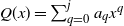 $Q(x)=\sum_{q=0}^j a_q x^q$
is any degree j polynomial.
Theorem 2. Let
 $c_n^{(\ell)}(x)$
be defined by (2); then
 $c_n^{(\ell)}(x)$
is a degree n polynomial in x. Let
 $[x^s] c_n^{(\ell)}(x)$
denote the coefficient of
 $x^s$
of the polynomial
 $c_n^{(\ell)}(x)$
; then for
 $0 \leq s \leq n$
we have
 \begin{align} \!\!\!\!\!\!\!\! [x^s] c_n^{(\ell)}(x) &= \dfrac{1}{\ell^s}\sum_{i=0}^{\min\!(s, \lfloor (n-s)/\ell \rfloor)} (\!-\!1)^i \binom{s}{i} \binom{n-i\ell}{s} \qquad \end{align}
 \begin{align} \;\;\;\;\;\;\;\;\,\quad\qquad = 1 - \dfrac{1}{\ell^s} \sum_{i=\lfloor n/\ell \rfloor +1}^s (\!-\!1)^{i+s} \binom{s}{i} \binom{s+i\ell-n-1}{s}, \end{align}
where the second expression implies that
 $[x^s] c_n^{(\ell)}(x) = 1$
for
 $s \leq \lfloor n/\ell \rfloor$
.
Proof. Expanding
 $(1+x/\ell)^{n-i(\ell+1)}$
in (2) yields
 \begin{align*}c_n^{(\ell)}(x) &= \sum_{i=0}^{\lfloor {n}/{(\ell+1)} \rfloor} (\!-\!1)^i\binom{n-i\ell}{i} \sum_{s=0}^{n-i(\ell+1)} \binom{n-i(\ell+1)}{s} \biggl(\dfrac{x}{\ell}\biggr)^{s+i}\\[5pt] &= \sum_{i=0}^{\lfloor {n}/{(\ell+1)} \rfloor} (\!-\!1)^i\binom{n-i\ell}{i} \sum_{s=i}^{n-i\ell} \binom{n-i(\ell+1)}{s-i}\dfrac{x^s}{\ell^s} \\[5pt] &= \sum_{s=0}^n \dfrac{x^s}{\ell^s} \sum_{i=0}^{\min\!(s, \lfloor (n-s)/\ell \rfloor)} (\!-\!1)^i \binom{n-i\ell}{i} \binom{n-i(\ell+1)}{s-i}.\end{align*}
The expression in (5) now follows by applying the cancellation identity, which states that
 \begin{equation*}\binom{t}{r}\binom{t-r}{a} = \binom{t}{r+a}\binom{r+a}{r},\end{equation*}
with
 $t=n-i\ell$
,
 $r=i$
, and
 $a=s-i$
.
To obtain (6) we first note that
 \begin{equation*}\dfrac{1}{\ell^s}\sum_{i=0}^s (\!-\!1)^i \binom{s}{i} \binom{n-i\ell}{s} = \dfrac{1}{\ell^s}\sum_{i=0}^s (\!-\!1)^i \binom{s}{i} \dfrac{Q(n-i\ell)}{s!} = 1,\end{equation*}
due to (4) with
 $j=s$
,
 $y=n$
,
 $\Delta=-\ell$
, and
 $Q(x)=\prod_{q=0}^{s-1} (x-q)$
. Therefore (5) implies that
 \begin{equation*}[x^s] c_n^{(\ell)}(x) =1 - \dfrac{1}{\ell^s}\sum_{i=\lfloor (n-s)/\ell \rfloor +1}^{s} (\!-\!1)^i \binom{s}{i} \binom{n-i\ell}{s}.\end{equation*}
Note that s exceeds
 $n-i\ell$
when
 $i \geq \lfloor (n-s)/\ell \rfloor +1$
. Hence
 $\binom{n-i\ell}{s}$
is zero when
 $n-i\ell \geq 0$
, that is, for
 $i \leq \lfloor n/\ell \rfloor$
, and it suffices to sum i from
 $\lfloor n/\ell \rfloor+1$
to s.
Theorem 3. The values
 $c_n^{(\ell)}(x)$
obey the following simple recursion:
 \begin{align}c_n^{(\ell)}(x) = 1 + \dfrac{x}{\ell} \sum_{j=1}^{\min\!(n,\ell)} c^{(\ell)}_{n-j}(x)\end{align}
for
 $n \geq 1$
. Further,
 \begin{align}1 = [x^0] c_n^{(\ell)}(x) \geq [x^1] c_n^{(\ell)}(x) \geq \ldots \geq [x^n] c_n^{(\ell)}(x)= \ell^{-n} \geq 0,\end{align}
 $c_n^{(\ell)}(x)$
is convex and increasing in x on
 $[0,\infty)$
and
 $c_{j\ell}^{(\ell)}(x) \geq \sum_{i=0}^{j} x^i$
.
Proof. For
 $n \leq \ell$
we have
 $c_n^{(\ell)}(x)=(1+x/\ell)^n$
, which implies that the recursion holds for
 $n \leq \ell$
. For
 $n>\ell$
, we have by (3) that
 \begin{equation*}c_n^{(\ell)}(x) - c_{n-1}^{(\ell)}(x) = \dfrac{x}{\ell} \bigl(c_{n-1}^{(\ell)}(x) - c_{n-(\ell+1)}^{(\ell)}(x) \bigr).\end{equation*}
Plugging this into
 \begin{equation*}c_n^{(\ell)}(x) - c_\ell^{(\ell)}(x) = \sum_{i=\ell+1}^n \bigl(c_i^{(\ell)}(x)-c_{i-1}^{(\ell)}(x)\bigr)\end{equation*}
yields
 \begin{align*}c_n^{(\ell)}(x) - c_\ell^{(\ell)}(x) &= \dfrac{x}{\ell} \sum_{j=1}^\ell c_{n-j}^{(\ell)}(x)- \dfrac{x}{\ell}\sum_{i=0}^{\ell-1} c_i^{(\ell)}(x)=\dfrac{x}{\ell} \sum_{j=1}^\ell c_{n-j}^{(\ell)}(x)- \bigl(c_\ell^{(\ell)}(x) - 1\bigr),\end{align*}
which proves the recursion.
Using induction on n, this recurrence together with (5) implies (8). Hence
 $c_n^{(\ell)}(x)$
is a degree n polynomial in x with non-negative coefficients and therefore all its derivatives with respect to x are non-negative on
 $[0,\infty)$
. The lower bound on
 $c_{j\ell}^{(\ell)}(x)$
follows by noting that
 $[x^s] c_{j\ell}^{(\ell)}(x) = 1$
for
 $s=0,\ldots,j$
due to Theorem 2, while
 $[x^s] c_{j\ell}^{(\ell)}(x) \geq 0$
for
 $s > j$
.
4. The M b /E k /1/m queue
We now derive results for the M
 $^b$
/E
 $_k$
/1/m queue with batch arrival rate
 $\lambda$
by relying on the following theorem by Miyazawa. We assume without loss of generality that the mean (Erlang distributed) service time of a job equals
 $1/b$
, such that the load equals
 $\lambda$
(which may exceed 1).
Theorem 4. ([Reference Miyazawa10, Theorem 2.1].) Let
 $(\psi_0,\psi_1,\ldots)$
, with
 $\psi_0 = 1$
, be the unique stationary measure of the Markov chain
 $(Y_t)_{t \geq 0}$
that keeps track of the number of jobs in an
 $\mathrm{M}^{X}/\mathrm{G}/1$
queue immediately after a service completion. The queue length distribution in an
 $\mathrm{M}^{X}/\mathrm{G}/1/m$
queue immediately after a service completion can be written as
 \begin{align*} \mathbb{P}\bigl[Q^{{M^X/G/1/ {m}}}({service}) = j\bigr] = \dfrac{\psi_j}{\sum_{i=0}^{m-1} \psi_i}\end{align*}
for
 $j=0,\ldots,m-1$
.
Miyazawa also derived a formula for the loss probability in an M
 $^X$
/G/1/m queue using the above result. This formula is, however, incorrect in the case of batch arrivals (as the probability that the server is busy should be
 $1-p^a_0 m_H$
instead of
 $1-p_0^a$
). It is easy to see that the correct formula for the loss probability in the case of batch arrivals is given by
 \begin{align*} \mathbb{P}_{\mathrm{loss}}^{{M^X/G/1/ {m}}} = 1 - \dfrac{\sum_{i=0}^{m-1} \psi_i}{m_H + \lambda\!\sum_{i=0}^{m-1} \psi_i}= 1 - \dfrac{1}{\rho} \biggl(1-\dfrac{m_H}{m_H + \lambda\!\sum_{i=0}^{m-1} \psi_i}\biggr), \end{align*}
where
 $m_H$
is the mean batch size (see also [Reference Miyazawa and Shanthikumar11, equation (3.7)]). Note that the same argument to prove Theorem 4.1 in [Reference Miyazawa10] remains valid with this corrected loss probability formula.
We are now in a position to express the queue length distribution and loss probability of the M
 $^b$
/E
 $_k$
/1/m queue in terms of the polynomials
 $c^{(kb)}_n(\lambda)$
.
Theorem 5. The loss probability
 $\mathbb{P}^\lambda_{\mathrm{loss}}(k,b,m)$
in the
 $\mathrm{M}^{b}/\mathrm{E}_{k}/1/m$
queue is given by
 \begin{align*} \mathbb{P}^\lambda_{\mathrm{loss}}(k,b,m) = 1 - \dfrac{1}{\lambda} \biggl(1-\dfrac{b}{b + \lambda \sum_{i=0}^{m-1} \psi_i^{(k,b)}(\lambda)}\biggr),\end{align*}
with
 \begin{align}\psi_i^{(k,b)}(\lambda) &= \dfrac{kb}{\lambda}\bigl(c_{ik+1}^{(kb)}(\lambda)-c_{ik}^{(kb)}(\lambda)\bigr) = c_{ik}^{(kb)}(\lambda)-c_{(i-b)k}^{(kb)}(\lambda)\end{align}
and
 \begin{align*} \sum_{i=0}^j \psi_i^{(k,b)}(\lambda) = \sum_{i=0}^{\min\!(j,b-1)} c^{(kb)}_{(j-i)k}(\lambda)\end{align*}
for
 $j \geq 0$
, where
 $c^{(\ell)}_{n}(x)$
is given by (2). The queue length distribution
 $Q_\lambda^{(k,b,m)}$
can be expressed as
 \begin{equation*} \mathbb{P}\bigl[Q_\lambda^{(k,b,m)} \leq j\bigr] = \dfrac{b c_{jk}^{(kb)}(\lambda)}{b+\lambda \sum_{i=0}^{m-1} \psi_i^{(k,b)}(\lambda)}\end{equation*}
for
 $j=0,\ldots,m-1$
.
Proof. If we keep track of the number of phases present in the M
 $^b$
/E
 $_k$
/1 queue, we obtain the Markov chain
 $\bigl(X^{(\ell,x)}_t\bigr)_{t \geq 0}$
with
 $x=\lambda$
,
 $\ell=kb$
and
 $q=1$
. Theorem 1 therefore implies that
 \begin{equation*}p_n^{(kb)}(\lambda) = c_n^{(kb)}(\lambda) - c_{n-1}^{(kb)}(\lambda)\end{equation*}
is a stationary measure for this chain.
The queue length becomes i after a service completion from state
 $ik+1$
. Therefore the measure
 $\psi_i^{(k,b)}(\lambda)$
used in Theorem 4 is proportional to
 $p_{ik+1}^{(kb)}(\lambda)$
and is given by
 \begin{align}\psi_i^{(k,b)}(\lambda) = \dfrac{kb}{\lambda} \bigl(c^{(kb)}_{ik+1}(\lambda)-c^{(kb)}_{ik}(\lambda)\bigr),\end{align}
where the factor
 $kb/\lambda$
is such that
 $\psi_0^{(k,b)}(\lambda) = 1$
. From (7) we note that
 \begin{align*}c^{(kb)}_{ik+1}(\lambda)-c^{(kb)}_{ik}(\lambda) =\dfrac{\lambda}{kb} \bigl(c^{(kb)}_{ik}(\lambda)-c^{(kb)}_{(i-b)k}(\lambda)\bigr)\end{align*}
for
 $i \geq b$
, and
 \begin{align*}c^{(kb)}_{ik+1}(\lambda)-c^{(kb)}_{ik}(\lambda) =\dfrac{\lambda}{kb} c^{(kb)}_{ik}(\lambda)\end{align*}
for
 $i < b$
. These equalities can be combined with (10) to yield (9). It is now easy to verify that
 \begin{align*}\sum_{i=0}^j \psi_i^{(k,b)}(\lambda) = \sum_{i=0}^{\min\!(j,b-1)} c^{(kb)}_{(j-i)k}(\lambda).\end{align*}
Further, by Theorem 4 and (2.9) in [Reference Miyazawa10] we have
 \begin{equation*} \mathbb{P}\bigl[Q_\lambda^{(k,b,m)}({arrival}) = j\bigr] = \dfrac{ \psi_j^{(k,b)}(\lambda)}{b+\lambda \sum_{i=0}^{m-1} \psi_i^{(k,b)}(\lambda)}\end{equation*}
for
 $j=0,\ldots,m-1$
. Note that this is the queue length distribution just prior to a job arrival. In the case of batch arrivals, the
 $i-1$
jobs preceding the ith job of a batch are also considered as being part of the queue just before the arrival of the ith job.
As the arrivals occur in batches of size b, we have
 \begin{equation*}\mathbb{P}\bigl[Q_\lambda^{(k,b,m)}({arrival}) = j\bigr] = \sum_{i=0}^{\min\!(j,b-1)} \dfrac{1}{b} \mathbb{P}\bigl[Q_\lambda^{(k,b,m)} = j-i\bigr]. \end{equation*}
This implies that
 \begin{align*}&\mathbb{P}\bigl[Q_\lambda^{(k,b,m)}({arrival}) = j\bigr] - \mathbb{P}\bigl[Q_\lambda^{(k,b,m)}({arrival}) = j-1\bigr]\\[5pt] &\quad = \dfrac{1}{b} \bigl(\mathbb{P}\bigl[Q_\lambda^{(k,b,m)} = j\bigr] - \mathbb{P}\bigl[Q_\lambda^{(k,b,m)} = j-b\bigr] 1[j \geq b]\bigr).\end{align*}
Reordering yields the recursion
 \begin{align*} \mathbb{P}\bigl[Q_\lambda^{(k,b,m)} = j\bigr] & = b \mathbb{P}\bigl[Q_\lambda^{(k,b,m)}({arrival}) = j\bigr] - b \mathbb{P}\bigl[Q_\lambda^{(k,b,m)}({arrival}) = j-1\bigr] \\[5pt] &\quad + \mathbb{P}\bigl[Q_\lambda^{(k,b,m)} = j-b\bigr]1[j \geq b]. \end{align*}
Hence
 \begin{align*} \mathbb{P}\bigl[Q_\lambda^{(k,b,m)} = j\bigr] &= b \sum_{i=0}^{\lfloor j/b \rfloor} \bigl(\mathbb{P}\bigl[Q_\lambda^{(k,b,m)}({arrival}) = j-ib\bigr] - \mathbb{P}\bigl[Q_\lambda^{(k,b,m)}({arrival}) = j-ib-1\bigr]\bigr) \\[5pt] &= \dfrac{b \sum_{i=0}^{\lfloor j/b \rfloor} \bigl(\psi_{j-ib}^{(k,b)}(\lambda)-\psi_{j-ib-1}^{(k,b)}(\lambda)\bigr)}{b+\lambda \sum_{i=0}^{m-1} \psi_i^{(k,b)}(\lambda)}, \end{align*}
with
 $\psi_{-1}^{(k,b)}(\lambda)=0$
. Finally, (9) implies that
 \begin{equation*} c_{jk}^{(kb)}(\lambda) = \psi_{j}^{(k,b)}(\lambda) + c_{jk-bk}^{(kb)}(\lambda),\end{equation*}
which can be used to show that
 \begin{equation*} c_{jk}^{(kb)}(\lambda) = \sum_{i=0}^{\lfloor j/b \rfloor} \psi_{j-ib}^{(k,b)}(\lambda),\end{equation*}
and similarly as
 $ \psi_{-1}^{(k,b)}(\lambda)=0$
 \begin{equation*} c_{(j-1)k}^{(kb)}(\lambda) = \sum_{i=0}^{\lfloor j/b \rfloor} \psi_{j-ib-1}^{(k,b)}(\lambda).\end{equation*}
Therefore
 \begin{align*} \mathbb{P}\bigl[Q_\lambda^{(k,b,m)} = j\bigr] &= \dfrac{b \bigl( c_{jk}^{(kb)}(\lambda)-c_{(j-1)k}^{(kb)}(\lambda)\bigr)}{b+\lambda \sum_{i=0}^{m-1} \psi_i^{(k,b)}(\lambda)}, \end{align*}
We now focus on two special cases: the M/E
 $_k$
/1/m queue and the M
 $^b$
/M/1/m queue.
Corollary 2. The loss probability
 $\mathbb{P}^\lambda_{\mathrm{loss}}(k,1,m)$
in an
 $\mathrm{M}/\mathrm{E}_{k}/1/m$
queue is given by
 \begin{align*} \mathbb{P}^\lambda_{\mathrm{loss}}(k,m) = 1 - \dfrac{1}{\lambda}\biggl( 1 - \dfrac{1}{1+\lambda c_{(m-1)k}^{(k)}(\lambda)}\biggr),\end{align*}
where
 $c^{(k)}_{(m-1)k}(\lambda)$
is given by (2). The queue length distribution can be expressed as
 \begin{equation*} \mathbb{P}\bigl[Q_\lambda^{(k,1,m)} \leq j\bigr] = \dfrac{c_{jk}^{(k)}(\lambda)}{1+\lambda c_{(m-1)k}^{(k)}(\lambda)}\end{equation*}
for
 $j=0,\ldots,m-1$
.
Proof. Setting
 $b=1$
implies that
 \begin{equation*} \sum_{i=0}^j \psi_i^{(k,1)}(\lambda) = c_{jk}^{(k)}(\lambda). \end{equation*}
Corollary 3. The loss probability
 $\mathbb{P}_{\mathrm{loss}}(1,b,m)$
in an
 $\mathrm{M}^{b}/\mathrm{M}/1/m$
queue is given by
 \begin{align*} \mathbb{P}^\lambda_{\mathrm{loss}}(1,b,m) = 1 - \dfrac{1}{\lambda}\biggl( 1 - \dfrac{1}{c_{m}^{(b)}(\lambda)}\biggr),\end{align*}
where
 $c^{(b)}_{m}(\lambda)$
is given by (2). The queue length distribution can be expressed as
 \begin{equation*} \mathbb{P}\bigl[Q_\lambda^{(1,b,m)} \leq j\bigr] = \dfrac{c_{j}^{(b)}(\lambda)}{c_{m}^{(b)}(\lambda)}\end{equation*}
for
 $j=0,\ldots,m$
.
Proof. Setting
 $k=1$
immediately implies that
 \begin{equation*}\psi_i^{(1,b)}(\lambda) = b \bigl(c^{(b)}_{i+1}(\lambda)-c^{(b)}_{i}(\lambda)\bigr)/\lambda\end{equation*}
and therefore
 \begin{equation*} \sum_{i=0}^j \psi_i^{(1,b)}(\lambda) = b \bigl(c^{(b)}_{j+1}(\lambda)-1\bigr)/\lambda. \end{equation*}
5. The E k /M b /1/m queue
Consider the E
 $_k$
/M
 $^b$
/1/m queue with arrival rate
 $\lambda$
and a mean batch service rate
 $1/b$
, such that the load equals
 $\lambda$
. To express the queue length distribution and loss probability we rely on the following duality result by Miyazawa.
Theorem 6. ([Reference Miyazawa10, Theorem 3.1].) Let
 $(\phi_0,\phi_1,\ldots)$
, with
 $\phi_0 = 1$
, be the unique stationary measure of the Markov chain
 $(Z_t)_{t \geq 0}$
that keeps track of the number of jobs in a modified
 $\mathrm{M}^{X}/\mathrm{G}/1$
queue immediately after a service completion where the modification is such that the batch size equals one when the queue is empty. Let
 $\lambda$
be the batch arrival rate and G the service time distribution.
The queue length distribution in a GI/M
 $^X$
/1/m queue with inter-arrival time distribution G and batch service rate
 $\lambda$
just prior to an arrival can be written as
 \begin{align*} \mathbb{P}\bigl[Q^{{GI/M^X/1/ {m}}}({arrival}) = j\bigr] = \dfrac{\phi_{m-j}}{\sum_{i=0}^{m} \phi_i}\end{align*}
for
 $j=0,\ldots,m$
.
Lemma 1. Let
 \begin{equation*} \bigl(\phi_0^{(k,b)}(x),\phi_1^{(k,b)}(x),\ldots\bigr), \end{equation*}
with
 $\phi_0^{(k,b)}(x) = 1$
, be the unique stationary measure of the Markov chain
 $\bigl(Z^{(k,b,x)}_t\bigr)_{t \geq 0}$
that keeps track of the number of jobs in a modified
 $\mathrm{M}^{b}/\mathrm{E}_{k}/1$
queue with load x immediately after a service completion where the modification is such that the batch size equals one when the queue is empty. Then
 \begin{align*} \phi_i^{(k,b)}(x) = c_{ik}^{(kb)}(x)-c_{(i-1)k}^{(kb)}(x) \end{align*}
for
 $i\geq 0$
.
Proof. The stationary measure of the M
 $^X$
/G/1 queue without the modification is given by (9). The expression for the complementary generating functions in (2.7) in [Reference Miyazawa10] implies that for
 $0 < z < z_0$
, for some
 $z_0$
sufficiently small,
 \begin{align*}\sum_{i=0}^\infty \phi_i^{(k,b)}(x) z^i &=\dfrac{1-z}{1-z^b}\sum_{i=0}^\infty \psi_i^{(k,b)}(x) z^i= \sum_{i=0}^\infty \psi_i^{(k,b)}(x) z^i (1-z)\sum_{j=0}^\infty z^{bi},\end{align*}
which yields
 \begin{equation*} \phi_i^{(k,b)}(x) = \sum_{j=0}^{\lfloor i/b \rfloor}\psi_{i-jb}^{(k,b)}(x) - \sum_{j=0}^{\lfloor (i-1)/b \rfloor}\psi_{i-jb-1}^{(k,b)}(x). \end{equation*}
Combined with (9) this proves the statement.
Lemma 2. The polynomials defined by (2) obey the following equality:
 \begin{align*} \sum_{i=0}^{k-1}c_{jk+i}^{(kb)}(x) = \dfrac{kb}{x}\sum_{i=0}^{\lfloor j/b \rfloor} \bigl(c_{(j+1)k-ibk}^{(kb)}(x)-c_{jk-ibk}^{(kb)}(x)\bigr)\end{align*}
for
 $k,b > 0$
and
 $j \geq 0$
.
Proof. By (3) we have
 \begin{equation*}c_{n-i\ell+1}^{(\ell)}(x)-c_{n-i\ell}^{(\ell)}(x) =\dfrac{x}{\ell} \bigl(c_{n-i\ell}^{(\ell)}(x)-c_{n-(i+1)\ell}^{(\ell)}(x)\bigr) \end{equation*}
for
 $n-i\ell+1 > 0$
. Summing over i then yields
 \begin{equation*}c_n^{(\ell)}(x) = \dfrac{\ell}{x} \sum_{i=0}^{\lfloor n/\ell \rfloor}\bigl(c_{n-i\ell+1}^{(\ell)}(x)-c_{n-i\ell}^{(\ell)}(x)\bigr)\end{equation*}
as
 $c_{n-\ell-\lfloor n/\ell \rfloor\ell}^{(\ell)}(x)=0$
. Setting
 $\ell = kb$
and
 $n=jk$
, we therefore have
 \begin{align*}\sum_{s=0}^{k-1}c_{jk+s}^{(kb)}(x) &= \dfrac{kb}{x} \sum_{s=0}^{k-1}\sum_{i=0}^{\lfloor (jk+s)/kb \rfloor}\bigl(c_{jk+s-ikb+1}^{(kb)}(x)-c_{jk+s-ikb}^{(kb)}(x)\bigr) \\[5pt]&= \dfrac{kb}{x}\sum_{i=0}^{\lfloor j/b \rfloor}\sum_{s=0}^{k-1}\bigl(c_{jk+s-ikb+1}^{(kb)}(x)-c_{jk+s-ikb}^{(kb)}(x)\bigr) \\[5pt]&= \dfrac{kb}{x}\sum_{i=0}^{\lfloor j/b \rfloor}\bigl(c_{jk-ikb+k}^{(kb)}(x)-c_{jk-ikb}^{(kb)}(x)\bigr),\end{align*}
where the second equality holds as
 $\lfloor (jk+s)/kb \rfloor = \lfloor \,j/b \rfloor$
for
 $s \in \{0,\ldots,k-1\}$
.
Theorem 7. The loss probability
 $\tilde{\mathbb{P}}^\lambda_{\mathrm{loss}}(k,b,m)$
in the
 $\mathrm{E}_k/\mathrm{M}^b/1/m$
queue with load
 $\lambda$
is given by
 \begin{align*} \tilde{\mathbb{P}}^\lambda_{\mathrm{loss}}(k,b,m) = \dfrac{1}{c_{mk}^{(kb)}(1/\lambda)}.\end{align*}
The queue length distribution is given by
 \begin{equation*}\mathbb{P}\bigl[\tilde Q_\lambda^{(k,b,m)} \geq m-j\bigr] = \dfrac{\sum_{i=0}^{k-1}c_{jk+i}^{(kb)}(1/\lambda)}{k c_{mk}^{(kb)}(1/\lambda)}\end{equation*}
for
 $j=0,\ldots,m-1$
.
Proof. The loss formula follows by combining Theorem 6 with Lemma 1, where we note that the M
 $^b$
/E
 $_k$
/1 queue has load
 $1/\lambda$
if the dual E
 $_k$
/M
 $^b$
/1/m queue has load
 $\lambda$
.
By Theorem 6, (2.9) in [Reference Miyazawa10] and Lemma 1, we have for
 $j=0,\ldots,m-1$
 \begin{equation*} \mathbb{P}\bigl[\tilde Q_\lambda^{(k,b,m)}({service}) = j\bigr] = \dfrac{c_{(m-j)k}^{(kb)}(1/\lambda)-c_{(m-j-1)k}^{(kb)}(1/\lambda)}{c_{mk}^{(kb)}(1/\lambda)-1},\end{equation*}
where
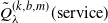 $\tilde Q_\lambda^{(k,b,m)}({service})$
represents the queue length immediately after a job completion in an E
 $_k$
/M
 $^b$
/1/m queue, where the
 $b-i$
jobs after the ith job of a batch are still counted as present in the queue when the ith job completes service.
As the batch service completions occur at rate
 $1/b$
, we have
 \begin{align*}&\mathbb{P}\bigl[\tilde Q_\lambda^{(k,b,m)}({service}) = m-j\bigr] = \dfrac{\mathbb{P}\bigl[m-j+1 \leq \tilde Q_\lambda^{(k,b,m)} \leq \min\!(m-j+b,m)\bigr]}{b\lambda\bigl(1-\tilde P^\lambda_{\mathrm{loss}}(k,b,m)\bigr)}\end{align*}
for
 $j=1,\ldots,m$
. Combining the previous two equations with the expression for
 $\tilde P^\lambda_{\mathrm{loss}}(k,b,m)$
shows that
 \begin{equation*} \mathbb{P}\bigl[m-j+1 \leq \tilde Q_\lambda^{(k,b,m)} \leq \min\!(m-j+b,m)\bigr] =\dfrac{\lambda b \bigl(c_{jk}^{(kb)}(1/\lambda)-c_{(j-1)k}^{(kb)}(1/\lambda)\bigr)}{c_{mk}^{(kb)}(1/\lambda)} \end{equation*}
for
 $j=0,\ldots,m-1$
. The probability
 $\mathbb{P}\bigl[\tilde Q_\lambda^{(k,b,m)} \geq m-j\bigr]$
can therefore be expressed as
 \begin{align*}\mathbb{P}\bigl[\tilde Q_\lambda^{(k,b,m)} \geq m-j\bigr] & = \sum_{i=0}^{\lfloor j/b \rfloor} \mathbb{P}\bigl[m-j-ib \leq \tilde Q_\lambda^{(k,b,m)} \leq \min\!(m-j-ib+b-1,m)\bigr] \\[5pt] & = \dfrac{\lambda b}{c_{mk}^{(kb)}(1/\lambda)} \sum_{i=0}^{\lfloor j/b \rfloor} \bigl(c_{((j+1)-ib)k}^{(kb)}(1/\lambda)-c_{(j-ib)k}^{(kb)}(1/\lambda)\bigr)\end{align*}
for
 $j=0,\ldots,m-1$
. The proof is now completed by applying Lemma 2 with
 $x=1/\lambda$
.
We now focus on two special cases: the E
 $_k$
/M/1/m queue and the M/M
 $^b$
/1/m queue.
Corollary 4. The loss probability
 $\tilde{\mathbb{P}}^\lambda_{\mathrm{loss}}(k,1,m)$
in an E
 $_k$
/M/1/m queue is given by
 $1/c_{mk}^{(k)}(1/\lambda)$
, where
 $c^{(\ell)}_{n}(x)$
is given by (2). The queue length distribution can be expressed as
 \begin{equation*} \mathbb{P}\bigl[\tilde Q_\lambda^{(k,1,m)} \geq m-j\bigr] =\dfrac{\lambda \bigl(c_{(j+1)k}^{(k)}(1/\lambda)-1\bigr)}{c_{mk}^{(k)}(1/\lambda)}\end{equation*}
for
 $j=0,\ldots,m-1$
.
Proof. Setting
 $b=1$
implies that
 \begin{align*}\mathbb{P}\bigl[\tilde Q_\lambda^{(k,1,m)} \geq m-j\bigr] &= \dfrac{\sum_{i=0}^{k-1}c_{jk+i}^{(k)}(1/\lambda)}{k c_{mk}^{(k)}(1/\lambda)}=\dfrac{\lambda \bigl(c_{(j+1)k}^{(k)}(1/\lambda)-1\bigr)}{c_{mk}^{(k)}(1/\lambda)},\end{align*}
due to (3) with
 $\ell = k$
and
 $x=1/\lambda$
.
Corollary 5. The loss probability
 $\tilde{\mathbb{P}}_{\mathrm{loss}}(1,b,m)$
in an
 $\mathrm{M}/\mathrm{M}^{b}/1/m$
queue is given by
 $1/c_{m}^{(b)}(1/\lambda)$
, where
 $c^{(\ell)}_{n}(x)$
is given by (2). The queue length distribution can be expressed as
 \begin{equation*} \mathbb{P}\bigl[\tilde Q_\lambda^{(1,b,m)} \geq m-j\bigr] = \dfrac{c_{j}^{(b)}(1/\lambda)}{c_{m}^{(b)}(1/\lambda)}\end{equation*}
for
 $j=0,\ldots,m$
.
Proof. Setting
 $k=1$
in Theorem 7 yields the result.
It is worth noting that the loss probabilities of the E
 $_k$
/M/1/m queue and the M/M
 $^k$
/1/mk queue are identical, even though their associated finite-state Markov chains are not.
6. The M b /D/1/m and D/M b /1/m queues
We now present closed-form results for the M
 $^b$
/D/1/m and D/M
 $^b$
/1/m queues. Setting
 $b=1$
in the M
 $^b$
/D/1/m queue yields the results in [Reference Brun and Garcia3] (as
 $\xi_j(\lambda)$
corresponds to
 $b_j$
in [Reference Brun and Garcia3]).
Theorem 8. The loss probability
 $\mathbb{P}^\lambda_{\mathrm{loss}}(\infty,b,m)$
in the
 $\mathrm{M}^{b}/\mathrm{D}/1/m$
queue is given by
 \begin{align*} \mathbb{P}^\lambda_{\mathrm{loss}}(\infty,b,m) = 1 - \dfrac{1}{\lambda} \biggl(1-\dfrac{b}{b + \lambda \sum_{i=0}^{\min\!(b-1,m-1)} \xi_{(m-1-i)/b}(\lambda)}\biggr),\end{align*}
with
 \begin{align}\xi_y(x) =\sum_{i=0}^{\lfloor y \rfloor} \dfrac{(\!-\!1)^i x^i}{i!}(y-i)^i \,{\mathrm{e}}^{x(y-i)}\end{align}
for
 $y \geq 0$
real. The queue length distribution
 $Q_\lambda^{(\infty,b,m)}$
can be expressed as
 \begin{equation*} \mathbb{P}\bigl[Q_\lambda^{(\infty,b,m)} \leq j\bigr] = \dfrac{b \xi_{j/b}(\lambda)}{b+\lambda \sum_{i=0}^{\min\!(m-1,b-1)} \xi_{(m-1-i)/b}(\lambda)}\end{equation*}
for
 $j=0,\ldots,m-1$
.
Proof. The result follows from Theorem 5 by letting k tend to infinity and noting that
 $\xi_{j/b}(\lambda) = \lim_{k \rightarrow \infty} c^{(kb)}_{jk}(\lambda) $
.
Theorem 9. The loss probability
 $\tilde{\mathbb{P}}^\lambda_{\mathrm{loss}}(\infty,b,m)$
in the
 $\mathrm{D}/\mathrm{M}^{b}/1/m$
queue is given by
 \begin{align*} \tilde{\mathbb{P}}^\lambda_{\mathrm{loss}}(\infty,b,m) = \dfrac{1}{\xi_{m/b}(1/\lambda)},\end{align*}
where
 $\xi_y(x)$
is given by (11). The queue length distribution
 $\tilde Q_\lambda^{(\infty,b,m)}$
can be expressed as
 \begin{equation*} \mathbb{P}\bigl[\tilde Q_\lambda^{(\infty,b,m)} \geq m-j\bigr] = \dfrac{\lambda b \!\sum_{i=0}^{\lfloor j/b \rfloor}(\xi_{(j+1)/b-i}(1/\lambda)-\xi_{j/b-i}(1/\lambda))}{\xi_{m}^{(b)}(1/\lambda)}\end{equation*}
for
 $j=0,\ldots,m-1$
.
7. Some finite capacity fluid queues
In this section we present results for the following two fluid queues. In both queues we have a buffer with capacity m. In the first queueing system fluid drains from the queue at rate 1 and arrivals occur at rate
 $\lambda$
that instantaneously add one unit of fluid to the buffer unless the fluid in the buffer exceeds
 $m-1$
, in which case the fluid level becomes m. Note that this fluid queue corresponds to the work present in an M/D/1 queue with bounded workload and partial acceptance.
The second queueing system is the dual of the first, where the fluid level increases at rate
 $\lambda$
and Poisson arrivals at rate 1 instantaneously remove one unit of fluid from the buffer or empty the buffer if the fluid is below 1. We denote these queueing systems as the fluid M/D/1 and fluid D/M/1 queues, respectively.
Corollary 6. The fraction of lost work in the fluid M/D/1 queue is given by
 \begin{equation*} \lim_{b \rightarrow \infty} \mathbb{P}^\lambda_{\mathrm{loss}}(1,b,bm) = 1 - \dfrac{1}{\lambda} \biggl( 1 - \dfrac{1}{\xi_m(\lambda)} \biggr),\end{equation*}
where
 $\xi_y(x)$
is defined in (11). The probability that the fluid level is at most
 $y \in [0,m]$
is given by
 $\xi_y(\lambda)/\xi_m(\lambda)$
.
Proof. The fluid M/D/1 queue is equivalent to the M
 $^b$
/M/1/bm queue if we let b tend to infinity and renormalize the buffer size by b; then the result follows from Corollary 3 and the fact that
 $\xi_y(x) = \lim_{b \rightarrow \infty} c^{(b)}_{by}(x)$
.
Corollary 7. The fraction of lost fluid in the fluid D/M/1 queue is given by
 \begin{equation*} \lim_{b \rightarrow \infty} \tilde{\mathbb{P}}^\lambda_{\mathrm{loss}}(1,b,bm) = \dfrac{1}{\xi_m(1/\lambda)},\end{equation*}
where
 $\xi_y(x)$
is defined in (11). The probability that the fluid level exceeds
 $m-y$
with
 $y \in [0,m]$
is given by
 $\xi_y(1/\lambda)/\xi_m(1/\lambda)$
.
Proof. The fluid D/M/1 queue is equivalent to the M/M
 $^b$
/1/bm queue if we let b tend to infinity and renormalize the buffer size by b; then the result follows from Corollary 5 and the fact that
 $\xi_y(x) = \lim_{b \rightarrow \infty} c^{(b)}_{by}(x)$
.
Note that the above results are also valid if m is not an integer.
8. Conclusions
In this paper we have presented simple analytical expressions for the M
 $^b$
/E
 $_k$
/1/m and E
 $_k$
/M
 $^b$
/1/m queues as well as for some closely related queueing systems. We demonstrated that both the loss probability and queue length distribution can be expressed in terms of the polynomials
 $c_n^{\ell}(x)$
given by (2).
We further note that these polynomials can also be used to obtain analytical expressions for other queueing systems not considered in this paper, such as the M/M
 $^b$
/1/m queue where the server is interrupted if the number of jobs in the system is below b. It may also be possible to extend some of the results in this paper to multi-server systems.
Funding information
This work was supported by the FWO-Flanders project G033119N.
Competing interests
There were no competing interests to declare which arose during the preparation or publication process of this article.



