1 Introduction
In the early years of the development of shear flow stability theory, asymptotic analysis was the only tool available to researchers that proved able to produce quantitative theoretical results. Plane Poiseuille flow (PPF), the flow through a two-dimensional channel subject to a fixed pressure gradient, was chosen in many mathematical analyses because of its simplicity. A theoretical attempt to find the critical Reynolds number for this flow can be found as early as Heisenberg (Reference Heisenberg1924). His analysis was extended by Lin (Reference Lin1945, Reference Lin1955), who completed the description of the linear neutral curve by the method of matched asymptotic expansions, addressing the large-Reynolds-number limit in order to derive a reduced form of governing equations. At first glance this limiting process appears simple as it corresponds to the vanishing of viscosity. However, the singular behaviour of the inviscid dynamics requires the analysis of small-scale structures in the critical layer (where the phase speed of the instability wave and basic velocity coincide) and in near-wall boundary layers. Mutual interaction of the small- and large-scale structures occurs through the ‘matching’, which plays a crucial role in deriving a closed reduced system in the large-Reynolds-number asymptotic limit.
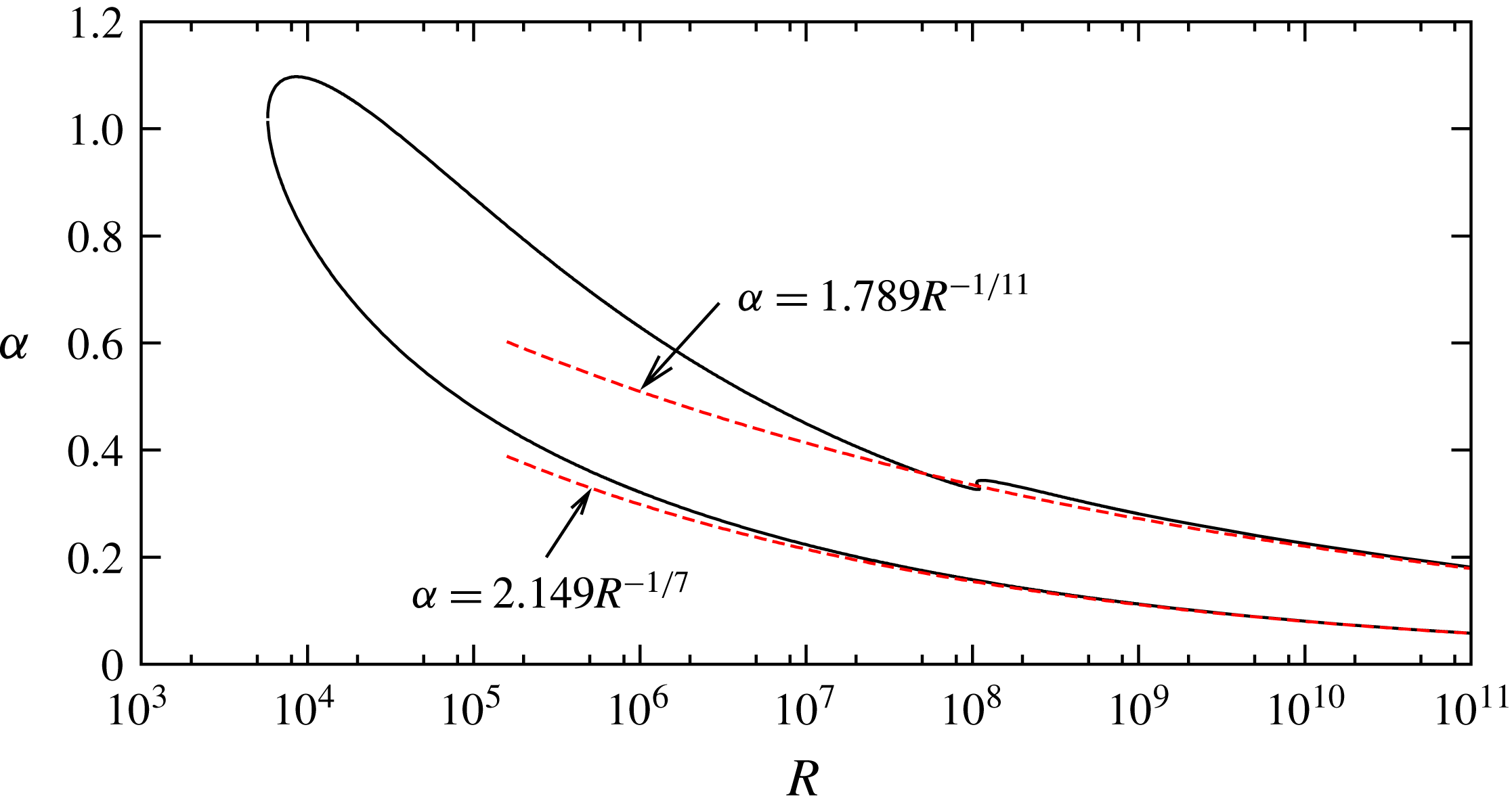
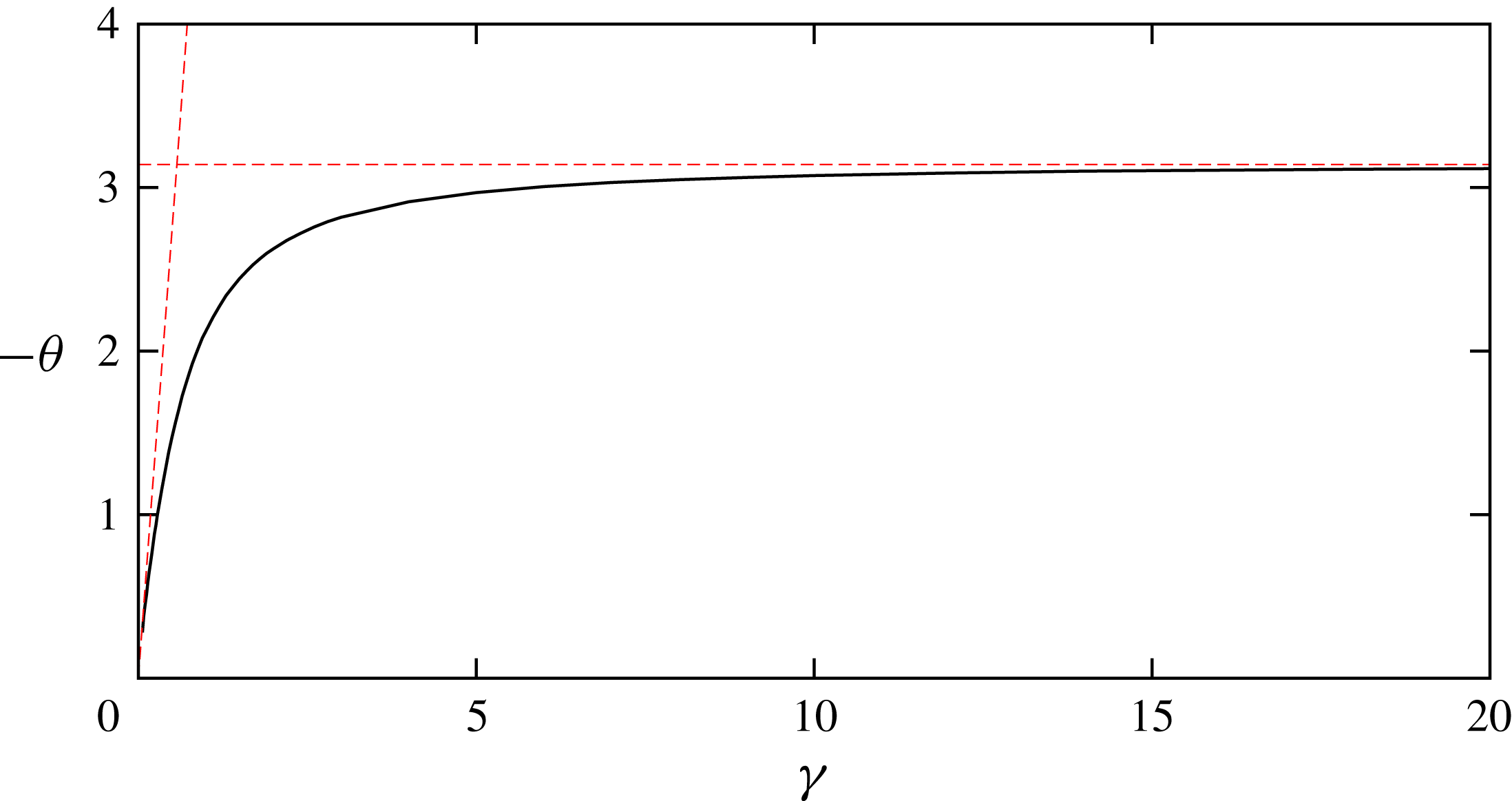
The linear neutral curve for plane Poiseuille flow. The two red dashed curves are the asymptotic results (Lin Reference Lin1945, Reference Lin1955). Those lower and upper asymptotic curves are re-derived in this paper, as given in (4.23) and (5.21), respectively.

Advances in computing technology eventually led to the development of sophisticated numerical techniques as an alternative tool to the asymptotic approach, as exemplified by Orszag’s (Reference Orszag1971) solution of the linearised Navier–Stokes equations for channel flow using a spectral method. Nowadays the neutral curve of PPF can easily be found, as shown in figure 1. In the figure
 $R$
is the Reynolds number (based on half-channel width and centreline velocity), while
 $\unicode[STIX]{x1D6FC}$
is the non-dimensional streamwise wavenumber, also scaled on the half-channel width. The neutral curve, shown by the black solid curve, appears at the well-known critical value
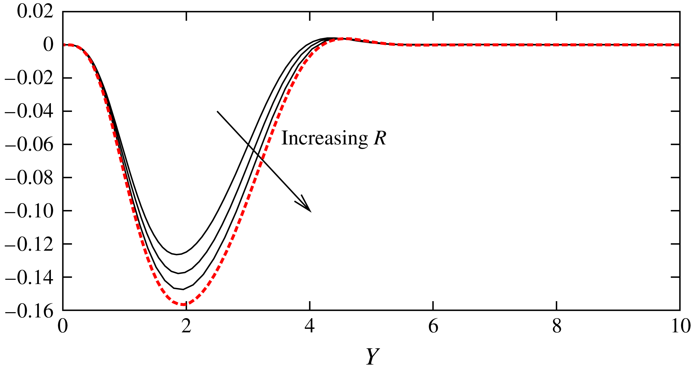
 $R\simeq 5772$
, with this critical location representing the meeting point of the upper and lower branches. It has been established (see, for example, Drazin & Reid (Reference Drazin and Reid1981)) that the asymptotic results obtained earlier by the theoreticians give excellent approximations for the large-Reynolds-number fate of the two branches of the neutral curve: see the dashed curves in the figure.
As is clear from this example, asymptotic theory is a powerful tool that can be used to produce convincing quantitative large-Reynolds-number predictions with minimal assumption. Remarkably, all coefficients in the asymptotic prediction can be found by solving reduced problems independent of Reynolds number, and in fact the method is the only known way to produce such a closure without the need for artificial assumptions and/or tuning parameters. Moreover, the physical mechanism of the instability can be elucidated in the most natural way. It became clear from Lin’s theory that the mechanism underpinning the neutral curve is the same kind of instability as the Tollmien–Schlichting (TS) wave observed in boundary layers (Tollmien Reference Tollmien1929; Schlichting Reference Schlichting1933). This type of instability is particularly important when the disturbance amplitude is small (see, for example, experimental work by Nishioka, Iida & Ichikawa (Reference Nishioka, Iida and Ichikawa1975)).
Our aim in this paper is to demonstrate how the theoretical results and their successful validation by Navier–Stokes computations seen in the linear regime can be extended to incorporate the effects of nonlinearity. Significant recent advances in computational power allow us to study the instability of shear flows even when the disturbance amplitude is relatively high. Recently, nonlinear equilibrium solutions of the Navier–Stokes equations and their large-Reynolds-number development has become an area of concentrated research. The numerical investigation of such solutions is at the forefront of this activity in view of the crucial role that they play in laminar–turbulent transition and developed turbulence (see, for example, Kawahara, Uhlmann & van Veen (Reference Kawahara, Uhlmann and van Veen2012)). In an analogous fashion to the linear case, various large-Reynolds-number asymptotic theories give a surprisingly good prediction for the Reynolds number dependence of Navier–Stokes solutions. However, most of the previous works in this direction of research are concerned with three-dimensional structures. For example, Hall & Sherwin (Reference Hall and Sherwin2010) showed that when the Reynolds number is increased, three-dimensional solutions of plane Couette flow converge to the vortex/Rayleigh wave interaction states formulated by Hall & Smith (Reference Hall and Smith1991). The nonlinear interaction of streamwise vortices and the predominantly inviscid wave within the critical layer explains rationally the emergence of a roll–streak structure frequently observed numerically and experimentally at finite Reynolds number (see, for example, Waleffe (Reference Waleffe1997)). Subsequently, Dempsey et al. (Reference Dempsey, Deguchi, Hall and Walton2016) confirmed the presence of a similar roll/streak/wave interaction in PPF, but with the wave being of three-dimensional TS wave type, with the appropriate interaction equations originally derived by Bennett, Hall & Smith (Reference Bennett, Hall and Smith1991). It has also been established that the effective Reynolds number for the wave becomes of order unity for extremely large/small wavenumbers or at the edge of boundary layer flows. In these cases a ‘regular’ class of asymptotic states occurs that does not depend on the critical layer singularity (see Deguchi, Hall & Walton (Reference Deguchi, Hall and Walton2013), Deguchi & Hall (Reference Deguchi and Hall2014a ), Deguchi (Reference Deguchi2015)).
TS waves are essentially two-dimensional and therefore the roll/streak/wave-type interaction theories are not directly applicable. However, self-consistent two-dimensional asymptotic theories for nonlinear travelling waves are well-established near both branches of the neutral curve. The fundamental previous work used in the self-consistent asymptotic theories is due to Benney & Bergeron (Reference Benney and Bergeron1969) and Davis (Reference Davis1969), who recognised that, in the critical layer, a disturbance of sufficiently large amplitude is essentially governed by inviscid dynamics. In order to determine the amplitude dependence of the neutral modes, a thorough analysis of the critical layer proves vital. Haberman (Reference Haberman1972, Reference Haberman1976) and Brown & Stewartson (Reference Brown and Stewartson1978) showed how this layer was influenced by the inclusion of weak nonlinearity and viscosity, leading to a phase shift of the wave and an enhanced velocity jump across it for a given amplitude. Viscosity remains an important effect in all these theories, with the amplitude dependence determined by the balancing of the viscous-induced mean velocity jump across the critical layer with that produced by a steady-streaming effect within the wall layer. Smith & Bodonyi (Reference Smith and Bodonyi1982a ) and Bodonyi, Smith & Gajjar (Reference Bodonyi, Smith and Gajjar1983), using as a basis the asymptotic structure governing linear disturbances near the upper neutral branch, formalised this work and extended it to the situation where the critical layer becomes strongly nonlinear and moves away from the boundary. Much of this ‘nonlinear critical layer theory’ was formulated originally in the context of boundary layer flows, but can easily be extended to parallel flows in channels (Bodonyi et al. Reference Bodonyi, Smith and Gajjar1983), pipes (Smith & Bodonyi Reference Smith and Bodonyi1982b ; Deguchi & Walton Reference Deguchi and Walton2013a ) and annular geometries (Walton Reference Walton2003; Deguchi & Walton Reference Deguchi and Walton2013b ), with the latter two Deguchi–Walton papers demonstrating the excellent agreement between the asymptotics and 2D Navier–Stokes computations, provided the Reynolds number is sufficiently large.
On the lower branch the fundamental asymptotic structure has a triple-deck form for boundary layers, as was first recognised by Smith (Reference Smith1979a ), with an analogous double-deck structure in place for channels (Smith Reference Smith1979b ). Drawing on the ideas of Stuart (Reference Stuart1960), who famously formulated weakly nonlinear stability theory for PPF at finite values of the Reynolds number, Hall & Smith (Reference Hall and Smith1982) derived the analogous Landau amplitude equation for disturbances that become nonlinear close to the lower branch at asymptotically large Reynolds number. Interestingly, this theory predicts a subcritical bifurcation so that nonlinearity is a destabilising effect: this is in contrast to large, but finite, weakly nonlinear analyses, where the bifurcation from the lower branch is found to be supercritical (Itoh Reference Itoh1974) (see also the numerical results in § 2 of this paper). In the context of the development of boundary layers, Smith & Burggraf (Reference Smith and Burggraf1985) considered theoretically the nonlinear form of the triple-deck structure and proposed a new asymptotic structure that may replace it at higher amplitude. Subsequently, Hall (Reference Hall1995) showed that this so-called ‘Euler stage’ was apparently unreachable from the computation of travelling wave states of the triple-deck equations at increasing amplitude.
Given the amount of effort expended in showing theoretically how these nonlinear structures emerge with increasing amplitude from the corresponding linear asymptotic states, there has been surprisingly little attempt to demonstrate this development by comparison with Navier–Stokes solutions. As mentioned earlier, excellent agreement of this kind was found in the strongly nonlinear critical layer regime by Deguchi & Walton (Reference Deguchi and Walton2013a ,Reference Deguchi and Walton b ) for axisymmetric sliding Couette flow and spiral waves in pipe flow. However, the agreement can only be seen along a section of the Navier–Stokes solution branch, suggesting that the asymptotic structure will break down when the amplitude is larger or smaller than the appropriate size. At moderate Reynolds numbers it is well known that the Navier–Stokes solution branch forms a closed loop connecting the lower and upper neutral points, and here we are interested in how this picture changes for larger Reynolds numbers (see our computational results given in figure 2). The solution branch may eventually be governed by several distinct asymptotic regimes depending on the disturbance amplitudes and wavelengths. Our aim is to clarify which part of the solution branch can be described by the known asymptotic theories mentioned above. The solutions we shall continue to large Reynolds numbers are higher-resolution versions of those discussed by Zahn et al. (Reference Zahn, Toomre, Spiegel and Gough1974), Herbert (Reference Herbert, Van de Vooren and Zandbergen1976), Milinazzo & Saffman (Reference Milinazzo and Saffman1985) and many others.
The structure of the remainder of the paper is as follows. In § 2 we formulate the governing equations for nonlinear travelling waves in channel flow and explain how they can be solved numerically. The equations are then solved for a range of Reynolds numbers and the key features of these solutions are discussed. The discussion in that section also highlights why the theory for PPF is more complicated than the usual Rayleigh stability theory for inflectional flows. In § 3, in preparation for the formulation of the asymptotic theories, we present some properties of Rayleigh’s equation and in particular discuss the concept of the phase shift across the critical layer. In § 4 we consider the nonlinear asymptotic theory relevant to solutions bifurcating from the lower branch of the linear neutral curve. The governing equations are formulated and solved numerically. The results are then compared with the Navier–Stokes computations of § 2. In § 5 we provide a similar analysis for solutions bifurcating from the upper branch. Here there are two distinct regimes covering weakly and strongly nonlinear disturbances. Again the predictions of these theories are compared with the relevant Navier–Stokes computations. Finally, in § 6, we describe the dominant physical processes associated with the various sections of the solution branch and identify where possible the relevant asymptotic theories governing the leading-order behaviour. For parameter regimes where no asymptotic theory currently exists we suggest further investigations that may lead eventually to the development of such theories.
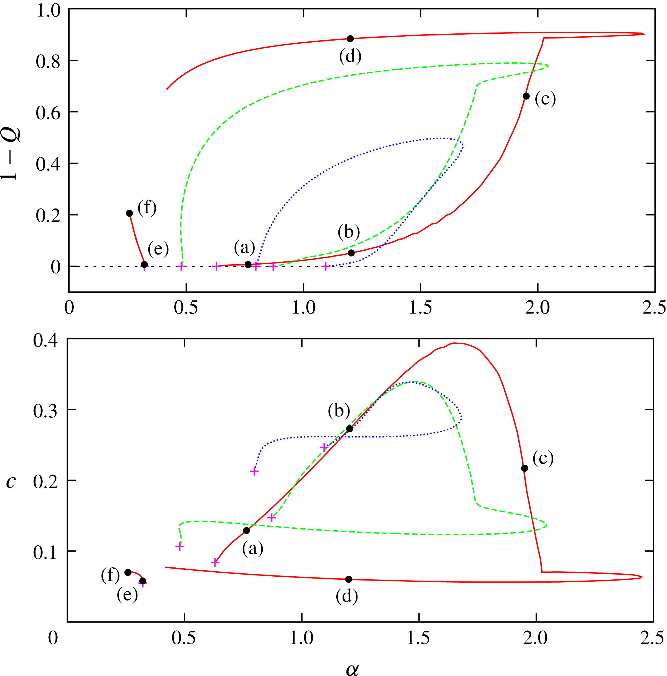
The bifurcation diagram of the Navier–Stokes solutions for PPF. Red (solid):
 $R=10^{6}$
. Green (dashed):
 $R=10^{5}$
. Blue (dotted):
 $R=10^{4}$
. The magenta crosses are the bifurcation points.

2 Governing equations, numerical method and finite Reynolds number results
Consider an unsteady two-dimensional incompressible fluid flow with dimensional velocity components
 $(u^{\ast },v^{\ast })$
between two walls placed at
 $y^{\ast }=\pm h^{\ast }$
in Cartesian coordinates
 $(x^{\ast },y^{\ast })$
. The flow is driven by a constant negative pressure gradient
 $-G^{\ast }$
in the direction of increasing
 $x^{\ast }$
. We denote the constant density and the kinematic viscosity of the fluid as
 $\unicode[STIX]{x1D70C}^{\ast }$
and
 $\unicode[STIX]{x1D708}^{\ast }$
, respectively. The unperturbed flow is the well-known parabolic profile
 $u^{\ast }=U^{\ast }\{1-(y^{\ast }/h^{\ast })^{2}\}$
, where
 $U^{\ast }=G^{\ast }h^{\ast 2}/2\unicode[STIX]{x1D70C}^{\ast }\unicode[STIX]{x1D708}^{\ast }$
is the centreline velocity. We seek a travelling wave propagating with the dimensional phase speed
 $c^{\ast }$
. This wave may generate a perturbation pressure
 $p^{\ast }$
, in addition to the constant gradient part. It is convenient to normalise the governing Navier–Stokes equations, by choosing the length and velocity scales as the channel half-width
 $h^{\ast }$
and
 $U^{\ast }$
, such that we can then introduce a non-dimensional velocity field
 $(u,v)=(u^{\ast },v^{\ast })/U^{\ast }$
, dependent on the dimensionless travelling wave coordinates
 $(x,y)=(x^{\ast }-c^{\ast }t^{\ast },y^{\ast })/h^{\ast }$
and the non-dimensional time
 $t=t^{\ast }U^{\ast }/h^{\ast }$
. The corresponding total pressure field is written as
 $(-G^{\ast }x^{\ast }+p^{\ast })/\unicode[STIX]{x1D70C}^{\ast }U^{\ast 2}=-2R^{-1}(x^{\ast }/h^{\ast })+p$
, where
 $p$
is the fluctuation part and
 $$\begin{eqnarray}\displaystyle & \displaystyle R=U^{\ast }h^{\ast }/\unicode[STIX]{x1D708}^{\ast }, & \displaystyle\end{eqnarray}$$
is the Reynolds number.
If we write the non-dimensional phase speed as
 $c=c^{\ast }/U^{\ast }$
, then the appropriate equations of motion are
 $$\begin{eqnarray}\displaystyle & \displaystyle (u-c)u_{x}+vu_{y}=2R^{-1}-p_{x}+R^{-1}\unicode[STIX]{x0394}u, & \displaystyle\end{eqnarray}$$
 $$\begin{eqnarray}\displaystyle & \displaystyle (u-c)v_{x}+vv_{y}=-p_{y}+R^{-1}\unicode[STIX]{x0394}v, & \displaystyle\end{eqnarray}$$
 $$\begin{eqnarray}\displaystyle & \displaystyle u_{x}+v_{y}=0, & \displaystyle\end{eqnarray}$$
where
 $\unicode[STIX]{x0394}=\unicode[STIX]{x2202}_{x}^{2}+\unicode[STIX]{x2202}_{y}^{2}$
throughout this section. The appropriate no-slip conditions are
 $$\begin{eqnarray}\displaystyle & \displaystyle u=v=0\quad \text{at}~y=\pm 1, & \displaystyle\end{eqnarray}$$
As a result the laminar basic Poiseuille flow acquires the non-dimensional form
 $$\begin{eqnarray}\displaystyle & \displaystyle u=u_{b}(y)\equiv 1-y^{2}. & \displaystyle\end{eqnarray}$$
We assume the velocities
 $[u,v](x,y)$
are periodic functions in
 $x$
with wavenumber
 $\unicode[STIX]{x1D6FC}$
. It is well known that the eigenfunction of a neutral TS wave has the symmetry
 $$\begin{eqnarray}\displaystyle & \displaystyle [u,v,p](x,y)=[u,-v,p](x+\unicode[STIX]{x03C0}/\unicode[STIX]{x1D6FC},-y). & \displaystyle\end{eqnarray}$$
We assume this symmetry throughout the paper, allowing us to subsequently focus our attention on just the lower half of the channel
 $y\in [-1,0]$
.
In order to simplify the problem, we decompose the flow field into its mean and fluctuation using the streamwise average
 $$\begin{eqnarray}\displaystyle & \displaystyle \overline{(\,\,\,)}=\frac{\unicode[STIX]{x1D6FC}}{2\unicode[STIX]{x03C0}}\int _{0}^{2\unicode[STIX]{x03C0}/\unicode[STIX]{x1D6FC}}(\,\,\,)\,\text{d}x. & \displaystyle\end{eqnarray}$$
Introducing a stream function
 $\unicode[STIX]{x1D713}$
for the fluctuation part, we let
 $u=\overline{u}+\unicode[STIX]{x1D713}_{y},v=-\unicode[STIX]{x1D713}_{x}$
, where
 $\overline{\unicode[STIX]{x1D713}}=\overline{p}=0$
. Then the continuity (2.2c
) is automatically satisfied, and we can write the fluctuation and mean parts of (2.2a,b
) in terms of the stream function as
 $$\begin{eqnarray}\displaystyle & \displaystyle (\overline{u}-c)\unicode[STIX]{x1D713}_{xy}-\overline{u}^{\prime }\unicode[STIX]{x1D713}_{x}+p_{x}=(\unicode[STIX]{x1D713}_{x}\unicode[STIX]{x1D713}_{yy}-\unicode[STIX]{x1D713}_{y}\unicode[STIX]{x1D713}_{xy})+R^{-1}\unicode[STIX]{x0394}\unicode[STIX]{x1D713}_{y}, & \displaystyle\end{eqnarray}$$
 $$\begin{eqnarray}\displaystyle & \displaystyle (\overline{u}-c)\unicode[STIX]{x1D713}_{xx}-p_{y}=(\unicode[STIX]{x1D713}_{x}\unicode[STIX]{x1D713}_{xy}-\unicode[STIX]{x1D713}_{y}\unicode[STIX]{x1D713}_{xx})+R^{-1}\unicode[STIX]{x0394}\unicode[STIX]{x1D713}_{x}, & \displaystyle\end{eqnarray}$$
 $$\begin{eqnarray}\displaystyle & \displaystyle -2R^{-1}=\overline{\unicode[STIX]{x1D713}_{x}\unicode[STIX]{x1D713}_{yy}}+R^{-1}\overline{u}^{\prime \prime }. & \displaystyle\end{eqnarray}$$
 $p$
can be eliminated by combining (2.6a
) and (2.6b
) to yield
 $$\begin{eqnarray}\displaystyle & \displaystyle (\overline{u}-c+\unicode[STIX]{x1D713}_{y})\unicode[STIX]{x0394}\unicode[STIX]{x1D713}_{x}-\unicode[STIX]{x1D713}_{x}(\overline{u}^{\prime \prime }+\unicode[STIX]{x0394}\unicode[STIX]{x1D713}_{y})=R^{-1}\unicode[STIX]{x0394}^{2}\unicode[STIX]{x1D713}. & \displaystyle\end{eqnarray}$$
Note that the boundary conditions and the symmetry property become
 $$\begin{eqnarray}\displaystyle & \displaystyle \unicode[STIX]{x1D713}=\unicode[STIX]{x1D713}_{y}=\overline{u}=0\quad \text{at}\,y=\pm 1, & \displaystyle\end{eqnarray}$$
and
 $$\begin{eqnarray}\displaystyle & \displaystyle [\overline{u},\unicode[STIX]{x1D713}](x,y)=[\overline{u},-\unicode[STIX]{x1D713}](x+\unicode[STIX]{x03C0}/\unicode[STIX]{x1D6FC},-y). & \displaystyle\end{eqnarray}$$
We can directly solve the Navier–Stokes equations (2.6c
) and (2.7) by a Chebyshev–Fourier spectral method. In order to determine the boundary conditions at the channel centre, we write
 $\unicode[STIX]{x1D713}=\unicode[STIX]{x1D713}^{(0)}+\unicode[STIX]{x1D713}^{(1)}$
, where
 $$\begin{eqnarray}\displaystyle & \displaystyle \unicode[STIX]{x1D713}^{(0)}(x,y)=\unicode[STIX]{x1D713}^{(0)}(x+\unicode[STIX]{x03C0}/\unicode[STIX]{x1D6FC},y),\quad \unicode[STIX]{x1D713}^{(1)}(x,y)=-\unicode[STIX]{x1D713}^{(1)}(x+\unicode[STIX]{x03C0}/\unicode[STIX]{x1D6FC},y), & \displaystyle\end{eqnarray}$$
respectively. Then from the symmetry (2.9) we see that
 $(\unicode[STIX]{x1D713}^{(0)},\unicode[STIX]{x1D713}^{(1)})$
must be (even, odd) functions in
 $y$
. Therefore, it follows that
 $$\begin{eqnarray}\displaystyle & \displaystyle \unicode[STIX]{x1D713}^{(0)}=\unicode[STIX]{x1D713}_{yy}^{(0)}=\unicode[STIX]{x1D713}_{y}^{(1)}=\unicode[STIX]{x1D713}_{yyy}^{(1)}=\overline{u}_{y}=0\quad \text{at}\,y=0. & \displaystyle\end{eqnarray}$$
The stream function and the mean flow are approximated by truncated Fourier–Chebyshev expansions of the form
 $$\begin{eqnarray}\displaystyle \unicode[STIX]{x1D713}=\left(\mathop{\sum }_{n=1}^{N}\mathop{\sum }_{l=0}^{L}s_{l,n}f_{l}^{(j)}(y)\text{e}^{\text{i}n\unicode[STIX]{x1D6FC}x}\right)+\text{c.c.},\quad \overline{u}=(1-y^{2})+\mathop{\sum }_{l=0}^{L}s_{l,0}g_{l}(y), & & \displaystyle\end{eqnarray}$$
where
 $j=(n\hspace{0.6em}{\rm mod}\hspace{0.2em}2)$
and the basis functions
 $[f_{l}^{(0)},f_{l}^{(1)},g_{l}]$
are
 $l$
th Chebyshev polynomials modified to satisfy the boundary conditions for
 $[\unicode[STIX]{x1D713}^{(0)},\unicode[STIX]{x1D713}^{(1)},\overline{u}]$
(see appendix A). In order to use Chebyshev polynomials over their usual domain,
 $y\in [-1,0]$
is mapped to
 $\unicode[STIX]{x1D702}\in [-1,1]$
. After substituting the expansions (2.12) into (2.6c
) and (2.7) and applying a Galerkin projection in
 $x$
, the equations are evaluated at the collocation points
 $\unicode[STIX]{x1D702}=\unicode[STIX]{x1D702}_{k}$
, where
 $$\begin{eqnarray}\displaystyle \unicode[STIX]{x1D702}_{k}=\cos \left(\frac{k+1}{L+2}\unicode[STIX]{x03C0}\right),\quad k=0,\ldots ,L, & & \displaystyle\end{eqnarray}$$
resulting in nonlinear algebraic equations for the
 $s_{l,n}$
which are solved by Newton’s iterative method.
The linearised version of (2.7) is the familiar Orr–Sommerfeld equation, and gives the neutral curve shown in figure 1. Near the neutral curve the initial seed of the Newton iteration can be chosen to be the linear solution. Once we have a solution at a point in
 $(\unicode[STIX]{x1D6FC},R)$
space, we can continue the solution branch by gradually changing either of these parameters. We define the non-dimensionalised flux
 $$\begin{eqnarray}\displaystyle Q=\left(\int _{-1}^{1}\overline{u}\,\text{d}y\right)\left(\int _{-1}^{1}u_{b}\,\text{d}y\right)^{-1} & & \displaystyle\end{eqnarray}$$
to provide an appropriate measure of the solution. Since finite-amplitude solutions typically have
 $Q<1$
, the quantity
 $1-Q$
can be viewed as a good indicator of the extent of nonlinearity.
The solution branches for Reynolds numbers
 $R=10^{4},10^{5},10^{6}$
, found in the manner described above, are summarised in figure 2. As shown by the branch for
 $R=10^{4}$
(the blue dotted curve), for
 $R>5772$
the bifurcation branch forms a loop that connects the two neutral points corresponding to the upper and lower neutral branches. For moderate Reynolds numbers the behaviour of the neutral surface in (amplitude,
 $\unicode[STIX]{x1D6FC}$
,
 $R$
) space is well understood, as can be seen for example in the computations by Herbert (Reference Herbert, Van de Vooren and Zandbergen1976) and Milinazzo & Saffman (Reference Milinazzo and Saffman1985). The solution branch bifurcates subcritically at the upper neutral branch, whilst the bifurcation is typically supercritical at the lower neutral branch (however, as we shall see later, for higher Reynolds numbers the bifurcation from the lower neutral branch becomes subcritical). Below the critical Reynolds number of
 $5772$
the solution curve is disconnected from the linear neutral curve and forms a closed loop, which exists down to
 $R\simeq 2939$
(see Herbert (Reference Herbert, Van de Vooren and Zandbergen1976), for example). Our moderate Reynolds number results are all consistent with the previous works. In the earlier works by Grohne (Reference Grohne1969), Chen & Joseph (Reference Chen and Joseph1973), Zahn et al. (Reference Zahn, Toomre, Spiegel and Gough1974), only a handful of Fourier modes were taken, although more recent works have increased the streamwise resolution. Here we use up to 340 Fourier modes together with a correspondingly large number of Chebyshev modes to reach larger Reynolds numbers than those studied by previous authors (see table 1).
The solution branch expands as
 $R$
is increased, and the associated flow typically involves small-scale structures due to the lack of significant diffusivity. Computation begins to become difficult when
 $R$
reaches
 $10^{6}$
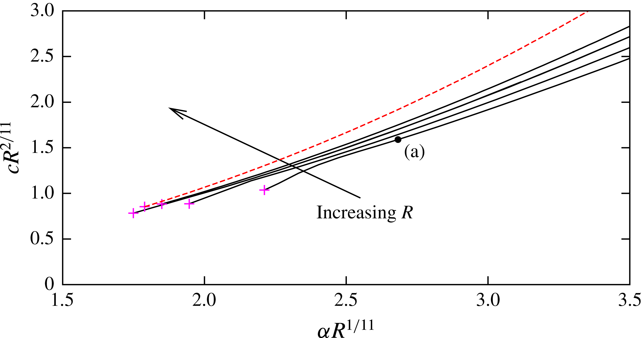
. To the authors’ best knowledge, this is the first time the Reynolds number of the travelling waves has been increased to this level. For this and larger Reynolds numbers the mapping method given in appendix A is used to accumulate the collocation points in the near-wall region, because here the structure is at its sharpest. Nevertheless, as shown by the red solid curve, we could not complete the loop at this value of Reynolds number due to the prohibitive computational expense and the ill-conditioned nature of the Jacobian matrix associated with the Newton iterations.
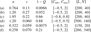
A summary of the properties of the solutions visualised in figure 3.


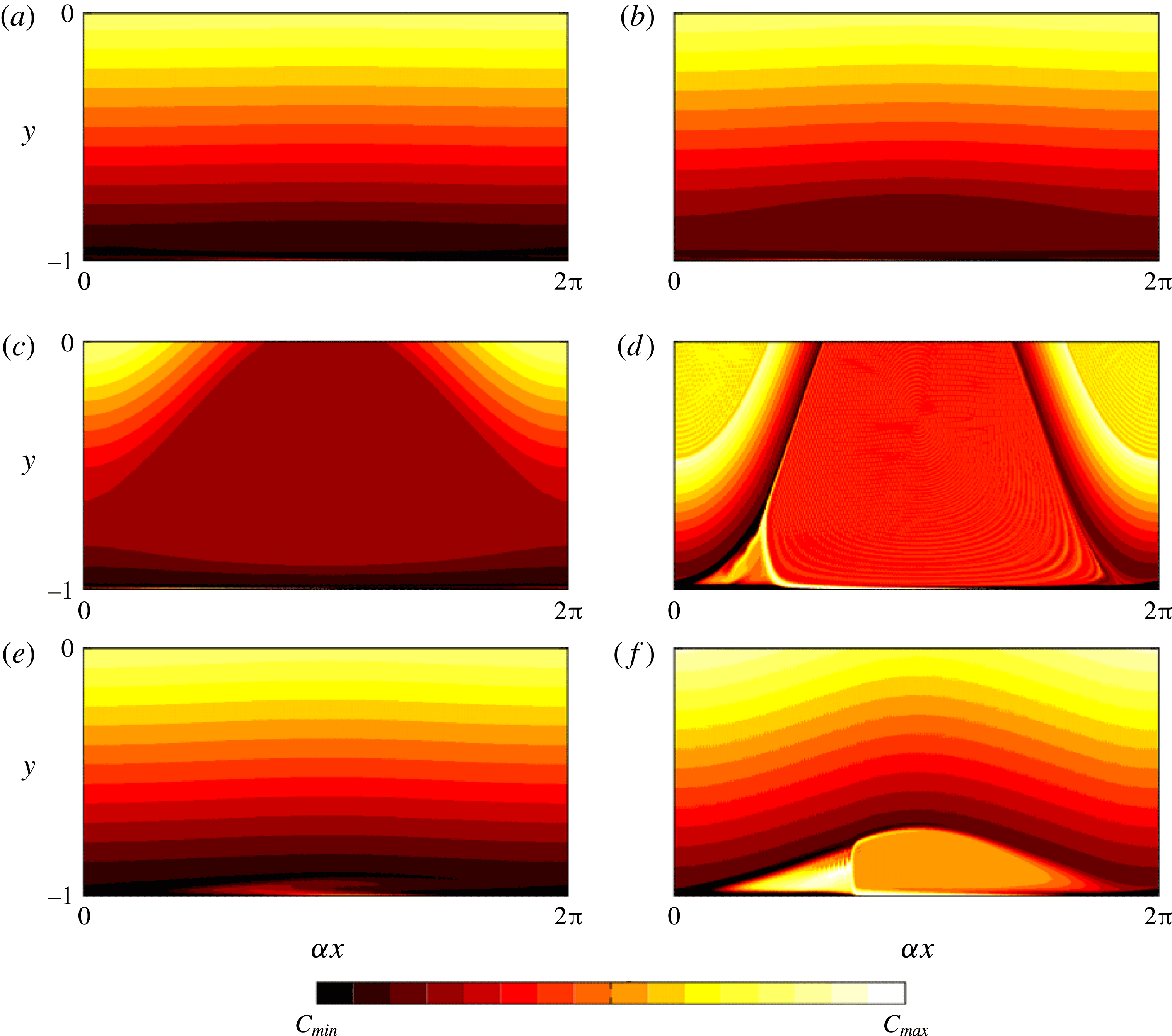
The difficulty appears to be due physically to the very sharp structure mentioned above no longer remaining confined to the near-wall zone. The development of the flow field along the bifurcation curve for
 $R=10^{6}$
is shown in figure 3. The contour plots (a)–(f) correspond to the points (a)–(f) shown in figure 2 and the key quantities associated with the solutions at these points are summarised in table 1. The total vorticity
 $$\begin{eqnarray}\displaystyle \unicode[STIX]{x1D714}=v_{x}-u_{y}=-\unicode[STIX]{x0394}\unicode[STIX]{x1D713}-\overline{u}^{\prime }, & & \displaystyle\end{eqnarray}$$
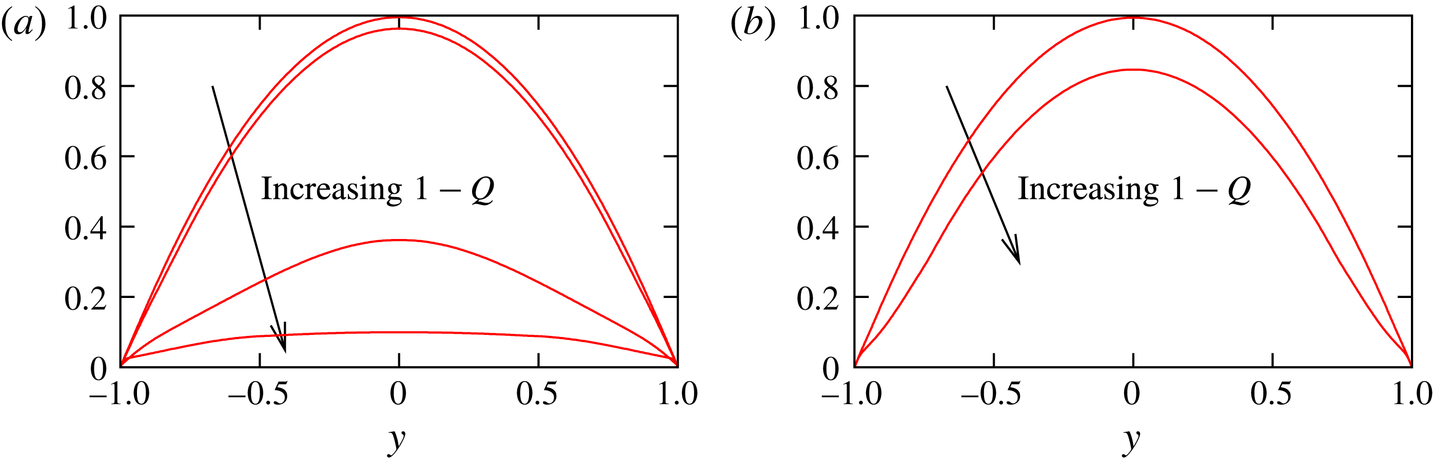
is chosen to visualise the flow fields in figure 3. From the upper-branch neutral point the solution branch bifurcates subcritically. The solution just after the bifurcation point is almost sinusoidal, as shown in (a). At this stage, the mean flow is very close to the parabolic basic flow profile, as can be seen in figure 4. Then, with increasing amplitude
 $(1-Q)$
, the flow eventually develops a constant vorticity region, as shown in figure 3(b). The region appears around the critical level
 $y=y_{c}$
, and possesses a familiar Kelvin’s cat’s eye shape. We shall see later that this uniform vorticity region is a consequence of the Prandtl–Batchelor theorem. The mean flow distortion remains small at this stage, as shown in figure 4, but is modified significantly once the solution branch reaches the point (c). The constant vorticity region has now expanded across the whole width of the channel, as shown in figure 3(c). It should be noted that up to this disturbance level the flow is almost symmetric in
 $x$
. This quasi symmetry is broken after the sudden turning point seen in the solution branch on figure 2. At location (d), a sharp structure appears at the perimeter of the constant vorticity region, and is apparently created by the separation of the near-wall flow structure. It seems that this separation is extremely effective in reducing the flow rate, as shown in the corresponding mean flow profile in figure 4. The solution that bifurcates from the lower-branch neutral curve develops in a similar way, but the structure remains concentrated near the wall. Just beyond the bifurcation point, as shown in figure 3(e), the flow structure throughout the majority of the flow is almost sinusoidal and, as expected, the mean flow distortion is small. Then, for larger amplitude, the disturbance near the wall develops a constant vorticity region, as shown in figure 3(f). The mean flow is distorted in the near-wall region, but it remains parabolic in the fluid core, as can be seen in figure 4(b).
3 General properties of Rayleigh’s equation and nonlinear critical layers
In the following sections we describe the various asymptotic theories relevant to the nonlinear solutions of PPF. Firstly however, we recall some general properties of Rayleigh’s equation
 $$\begin{eqnarray}\displaystyle & \displaystyle (\overline{u}-c)(\widehat{\unicode[STIX]{x1D713}}^{\prime \prime }-\unicode[STIX]{x1D6FC}^{2}\widehat{\unicode[STIX]{x1D713}})-\overline{u}^{\prime \prime }\widehat{\unicode[STIX]{x1D713}}=0, & \displaystyle\end{eqnarray}$$
and the analysis inside of the critical layer that occurs when
 $\overline{u}=c$
. Equation (3.1) can be derived from (2.7) by linearisation in
 $\unicode[STIX]{x1D713}$
, letting
 $R\rightarrow \infty$
and using a normal mode decomposition, so that to leading order
 $$\begin{eqnarray}\displaystyle & \displaystyle \unicode[STIX]{x1D713}=\frac{1}{2}\widehat{\unicode[STIX]{x1D713}}\text{e}^{\text{i}\unicode[STIX]{x1D6FC}x}+\text{c.c.},\quad \widehat{(\,\,\,)}={\displaystyle \frac{\unicode[STIX]{x1D6FC}}{\unicode[STIX]{x03C0}}}\int _{0}^{2\unicode[STIX]{x03C0}/\unicode[STIX]{x1D6FC}}(\,\,\,)\,\text{e}^{-\text{i}\unicode[STIX]{x1D6FC}x}\,\text{d}x. & \displaystyle\end{eqnarray}$$
For future purposes we also introduce the trigonometric form
 $$\begin{eqnarray}\displaystyle & \displaystyle \unicode[STIX]{x1D713}=\widehat{\unicode[STIX]{x1D713}}^{(e)}\cos (\unicode[STIX]{x1D6FC}x)+\widehat{\unicode[STIX]{x1D713}}^{(o)}\sin (\unicode[STIX]{x1D6FC}x),\quad \widehat{\unicode[STIX]{x1D713}}=\widehat{\unicode[STIX]{x1D713}}^{(e)}-\text{i}\widehat{\unicode[STIX]{x1D713}}^{(o)}. & \displaystyle\end{eqnarray}$$
Note that once
 $\widehat{\unicode[STIX]{x1D713}}$
is found from (3.1), the corresponding pressure field follows from the inviscid linear momentum equation as
 $$\begin{eqnarray}\displaystyle & \displaystyle \widehat{p}=\widehat{\unicode[STIX]{x1D713}}\,\overline{u}^{\prime }-(\overline{u}-c)\widehat{\unicode[STIX]{x1D713}}^{\prime }. & \displaystyle\end{eqnarray}$$
In the majority of this section we assume a fairly general background profile
 $\overline{u}(y)$
. However, we shall see in § 3.2 that the discussion there produces a consistent result only when the background flow is close to being inflectional at the critical position
 $y_{c}$
, or alternatively the amplitude of the wave is sufficiently large. Despite the fact that PPF is of course a non-inflectional profile, the discussion below is instructive in highlighting the underlying physics of the nonlinear development of the bifurcated nonlinear travelling waves. The asymptotic analysis for PPF is rather complicated and the reason for this is twofold. Firstly, the viscous nonlinear balance in the critical layer determines the jump in the phase of the wave across the layer and that information is indispensable in determining the neutral amplitude. Secondly, at large Reynolds number near the bifurcation point, the neutral wave possesses a long streamwise length scale (as can be seen in figure 1) which only reduces to an
 $O(1)$
value as the amplitude is increased into the strongly nonlinear regime. The second of these complications is completely excluded in this section, and that simplification allows us to focus only on the crucial effect of the phase shift on the outer Rayleigh structure. For PPF the underlying physics of the nonlinear wave remains similar, but occurs with more complicated vertical and streamwise scales.
Equation (3.1) becomes singular when
 $(\overline{u}-c)$
vanishes, because that factor is multiplied by the highest derivative. We write that critical position as
 $y=y_{c}$
. Using the method of Frobenius we can write the solution of (3.1) as a combination of two regular functions of
 $z=y-y_{c}$
,
 ${\mathcal{P}}_{a}(z)$
and
 ${\mathcal{P}}_{b}(z)$
as
 $$\begin{eqnarray}\displaystyle & \displaystyle \widehat{\unicode[STIX]{x1D713}}=a\,z\,{\mathcal{P}}_{a}(z)+b\,({\mathcal{P}}_{b}(z)+\unicode[STIX]{x1D707}_{c}z\ln |z|\,{\mathcal{P}}_{a}(z)), & \displaystyle\end{eqnarray}$$
 $$\begin{eqnarray}\displaystyle & \displaystyle {\mathcal{P}}_{a}(0)=1,\quad {\mathcal{P}}_{b}^{\prime }(0)=0, & \displaystyle\end{eqnarray}$$
where the constant
 $\unicode[STIX]{x1D707}_{c}$
is defined as the limit as
 $z\rightarrow 0$
of
 $$\begin{eqnarray}\displaystyle & \displaystyle \unicode[STIX]{x1D707}(z)=\frac{z\overline{u}^{\prime \prime }}{\overline{u}-c}. & \displaystyle\end{eqnarray}$$
The unknown complex constants
 $a,b$
are to be determined by the boundary conditions, but in general the values could differ for
 $z>0$
and
 $z<0$
. We can use an expansion of the form
 $\overline{u}-c=\unicode[STIX]{x1D706}_{1}z+\unicode[STIX]{x1D706}_{2}z^{2}+\cdots \,$
for small
 $z$
to show that
 $\unicode[STIX]{x1D707}_{c}=2\unicode[STIX]{x1D706}_{2}/\unicode[STIX]{x1D706}_{1}$
; here we assume
 $\unicode[STIX]{x1D706}_{1}>0$
. If the normalisation (3.6) holds, then the functions
 ${\mathcal{P}}_{a}(z)$
and
 ${\mathcal{P}}_{b}(z)$
are completely determined by solving the two regular equations
 $$\begin{eqnarray}\displaystyle & \displaystyle z{\mathcal{P}}_{a}^{\prime \prime }+2{\mathcal{P}}_{a}^{\prime }-(z\unicode[STIX]{x1D6FC}^{2}+\unicode[STIX]{x1D707}){\mathcal{P}}_{a}=0, & \displaystyle\end{eqnarray}$$
 $$\begin{eqnarray}\displaystyle & \displaystyle z{\mathcal{P}}_{b}^{\prime \prime }+\unicode[STIX]{x1D707}_{c}({\mathcal{P}}_{a}+2z{\mathcal{P}}_{a}^{\prime })-(z\unicode[STIX]{x1D6FC}^{2}+\unicode[STIX]{x1D707}){\mathcal{P}}_{b}=0, & \displaystyle\end{eqnarray}$$
 ${\mathcal{P}}_{a}(z)$
and
 ${\mathcal{P}}_{b}(z)$
have small-
 $z$
expansions of the form
 $$\begin{eqnarray}\displaystyle & \displaystyle {\mathcal{P}}_{a}=1+z\unicode[STIX]{x1D707}_{c}/2+O(z^{2}),\quad {\mathcal{P}}_{b}=1+O(z^{2}). & \displaystyle\end{eqnarray}$$
The jumps in
 $a,b$
across
 $z=0$
are found from a separate analysis in the critical layer, which is of thickness
 $\unicode[STIX]{x1D716}=R^{-1/3}$
, owing to the viscous-convective balance operating there. Here we further assume that nonlinearity influences the phase jump. This means that in the critical layer there is a balance between the viscous operator
 $R^{-1}\unicode[STIX]{x2202}_{y}^{2}\sim O(R^{-1}\unicode[STIX]{x1D716}^{-2})$
and the inertial operators
 $\overline{u}\unicode[STIX]{x2202}_{x}\sim O(\unicode[STIX]{x1D6FC}\unicode[STIX]{x1D716})$
and
 $v\unicode[STIX]{x2202}_{y}\sim O(\unicode[STIX]{x1D6FC}\unicode[STIX]{x1D713}/\unicode[STIX]{x1D716})$
. This balance, which is the source of the nonlinearity, reflects the fact that both the basic flow and the fluctuation stream function act as advective agents of equal importance. The balance is achieved if the size of
 $\unicode[STIX]{x1D713}$
is
 $O(\unicode[STIX]{x1D716}^{2})$
. We shall shortly see that
 $b$
is continuous across the critical layer but
 $a$
jumps by an imaginary constant. Therefore, reflecting the fact that
 $a,b\sim O(\unicode[STIX]{x1D716}^{2})$
, it is convenient to write
 $$\begin{eqnarray}\displaystyle & \displaystyle a=\unicode[STIX]{x1D716}^{2}(a_{0}+\text{i}\unicode[STIX]{x1D707}_{c}\unicode[STIX]{x1D6E9}),\quad b=\unicode[STIX]{x1D716}^{2}b_{0}, & \displaystyle\end{eqnarray}$$
where
 $$\begin{eqnarray}\displaystyle \unicode[STIX]{x1D6E9}=\left\{\begin{array}{@{}ll@{}}\unicode[STIX]{x1D6E9}_{0} & \text{if}\,z>0,\\ \unicode[STIX]{x1D6E9}_{0}+\unicode[STIX]{x1D703} & \text{if}\,z<0,\end{array}\right. & & \displaystyle\end{eqnarray}$$
and the quantity
 $\unicode[STIX]{x1D703}$
represents the aforementioned jump. Here
 $a_{0},\unicode[STIX]{x1D6E9}_{0},\unicode[STIX]{x1D703}$
are real constants, and without any loss of generality we can also set
 $b_{0}$
real with
 $b_{0}>0$
in (3.10) by suitably adjusting the phase of the wave. Then we can show from (3.3), (3.5) and (3.10) that the Rayleigh solution can be written as
 $$\begin{eqnarray}\displaystyle & \displaystyle \widehat{\unicode[STIX]{x1D713}}^{(e)}=\unicode[STIX]{x1D716}^{2}\{b_{0}{\mathcal{P}}_{b}(z)+a_{0}\,z{\mathcal{P}}_{a}(z)+b_{0}\unicode[STIX]{x1D707}_{c}z\ln |z|{\mathcal{P}}_{a}(z)\},\quad \widehat{\unicode[STIX]{x1D713}}^{(o)}=-\unicode[STIX]{x1D716}^{2}b_{0}\unicode[STIX]{x1D707}_{c}\unicode[STIX]{x1D6E9}z{\mathcal{P}}_{a}(z). & \displaystyle \nonumber\\ \displaystyle & & \displaystyle\end{eqnarray}$$
3.1 The nonlinear development of the critical layer
The singularity must be regularised by a thin critical layer surrounding
 $y=y_{c}$
. Inside the critical layer we expand
 $$\begin{eqnarray}\displaystyle & \displaystyle \overline{u}=c+\unicode[STIX]{x1D716}(\unicode[STIX]{x1D706}_{1}Z+w_{c})+\unicode[STIX]{x1D716}^{2}(\unicode[STIX]{x1D706}_{2}Z^{2}+W_{2}(Z))+\cdots \,, & \displaystyle\end{eqnarray}$$
 $$\begin{eqnarray}\displaystyle & \displaystyle \unicode[STIX]{x1D713}=\unicode[STIX]{x1D716}(\unicode[STIX]{x1D716}\unicode[STIX]{x1D719}_{1}(x,Z)+\cdots +\unicode[STIX]{x1D716}^{2}\unicode[STIX]{x1D719}_{2}(x,Z)+\cdots +\unicode[STIX]{x1D716}^{5}\unicode[STIX]{x1D719}_{5}(x,Z)+\cdots \,), & \displaystyle\end{eqnarray}$$
using
 $Z=\unicode[STIX]{x1D716}^{-1}(y-y_{c})$
. The first set of dots in (3.14) represents a term of order
 $\unicode[STIX]{x1D716}^{2}\ln \unicode[STIX]{x1D716}$
which matches to a logarithmic part of the outer Rayleigh solution: further analysis of this contribution is not necessary in the arguments that follow. The critical layer induces a core mean flow distortion
 $\unicode[STIX]{x1D716}w(y)$
where
 $w(y)$
is continuous with
 $w_{c}=w(y_{c})$
, but we allow for a discontinuity in its derivative and denote the derivatives just above and beneath the critical layer as
 $w_{c+}^{\prime }$
and
 $w_{c-}^{\prime }$
, respectively.
For what follows it is convenient to define the total stream functions
 $\unicode[STIX]{x1D6F7}_{1}$
and
 $\unicode[STIX]{x1D6F7}_{2}$
, so that
 $$\begin{eqnarray}\displaystyle & \displaystyle \unicode[STIX]{x1D6F7}_{1Z}=\unicode[STIX]{x1D719}_{1Z}+w_{c}+\unicode[STIX]{x1D706}_{1}Z,\quad \unicode[STIX]{x1D6F7}_{2Z}=\unicode[STIX]{x1D719}_{2Z}+W_{2}+\unicode[STIX]{x1D706}_{2}Z^{2}. & \displaystyle\end{eqnarray}$$
In view of (3.12) we require the following matching conditions as
 $Z\rightarrow \pm \infty$
:
 $$\begin{eqnarray}\displaystyle & \displaystyle \unicode[STIX]{x1D719}_{1}\rightarrow b_{0}\cos (\unicode[STIX]{x1D6FC}x), & \displaystyle\end{eqnarray}$$
and
 $$\begin{eqnarray}\displaystyle & \displaystyle \unicode[STIX]{x1D719}_{2}\rightarrow b_{0}\unicode[STIX]{x1D707}_{c}Z\{\ln |Z|\cos (\unicode[STIX]{x1D6FC}x)+J(\unicode[STIX]{x1D6FC}x)\}+a_{0}Z\cos (\unicode[STIX]{x1D6FC}x),\quad W_{2}\rightarrow w_{c\pm }^{\prime }Z, & \displaystyle\end{eqnarray}$$
where
 $$\begin{eqnarray}\displaystyle & \displaystyle J(\unicode[STIX]{x1D6FC}x)=-\unicode[STIX]{x1D6E9}\sin (\unicode[STIX]{x1D6FC}x)+\text{higher harmonics}. & \displaystyle\end{eqnarray}$$
An analysis inside of the critical layer reveals that
 $J$
is an odd function and experiences a jump across
 $y=y_{c}$
(see appendix B). At first sight it seems that the higher harmonics appearing in (3.18) contradict the leading-order monochromatic form for
 $\unicode[STIX]{x1D713}$
in the Rayleigh region (see (3.2)). However, provided the constant
 $\unicode[STIX]{x1D707}_{c}$
is asymptotically small (i.e.
 $\overline{u}$
is inflectional at the critical level to leading order), the higher harmonics play a negligible role outside of the critical layer (see also comments in § 3.2).
From the Navier–Stokes equations we find that the leading-order response is
 $$\begin{eqnarray}\displaystyle & \displaystyle (\unicode[STIX]{x1D6F7}_{1Z}\unicode[STIX]{x2202}_{x}-\unicode[STIX]{x1D6F7}_{1x}\unicode[STIX]{x2202}_{Z})\unicode[STIX]{x1D6F7}_{1ZZ}=\unicode[STIX]{x1D6F7}_{1ZZZZ}. & \displaystyle\end{eqnarray}$$
Despite the nonlinearity of this equation, a simple exact solution is possible, namely
 $$\begin{eqnarray}\displaystyle & \displaystyle \unicode[STIX]{x1D6F7}_{1}=\frac{\unicode[STIX]{x1D706}_{1}}{2}\left(Z+\frac{w_{c}}{\unicode[STIX]{x1D706}_{1}}\right)^{2}+b_{0}\cos (\unicode[STIX]{x1D6FC}x), & \displaystyle\end{eqnarray}$$
which ensures the continuity of
 $b_{0}$
across the critical layer and provides the key to unlocking the behaviour at higher orders. Also it is important to note here that there is virtually no effect of viscosity at this order because if we differentiate (3.20) four times with respect to
 $Z$
it vanishes identically. Hence the next-order response
 $$\begin{eqnarray}\displaystyle (\unicode[STIX]{x1D6F7}_{1Z}\unicode[STIX]{x2202}_{x}-\unicode[STIX]{x1D6F7}_{1x}\unicode[STIX]{x2202}_{Z})\unicode[STIX]{x1D6F7}_{2ZZ}=\unicode[STIX]{x1D6F7}_{2ZZZZ} & & \displaystyle\end{eqnarray}$$
determines the phase jump. The rescaling
 $\widetilde{Z}=(\unicode[STIX]{x1D706}_{1}/b_{0})^{1/2}(Z+w_{c}/\unicode[STIX]{x1D706}_{1})$
,
 $\unicode[STIX]{x1D709}=\unicode[STIX]{x1D6FC}x$
,
 $\unicode[STIX]{x1D6F7}=\unicode[STIX]{x1D6F7}_{2}(\unicode[STIX]{x1D706}_{1}/b_{0})^{3/2}/2\unicode[STIX]{x1D706}_{2}$
converts this problem to the simplified form
 $$\begin{eqnarray}\displaystyle & \displaystyle (\widetilde{Z}\unicode[STIX]{x2202}_{\unicode[STIX]{x1D709}}+\sin \unicode[STIX]{x1D709}\unicode[STIX]{x2202}_{\widetilde{Z}})\unicode[STIX]{x1D6F7}_{\widetilde{Z}\widetilde{Z}}=\unicode[STIX]{x1D6FE}\unicode[STIX]{x1D6F7}_{\widetilde{Z}\widetilde{Z}\widetilde{Z}\widetilde{Z}}, & \displaystyle\end{eqnarray}$$
where
 $\unicode[STIX]{x1D6FE}=(\unicode[STIX]{x1D706}_{1}/b_{0})^{1/2}/(\unicode[STIX]{x1D6FC}b_{0})$
is a measure of inverse amplitude. It can then be shown that the appropriate matching conditions to the Rayleigh solution are
 $$\begin{eqnarray}\displaystyle & \displaystyle \unicode[STIX]{x1D6F7}\sim \frac{\widetilde{Z}^{3}}{6}-\frac{\unicode[STIX]{x1D6E9}}{4\unicode[STIX]{x1D6FE}}\widetilde{Z}^{2}+\widetilde{Z}\{(\ln |\widetilde{Z}|+\text{const.})\cos \unicode[STIX]{x1D709}+J(\unicode[STIX]{x1D709})\},\quad \widetilde{Z}\rightarrow \pm \infty , & \displaystyle\end{eqnarray}$$
where the first term is due to the basic flow and the third term arises from the logarithmic singularity in the Rayleigh expansion (3.12). The second term is the shear jump in the mean flow distortion created by the interaction of the sinusoidal functions in (3.22) and (3.23). Haberman (Reference Haberman1972) solved the above problem and found the phase shift
 $\unicode[STIX]{x1D703}$
as a function of
 $\unicode[STIX]{x1D6FE}$
, whilst the fact that
 $J$
also contains higher harmonics was first recorded by Smith & Bodonyi (Reference Smith and Bodonyi1982a
) (see appendix B). In particular, both sets of authors found that
 $$\begin{eqnarray}\displaystyle \unicode[STIX]{x1D703}\rightarrow 0\quad \text{as}\,\unicode[STIX]{x1D6FE}\rightarrow 0, & & \displaystyle\end{eqnarray}$$
 $$\begin{eqnarray}\displaystyle \unicode[STIX]{x1D703}\rightarrow -\unicode[STIX]{x03C0}\quad \text{as}\,\unicode[STIX]{x1D6FE}\rightarrow \infty , & & \displaystyle\end{eqnarray}$$
with the latter result indicating that the phase shift approaches the classical value of
 $-\unicode[STIX]{x03C0}$
(see appendix B) as we revert back to the linear regime.
3.2 The non-existence of very small-amplitude states in PPF at order one wavenumbers
Now let us consider the physical significance of the phase shift
 $\unicode[STIX]{x1D703}$
for the behaviour outside of the critical layer, and the implication of it for PPF. The unperturbed flow has
 $\overline{u}=1-y^{2}$
, with
 $$\begin{eqnarray}\displaystyle \unicode[STIX]{x1D706}_{1}=-2y_{c},\quad \unicode[STIX]{x1D706}_{2}=-1,\quad y_{c}=-\sqrt{1-c}. & & \displaystyle\end{eqnarray}$$
In addition the symmetry condition
 $\widehat{\unicode[STIX]{x1D713}}^{\prime }=0$
at
 $y=0$
, and the impermeability condition
 $\widehat{\unicode[STIX]{x1D713}}=0$
at
 $y=-1$
should be applied to (3.1).
Two important features of the Rayleigh solution should be noted:
(i) If
 $y_{c}\notin [y_{1},y_{2}]$
, then the Wronskian of any two independent solutions of (3.1), say
 $\widehat{\unicode[STIX]{x1D713}}_{1},\widehat{\unicode[STIX]{x1D713}}_{2}$
, must satisfy
 $$\begin{eqnarray}\displaystyle & \displaystyle [\widehat{\unicode[STIX]{x1D713}}_{1}\widehat{\unicode[STIX]{x1D713}}_{2y}-\widehat{\unicode[STIX]{x1D713}}_{1y}\widehat{\unicode[STIX]{x1D713}}_{2}]_{y=y_{1}}^{y_{2}}=0. & \displaystyle\end{eqnarray}$$
(ii) Rayleigh solutions do not force the mean flow via a Reynolds stress: it is easy to see this by applying the fact that
 $\widehat{\unicode[STIX]{x1D713}}_{yy}$
is proportional to a real function of
 $y$
multiplied by
 $\widehat{\unicode[STIX]{x1D713}}$
in (2.6c
), and hence the Reynolds stress
 $(\text{i}\unicode[STIX]{x1D6FC}\widehat{\unicode[STIX]{x1D713}}\widehat{\unicode[STIX]{x1D713}}_{yy}^{\ast }+\text{c.c.})$
is identically zero.
The Frobenius solution suggests that if
 $\unicode[STIX]{x1D707}_{c}\unicode[STIX]{x1D703}\neq 0$
then across the critical layer the phase of the wave will jump. Here we remark that inviscid equations preserve symmetry in
 $x$
: for example, the Euler equations are invariant under reflection in
 $x$
but the Navier–Stokes equations are not. Therefore, the origin of this phase jump is the effect of viscosity within the critical layer. We further note that since
 $\widehat{\unicode[STIX]{x1D713}}^{(e)}$
and
 $\widehat{\unicode[STIX]{x1D713}}^{(o)}$
are two independent solutions of (3.1), then from the property (i) mentioned above,
 $$\begin{eqnarray}\displaystyle & \displaystyle 0=[\widehat{\unicode[STIX]{x1D713}}_{y}^{(e)}\widehat{\unicode[STIX]{x1D713}}^{(o)}-\widehat{\unicode[STIX]{x1D713}}^{(e)}\widehat{\unicode[STIX]{x1D713}}_{y}^{(o)}]_{y=y_{c+}}^{0}+[\widehat{\unicode[STIX]{x1D713}}_{y}^{(e)}\widehat{\unicode[STIX]{x1D713}}^{(o)}-\widehat{\unicode[STIX]{x1D713}}^{(e)}\widehat{\unicode[STIX]{x1D713}}_{y}^{(o)}]_{y=-1}^{y_{c-}}. & \displaystyle\end{eqnarray}$$
If we apply the symmetry condition (i.e.
 $\widehat{\unicode[STIX]{x1D713}}^{(e)}=\widehat{\unicode[STIX]{x1D713}}_{y}^{(o)}=0$
at
 $y=0$
, and thus we require
 $\unicode[STIX]{x1D6E9}_{0}=0$
) and the impermeability condition for
 $\widehat{\unicode[STIX]{x1D713}}^{(e)}$
(i.e.
 $\widehat{\unicode[STIX]{x1D713}}^{(e)}=0$
at
 $y=-1$
), (3.28) reduces to
 $$\begin{eqnarray}\displaystyle & \displaystyle [\widehat{\unicode[STIX]{x1D713}}^{(e)}\widehat{\unicode[STIX]{x1D713}}_{y}^{(o)}]_{y=y_{c-}}^{y_{c+}}=(\widehat{\unicode[STIX]{x1D713}}_{y}^{(e)}\widehat{\unicode[STIX]{x1D713}}^{(o)})|_{y=-1}. & \displaystyle\end{eqnarray}$$
Now it is easy to see that the left-hand side equals
 $b^{2}\unicode[STIX]{x1D707}_{c}\unicode[STIX]{x1D703}$
, and thus if this quantity is
 $O(1)$
the impermeability condition for
 $\widehat{\unicode[STIX]{x1D713}}^{(o)}$
cannot be satisfied. Of course, if the basic flow is inflectional in the vicinity of the critical level, then
 $\unicode[STIX]{x1D707}_{c}$
is zero to leading order, and there is no difficulty. However, for the linear PPF case
 $\unicode[STIX]{x1D703}\unicode[STIX]{x1D707}_{c}=-\unicode[STIX]{x03C0}/y_{c}$
, and it therefore follows that the critical layer solution is incompatible with the outer Rayleigh region. Therefore, it appears at first sight that there can be no large-Reynolds-number linear neutral solution for this flow.
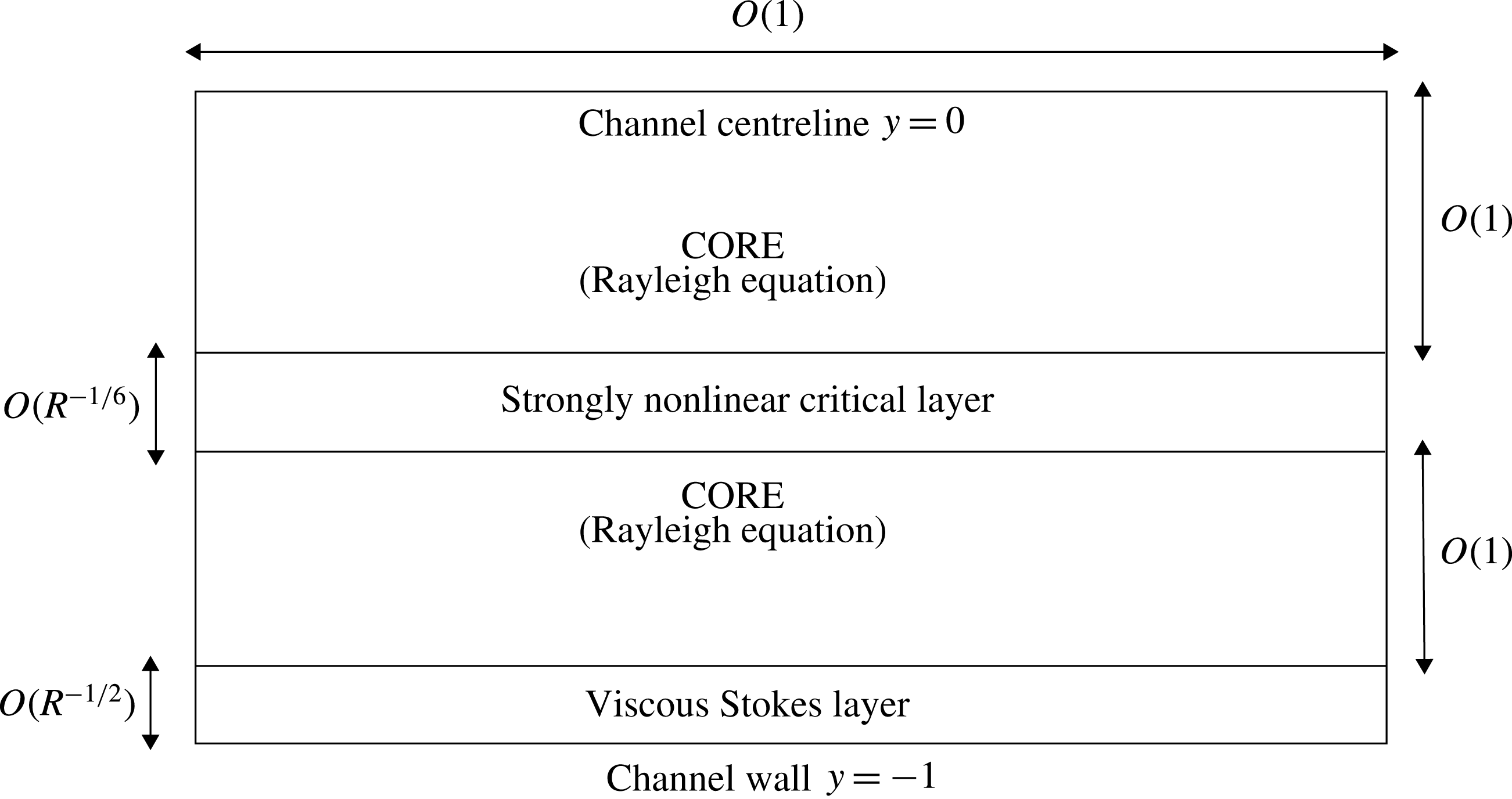
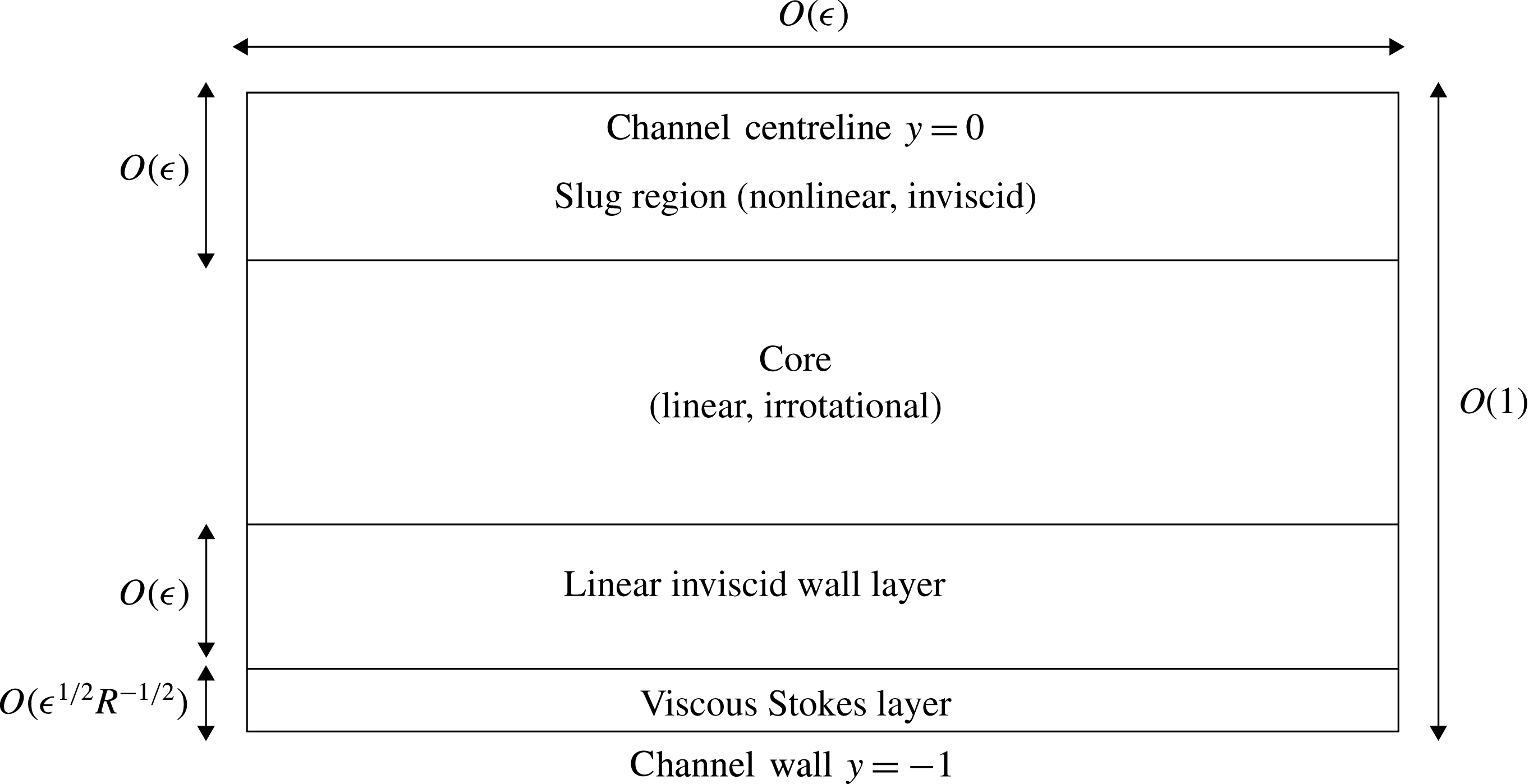
Nevertheless, such a structure is still possible provided the critical layer is situated sufficiently close to the wall, as we shall see in detail in the following sections. For the simplest case the critical layer is embedded within a viscous wall layer and the balance (3.29) is no longer relevant. This case corresponds to the lower neutral branch (see figure 5). Even when the critical layer is slightly detached from the wall, neutral solutions can still exist provided the ratio
 $b/a$
in a near-wall version of the Rayleigh solution is small. In this case the non-zero odd contribution to the stream function, induced by the jump across the critical layer, is small (see (3.29) and note that the size of the right-hand side is of the order of
 $ab$
). A small non-zero vertical velocity near the wall generated by the jump can now be reduced to zero within a thin Stokes layer attached to the wall which satisfies no-slip conditions (a sketch of the layer is given later in figure 10). This structure corresponds to a mode on the upper neutral branch, and the nonlinear development of the wave within the thin wall layer is similar to the one discussed here. Notably the structure of the critical layer remains identical near the bifurcation point. However, the associated matched asymptotic expansion becomes more complicated because of the long wavelength that is then in operation.
For larger amplitudes the modulus of the phase shift
 $|\unicode[STIX]{x1D703}|$
is expected to be asymptotically small, in view of (3.24), and a neutral Rayleigh structure is possible even for PPF (see the sketch later in figure 11). The physical reason for the vanishingly small phase shift is of course that now the convective terms completely dominate the higher-order critical layer structure (3.22): see the discussion just above (3.28) concerning the symmetry that appears in inviscid flows. In this strongly nonlinear case the phase shift occurs at higher order (corresponding to
 $\unicode[STIX]{x1D719}_{5}$
in (3.14)) due to viscous effects. Despite its now tiny size the phase shift still remains important, as its balance with the Stokes layer phase shift through (3.29) determines the amplitude of the wave, as described in § 5.2.
4 Bifurcation from the lower neutral branch
4.1 Nonlinear double-deck theory
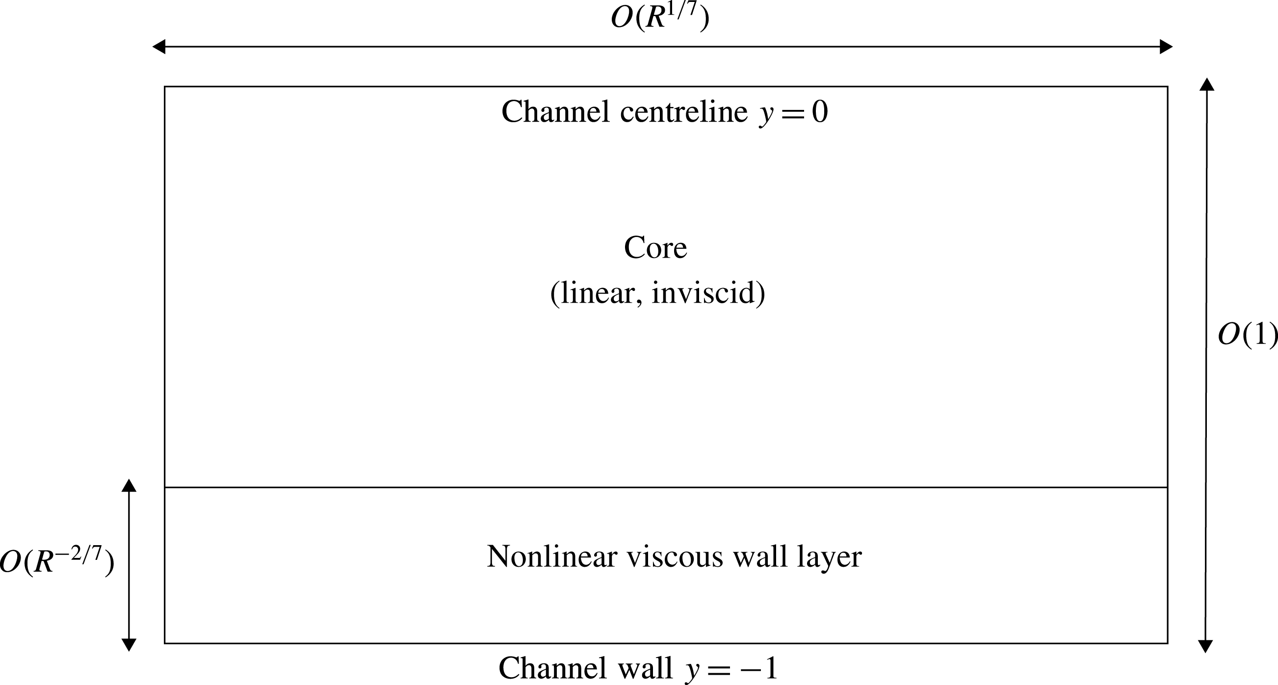
The nonlinear double-deck structure relevant for travelling wave solutions bifurcating from the lower branch of the linear neutral curve.

The lower-branch neutral wave is driven by near-wall dynamics, and in the majority of the flow field the fluid motion is predominantly inviscid. The wall layer (which is essentially a critical layer attached to the wall) is viscous and adjusts the inviscid flow appropriately in order to satisfy the no-slip condition. We shall see that, as the amplitude of the disturbance increases, nonlinear effects first become evident in the wall layer, whilst the core remains linear to leading order.
Let us estimate the thickness of the wall layer
 $\unicode[STIX]{x1D6FF}$
and the appropriate sizes of wavenumber and phase speed from an order of magnitude analysis. We denote the size of the stream function and pressure as
 $O(\unicode[STIX]{x1D713}),O(p)$
in the core and
 $O(\unicode[STIX]{x1D6F9}),O(P)$
, in the wall layer. Since the size of the stream function must be reduced towards the wall so that the normal velocity vanishes there,
 $O(\unicode[STIX]{x1D6F9})\sim O(\unicode[STIX]{x1D6FF}\unicode[STIX]{x1D713})$
. Then, in the wall layer, we require the terms on the left-hand side of (2.6a
) to be in balance. Thus,
 $$\begin{eqnarray}\displaystyle & \displaystyle O(\unicode[STIX]{x1D6FC}\unicode[STIX]{x1D6F9})\sim O(c\unicode[STIX]{x1D6FC}\unicode[STIX]{x1D6FF}^{-1}\unicode[STIX]{x1D6F9})\sim O(\unicode[STIX]{x1D6FC}P). & \displaystyle\end{eqnarray}$$
It should also be noted that the mean flow is
 $O(\unicode[STIX]{x1D6FF})$
in this layer. Next we examine the normal component of the momentum equation (2.6b
). In the wall layer the pressure gradient term dominates, indicating here that
 $P$
is independent of the vertical coordinate, and hence the order of magnitude of the pressure in the core and wall layer coincide, i.e.
 $O(p)\sim O(P)$
. However, in the core the pressure varies in
 $y$
, and thus the size of the convective term must be increased in order to balance the pressure term. That balance is achieved if
 $O(\unicode[STIX]{x1D6FC}^{2}\unicode[STIX]{x1D713})\sim O(p)$
, i.e.
 $O(\unicode[STIX]{x1D6FC}^{2}\unicode[STIX]{x1D6F9})\sim O(\unicode[STIX]{x1D6FF}P)$
. From this balance and (4.1), we have
 $$\begin{eqnarray}\displaystyle O(\unicode[STIX]{x1D6FC}^{2})\sim O(\unicode[STIX]{x1D6FF}),\quad O(c)\sim O(\unicode[STIX]{x1D6FF}),\quad O(P)\sim O(\unicode[STIX]{x1D6FF}^{2}). & & \displaystyle\end{eqnarray}$$
As we shall see in § 5, these balances also hold for the flow structure on the upper branch of the neutral curve. Returning to our investigation of the lower-branch structure, we wish to include the effects of both viscosity and nonlinearity within the wall layer. We therefore assume that the viscous term of
 $O(R^{-1}\unicode[STIX]{x1D6FF}^{-3}\unicode[STIX]{x1D6F9})$
is in balance with (4.1). This implies
 $\unicode[STIX]{x1D6FF}\sim (\unicode[STIX]{x1D6FC}R)^{-1/3}$
, from which the wall layer thickness can be determined to be
 $$\begin{eqnarray}\displaystyle & \displaystyle \unicode[STIX]{x1D6FF}=R^{-2/7}. & \displaystyle\end{eqnarray}$$
With the value of
 $\unicode[STIX]{x1D6FF}$
established, the orders of magnitude of all the other fluid quantities can be expressed in terms of
 $R$
. In particular we have
 $\unicode[STIX]{x1D6FC}\sim R^{-1/7},c\sim R^{-2/7},\unicode[STIX]{x1D6F9}\sim R^{-4/7}$
. A sketch of the asymptotic structure is given in figure 5.
Based on this order of magnitude analysis we now write
 $\unicode[STIX]{x1D6FC}_{0}=R^{1/7}\unicode[STIX]{x1D6FC}$
,
 $X=R^{-1/7}x$
and
 $c_{0}=R^{2/7}c$
in order to establish a formal asymptotic framework. We substitute the core expansions
 $$\begin{eqnarray}\displaystyle & \displaystyle \unicode[STIX]{x1D713}=\unicode[STIX]{x1D6FF}\unicode[STIX]{x1D713}_{0}(X,y)+\cdots \,,\quad p=\unicode[STIX]{x1D6FF}^{2}p_{0}(X,y)+\cdots & \displaystyle\end{eqnarray}$$
into (2.6a ) and (2.6b ), obtaining
 $$\begin{eqnarray}\displaystyle & \displaystyle u_{b}\unicode[STIX]{x1D713}_{0Xy}-u_{b}^{\prime }\unicode[STIX]{x1D713}_{0X}=0,\quad u_{b}\unicode[STIX]{x1D713}_{0XX}=p_{0y}, & \displaystyle\end{eqnarray}$$
which has solution
 $$\begin{eqnarray}\displaystyle & \displaystyle \unicode[STIX]{x1D713}_{0}=-Au_{b},\quad p_{0}=-A_{XX}\int ^{y}u_{b}^{2}\,\text{d}y_{\ast } & \displaystyle\end{eqnarray}$$
up to an unknown amplitude
 $A(X)$
, which satisfies
 $$\begin{eqnarray}\displaystyle & \displaystyle A(X)=-A(X+\unicode[STIX]{x03C0}/\unicode[STIX]{x1D6FC}), & \displaystyle\end{eqnarray}$$
in view of the assumed symmetry (2.9) and the evenness of
 $u_{b}$
in
 $y$
. Here we have used the fact that
 $\overline{u}_{0}=u_{b}(y)$
to leading order because the Reynolds stress acting on the leading part of
 $\overline{u}_{0}$
is determined solely by linear, inviscid fluctuations, and thus the property (ii) remarked upon in § 3.2 holds true here.
In the wall layer we expand
 $$\begin{eqnarray}\displaystyle & \displaystyle \unicode[STIX]{x1D713}=\unicode[STIX]{x1D6FF}^{2}\unicode[STIX]{x1D6F9}_{0}(X,Y)+\cdots \,,\quad \overline{u}=\unicode[STIX]{x1D6FF}\overline{U}_{0}(Y)+\cdots \,,\quad p=\unicode[STIX]{x1D6FF}^{2}P_{0}(X)+\cdots \,, & \displaystyle\end{eqnarray}$$
where
 $Y=\unicode[STIX]{x1D6FF}^{-1}(y+1)$
. Substituting these expansions into (2.6a
) and (2.6c
) we obtain the leading-order nonlinear problem
 $$\begin{eqnarray}\displaystyle & \displaystyle (\overline{U}_{0}-c_{0}+\unicode[STIX]{x1D6F9}_{0Y})\unicode[STIX]{x1D6F9}_{0XY}-(\overline{U}_{0}^{\prime }+\unicode[STIX]{x1D6F9}_{0YY})\unicode[STIX]{x1D6F9}_{0X}=-P_{0}^{\prime }+\unicode[STIX]{x1D6F9}_{0YYY}, & \displaystyle\end{eqnarray}$$
 $$\begin{eqnarray}\displaystyle & \displaystyle 0=\overline{\unicode[STIX]{x1D6F9}_{0X}\unicode[STIX]{x1D6F9}_{0YY}}+\overline{U}_{0}^{\prime \prime }. & \displaystyle\end{eqnarray}$$
 $$\begin{eqnarray}\displaystyle & \displaystyle \overline{U}_{0}=\unicode[STIX]{x1D6F9}_{0}=\unicode[STIX]{x1D6F9}_{0Y}=0,\quad \text{at}\,Y=0, & \displaystyle\end{eqnarray}$$
 $$\begin{eqnarray}\displaystyle & \displaystyle \overline{U}_{0}^{\prime }\rightarrow 2,\quad \unicode[STIX]{x1D6F9}_{0Y}\rightarrow -2A\quad \text{as}\,Y\rightarrow \infty . & \displaystyle\end{eqnarray}$$
 $P_{0}$
and the amplitude
 $A$
, using the core solution. First, the normal component of the momentum equation (2.6b
) reduces to
 $P_{0Y}=0$
, and thus in order to match to the core we require
 $P_{0}=p_{0}|_{y=-1}$
. Then using the symmetry (2.4) and the core solution (4.6) we have
 $$\begin{eqnarray}\displaystyle & \displaystyle P_{0}(X+\unicode[STIX]{x03C0}/\unicode[STIX]{x1D6FC}_{0})-P_{0}(X)=-{\textstyle \frac{16}{15}}A_{XX}. & \displaystyle\end{eqnarray}$$
In order to solve the nonlinear system (4.9)–(4.11) numerically, it is convenient to adopt the decomposition
 $\unicode[STIX]{x1D6F9}_{0}=\unicode[STIX]{x1D6F9}_{0}^{(1)}+\unicode[STIX]{x1D6F9}_{0}^{(0)}$
,
 $P_{0}=P_{0}^{(1)}+P_{0}^{(0)}$
with the same symmetries as in (2.10). Then from (4.10b
), (4.11):
 $$\begin{eqnarray}\displaystyle & \displaystyle P_{0X}^{(1)}=-{\textstyle \frac{4}{15}}\unicode[STIX]{x1D6F9}_{0XXXY}^{(1)}|_{Y\rightarrow \infty }, & \displaystyle\end{eqnarray}$$
whilst applying
 $\unicode[STIX]{x1D6F9}_{0Y}^{(0)}|_{Y\rightarrow \infty }=0$
to the far-field form of (4.9a
) we have
 $$\begin{eqnarray}\displaystyle & \displaystyle P_{0X}^{(0)}=(2\unicode[STIX]{x1D6F9}_{0X}^{(0)}-\unicode[STIX]{x1D6F9}_{0Y}^{(1)}\unicode[STIX]{x1D6F9}_{0XY}^{(1)})|_{Y\rightarrow \infty }. & \displaystyle\end{eqnarray}$$
Then we can eliminate
 $P_{0}$
and
 $A$
from the governing equations (4.9), (4.10) by substituting (4.12) and (4.13) into (4.9) and using the boundary conditions
 $$\begin{eqnarray}\displaystyle \overline{U}_{0}=\unicode[STIX]{x1D6F9}_{0}^{(0)}=\unicode[STIX]{x1D6F9}_{0Y}^{(0)}=\unicode[STIX]{x1D6F9}_{0}^{(1)}=\unicode[STIX]{x1D6F9}_{0Y}^{(1)}=0,\quad \text{at}\,Y=0, & & \displaystyle\end{eqnarray}$$
 $$\begin{eqnarray}\displaystyle \overline{U}_{0}^{\prime }\rightarrow 2,\quad \unicode[STIX]{x1D6F9}_{0Y}^{(0)}\rightarrow 0,\quad \unicode[STIX]{x1D6F9}_{0YY}^{(1)}\rightarrow 0\quad \text{as}\,Y\rightarrow \infty . & & \displaystyle\end{eqnarray}$$
In order to numerically solve this reduced system we expand
 $$\begin{eqnarray}\displaystyle & \displaystyle \unicode[STIX]{x1D6F9}_{0}=\left(\mathop{\sum }_{l=0}^{L}\mathop{\sum }_{n=1}^{N}s_{l,n}F_{l}^{(j)}(Y)\text{e}^{\text{i}n\unicode[STIX]{x1D6FC}_{0}X}\right)+\text{c.c.},\quad \overline{U}_{0}=2Y+\mathop{\sum }_{l=0}^{L}s_{l,0}G_{l}(Y), & \displaystyle\end{eqnarray}$$
where
 $j=(n\hspace{0.6em}{\rm mod}\hspace{0.2em}2)$
and
 $[F_{l}^{(0)},F_{l}^{(1)},G_{l}]$
are modified
 $l$
th Chebyshev polynomials defined in appendix A, satisfying boundary conditions for
 $[\unicode[STIX]{x1D6F9}_{0}^{(0)},\unicode[STIX]{x1D6F9}_{0}^{(1)},\overline{U}_{0}]$
. Newton’s method can be used to find the spectral coefficients
 $s_{l,n}$
in the same way as when solving the Navier–Stokes equations in § 2.
Before we describe the numerical results, we confirm that at small amplitude the asymptotic system yields the well-known lower-branch neutral point. Considering the wall layer problem (4.9)–(4.10) linearised around the basic flow and seeking a small-amplitude response of the normal mode form
 $$\begin{eqnarray}\displaystyle & \displaystyle \overline{U}_{0}=2Y,\quad (\unicode[STIX]{x1D6F9}_{0},P_{0},A)={\textstyle \frac{1}{2}}(\widehat{\unicode[STIX]{x1D6F9}}_{0}(\unicode[STIX]{x1D701}),\widehat{P}_{0},\widehat{A})\text{e}^{\text{i}\unicode[STIX]{x1D6FC}_{0}X}+\text{c.c.}, & \displaystyle\end{eqnarray}$$
where the new variable
 $\unicode[STIX]{x1D701}=(2\text{i}\unicode[STIX]{x1D6FC}_{0})^{1/3}(Y-c_{0}/2),$
we find that
 $\widehat{\unicode[STIX]{x1D6F9}}_{0}$
satisfies
 $$\begin{eqnarray}\displaystyle & \displaystyle \unicode[STIX]{x1D701}\widehat{\unicode[STIX]{x1D6F9}}_{0\unicode[STIX]{x1D701}}-\widehat{\unicode[STIX]{x1D6F9}}_{0}=-\widehat{P}_{0}/2+\widehat{\unicode[STIX]{x1D6F9}}_{0\unicode[STIX]{x1D701}\unicode[STIX]{x1D701}\unicode[STIX]{x1D701}}. & \displaystyle\end{eqnarray}$$
The boundary conditions on (4.17) are, from (4.10):
 $$\begin{eqnarray}\displaystyle & \displaystyle \widehat{\unicode[STIX]{x1D6F9}}_{0}(\unicode[STIX]{x1D701}_{0})=\widehat{\unicode[STIX]{x1D6F9}}_{0\unicode[STIX]{x1D701}}(\unicode[STIX]{x1D701}_{0})=0,\quad \widehat{\unicode[STIX]{x1D6F9}}_{0\unicode[STIX]{x1D701}}(\infty )=-2\widehat{A}/(2\text{i}\unicode[STIX]{x1D6FC}_{0})^{1/3}, & \displaystyle\end{eqnarray}$$
where
 $\unicode[STIX]{x1D701}_{0}=-(2\text{i}\unicode[STIX]{x1D6FC}_{0})^{1/3}c_{0}/2$
is the value of
 $\unicode[STIX]{x1D701}$
on the wall
 $Y=0.$
Noting that
 $\widehat{\unicode[STIX]{x1D6F9}}_{0\unicode[STIX]{x1D701}\unicode[STIX]{x1D701}}$
satisfies Airy’s equation, the linearised system (4.17), (4.18) may be integrated to yield
 $$\begin{eqnarray}\displaystyle & \displaystyle \widehat{\unicode[STIX]{x1D6F9}}_{0\unicode[STIX]{x1D701}}=\frac{2\widehat{A}}{(2\text{i}\unicode[STIX]{x1D6FC}_{0})^{1/3}}\left(\frac{\unicode[STIX]{x1D705}(\unicode[STIX]{x1D701})}{\unicode[STIX]{x1D705}(\unicode[STIX]{x1D701}_{0})}-1\right),\quad \unicode[STIX]{x1D705}(\unicode[STIX]{x1D701})=\int _{\unicode[STIX]{x1D701}}^{\infty }\text{Ai}(s)\,\text{d}s. & \displaystyle\end{eqnarray}$$
Evaluating (4.17) on the wall, and making use of (4.19), we have
 $$\begin{eqnarray}\displaystyle & \displaystyle \frac{\widehat{P}_{0}}{2}=-\frac{2\widehat{A}}{(2\text{i}\unicode[STIX]{x1D6FC}_{0})^{1/3}}\frac{\text{Ai}^{\prime }(\unicode[STIX]{x1D701}_{0})}{\unicode[STIX]{x1D705}(\unicode[STIX]{x1D701}_{0})}, & \displaystyle\end{eqnarray}$$
Using (4.6), the core flow can also be written in the normal mode form
 $$\begin{eqnarray}\displaystyle & \displaystyle \unicode[STIX]{x1D713}_{0}={\textstyle \frac{1}{2}}\widehat{\unicode[STIX]{x1D713}}_{0}(y)\text{e}^{\text{i}\unicode[STIX]{x1D6FC}_{0}X}+\text{c.c.},\quad \widehat{\unicode[STIX]{x1D713}}_{0}=-\widehat{A}u_{b}, & \displaystyle\end{eqnarray}$$
while, from the pressure–displacement law (4.11):
 $$\begin{eqnarray}\displaystyle & \displaystyle \widehat{P}_{0}=-{\textstyle \frac{8}{15}}\unicode[STIX]{x1D6FC}_{0}^{2}\widehat{A}. & \displaystyle\end{eqnarray}$$
Combining (4.20) and (4.22) we obtain the familiar lower-branch PPF dispersion relation
 $$\begin{eqnarray}\displaystyle & \displaystyle \unicode[STIX]{x1D6FC}_{0}^{7/3}=-\frac{15}{8}(2\text{i})^{5/3}\frac{\text{Ai}^{\prime }(\unicode[STIX]{x1D701}_{0})}{\unicode[STIX]{x1D705}(\unicode[STIX]{x1D701}_{0})}. & \displaystyle\end{eqnarray}$$
It is a straightforward numerical task to find the values of
 $\unicode[STIX]{x1D701}_{0},\unicode[STIX]{x1D6FC}_{0}$
from the real and imaginary parts of (4.23), and this yields the well-known result
 $(\unicode[STIX]{x1D6FC}_{0},c_{0})\approx (2.149,2.826)$
, shown as the lower asymptote on figure 1, which can be compared with that arising from previous linear analyses of PPF (for example, Reid Reference Reid and Holt1965).
4.2 Comparison of nonlinear lower-branch Navier–Stokes and asymptotic computations
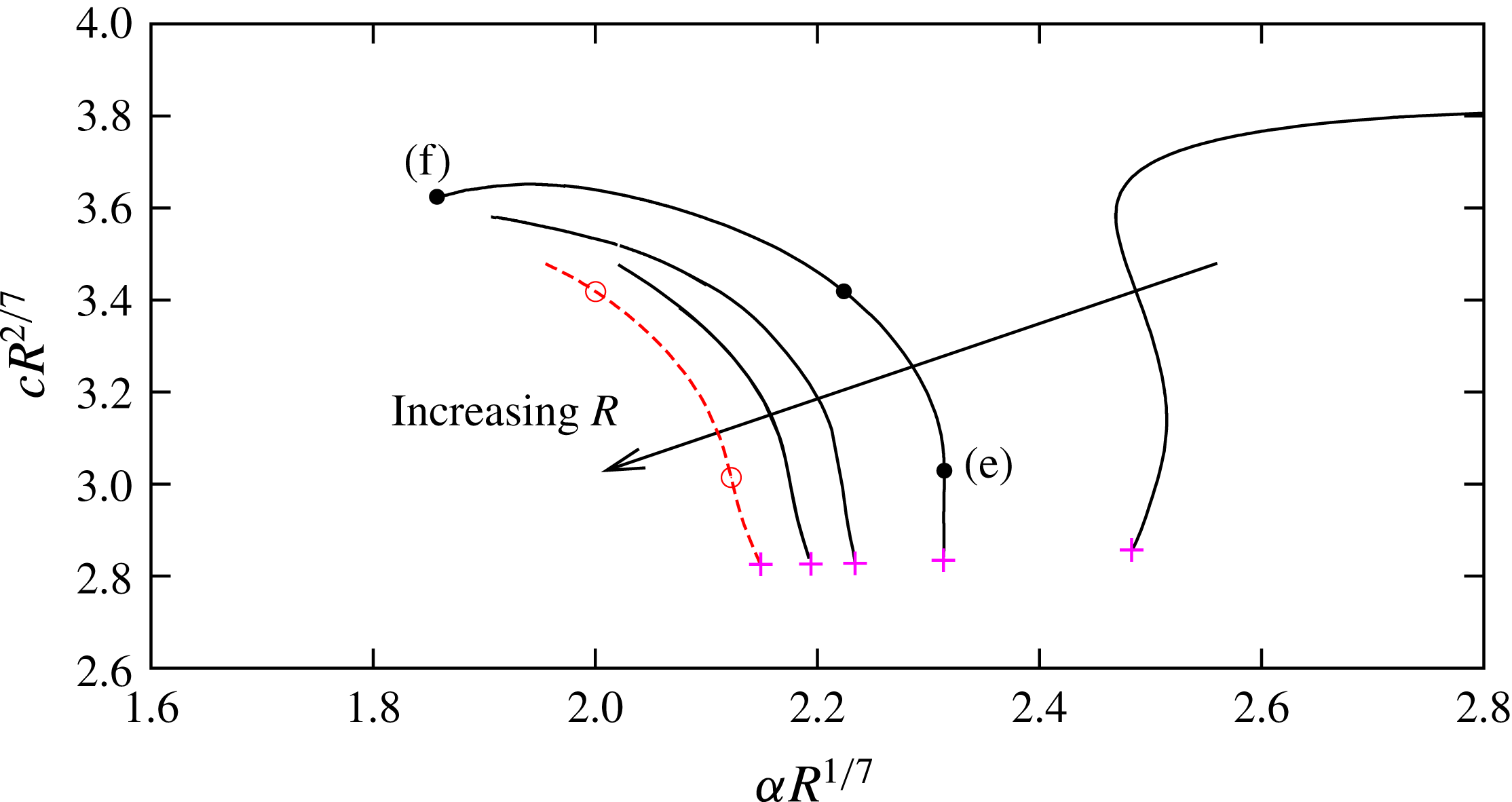
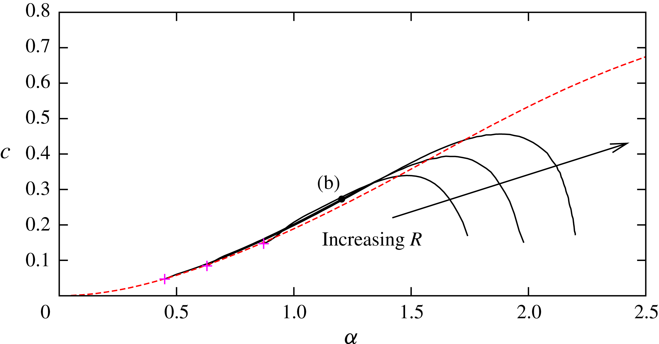
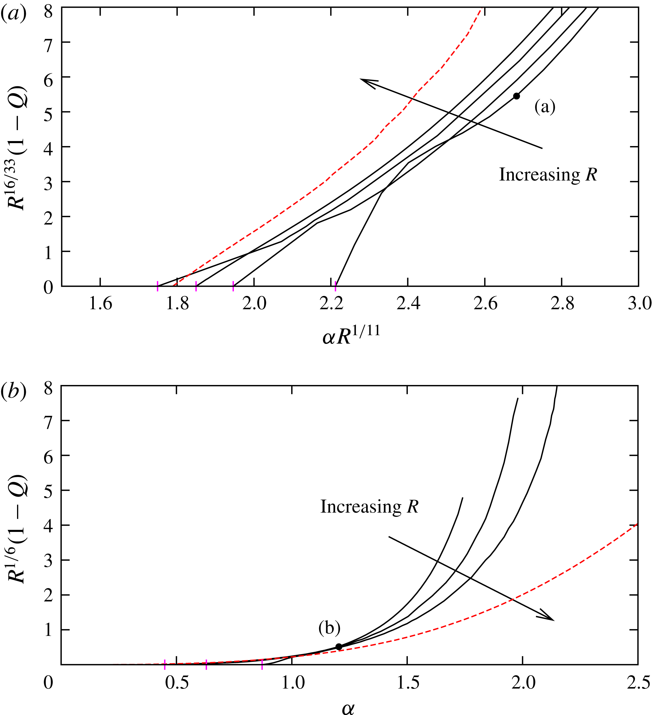
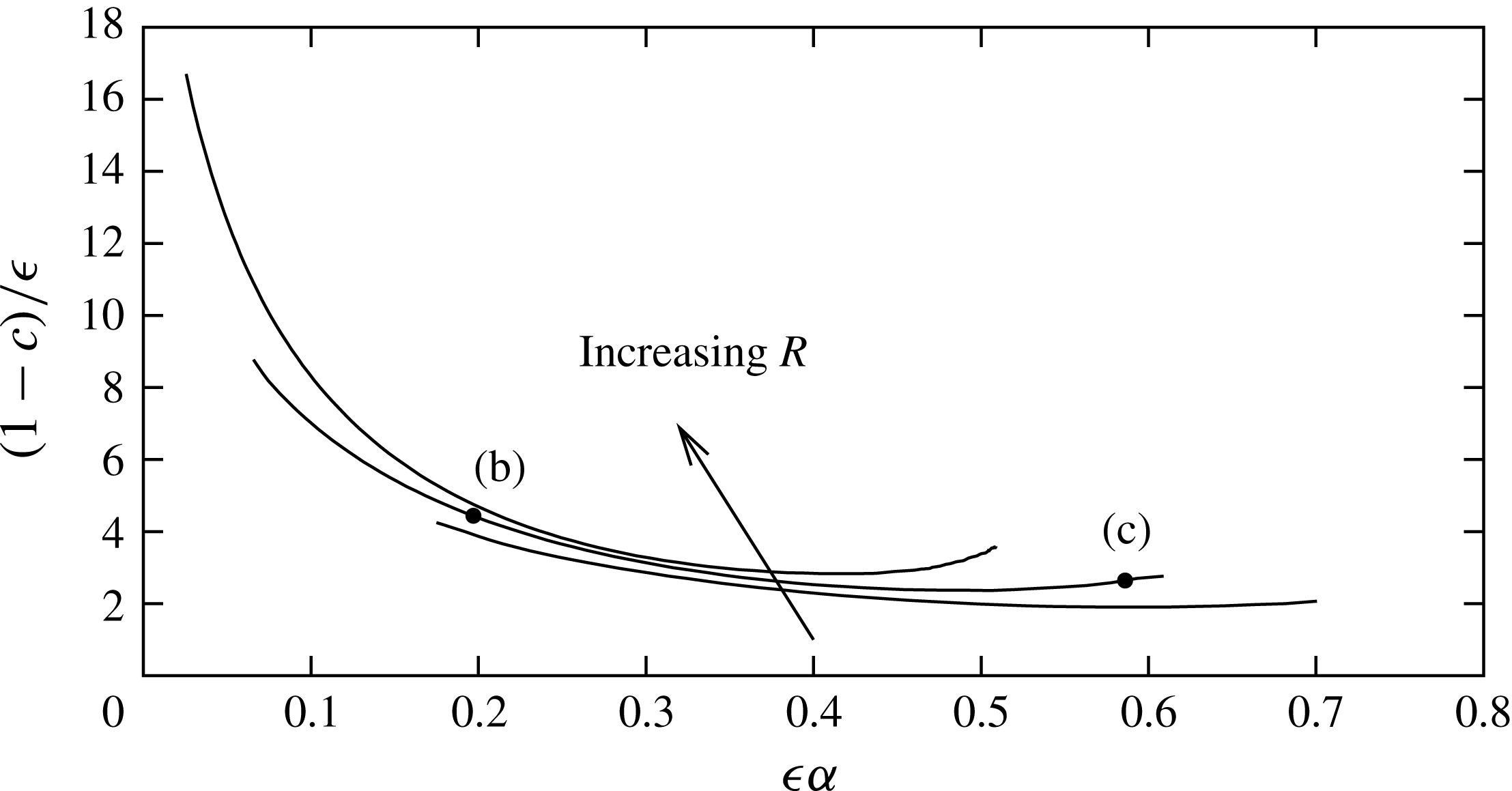
We first compare the bifurcation diagram obtained from the computation of the nonlinear lower-branch asymptotic problem (4.9), (4.12)–(4.14) with the Navier–Stokes results. Figure 6 shows the comparison of the solution curves on the lower-branch scale. We can see that at large Reynolds number the Navier–Stokes results converge to the asymptotic result shown by the red dashed curve. The bifurcation is supercritical for
 $R=10^{5}$
and
 $10^{6}$
, as Itoh (Reference Itoh1974) predicted from a weakly nonlinear analysis of the Navier–Stokes equations. However, our computations for
 $R$
larger than
 $10^{7}$
show that the nature of the bifurcation becomes supercritical when
 $R$
is sufficiently large. This is consistent with the large-Reynolds-number analysis of Hall & Smith (Reference Hall and Smith1982).
The point (e) corresponds to that in figure 2. At this point
 $cR^{2/7}=3$
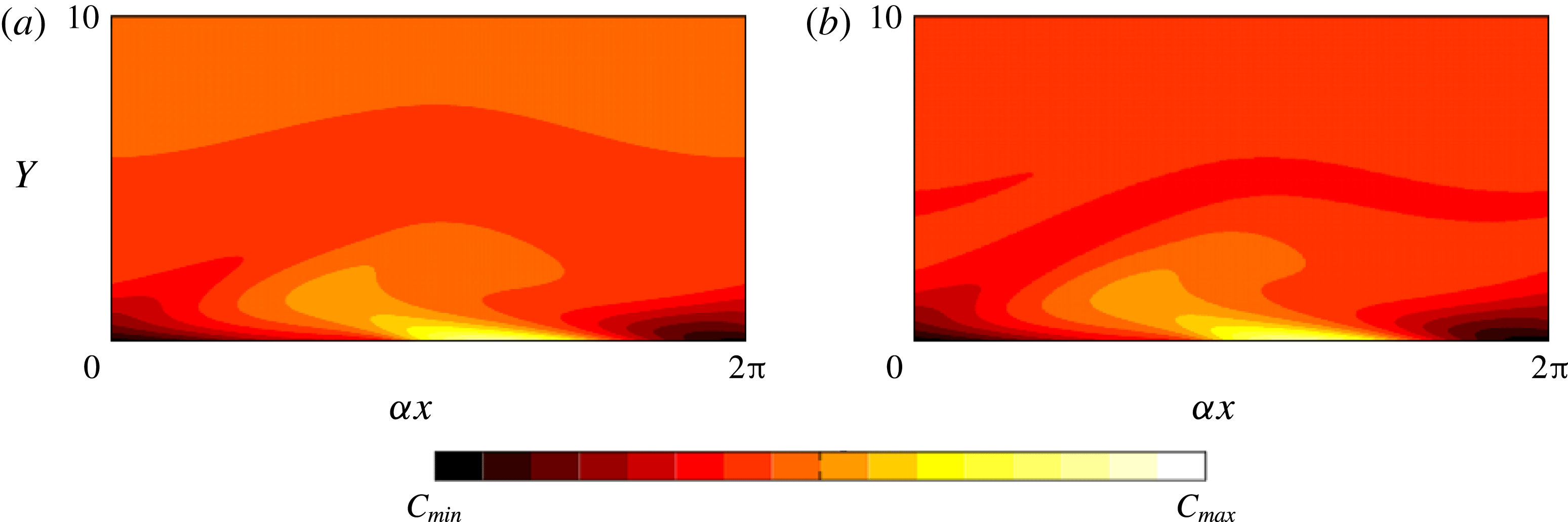
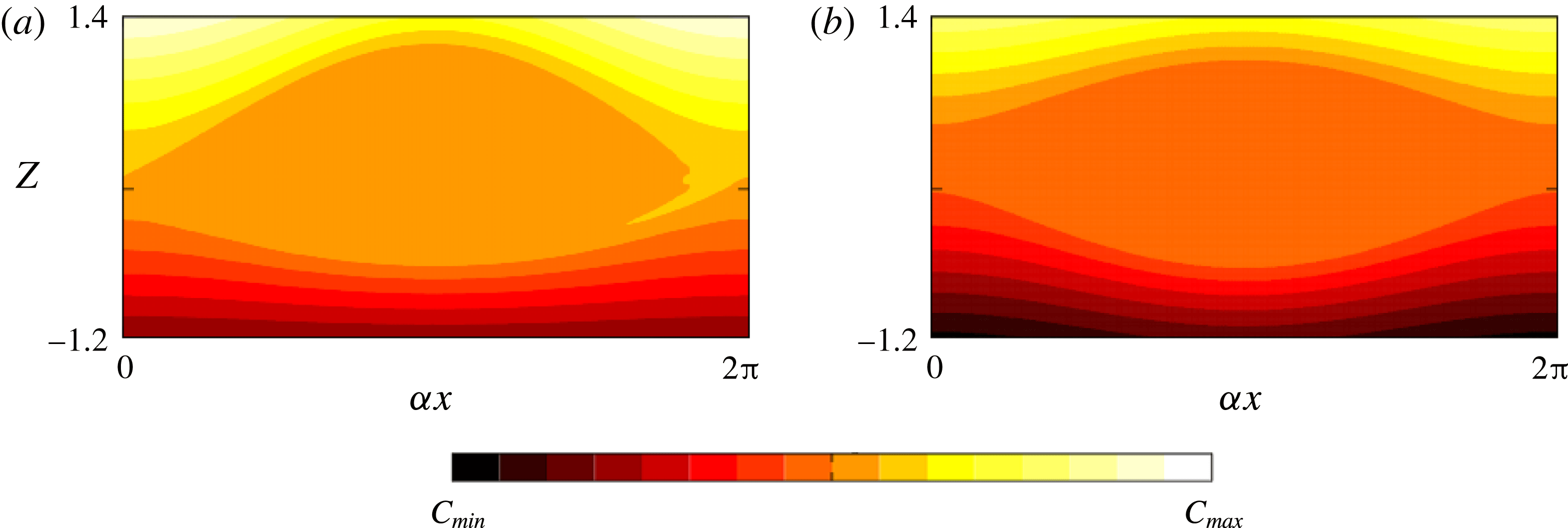
, and for this value of phase speed we compare the Navier–Stokes near-wall flow field to that found from the solution of the asymptotic problem. The comparison of the total vorticity, given in figure 7, shows excellent agreement. In the asymptotic result only the leading-order part is used, namely the terms in the curly bracket in the asymptotic expansion
 $$\begin{eqnarray}\displaystyle & \displaystyle \unicode[STIX]{x1D714}=\{-\unicode[STIX]{x1D6F9}_{0YY}-\overline{U}_{0Y}\}+\cdots \,. & \displaystyle\end{eqnarray}$$
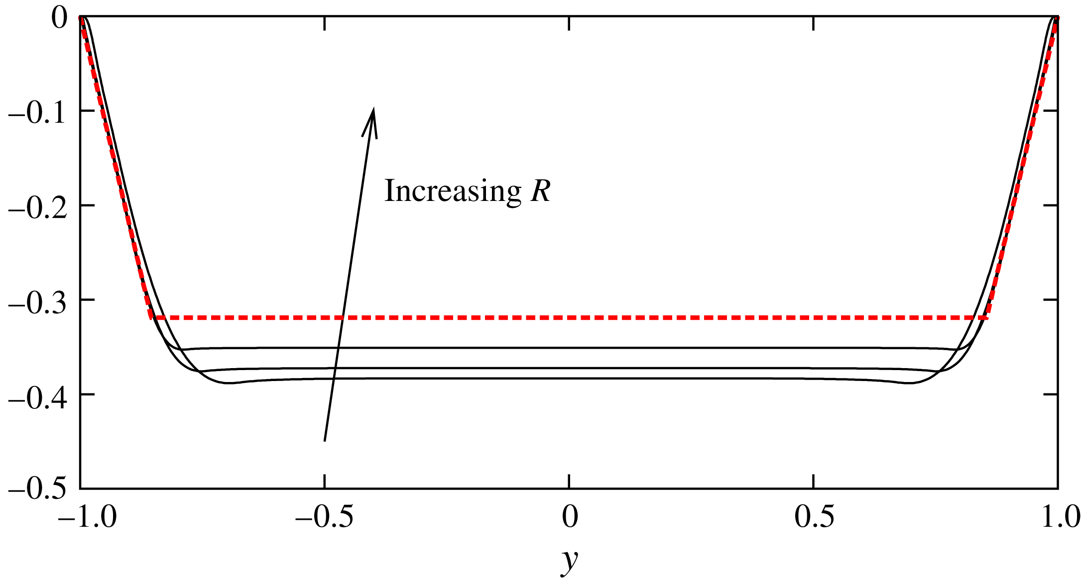
The convergence of the mean flow distortion is also confirmed at this phase speed (see figure 8).
At this disturbance level the flow field is slowly varying in the streamwise direction. However, further away from the bifurcation point (i.e. for larger
 $cR^{2/7}$
) the flow develops a sharp structure, as was shown earlier in figure 3(f). We can see how this structure emerges in figure 9: here we plot the wall shear
 $u_{y}(y=-1)$
versus
 $\unicode[STIX]{x1D6FC}x$
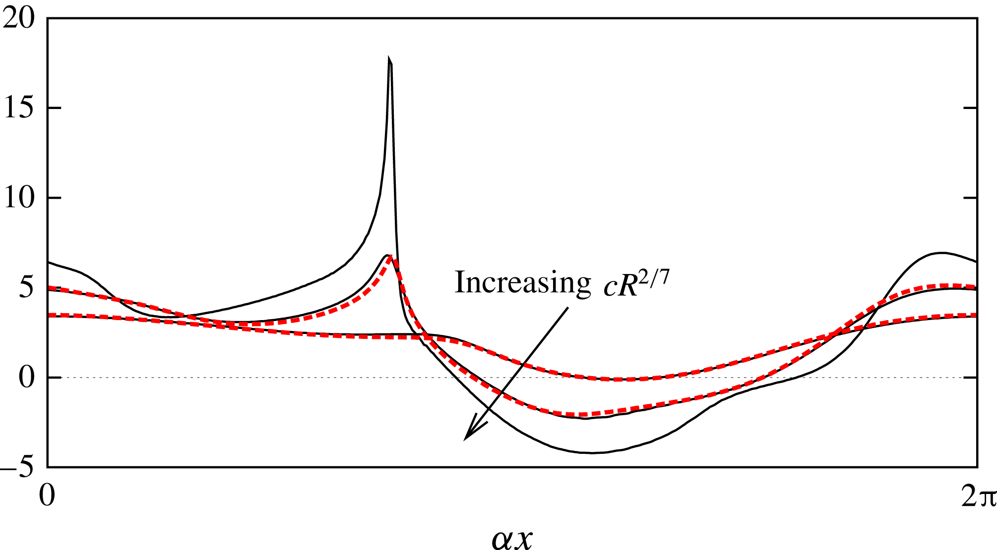
for the solutions denoted by the filled and open circles in figure 6. It should be noted that the wall shear stress calculated using the asymptotic theory passes through zero in a smooth fashion: this is to be expected since the lower branch equations (4.9)–(4.11) are elliptic in the streamwise direction due to the pressure–displacement law (4.11), and therefore no Goldstein singularity will arise. This phenomenon is similar to that observed in calculations of the interactive boundary layer flow over a surface roughness, where regular separation is encountered as the roughness height parameter approaches a critical value (see, for example, Smith & Walton Reference Smith and Walton1998). We can see from both the Navier–Stokes and asymptotic results that the flow is becoming localised: this seems to suggest that the asymptotic theory will eventually break down as it is based on an assumed slow streamwise development of the flow. The emergence of this sharp structure requires many Fourier modes to fully resolve, and it was not possible to continue the computation of either the Navier–Stokes or the asymptotic problem beyond the end point of the branch shown in figure 6. In a similar investigation of nonlinear lower-branch travelling waves, but in the context of boundary layer flow, Hall (Reference Hall1995) also reported an inability to continue the neutral branch beyond a critical amplitude. In that case the difficulty appeared to be associated with the wall shear approaching zero at a specific streamwise location, whereas in the present scenario, as noted above, we had no difficulty obtaining solutions with negative values of this quantity. In fact, according to figure 9, our localisation appears to be occurring in a region where the wall shear is strongly positive. The difference is likely to be caused by the different forms of the pressure–displacement law relevant to these two cases.
The bifurcation diagram on the lower-branch scale. The solid black curves are Navier–Stokes results for
 $R=10^{5},10^{6},10^{7},10^{8}$
. The points indicated by (e) and (f) are those seen in figure 2. The red dashed curve is the asymptotic result. The magenta crosses are the bifurcation points from the linear neutral curve.

The comparison of total vorticity in the wall layer for
 $cR^{2/7}=3$
. (a) is the Navier–Stokes result at point (e) in figure 2 (
 $R=10^{6}$
). (b) is the asymptotic result. The colour bar range is
 $[C_{min},C_{max}]=[-3.5,0.5]$
, and the vertical coordinate is the wall layer variable
 $Y=R^{2/7}(y+1)$
.

The comparison of the mean flow distortion for lower-branch solutions in the wall layer. The value of
 $(\overline{u}-u_{b})^{\prime }$
is shown for
 $cR^{2/7}=3$
, plotted versus
 $Y=R^{2/7}(y+1)$
. The solid curves are Navier–Stokes results for
 $R=10^{6},10^{7},10^{8}$
, while the dashed curve is the asymptotic result.

The distribution of the wall shear
 $u_{y}(y=-1)$
. The solid/dashed curves are the Navier–Stokes/asymptotic results indicated by the filled/open circles in the bifurcation diagram (figure 6). For the Navier–Stokes computations the Reynolds number
 $R=10^{6}$
is chosen. Note that for the undisturbed flow the value of wall shear is equal to 2 for all
 $x$
.

5 Bifurcation from the upper neutral branch
5.1 Upper-branch neutral structure for weakly nonlinear disturbances
The relatively small-amplitude asymptotic structure of the nonlinear solutions bifurcating from the upper branch of the linear neutral curve.

The upper-branch asymptotic structure is more complicated than its lower-branch counterpart. The wall layer is now primarily inviscid in nature: its thickness
 $\unicode[STIX]{x1D6FF}$
is no longer given by the lower-branch scaling (4.3) but is instead determined by considering the dynamics of the thinner viscous nonlinear critical layer that must now be considered as a separate entity and no longer occupies the entire wall layer, as was the case on the lower branch. The no-slip condition is now satisfied within a Stokes layer, which forms a sublayer of the original wall layer. We denote the thickness of the Stokes layer as
 $d$
: its size can be found from an unsteady-viscous balance as
 $$\begin{eqnarray}\displaystyle & \displaystyle O(d)\sim O((c\unicode[STIX]{x1D6FC}R)^{-1/2}). & \displaystyle\end{eqnarray}$$
In the wall layer we decompose the stream function into even and odd functions of
 $x$
and denote the size of these parts as
 $\unicode[STIX]{x1D6F9}^{(e)}\text{ and }\unicode[STIX]{x1D6F9}^{(o)}$
. The odd part represents a phase-shift-induced velocity jump across the critical layer. This quantity will assume a non-zero value at the wall (according to (3.29)), with this value reduced to zero within the Stokes layer. As mentioned above, the dynamics in the bulk of the wall layer are inviscid and linear, and hence a Rayleigh equation with basic flow
 $u_{b}$
governs the evolution of the perturbations. Examining the solution (3.5) for small
 $z\sim O(\unicode[STIX]{x1D6FF})$
, we see that in order for
 $\unicode[STIX]{x1D6F9}^{(e)}$
to satisfy the impermeability condition, the ratio
 $b/a$
in (3.5) must be
 $O(\unicode[STIX]{x1D6FF})$
. This, together with the fact that
 $\unicode[STIX]{x1D707}_{c}$
remains
 $O(1)$
, leads us to the conclusion that
 $$\begin{eqnarray}\displaystyle & \displaystyle \unicode[STIX]{x1D6F9}^{(o)}/\unicode[STIX]{x1D6F9}^{(e)}=O(\unicode[STIX]{x1D6FF}). & \displaystyle\end{eqnarray}$$
This relative velocity jump must be in tune with that produced by the Stokes layer. This can be estimated as follows. Since
 $\unicode[STIX]{x1D6F9}^{(e)}$
decays proportional to distance from the wall, upon entering the Stokes layer it has reduced in size to
 $\unicode[STIX]{x1D6F9}^{(e)}d/\unicode[STIX]{x1D6FF}$
. Under the influence of viscosity, the Stokes layer induces an odd contribution to this term (this can be seen explicitly in (5.19) below) and hence
 $$\begin{eqnarray}\displaystyle & \displaystyle \unicode[STIX]{x1D6F9}^{(o)}/\unicode[STIX]{x1D6F9}^{(e)}=O(d/\unicode[STIX]{x1D6FF}). & \displaystyle\end{eqnarray}$$
Reconciling the two estimates (5.2), (5.3) we obtain
 $$\begin{eqnarray}\displaystyle & \displaystyle O(d)\sim O(\unicode[STIX]{x1D6FF}^{2}). & \displaystyle\end{eqnarray}$$
The core flow balances (4.2) are unchanged from the lower-branch case. Putting these together with the order of magnitude estimates (5.1), (5.4), we arrive at the upper-branch scalings
 $$\begin{eqnarray}\displaystyle & \displaystyle \unicode[STIX]{x1D6FF}=R^{-2/11},\quad d=R^{-4/11}, & \displaystyle\end{eqnarray}$$
and
 $\unicode[STIX]{x1D6FC}\sim O(R^{-1/11}),c\sim O(R^{-2/11})$
. Next we examine the dynamics of the critical layer, of thickness
 $\unicode[STIX]{x1D716}$
say, in order to determine the size of
 $\unicode[STIX]{x1D6F9}^{(e)}$
. Here, as per the discussion in § 3, there is a balance between the viscous operator
 $O(R^{-1}\unicode[STIX]{x1D716}^{-2})$
and the inertial operators
 $u\unicode[STIX]{x2202}_{x}\sim O(\unicode[STIX]{x1D6FC}\unicode[STIX]{x1D716})$
and
 $v\unicode[STIX]{x2202}_{y}\sim O(\unicode[STIX]{x1D6FC}\unicode[STIX]{x1D6F9}^{(e)}/\unicode[STIX]{x1D716})$
. As in the aforementioned section, this leads to
 $\unicode[STIX]{x1D6F9}^{(e)}\sim O(\unicode[STIX]{x1D716}^{2})$
, but now in view of the longer wavelength in operation we have
 $$\begin{eqnarray}\displaystyle & \displaystyle \unicode[STIX]{x1D716}=R^{-10/33}. & \displaystyle\end{eqnarray}$$
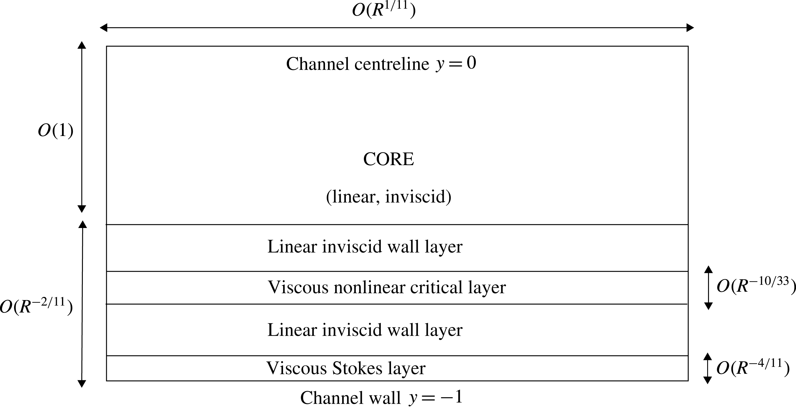
A sketch of the asymptotic structure is given in figure 10. The asymptotic structure within the wall layer is similar to that discussed in § 3 but takes a reduced form due to the long-wavelength effect. The structure outside of the wall layer remains the same as the lower-branch case, but with a smaller wave size.
Motivated by this order of magnitude analysis, we can now derive the asymptotic theory for a viscous nonlinear critical layer structure near the upper neutral branch. We introduce the
 $O(1)$
quantities
 $\unicode[STIX]{x1D6FC}_{0}=R^{1/11}\unicode[STIX]{x1D6FC},X=R^{-1/11}x,c_{0}=R^{2/11}c$
and in the wall layer we express the stream function
 $\unicode[STIX]{x1D713}$
as
 $$\begin{eqnarray}\displaystyle & \displaystyle {\textstyle \frac{1}{2}}\unicode[STIX]{x1D716}^{2}\widehat{\unicode[STIX]{x1D6F9}}_{0}(Y)\text{e}^{\text{i}\unicode[STIX]{x1D6FC}_{0}X}+\text{c.c.}+\text{higher harmonics}, & \displaystyle\end{eqnarray}$$
with
 $y=-1+\unicode[STIX]{x1D6FF}Y$
. Note that
 $\widehat{\unicode[STIX]{x1D6F9}}_{0}$
contains an
 $O(\unicode[STIX]{x1D6FF})$
term that contains the phase jump. The higher-order harmonics in (5.7) are of
 $O(\unicode[STIX]{x1D716}^{2}\unicode[STIX]{x1D6FF})$
, and therefore do not invalidate the assumption of a leading-order monochromatic wave in the core (see (5.14) below). In the wall layer, the leading-order part of the mean flow
 $\overline{u}$
can be calculated solely from the basic PPF as
 $\unicode[STIX]{x1D6FF}Y(2-\unicode[STIX]{x1D6FF}Y)$
. The critical layer location is represented by
 $Y=Y_{c}$
, with
 $Y_{c}$
related to
 $c_{0}$
via
 $$\begin{eqnarray}\displaystyle & \displaystyle c_{0}=2Y_{c}, & \displaystyle\end{eqnarray}$$
and
 $$\begin{eqnarray}\displaystyle & \displaystyle \unicode[STIX]{x1D707}_{c}=y_{c}^{-1}+\cdots =-1+O(\unicode[STIX]{x1D6FF}). & \displaystyle\end{eqnarray}$$
Since the wall layer flow is governed by Rayleigh’s equation we can make use of the general solution (3.12). However, by exploiting the thinness of this region we can simplify the response.
Upon writing
 $z=\unicode[STIX]{x1D6FF}(Y-Y_{c}),a_{0}=a_{00}/\unicode[STIX]{x1D6FF}+a_{01}+\cdots \,,b_{0}=b_{00}+\cdots \,$
in (3.12) and using the small
 $z$
form (3.9) for
 ${\mathcal{P}}_{a}$
and
 ${\mathcal{P}}_{b}$
, the expression (3.5) will yield the desired solution
 $\widehat{\unicode[STIX]{x1D6F9}}_{0}=\widehat{\unicode[STIX]{x1D6F9}}_{0}^{(e)}-\text{i}\widehat{\unicode[STIX]{x1D6F9}}_{0}^{(o)}$
with
 $$\begin{eqnarray}\displaystyle & \displaystyle \widehat{\unicode[STIX]{x1D6F9}}_{0}^{(e)}=a_{00}(Y-Y_{c})+b_{00}, & \displaystyle\end{eqnarray}$$
 $$\begin{eqnarray}\displaystyle & \displaystyle \widehat{\unicode[STIX]{x1D6F9}}_{0}^{(o)}=\unicode[STIX]{x1D6FF}b_{00}(Y-Y_{c})\unicode[STIX]{x1D6E9}, & \displaystyle\end{eqnarray}$$
to leading order. Since the leading-order term in (5.10) must satisfy the impermeability condition on
 $Y=0$
we have
 $$\begin{eqnarray}\displaystyle & \displaystyle b_{00}=a_{00}Y_{c}. & \displaystyle\end{eqnarray}$$
Also, assuming impermeable walls, the boundary pressure is given by
 $$\begin{eqnarray}\displaystyle & \displaystyle \widehat{P}_{0}=c_{0}a_{00}, & \displaystyle\end{eqnarray}$$
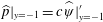
recalling that in this predominantly inviscid region, once the stream function is known we can calculate the pressure; see (3.4) where we can find
 $\widehat{p}|_{y=-1}=c\widehat{\unicode[STIX]{x1D713}}|_{y=-1}^{\prime }$
.
The core flow solution is identical to the lower-branch case except for its size. Since the magnitude of the core stream function is reduced by an
 $O(\unicode[STIX]{x1D6FF})$
amount towards the wall layer and matches to the
 $O(\unicode[STIX]{x1D716}^{2})$
wall layer solution, in the core we have
 $$\begin{eqnarray}\displaystyle & \displaystyle \unicode[STIX]{x1D713}=\unicode[STIX]{x1D716}^{2}\unicode[STIX]{x1D6FF}^{-1}\unicode[STIX]{x1D713}_{0}+\cdots & \displaystyle\end{eqnarray}$$
with
 $\unicode[STIX]{x1D713}_{0}$
given in (4.21). Matching to the wall layer solution (5.10) requires
 $$\begin{eqnarray}\displaystyle & \displaystyle a_{00}=-2\widehat{A}. & \displaystyle\end{eqnarray}$$
Eliminating
 $a_{00}$
and
 $\widehat{P}_{0}$
from (5.13), (5.15) and using the core pressure prediction in (4.22) we find a first relationship between
 $\unicode[STIX]{x1D6FC}_{0}$
and
 $c_{0}$
, namely
 $$\begin{eqnarray}\displaystyle & \displaystyle c_{0}={\textstyle \frac{4}{15}}\unicode[STIX]{x1D6FC}_{0}^{2}. & \displaystyle\end{eqnarray}$$
In order to complete the analysis and find a second relation between these two quantities we need to consider the Stokes layer in more detail. Here the leading-order expansion is
 $$\begin{eqnarray}\displaystyle & \displaystyle \unicode[STIX]{x1D713}=\unicode[STIX]{x1D716}^{2}\unicode[STIX]{x1D6FF}\left\{{\textstyle \frac{1}{2}}\widehat{\unicode[STIX]{x1D711}}({\mathcal{Y}})\text{e}^{\text{i}\unicode[STIX]{x1D6FC}_{0}X}+\text{c.c.}\right\},\quad \widehat{\unicode[STIX]{x1D711}}=\widehat{\unicode[STIX]{x1D711}}^{(e)}-\text{i}\widehat{\unicode[STIX]{x1D711}}^{(o)}, & \displaystyle\end{eqnarray}$$
with the
 $\unicode[STIX]{x1D716}^{2}\unicode[STIX]{x1D6FF}$
factor implied by the arguments leading to (5.4), and
 ${\mathcal{Y}}=(y+1)/\unicode[STIX]{x1D6FF}^{2}$
representing the
 $O(1)$
normal coordinate within the Stokes layer. From substitution into the stream function form of the Navier–Stokes equations (2.7), we find that
 $$\begin{eqnarray}\displaystyle & \displaystyle (\unicode[STIX]{x2202}_{{\mathcal{Y}}}^{2}+\text{i}\unicode[STIX]{x1D6FC}_{0}c_{0})\widehat{\unicode[STIX]{x1D711}}_{{\mathcal{Y}}{\mathcal{Y}}}=0. & \displaystyle\end{eqnarray}$$
It is easy to show that the solution satisfying the no-slip condition on
 ${\mathcal{Y}}=0$
and appropriately matching to the even part of the wall layer solution (5.10) is
 $$\begin{eqnarray}\displaystyle & \displaystyle \widehat{\unicode[STIX]{x1D711}}=a_{00}({\mathcal{Y}}+m^{-1}(\text{e}^{-m{\mathcal{Y}}}-1)),\quad m=m_{0}(1-\text{i}),\quad m_{0}=(\unicode[STIX]{x1D6FC}_{0}c_{0}/2)^{1/2}. & \displaystyle\end{eqnarray}$$
From this solution it is evident that as
 ${\mathcal{Y}}\rightarrow \infty$
the exponential part diminishes and
 $\widehat{\unicode[STIX]{x1D711}}^{(o)}\rightarrow a_{00}/2m_{0}$
. Thus we see explicitly that the Stokes layer solution possesses a non-zero odd contribution. This must match to the odd part of the Rayleigh solution (5.11) as
 $Y\rightarrow 0$
, and thus we conclude
 $$\begin{eqnarray}\displaystyle & \displaystyle -b_{00}Y_{c}\unicode[STIX]{x1D703}=a_{00}/2m_{0}. & \displaystyle\end{eqnarray}$$
Using (5.19) for
 $m_{0}$
, (5.12) for
 $b_{00}$
, and (5.8) for
 $Y_{c}$
, we arrive at
 $$\begin{eqnarray}\displaystyle & \displaystyle -c_{0}^{2}\unicode[STIX]{x1D703}=2^{3/2}(\unicode[STIX]{x1D6FC}_{0}c_{0})^{-1/2}. & \displaystyle\end{eqnarray}$$
For given
 $\unicode[STIX]{x1D703}$
, we can compute
 $\unicode[STIX]{x1D6FC}_{0}$
and
 $c_{0}$
from (5.16) and (5.21); for example substitution of
 $\unicode[STIX]{x1D703}=-\unicode[STIX]{x03C0}$
yields the coefficients
 $(\unicode[STIX]{x1D6FC}_{0},c_{0})=(1.789,0.8536)$
that describe the asymptotic development of the upper branch of the linear neutral curve shown in figure 1. The critical layer analysis given in appendix C describes how to derive an equation that relates
 $\unicode[STIX]{x1D703}$
and a normalised amplitude
 $\unicode[STIX]{x1D6FC}_{0}b_{00}^{3/2}$
.
5.2 Strongly nonlinear critical layer regime
The asymptotic structure of the upper-branch modes at relatively large disturbance amplitudes. Note that the critical layer is now an
 $O(1)$
distance from the channel wall.

Now we consider the modification of this structure that occurs at higher amplitude. In this regime the wavenumber and phase speed of the disturbance are
 $O(1)$
quantities. This shortening of the wavelength leads to a change in the structure within the core region. In particular the perturbed streamwise pressure gradient plays a more active role, with the result that the balances in (4.5) are replaced by a Rayleigh equation for the stream function. This equation is driven by the PPF profile
 $u_{b}$
, since the mean flow distortion is still small. In effect we now have
 $\unicode[STIX]{x1D6FF}\sim O(1)$
, with the inviscid wall layer of the previous section enlarging to fill the entire channel. However, the Stokes layer remains essentially as before; although in view of the
 $O(1)$
size of
 $\unicode[STIX]{x1D6FC}$
and
 $c$
, its thickness
 $d$
is now given, from (5.1), by
 $$\begin{eqnarray}\displaystyle & \displaystyle d=R^{-1/2}. & \displaystyle\end{eqnarray}$$
Once again an odd part of the stream function is induced within this region via the effects of viscosity. Denoting the sizes of the even and odd parts of the stream function by
 $\unicode[STIX]{x1D713}^{(e)},\unicode[STIX]{x1D713}^{(o)}$
we have (since
 $\unicode[STIX]{x1D6FF}\sim O(1)$
):
 $$\begin{eqnarray}\displaystyle & \displaystyle \unicode[STIX]{x1D713}^{(o)}/\unicode[STIX]{x1D713}^{(e)}=O(d); & \displaystyle\end{eqnarray}$$
compare with (5.3). The
 $O(\unicode[STIX]{x1D716})$
thick critical layer is now sited an
 $O(1)$
distance from the wall in view of the largeness of the phase speed. As in § 5.1 there is a balance in this region between the inertial operators
 $u\unicode[STIX]{x2202}_{x}\sim O(\unicode[STIX]{x1D6FC}\unicode[STIX]{x1D716})$
and
 $v\unicode[STIX]{x2202}_{y}\sim O(\unicode[STIX]{x1D6FC}\unicode[STIX]{x1D713}^{(e)}/\unicode[STIX]{x1D716})$
, representing advection by the basic flow and perturbation, respectively. Once again this leads to
 $\unicode[STIX]{x1D713}^{(e)}=O(\unicode[STIX]{x1D716}^{2})$
, but now viscosity is a higher-order effect, with its presence inducing an odd part in the stream function via the inertial-viscous balance
 $\unicode[STIX]{x1D6FC}\unicode[STIX]{x1D713}^{(o)}/\unicode[STIX]{x1D716}\sim R^{-1}\unicode[STIX]{x1D716}^{-2}$
. Hence, since
 $\unicode[STIX]{x1D6FC}\sim O(1)$
, we have
 $$\begin{eqnarray}\displaystyle & \displaystyle \unicode[STIX]{x1D713}^{(o)}/\unicode[STIX]{x1D713}^{(e)}=O(R^{-1}\unicode[STIX]{x1D716}^{-3}). & \displaystyle\end{eqnarray}$$
Reconciling (5.23) and (5.24) we find that the critical layer has increased in thickness to
 $$\begin{eqnarray}\displaystyle & \displaystyle \unicode[STIX]{x1D716}=R^{-1/6}. & \displaystyle\end{eqnarray}$$
A sketch of the new strongly nonlinear stage is given in figure 11.
Guided again by our order-of-magnitude analysis we can now write down the core expansions
 $$\begin{eqnarray}\displaystyle & \displaystyle \unicode[STIX]{x1D713}^{(e)}=\unicode[STIX]{x1D716}^{2}\widehat{\unicode[STIX]{x1D713}}_{0}(y)\cos (\unicode[STIX]{x1D6FC}x)+\cdots \,, & \displaystyle\end{eqnarray}$$
 $$\begin{eqnarray}\displaystyle & \displaystyle \unicode[STIX]{x1D713}^{(o)}=\unicode[STIX]{x1D716}^{5}\{\widehat{\unicode[STIX]{x1D713}}_{1}(y)\sin (\unicode[STIX]{x1D6FC}x)+\text{higher harmonics}\}+\cdots \,, & \displaystyle\end{eqnarray}$$
 $$\begin{eqnarray}\displaystyle & \displaystyle \overline{u}=(1-y^{2})+\unicode[STIX]{x1D716}w(y)+\cdots \,. & \displaystyle\end{eqnarray}$$
Here the leading-order part of
 $\unicode[STIX]{x1D713}^{(e)}$
contains only one Fourier component because a neutral mode solution of the Rayleigh equation can be excited. The presence of a non-trivial mean flow distortion of size
 $O(\unicode[STIX]{x1D716})$
is due to critical layer effects, as we shall see shortly.
The stream function
 $\widehat{\unicode[STIX]{x1D713}}_{0}$
is the Rayleigh solution for
 $\overline{u}=u_{b}$
but now, since the contribution from
 $\unicode[STIX]{x1D713}^{(o)}$
is a higher-order effect, the leading-order phase shift is zero. Thus we can write
 $$\begin{eqnarray}\displaystyle & \displaystyle \widehat{\unicode[STIX]{x1D713}}_{0}=a_{0}\,z\,{\mathcal{P}}_{a}(z)+b_{0}({\mathcal{P}}_{b}(z)+\unicode[STIX]{x1D707}_{c}\,z\,\ln |z|{\mathcal{P}}_{a}(z)), & \displaystyle\end{eqnarray}$$
for both positive and negative
 $z=y-y_{c}$
, where
 ${\mathcal{P}}_{a},{\mathcal{P}}_{b}$
can be computed from (3.8) for given
 $(\unicode[STIX]{x1D6FC},c)$
. Applying the boundary conditions
 $\widehat{\unicode[STIX]{x1D713}}_{0y}=0$
at
 $y=0$
and
 $\widehat{\unicode[STIX]{x1D713}}_{0}=0$
at
 $y=-1$
to (5.29) we obtain an expression of the form
 $$\begin{eqnarray}\displaystyle \left[\begin{array}{@{}cc@{}}H_{0a} & H_{0b}\\ H_{1a} & H_{1b}\end{array}\right]\left[\begin{array}{@{}c@{}}a_{0}\\ b_{0}\end{array}\right]=0, & & \displaystyle\end{eqnarray}$$
where the constants
 $H_{0a},H_{1b},H_{0b},H_{1a}$
can be found by using the values of
 ${\mathcal{P}}_{a}$
and
 ${\mathcal{P}}_{b}$
and their derivatives at
 $y=0,-1$
. Thus we can compute the determinant
 $$\begin{eqnarray}\displaystyle & \displaystyle D=H_{0a}H_{1b}-H_{0b}H_{1a} & \displaystyle\end{eqnarray}$$
as a function of
 $\unicode[STIX]{x1D6FC},c$
and then find the zero locus in order to determine an implicit form of the dispersion relation
 $$\begin{eqnarray}\displaystyle & \displaystyle D(c,\unicode[STIX]{x1D6FC})=0, & \displaystyle\end{eqnarray}$$
as shown by the dashed line in figure 12. Also the value of
 $$\begin{eqnarray}\displaystyle & \displaystyle B(\unicode[STIX]{x1D6FC})\equiv b_{0}^{-1}\widehat{\unicode[STIX]{x1D713}}_{0y}|_{y=-1} & \displaystyle\end{eqnarray}$$
found from the computation along (5.32) is to be used later to fix the undetermined wave amplitude
 $b_{0}$
.
The phase speed
 $c$
and coefficient
 $C$
as functions of wavenumber
 $\unicode[STIX]{x1D6FC}$
in the strongly nonlinear critical layer regime.

As mentioned above, the logarithmic phase shift now occurs at higher order than in the lower-amplitude regime considered previously, and thus
 $\widehat{\unicode[STIX]{x1D713}}_{1}$
can be taken to be zero above the critical layer and non-zero beneath it. The non-zero higher-order flow needs to be reduced in the Stokes layer. The appropriate expansions in the Stokes layer are
 $$\begin{eqnarray}\displaystyle & \displaystyle \unicode[STIX]{x1D713}=\unicode[STIX]{x1D716}^{5}\left\{{\textstyle \frac{1}{2}}\widehat{\unicode[STIX]{x1D711}}({\mathcal{Y}})\text{e}^{\text{i}\unicode[STIX]{x1D6FC}x}+\text{c.c.}\right\}+\cdots \,, & \displaystyle\end{eqnarray}$$
 $$\begin{eqnarray}\displaystyle & \displaystyle \overline{u}=\unicode[STIX]{x1D716}^{3}2{\mathcal{Y}}+\unicode[STIX]{x1D716}^{4}{\mathcal{W}}({\mathcal{Y}})+\cdots \,, & \displaystyle\end{eqnarray}$$
with
 ${\mathcal{Y}}=\unicode[STIX]{x1D716}^{-3}(y+1)$
. The function
 $\widehat{\unicode[STIX]{x1D711}}$
satisfies (5.18) with
 $(\unicode[STIX]{x1D6FC}_{0},c_{0})=(\unicode[STIX]{x1D6FC},c)$
and the appropriate solution is
 $$\begin{eqnarray}\displaystyle \widehat{\unicode[STIX]{x1D711}}=(\widehat{\unicode[STIX]{x1D713}}_{0y}|_{y=-1})\{{\mathcal{Y}}+m^{-1}(\text{e}^{-m{\mathcal{Y}}}-1)\},\quad m=m_{0}(1-\text{i}), & & \displaystyle\end{eqnarray}$$
similar to (5.19) but now
 $m_{0}=(\unicode[STIX]{x1D6FC}c/2)^{1/2}$
. Matching to the core solution we then have
 $$\begin{eqnarray}\displaystyle & \displaystyle \widehat{\unicode[STIX]{x1D713}}_{1}|_{y=-1}=(2m_{0})^{-1}\widehat{\unicode[STIX]{x1D713}}_{0y}|_{y=-1}. & \displaystyle\end{eqnarray}$$
The required phase balance follows from (3.29) as
 $$\begin{eqnarray}\displaystyle b_{0}[\widehat{\unicode[STIX]{x1D713}}_{1y}]_{y=y_{c-}}^{y_{c+}}=\frac{(\widehat{\unicode[STIX]{x1D713}}_{0y}|_{y=-1})^{2}}{2m_{0}}, & & \displaystyle\end{eqnarray}$$
which is analogous to the weakly nonlinear result (5.20).
The critical layer analysis proceeds much along the lines of that presented in § 3, and the details are given in appendix D, where it is shown that the total stream function
 $\unicode[STIX]{x1D713}+\int \overline{u}\,\text{d}y$
possesses an asymptotic expansion
 $\unicode[STIX]{x1D6F7}=\unicode[STIX]{x1D716}^{2}\unicode[STIX]{x1D6F7}_{1}(x,Z)+\cdots \,$
, with
 $\unicode[STIX]{x1D6F7}_{1}$
given in (3.20), and where
 $Z=\unicode[STIX]{x1D716}^{-1}(y-y_{c})$
is the
 $O(1)$
normal variable in the critical layer with the thickness (5.25). The corresponding total vorticity is
 $$\begin{eqnarray}\displaystyle & \displaystyle \unicode[STIX]{x1D714}=2y_{c}-\unicode[STIX]{x1D716}K(\unicode[STIX]{x1D701})+\cdots \,;\quad \unicode[STIX]{x1D701}=\unicode[STIX]{x1D6F7}_{1}/b_{0} & \displaystyle\end{eqnarray}$$
with the function
 $K$
governed by inviscid dynamics. The streamlines of constant
 $\unicode[STIX]{x1D701}$
form a familiar Kelvin’s cats-eye pattern with the separatrices
 $$\begin{eqnarray}\displaystyle & \displaystyle Z=Z_{\pm }(x)\equiv w_{c}/2y_{c}\pm (-b_{0}/y_{c})^{1/2}[1-\cos (\unicode[STIX]{x1D6FC}x)]^{1/2}, & \displaystyle\end{eqnarray}$$
obtained by setting
 $\unicode[STIX]{x1D701}=1$
, defining the edge of the eye. Within the eye all the streamlines are closed. A plot of the streamlines is given in figure 13.


In order to determine the precise form of
 $K$
we need to proceed to higher order to include viscous effects. The analysis in appendix D shows that
 $$\begin{eqnarray}\displaystyle K(\unicode[STIX]{x1D701})=\left\{\begin{array}{@{}ll@{}}\displaystyle K_{0}\pm 2^{1/2}\unicode[STIX]{x03C0}C\int _{1}^{\unicode[STIX]{x1D701}}\frac{1}{I(\unicode[STIX]{x1D701}_{\ast })}\,\text{d}\unicode[STIX]{x1D701}_{\ast }, & \unicode[STIX]{x1D701}>1,\\ K_{0} & \unicode[STIX]{x1D701}<1,\end{array}\right. & & \displaystyle\end{eqnarray}$$
where
 $$\begin{eqnarray}\displaystyle & \displaystyle I(\unicode[STIX]{x1D701})=\int _{0}^{2\unicode[STIX]{x03C0}}(\unicode[STIX]{x1D701}-\cos \unicode[STIX]{x1D709})^{1/2}\,\text{d}\unicode[STIX]{x1D709} & \displaystyle\end{eqnarray}$$
and the
 $\pm$
sign corresponds to the upper/lower regions wherein
 $Z>Z_{+}\text{ and }Z<Z_{-}$
. The fact that inside of the cats eye
 $K$
is a constant is a consequence of the Prandtl–Batchelor theorem (Batchelor Reference Batchelor1956). The explicit form of the coefficient
 $C(b_{0})$
can be found by matching to be
 $$\begin{eqnarray}\displaystyle & \displaystyle C=-(-2b_{0}/y_{c})^{1/2}, & \displaystyle\end{eqnarray}$$
which follows from the analysis in appendix D leading to (D 7).
With the function
 $K$
determined, we can now calculate the jumps in velocity and mean shear across the critical layer. These are shown in appendix D to take the form
 $$\begin{eqnarray}\displaystyle & \displaystyle [\widehat{\unicode[STIX]{x1D713}}_{1y}]_{y=y_{c-}}^{y_{c+}}=-\frac{4C\unicode[STIX]{x1D6EC}}{\unicode[STIX]{x1D6FC}b_{0}}, & \displaystyle\end{eqnarray}$$
 $$\begin{eqnarray}\displaystyle & \displaystyle w_{y}|_{y=y_{c+}}=-C\unicode[STIX]{x1D6EC}+K_{0},\quad w_{y}|_{y=y_{c-}}=C\unicode[STIX]{x1D6EC}+K_{0}, & \displaystyle\end{eqnarray}$$
where the constant
 $\unicode[STIX]{x1D6EC}\approx 1.379$
. Substituting (3.26), (5.33), (5.43) and (5.44) into (5.38), we can write down an explicit formula for the amplitude
 $b_{0}$
:
 $$\begin{eqnarray}\displaystyle & \displaystyle b_{0}=\left(\frac{c}{\unicode[STIX]{x1D6FC}\sqrt{1-c}}\right)^{1/3}\left(\frac{8\unicode[STIX]{x1D6EC}}{B^{2}}\right)^{2/3}. & \displaystyle\end{eqnarray}$$
Once the value of
 $B$
is obtained from the Rayleigh solution, the amplitude obtained above can be used to calculate
 $C$
through (5.43) as a function of
 $\unicode[STIX]{x1D6FC}$
, as shown in figure 12. As we shall see shortly, the mean flow distortion has vanishing shear for
 $y\in (y_{c},0]$
. Therefore, from (5.45), we can fix the value of the uniform vorticity as
 $K_{0}=C\unicode[STIX]{x1D6EC}$
.
5.3 Comparison of nonlinear upper-branch Navier–Stokes and asymptotic computations
The bifurcation diagram on the viscous nonlinear critical layer scale. The black solid curves are Navier–Stokes results for
 $R=10^{6},10^{7},10^{8},10^{9}$
. The filled circle at (a) is the same point that appears in figure 2. The red dashed curve is the asymptotic result (5.16), (5.21). The magenta crosses are the bifurcation points.

After the bifurcation from the upper branch of the neutral curve, the travelling wave first develops a viscous nonlinear critical layer and thus the asymptotic theory of § 5.1 is relevant here. Figure 14 shows the bifurcation diagram scaled appropriately to this asymptotic regime. It is known that the convergence towards this limit is rather slow (see, for example, figure 1), and thus here we plot the Navier–Stokes results up to
 $R=10^{9}$
as the black solid curves. The red dashed curve is calculated using the asymptotic result (5.16) and (5.21), varying the phase shift
 $\unicode[STIX]{x1D703}$
from
 $-\unicode[STIX]{x03C0}$
to zero. As mentioned earlier, the linear critical point
 $(\unicode[STIX]{x1D6FC}_{0},c_{0})=(1.789,0.8536)$
corresponds to the case
 $\unicode[STIX]{x1D703}=-\unicode[STIX]{x03C0}$
. As the amplitude of the wave instability is increased, the modulus of phase
 $|\unicode[STIX]{x1D703}|$
is reduced and the values of
 $\unicode[STIX]{x1D6FC}_{0}=R^{1/11}\unicode[STIX]{x1D6FC}$
and
 $c_{0}=R^{2/11}c$
will increase. Eventually the wavenumber and phase speed of the travelling wave states become
 $O(1)$
, and thus we enter the strongly nonlinear critical layer regime where the majority of the flow is governed by the Rayleigh equation.
The bifurcation diagram on the strongly nonlinear critical layer scale. The black solid curves are Navier–Stokes results for
 $R=10^{5},10^{6},10^{7}$
. The filled circle at (b) is the same point that appears in figure 2. The red dashed curve is the result from figure 12, obtained by solving the Rayleigh equation with zero phase shift. The magenta crosses are the bifurcation points.

The flow near the critical level
 $y=y_{c}$
for
 $c=0.27$
. In the figures we subtract the basic shear contribution
 $2y_{c}$
from the total vorticity, and rescale by dividing by
 $\unicode[STIX]{x1D716}=R^{-1/6}$
. Colour shows
 $\unicode[STIX]{x1D716}^{-1}(\unicode[STIX]{x1D714}-2y_{c})$
, and its range is
 $[C_{min},C_{max}]=[-1,3.6]$
. The vertical coordinate is
 $Z=\unicode[STIX]{x1D716}^{-1}(y-y_{c})$
. (a) shows the Navier–Stokes results at point (b) in figure 2 with
 $R=10^{6}$
. (b) is the theoretical result
 $-K$
, where
 $K(\unicode[STIX]{x1D701})$
is given in (5.41).

The scaled mean flow distortion
 $\unicode[STIX]{x1D716}^{-1}(\overline{u}-u_{b})$
for
 $c=0.27$
, with
 $\unicode[STIX]{x1D716}=R^{-1/6}$
. The black solid curves are Navier–Stokes results for
 $R=10^{5},10^{6},10^{7}$
. The dashed curve is the asymptotic result (5.47).

The Navier–Stokes solution curves plotted in figure 15 show excellent agreement with the dispersion relation (5.32) arising from the solution of Rayleigh’s equation (taken from figure 12), and shown here by the red dashed curve. At the point (b) the phase speed is close to
 $c=0.27$
. The flow in the critical layer is expected to develop a Kelvin’s cats-eye pattern, so in the subsequent figures we provide a detailed visual comparison of the Navier–Stokes and asymptotic results at this value of
 $c$
. The vorticity in the neighbourhood of the critical level is compared in figure 16. In these plots we subtract the contribution of vorticity due to the basic flow,
 $2y_{c}$
, in view of (5.39), and then divide by
 $\unicode[STIX]{x1D716}$
. The asymptotic and Navier–Stokes results are in good agreement and a cats-eye pattern is indeed observed.
We can also compare the flux of the Navier–Stokes and asymptotic solutions. For the strongly nonlinear critical layer case, the mean flow in the core expands as
 $\overline{u}=u_{b}(y)+R^{-1/6}w(y)+\cdots \,$
. In view of the lack of forcing there, see remark (ii) in § 3, the mean flow distortion in the core must assume a piecewise linear form
 $$\begin{eqnarray}\displaystyle w(y)=\left\{\begin{array}{@{}ll@{}}M(y_{c}+1) & \text{if}\,y\in (y_{c},0],\\ M(y+1) & \text{if}\,y\in [-1,y_{c}),\end{array}\right. & & \displaystyle\end{eqnarray}$$
with the constant
 $M$
determined from the jump condition (5.45) as
 $$\begin{eqnarray}\displaystyle & \displaystyle M=2C\unicode[STIX]{x1D6EC}. & \displaystyle\end{eqnarray}$$
Here it should be noted that the shear stress associated with the mean flow distortion must vanish on the wall, because the imposed constant pressure gradient is in balance with the basic shear on the wall. In fact, if the Reynolds stress in (2.6c ) is calculated using (5.36), then the mean flow distortion in the Stokes layer can be determined explicitly as
 $$\begin{eqnarray}\displaystyle \displaystyle {\mathcal{W}}({\mathcal{Y}}) & = & \displaystyle M{\mathcal{Y}}-\frac{b_{0}^{2}B^{2}}{4c}\left\{2(m_{0}{\mathcal{Y}}+2)\text{e}^{-m_{0}{\mathcal{Y}}}\cos (m_{0}{\mathcal{Y}})\right.\nonumber\\ \displaystyle & & \displaystyle \left.+\,2(m_{0}{\mathcal{Y}}-1)\text{e}^{-m_{0}{\mathcal{Y}}}\sin (m_{0}{\mathcal{Y}})-\text{e}^{-2m_{0}{\mathcal{Y}}}-3\right\},\end{eqnarray}$$
upon application of the no-slip condition on
 ${\mathcal{Y}}=0$
and the matching to (5.47) as
 ${\mathcal{Y}}\rightarrow \infty$
. Using this expression we can confirm analytically that
 ${\mathcal{W}}_{{\mathcal{Y}}}=0$
at
 ${\mathcal{Y}}=0$
, which provides an important check on the asymptotic analysis. The convergence of the Navier–Stokes solution with increasing Reynolds number to the asymptotic state can be seen in the comparison of the corresponding mean flow distortions, shown in figure 17 with the asymptotic solution represented by a dashed line. We can establish a similar mean flow distortion for the viscous nonlinear critical layer regime, as shown in appendix C. These asymptotic forms for the distortion can be used to establish how the leading-order flux scales with Reynolds number. We find
 $$\begin{eqnarray}\displaystyle & \displaystyle 1-Q\approx -R^{-16/33}\frac{3M_{0}c_{0}}{4}, & \displaystyle\end{eqnarray}$$
with
 $M_{0}$
given in (C 10) for the viscous nonlinear critical layer regime, and
 $$\begin{eqnarray}\displaystyle & \displaystyle 1-Q\approx -R^{-1/6}\frac{3Mc}{4}, & \displaystyle\end{eqnarray}$$
with
 $M$
given in (5.48) for the strongly nonlinear critical layer regime. The comparison with the Navier–Stokes results again shows a good agreement, as can be seen in figure 18.
6 Conclusion and discussions

In this paper we have clarified how nonlinear travelling wave solutions in plane Poiseuille flow bifurcate from the linear neutral curve at large Reynolds numbers, and how they develop as the amplitude of the wave is increased. We have computed Navier–Stokes solutions at higher resolution and Reynolds number than previous authors and, on the basis of the results we have obtained, it can now be stated conclusively that the behaviour of the solutions is accurately captured by the known asymptotic theories, at least in the relatively-small- to moderate-amplitude regime. On the other hand, the asymptotic behaviours of large-amplitude states are unexplained on the basis of existing theories. Our key findings are summarised below. Here (a)–(f) correspond to the points appearing in figures 2 and 3.
(a) Near the upper neutral curve, the asymptotic behaviour of the travelling waves can be explained by viscous nonlinear critical layer theory. The effects of nonlinearity are confined to the critical layer, while in the remainder of the channel the disturbance is of monochromatic wave form to leading order. That overall asymptotic structure derived in § 5.1 is identical to that developed by Smith & Bodonyi (Reference Smith and Bodonyi1982a
) for boundary layer flows, except for the different form of pressure–displacement law in the core region that also causes the minor change in the asymptotic scaling. For channel flow, the wave has a long streamwise scale of
 $O(R^{1/11})$
, and induces a mean flow distortion of
 $O(R^{-16/33})$
. The critical layer sits in a near-wall zone and thus the solution smoothly connects to the neutral curve; see the remark in § 3.2. With increasing wave amplitude, the asymptotic structure breaks down as the critical layer eventually becomes detached from the wall region.


(b) A strongly nonlinear critical layer emerges at the next disturbance level and is now completely detached from the wall. Here the flow is predominantly inviscid, so that it is characterised by a constant vorticity region of cat’s eye shape. Again, to leading order, the nonlinear effects only appear in the critical layer, with the mean flow distortion suffering a stress jump across it. The typical streamwise scale becomes
 $O(1)$
, and the mean flow distortion is of
 $O(R^{-1/6})$
. The asymptotic theory derived in § 5.2 was obtained by modifying the theory developed by Bodonyi et al. (Reference Bodonyi, Smith and Gajjar1983) for boundary layer flows. Furthermore, in our paper an explicit asymptotic form for the mean flow distortion is derived and confirmed to give an excellent prediction of the Navier–Stokes results. As suggested in figure 12, at large amplitude the phase speed tends to unity. The breakdown of the asymptotic structure occurs when the critical layer approaches the centre of the channel, where the basic shear becomes small.
(c) The constant vorticity region thickens in the vertical direction, and the streamwise scale becomes shorter. Smith, Doorly & Rothmayer (Reference Smith, Doorly and Rothmayer1990) considered the large-amplitude limit of the strongly nonlinear critical layer theory and derived a ‘nonlinear slug layer’ theory. The theory may be of relevance to this regime, and is briefly summarised in appendix E, together with some more detailed analysis within the slug layer. The key point of the theory is that now the nonlinear interaction is concentrated in the slug layer around the centre of the channel and the flow is governed by the Euler equations. Since the dynamics there is predominantly inviscid, the flow is approximately symmetric in
 $x$
, and a constant vorticity zone is present if the streamlines are closed. The slug layer thickness is much thicker than the critical layers in regimes (a) and (b), being of
 $O(1/\ln R)$
. All these observations are consistent with figure 3(c). Moreover, for point (c) we have
 $1-c=0.78$
and, from (E 14), the mean flow distortion for negative
 $y$
is approximately
 $1-y^{2}-(1-c)(1+y)$
, which predicts the centreline velocity to be
 $1-0.78=0.22$
. The thickness of the slug region is comparable to the streamwise scale and can be estimated as
 $1/\unicode[STIX]{x1D6FC}=1/1.95=0.51$
. All in all, these values are not far away from those associated with the profile at point (c) given in figure 4, so the size of the mean flow correction predicted by the theory is, roughly speaking, in agreement with the numerical results. In this regard figure 19 is also encouraging as it seems to show that the scaling of the slug layer stage is appropriate, although the asymptotic convergence is not perfect at this level of
 $R$
, probably because the typical perturbation parameter of the theory is
 $O(1/\ln R)$
, which of course is not particularly small at the Reynolds numbers we have computed. Also, unfortunately, the computation of the slug layer asymptotic problem is extremely difficult and not attempted here. Note that the asymptotic slug problem is fundamentally different from recently found three-dimensional states localised around the channel centre, where the structure is fully viscous, and hence the asymptotic convergence is better (Deguchi Reference Deguchi2015).
(d) The computed flow field is now characterised by the thin layered structure near the wall that seems to eventually detach from the boundary along the edge of the vortex bubble. The asymptotic regime corresponding to this point is unknown and discussed further in (f) below. We could not complete the loop connecting the upper and lower neutral curves due to the numerical difficulty at large
 $R$
, but according to bifurcation theory, the topology of the solution branch should not alter when
 $R$
is changed (unless the branches collide with a hitherto undiscovered solution branch, and provided one believes that the Navier–Stokes equations are free of singularities), and thus the branches continued from the upper and lower neutral curves are expected to eventually meet. Therefore, it is likely that this regime connects to the point (f), where the flow is also characterised by a similar flow structure.
(e) Near the lower neutral curve, we can formulate a nonlinear double-deck theory. Although similar nonlinear triple-deck equations were studied for example in Hall (Reference Hall1995) for boundary layer flows, the nonlinear double-deck theory valid for channel flows is derived and solved in § 4.1 for the first time. The typical streamwise scale is
 $O(R^{2/7})$
, and the mean flow distortion is
 $O(R^{-2/7})$
. The critical layer is in the near-wall region, and thus the solution connects smoothly to the linear neutral point. The computational results arising from both the solutions of the asymptotic problem and the Navier–Stokes equations indicate that with increasing wave amplitude there is a development of a short streamwise scale that may lead to the breakdown of the asymptotic theory. After the breakdown, the regime (f) will appear and thus, although the form of the breakdown appears to be somewhat different, the present result supports the observation by Hall (Reference Hall1995), who noticed that the analogous lower-branch state for boundary layer flow is unlikely to have a direct connection to the Euler slug stage explained in (c).
(f) The computed flow field is similar to that observed at (d), except that the vortex bubble sits in the near-wall zone; inside of the vortex bubble the vorticity is constant, so the dynamics there would be inviscid as the Prandtl–Batchelor theorem suggests. The separated thin near-wall structure straddles the edge of the constant vorticity zone, creating a vorticity jump there. That ‘separation’ seems to be a signature of a strong interaction between the thin near-wall structure and the vortex bubble, and so the nonlinearity may no longer be concentrated in a thin horizontal layer as is the case with the known theories. The broken quasi symmetry in
 $x$
there implies that the separation process is viscous. The mathematical description of this asymptotic regime is unknown, but the Navier–Stokes results here may be used for guidance in possibly deriving it in the future.
The above observations imply that laminar-turbulent transition of a high-speed channel flow is an extremely rich process even when it is restricted to two-dimensional space. When a small spanwise independent perturbation is introduced in the flow, it will experience various asymptotic states before reaching a turbulent state. As the linear theory predicts, infinitesimally small growing perturbations must possess long wavelengths with strong vorticity occurring near the wall. However, as the circulation within the critical layer becomes stronger, its aspect ratio approaches unity, so that the natural disturbance wavelength is shortened and the width of the critical layer is thickened. This seems to be consistent with a previous study by Jimenez (Reference Jimenez1990), who performed direct numerical simulations of two-dimensional channel flow at Reynolds numbers of order
 $10^{4}$
. Various streamwise length scales were observed even in the final turbulent states when a sufficiently long periodic box was chosen. The chaotic wave packets shown in figures 10 and 12 of that paper are locally reminiscent of the result shown in our figure 3. Those figures suggest that seemingly there are two streamwise scales in the simulation: the first one is associated with the oscillation of the wave-like structure, while the other describes the slower development of the wave amplitude. This means that a connection between our results and the simulations could be found using a Wentzel–Kramers–Brillouin (WKB) approach, thereby offering a physical explanation why the local wavelength of the wave packets shortens as the local amplitude increases.
Moreover, it is noteworthy that the existence of localised time periodic solutions has been reported by Price, Brachet & Pomeau (Reference Price, Brachet and Pomeau1993) at lower Reynolds numbers, and recently Mellibovsky & Meseguer (Reference Mellibovsky and Meseguer2015) found similar solutions from a bifurcation analysis of the usual TS wave solution branch. A dynamical systems theory approach is often used to relate time-periodic solutions and flow dynamics. Thus if one believes that the time-periodic solutions form a backbone of chaotic wave packets observed in the simulations, they could be used to prove the above conjecture. Interestingly, the wave packet seen in the time-periodic solution is fully localised in the streamwise direction – namely when the local amplitude of the wave becomes small, the local wavelength increases so that the flow heads back towards its undisturbed state. It is noteworthy that the longest possible wavelength of the nonlinear wave is of
 $O(R)$
, as Deguchi & Walton (Reference Deguchi and Walton2013a
) showed. This flow regime is a two-dimensional counterpart of Deguchi et al. (Reference Deguchi, Hall and Walton2013), and is therefore governed by Prandtl’s boundary layer equations, but with an
 $O(1)$
vertical scale and driven by an unknown pressure gradient that is determined as part of the solution. As is the case for the three-dimensional study, the two-dimensional long-wavelength scale structure holds across the entire channel.
Among the asymptotic structures listed at the beginning of this section, of course the unknown asymptotic states (d,f) appearing at the highest amplitude are the most interesting. The numerical simulations show that when the local amplitude of the wave packet takes its maximum value the flow is characterised by a sweeping of the near-wall region that results in the ejection of plume-like structures from the boundary layer into the fluid core. This is precisely what is seen in the state (d) of the present study. The numerical observations and asymptotic analysis in this paper reveal that this regime is encountered when the thickness of the critical layer becomes comparable to the channel width, and the vortices within the layer directly interact with the wall boundary layer. At this stage the mean flow distortion becomes as large as the basic flow (see figure 4), so there seems to be a feedback effect from the mean flow distortion to the instability wave, and the analysis may become more complicated. This possible self-sustainment mechanism is remarkable, because all known two-dimensional asymptotic theories assume a small mean flow distortion and therefore, in this sense, all small-amplitude travelling waves are solely triggered by some instability of the basic flow. Although the structure of the vortices in the core region can be fully understood by appealing to the Prandtl–Batchelor theorem, the mathematical description of the sweep and ejection process is as yet unknown. That description is exactly what hinders the formulation of a closure that could possibly be used to predict the turbulent mean profile associated with high-speed two-dimensional flows.
Furthermore, we note that the formation of the Prandtl–Batchelor zone and the boundary layer seems to be ubiquitous even for three-dimensional flows. For example, Deguchi & Hall (Reference Deguchi and Hall2014b ) found that three-dimensional solutions of plane Couette flow develop a constant streamwise vorticity region at large amplitude. Vortex–wave interaction theory, which is often used to elucidate the sustainment mechanism of three-dimensional solutions, failed to explain the appearance of that Prandtl–Batchelor zone and the boundary layer because the theory assumes fully viscous streamwise vortices. The unknown interaction process between those two regions is again the key to completing the corresponding asymptotic closure. We hope an investigation of the simpler two-dimensional state found here will also provide some clue as to how this more complicated problem may be solved in the future.
Acknowledgements
This work was partially supported by Australian Research Council Australian Discovery Early Career Award DE170100171.
Appendix A. Basis functions in the numerical analysis
A.1 Full Navier–Stokes computation
In order to use a Chebyshev expansion in the computation, the vertical variable
 $y\in [-1,0]$
is mapped to
 $$\begin{eqnarray}\displaystyle & \displaystyle \unicode[STIX]{x1D702}=\frac{\widetilde{y}-y}{y+2y\widetilde{y}+\widetilde{y}}\in [-1,1], & \displaystyle\end{eqnarray}$$
using a map parameter
 $\widetilde{y}$
. Note that the intervals
 $[-1,\widetilde{y})$
and
 $(\,\widetilde{y},0]$
have the same number of collocation points. The basis functions in expansion (2.12) are defined as
 $$\begin{eqnarray}\displaystyle & \displaystyle f_{l}^{(0)}(\unicode[STIX]{x1D702})=(1-\unicode[STIX]{x1D702})(1+\unicode[STIX]{x1D702})^{2}[(1-\unicode[STIX]{x1D702})T_{l}(\unicode[STIX]{x1D702})+c_{l}^{(0)}], & \displaystyle\end{eqnarray}$$
 $$\begin{eqnarray}\displaystyle & \displaystyle f_{l}^{(1)}(\unicode[STIX]{x1D702})=(1+\unicode[STIX]{x1D702})^{2}[(1-\unicode[STIX]{x1D702})^{2}T_{l}(\unicode[STIX]{x1D702})+c_{l}^{(1)}(\unicode[STIX]{x1D702}^{2}-3)], & \displaystyle\end{eqnarray}$$
 $$\begin{eqnarray}\displaystyle & \displaystyle g_{l}(\unicode[STIX]{x1D702})=(1+\unicode[STIX]{x1D702})[(1-\unicode[STIX]{x1D702})T_{l}(\unicode[STIX]{x1D702})+2], & \displaystyle\end{eqnarray}$$
using
 $l$
th-order Chebyshev polynomials
 $T_{l}$
. It is easy to confirm that
 $f_{l}^{(0)}=f_{ly}^{(0)}=f_{l}^{(1)}=f_{ly}^{(1)}=g_{l}=0$
at
 $y=-1$
,
 $f_{l}^{(0)}=f_{ly}^{(1)}=g_{ly}=0$
at
 $y=0$
. In order to satisfy
 $f_{lyy}^{(0)}=f_{lyyy}^{(1)}=0$
at
 $y=0$
we must use the coefficients
 $$\begin{eqnarray}\displaystyle & \displaystyle c_{l}^{(0)}=2\frac{\widetilde{y}+1}{4\widetilde{y}+3},\quad c_{l}^{(1)}=-2\frac{l^{2}(\widetilde{y}+1)+(3\widetilde{y}+2)}{13\widetilde{y}+8}. & \displaystyle\end{eqnarray}$$
A.2 Lower-branch computation
Likewise for the lower-branch computation we use the mapping
 $$\begin{eqnarray}\displaystyle & \displaystyle \unicode[STIX]{x1D702}=\frac{\widetilde{y}-(Y/H-1)}{(Y/H-1)+2(Y/H-1)\widetilde{y}+\widetilde{y}}\in [-1,1], & \displaystyle\end{eqnarray}$$
to map
 $Y\in [0,H]$
, where
 $H$
, the upper bound of the computational domain, is taken to be sufficiently large. The basis functions in expansion (4.15) are chosen to satisfy
 $G_{l}=F_{l}^{(0)}=F_{lY}^{(0)}=F_{l}^{(1)}=F_{lY}^{(1)}=0$
at
 $Y=0$
,
 $G_{lY}=2$
and
 $F_{lY}^{(0)}=F_{lYY}^{(1)}=0$
at
 $Y=H$
, and take the form:
 $$\begin{eqnarray}\displaystyle F_{l}^{(j)}(\unicode[STIX]{x1D702})=(1+\unicode[STIX]{x1D702})^{2}[(1-\unicode[STIX]{x1D702})T_{l}(\unicode[STIX]{x1D702})+c_{l}^{(j)}],\quad G_{l}(\unicode[STIX]{x1D702})=(1+\unicode[STIX]{x1D702})[(1-\unicode[STIX]{x1D702})T_{l}(\unicode[STIX]{x1D702})+2], & & \displaystyle\end{eqnarray}$$
where
 $$\begin{eqnarray}\displaystyle c_{l}^{(0)}=1,\quad c_{l}^{(1)}=4\frac{(1+\widetilde{y})(1+l^{2})+\widetilde{y}}{(1+5\widetilde{y})}. & & \displaystyle\end{eqnarray}$$
Appendix B. The phase jump in the viscous nonlinear critical layer equation
Dropping the tildes for the sake of simplicity, the key equation (3.22) in the viscous nonlinear critical layer can be written in the following form:
 $$\begin{eqnarray}\displaystyle & \displaystyle (Z\unicode[STIX]{x2202}_{\unicode[STIX]{x1D709}}+\sin \unicode[STIX]{x1D709}\unicode[STIX]{x2202}_{Z})F=\unicode[STIX]{x1D6FE}F_{ZZ}, & \displaystyle\end{eqnarray}$$
 $$\begin{eqnarray}\displaystyle & \displaystyle F(\unicode[STIX]{x1D709},Z)\rightarrow Z+\frac{\unicode[STIX]{x1D703}}{4\unicode[STIX]{x1D6FE}}\text{sgn}(Z)+\text{const.}+Z^{-1}\cos \unicode[STIX]{x1D709}+\cdots \quad \text{as}\,|Z|\rightarrow \infty , & \displaystyle\end{eqnarray}$$
where
 $\unicode[STIX]{x1D6F7}_{ZZ}=F(\unicode[STIX]{x1D709},Z)$
satisfies the periodic and symmetric conditions
 $$\begin{eqnarray}\displaystyle F(\unicode[STIX]{x1D709},Z)=F(\unicode[STIX]{x1D709}+2\unicode[STIX]{x03C0},Z),\quad F(\unicode[STIX]{x1D709},Z)=-F(-\unicode[STIX]{x1D709},-Z), & & \displaystyle\end{eqnarray}$$
respectively. In order to find the phase jump
 $\unicode[STIX]{x1D703}$
, we need to solve the above system numerically. Expanding
 $F$
in a Fourier series, equation (B 1) is converted into a set of equations for the Fourier coefficients that can be marched in
 $Z$
using the Runge–Kutta method. Due to the symmetry involved we only need to integrate this equation for positive
 $Z$
. The initial conditions at
 $Z=0$
need to be controlled so that the mean part of
 $F_{Z}$
tends to 1 and to ensure there is no exponential growth for large
 $Z$
. The result we obtain, shown in figure 20, is entirely consistent with those of Haberman (Reference Haberman1972) and Smith & Bodonyi (Reference Smith and Bodonyi1982a
), who demonstrated that further integration of
 $F$
with respect to
 $Z$
produces the required logarithmic term and the jump term
 $J(\unicode[STIX]{x1D709})$
which appears in (3.23) for large
 $|Z|$
; note that
 $J(\unicode[STIX]{x1D709})$
must be an odd function due to the symmetry (B 3). The latter authors also derived the asymptotic result
 $\unicode[STIX]{x1D703}\rightarrow -4\unicode[STIX]{x1D6EC}\unicode[STIX]{x1D6FE}$
, (with
 $\unicode[STIX]{x1D6EC}$
the constant obtained in (D 6)) as
 $\unicode[STIX]{x1D6FE}\rightarrow 0$
, and this is also shown on figure 20. The other limiting behaviour
 $\unicode[STIX]{x1D703}\rightarrow -\unicode[STIX]{x03C0}$
as the amplitude
 $\unicode[STIX]{x1D6FE}^{-1}\rightarrow 0$
is the classical linear phase shift result and can be easily shown, as demonstrated below.
The phase shift
 $\unicode[STIX]{x1D703}$
for various
 $\unicode[STIX]{x1D6FE}$
. The red dashed lines are the small-
 $\unicode[STIX]{x1D6FE}$
asymptotic result
 $\unicode[STIX]{x1D703}=-4\unicode[STIX]{x1D6EC}\unicode[STIX]{x1D6FE}$
and the large-
 $\unicode[STIX]{x1D6FE}$
asymptotic result
 $\unicode[STIX]{x1D703}=-\unicode[STIX]{x03C0}$
.

First we write
 $F$
in the normal mode form
 $$\begin{eqnarray}\displaystyle & \displaystyle F=\{Z+\unicode[STIX]{x1D6FE}^{-1}\overline{f}(\unicode[STIX]{x1D702})+\cdots \,\}+\{\unicode[STIX]{x1D6FE}^{-1/3}\widetilde{f}(\unicode[STIX]{x1D702})+\cdots \,\}\text{e}^{\text{i}\unicode[STIX]{x1D709}}+\text{c.c.} & \displaystyle\end{eqnarray}$$
with
 $\unicode[STIX]{x1D702}=\unicode[STIX]{x1D6FE}^{-1/3}Z$
. Clearly we require
 $\overline{f}(\unicode[STIX]{x1D702})\rightarrow \pm \unicode[STIX]{x1D703}/4$
as
 $\unicode[STIX]{x1D702}\rightarrow \pm \infty$
, in view of the matching conditions (B 2). Substituting (B 4) to (B 1), at leading order we obtain
 $$\begin{eqnarray}\displaystyle & \displaystyle (\text{i}\unicode[STIX]{x1D702}-\unicode[STIX]{x2202}_{\unicode[STIX]{x1D702}}^{2})\widetilde{f}=\text{i}/2, & \displaystyle\end{eqnarray}$$
 $$\begin{eqnarray}\displaystyle & \displaystyle \frac{1}{2}\int _{-\infty }^{\infty }\{\text{i}\widetilde{f}+\text{c.c.}\}\text{d}\unicode[STIX]{x1D702}=\left[\,\overline{f}\,\right]_{-\infty }^{\infty }=\frac{\unicode[STIX]{x1D703}}{2}. & \displaystyle\end{eqnarray}$$
The bounded solution of (B 5) is
 $$\begin{eqnarray}\displaystyle & \displaystyle \widetilde{f}(\unicode[STIX]{x1D702})={\displaystyle \frac{\text{i}}{2}}\int _{0}^{\infty }\text{e}^{-\text{i}t\unicode[STIX]{x1D702}-t^{3}/3}\text{d}t. & \displaystyle\end{eqnarray}$$
It follows that
 $$\begin{eqnarray}\displaystyle \displaystyle \int ^{\unicode[STIX]{x1D702}}\widetilde{f}(\unicode[STIX]{x1D702}_{\ast })\text{d}\unicode[STIX]{x1D702}_{\ast } & = & \displaystyle \frac{1}{2}\int _{0}^{\infty }\text{e}^{-t^{3}/3}(1-\text{e}^{-\text{i}t\unicode[STIX]{x1D702}})/t\,\text{d}t+\text{const.}\nonumber\\ \displaystyle & = & \displaystyle {\displaystyle \frac{\text{i}}{2}}\int _{0}^{\infty }\frac{\sin (t\unicode[STIX]{x1D702})}{t}\text{d}t+r(\unicode[STIX]{x1D702})+\text{real function}+\text{const.}\nonumber\\ \displaystyle & = & \displaystyle \text{i}{\displaystyle \frac{\unicode[STIX]{x03C0}}{4}}\text{sgn}(\unicode[STIX]{x1D702})+r(\unicode[STIX]{x1D702})+\text{real function}+\text{const.},\end{eqnarray}$$
where
 $$\begin{eqnarray}\displaystyle & \displaystyle r(\unicode[STIX]{x1D702})={\displaystyle \frac{1}{2}}\int _{0}^{\infty }{\displaystyle \frac{1-\text{e}^{-t^{3}/3}}{t}}\text{e}^{-\text{i}t\unicode[STIX]{x1D702}}\,\text{d}t. & \displaystyle\end{eqnarray}$$
We can then establish by integration by parts that
 $r(\unicode[STIX]{x1D702})\rightarrow 0$
as
 $|\unicode[STIX]{x1D702}|\rightarrow \infty$
. Hence substituting (B 8) to (B 6) we obtain
 $\unicode[STIX]{x1D703}=-\unicode[STIX]{x03C0}$
.
Appendix C. The viscous nonlinear critical layer for plane Poiseuille flow
Here we consider the dynamics of the weakly nonlinear viscous critical layer that develops in small but finite-amplitude travelling wave modes that have bifurcated from the upper branch of the linear neutral curve for PPF. The critical layer is of thickness
 $\unicode[STIX]{x1D716}$
and is embedded within an inviscid wall layer of thickness
 $\unicode[STIX]{x1D6FF}$
(see figure 10) with
 $\unicode[STIX]{x1D716},\unicode[STIX]{x1D6FF}$
given by
 $$\begin{eqnarray}\displaystyle & \displaystyle \unicode[STIX]{x1D716}=R^{-10/33},\quad \unicode[STIX]{x1D6FF}=R^{-2/11} & \displaystyle\end{eqnarray}$$
as derived in (5.5) and (5.6). Inside the critical layer the relevant expansion for the mean flow can be written in the form
 $$\begin{eqnarray}\displaystyle & \displaystyle \overline{u}=\unicode[STIX]{x1D6FF}c_{0}+2\unicode[STIX]{x1D716}Z+\cdots +\unicode[STIX]{x1D716}\unicode[STIX]{x1D6FF}w(Y_{c})+\unicode[STIX]{x1D716}^{2}(-Z^{2}+W_{2}(Z))+\cdots \,, & \displaystyle\end{eqnarray}$$
where the mean flow distortion
 $w$
in the wall layer must take the piecewise linear form
 $$\begin{eqnarray}\displaystyle w(Y)=\left\{\begin{array}{@{}ll@{}}M_{0}Y_{c} & \text{if}\,Y>Y_{c},\\ M_{0}Y & \text{if}\,Y\in [0,Y_{c}).\end{array}\right. & & \displaystyle\end{eqnarray}$$
In (C 2), the first set of terms represented by
 $\cdots \,$
(which do not play a major role in the ensuing analysis) arise from the Taylor expansion of the basic flow
 $u_{b}(y)$
, with
 $$\begin{eqnarray}\displaystyle & \displaystyle y=-1+\unicode[STIX]{x1D6FF}Y_{c}+\unicode[STIX]{x1D716}Z, & \displaystyle\end{eqnarray}$$
and
 $Z$
describing
 $O(1)$
vertical variations within the critical layer. The constant term
 $\unicode[STIX]{x1D716}\unicode[STIX]{x1D6FF}w(Y_{c})$
represents a wall layer mean flow distortion evaluated at the critical location, while the term
 $\unicode[STIX]{x1D716}^{2}W_{2}(Z)$
anticipates a jump across the critical layer in the derivative of this mean flow distortion, with
 $$\begin{eqnarray}\displaystyle & \displaystyle W_{2}\sim w^{\prime }(Y_{c}\pm )Z\quad \text{as }\,Z\rightarrow \pm \infty . & \displaystyle\end{eqnarray}$$
The fluctuation stream function has the expansion
 $$\begin{eqnarray}\displaystyle & \displaystyle \unicode[STIX]{x1D713}=\unicode[STIX]{x1D716}^{2}b_{00}\cos (\unicode[STIX]{x1D6FC}_{0}x)+\unicode[STIX]{x1D716}^{3}\unicode[STIX]{x1D719}_{2}(x,Z)+\cdots \,, & \displaystyle\end{eqnarray}$$
where the first term arises from the evaluation of the Rayleigh expansion (5.10) at
 $Y=Y_{c}.$
Note that within the inviscid wall layer the streamwise fluctuation is of order
 $\unicode[STIX]{x1D716}^{2}/\unicode[STIX]{x1D6FF}$
while the mean flow distortion to the basic flow is smaller, of order
 $\unicode[STIX]{x1D716}\unicode[STIX]{x1D6FF}.$
This contrasts with the strongly nonlinear case we consider in appendix D, where the mean flow distortion dominates the wave perturbation in the core.
If we define a total streamwise perturbation at order
 $\unicode[STIX]{x1D716}^{2}$
in the form
 $$\begin{eqnarray}\displaystyle & \displaystyle \unicode[STIX]{x1D6F7}_{2Z}=\unicode[STIX]{x1D719}_{2Z}-Z^{2}+W_{2}(Z), & \displaystyle\end{eqnarray}$$
then from substitution into the Navier–Stokes equations we find
 $$\begin{eqnarray}\displaystyle & \displaystyle \left(2Z\frac{\unicode[STIX]{x2202}}{\unicode[STIX]{x2202}x}+\unicode[STIX]{x1D6FC}_{0}b_{00}\sin (\unicode[STIX]{x1D6FC}_{0}x)\frac{\unicode[STIX]{x2202}}{\unicode[STIX]{x2202}Z}\right)\unicode[STIX]{x1D6F7}_{2ZZ}=\unicode[STIX]{x1D6F7}_{2ZZZZ}. & \displaystyle\end{eqnarray}$$
It is instructive to rescale the variables in the following way:
 $$\begin{eqnarray}\displaystyle \widetilde{Z}=\left(\frac{2}{b_{00}}\right)^{1/2}Z,\quad \unicode[STIX]{x1D709}=\unicode[STIX]{x1D6FC}_{0}x,\quad \unicode[STIX]{x1D6F7}=-\frac{2^{1/2}}{b_{00}^{3/2}}\unicode[STIX]{x1D6F7}_{2},\quad \unicode[STIX]{x1D6FE}=2^{1/2}\unicode[STIX]{x1D6FC}_{0}^{-1}b_{00}^{-3/2}, & & \displaystyle\end{eqnarray}$$
so that the equation can be rewritten as (3.22). The scaling above and the fact that the phase shift induces the mean shear jump as given in (3.23) leads to
 $$\begin{eqnarray}\displaystyle M_{0}=\frac{\unicode[STIX]{x1D703}}{2^{1/2}\unicode[STIX]{x1D6FE}}\left(\frac{2^{1/2}}{\unicode[STIX]{x1D6FC}_{0}\unicode[STIX]{x1D6FE}}\right)^{1/3}. & & \displaystyle\end{eqnarray}$$
Noting that the basic flow is a constant in the core, and that the size of the mean flow distortion is
 $\unicode[STIX]{x1D716}\unicode[STIX]{x1D6FF}=R^{-16/33}$
, we arrive at the asymptotic estimation of the flux (5.50).
Of particular relevance for our purposes of calculating larger-amplitude nonlinear neutral waves is what happens in the limit
 $\unicode[STIX]{x1D6FE}\rightarrow 0.$
As mentioned in appendix B, asymptotic analysis, backed up by numerical calculation, reveals that
 $$\begin{eqnarray}\displaystyle & \displaystyle \unicode[STIX]{x1D703}\sim O(\unicode[STIX]{x1D6FE})\quad \text{as}\,\unicode[STIX]{x1D6FE}\rightarrow 0. & \displaystyle\end{eqnarray}$$
From the neutral stability eigenrelations (5.16), (5.21) we see that as a result the scaled wavenumber and wave speed increase as
 $$\begin{eqnarray}\displaystyle \unicode[STIX]{x1D6FC}_{0}\sim O(\unicode[STIX]{x1D6FE}^{-2/11}),\quad c_{0}\sim O(\unicode[STIX]{x1D6FE}^{-4/11}), & & \displaystyle\end{eqnarray}$$
while the amplitude of the motion rises according to
 $$\begin{eqnarray}\displaystyle b_{00}\sim O(\unicode[STIX]{x1D6FE}^{-6/11}), & & \displaystyle\end{eqnarray}$$
which follows from (C9). In addition, the critical layer variable
 $Z\sim O(\unicode[STIX]{x1D6FE}^{-3/11}),$
implying an increasing critical layer thickness
 $$\begin{eqnarray}\displaystyle \unicode[STIX]{x1D716}Z\sim O(\unicode[STIX]{x1D716}\unicode[STIX]{x1D6FE}^{-3/11}), & & \displaystyle\end{eqnarray}$$
with
 $\unicode[STIX]{x1D716}$
given in (C1).
A new strongly nonlinear structure (investigated in appendix D) is encountered when
 $$\begin{eqnarray}\displaystyle \unicode[STIX]{x1D6FE}\sim O(R^{-1/2}). & & \displaystyle\end{eqnarray}$$
In this distinguished limit we have
 $\unicode[STIX]{x1D6FC}=R^{-1/11}\unicode[STIX]{x1D6FC}_{0}$
and
 $c=R^{-2/11}c_{0}$
both becoming
 $O(1)$
from (C12), indicating that the wavelength of the instability is now comparable with the channel width, while the critical layer has moved to an
 $O(1)$
distance from the wall. In essence the inviscid wall layer has expanded to fill the entire channel so that
 $\unicode[STIX]{x1D6FF}\rightarrow O(1)$
in effect. The new structure is shown in figure 11. In addition we can see from (C 14) that the critical layer thickness is now
 $O(R^{-1/6})$
, with the amplitude of the fluctuations
 $\unicode[STIX]{x1D716}^{2}b_{00}$
rising to
 $O(R^{-1/3}).$
The term
 $\unicode[STIX]{x1D716}^{2}W_{2}$
, which contains the vorticity jump, also rises to the same size, implying that the mean flow distortion in the core becomes of
 $O(R^{-1/6})$
and now dominates the fluctuation.
Appendix D. The higher-order dynamics of the strongly nonlinear critical layer
Here we investigate the properties of the strongly nonlinear critical layer relevant for finite-amplitude modes that have bifurcated from the upper branch of the linear neutral curve. The scalings here are motivated by the order of magnitude analysis of the large-amplitude limit of the viscous nonlinear critical layer given at the end of appendix C.
From the scaling
 $\unicode[STIX]{x1D6FC},c\sim O(1)$
the critical layer sits an
 $O(1)$
distance from the wall. Therefore, we can follow the discussion in § 3, except that we need to increase the critical layer thickness to
 $\unicode[STIX]{x1D716}=R^{-1/6}$
. As a result, the critical layer equations (3.19) and (3.21) become inviscid, and thus there is no leading-order jump (
 $\unicode[STIX]{x1D703}=0$
and the higher-order harmonics in (3.17) are absent). As remarked in that section, the solution
 $\unicode[STIX]{x1D6F7}_{1}$
given in (3.20) remains valid in the inviscid case.
At next order the response is also inviscid and takes the form
 $$\begin{eqnarray}\displaystyle & \displaystyle (\unicode[STIX]{x1D6F7}_{1Z}\unicode[STIX]{x2202}_{x}-\unicode[STIX]{x1D6F7}_{1x}\unicode[STIX]{x2202}_{Z})\unicode[STIX]{x1D6F7}_{2ZZ}=0, & \displaystyle\end{eqnarray}$$
which should be compared with its viscous nonlinear counterpart in (3.21). From (D 1) we conclude that
 $\unicode[STIX]{x1D6F7}_{2ZZ}$
is a function of
 $\unicode[STIX]{x1D6F7}_{1}$
only. If we write
 $$\begin{eqnarray}\displaystyle & \displaystyle \unicode[STIX]{x1D6F7}_{2ZZ}=K(\unicode[STIX]{x1D701})\quad \text{with }\unicode[STIX]{x1D701}=\unicode[STIX]{x1D6F7}_{1}/b_{0}, & \displaystyle\end{eqnarray}$$
the matching conditions in (3.17) require
 $$\begin{eqnarray}\displaystyle & \displaystyle K(\unicode[STIX]{x1D701})\sim \pm \frac{2^{3/2}b_{0}^{1/2}\unicode[STIX]{x1D706}_{2}}{\unicode[STIX]{x1D706}_{1}^{1/2}}\unicode[STIX]{x1D701}^{1/2}+w_{c\pm }^{\prime }\quad \text{as}\,\unicode[STIX]{x1D701}\rightarrow \infty , & \displaystyle\end{eqnarray}$$
with the
 $\pm$
sign referring to the upper/lower parts of the critical layer. In order to fix the form of
 $K(\unicode[STIX]{x1D701})$
we need to proceed to higher order, where the viscous diffusion due to the term
 $\unicode[STIX]{x1D6F7}_{2}$
breaks the symmetry and induces an odd part in
 $\unicode[STIX]{x1D719}_{5}$
(see (3.14)). This component, denoted by
 $\unicode[STIX]{x1D719}_{5}^{(o)}$
, satisfies
 $$\begin{eqnarray}\displaystyle & \displaystyle (\unicode[STIX]{x1D6F7}_{1Z}\unicode[STIX]{x2202}_{x}-\unicode[STIX]{x1D6F7}_{1x}\unicode[STIX]{x2202}_{Z})\unicode[STIX]{x1D719}_{5ZZ}^{(o)}=\unicode[STIX]{x1D6F7}_{2ZZZZ}. & \displaystyle\end{eqnarray}$$
For
 $\unicode[STIX]{x1D701}<1$
the streamlines are closed, and as a consequence of the Prandtl–Batchelor theorem the vorticity
 $K(\unicode[STIX]{x1D701})$
must be a constant there, say
 $K_{0}$
. For
 $\unicode[STIX]{x1D701}>1$
we are in a region of open streamlines, and therefore we can consider
 $\unicode[STIX]{x1D719}_{5ZZ}^{(o)}$
as a function of
 $\unicode[STIX]{x1D701}$
and
 $\unicode[STIX]{x1D709}=\unicode[STIX]{x1D6FC}x$
. Thus, integrating (D 4):
 $$\begin{eqnarray}\displaystyle & \displaystyle \unicode[STIX]{x1D719}_{5ZZ}^{(o)}=\frac{1}{\unicode[STIX]{x1D6FC}b_{0}}\int _{0}^{\unicode[STIX]{x1D709}}(\unicode[STIX]{x1D701}_{Z}K^{\prime })_{\unicode[STIX]{x1D701}}\,\text{d}\unicode[STIX]{x1D709}_{\ast }. & \displaystyle\end{eqnarray}$$
Here we have used the fact that
 $\unicode[STIX]{x1D719}_{5ZZ}^{(o)}$
must vanish at
 $\unicode[STIX]{x1D709}=0$
. Furthermore, in order to satisfy the periodic condition in
 $\unicode[STIX]{x1D709}$
,
 $\unicode[STIX]{x1D719}_{5ZZ}^{(o)}$
must also vanish at
 $\unicode[STIX]{x1D709}=2\unicode[STIX]{x03C0}$
. Applying this solvability condition to (D 5), we find that
 $K(\unicode[STIX]{x1D701})$
is as given in (5.41). We still need to fix the constants
 $C$
and
 $K_{0}$
. Here we make use of the limiting behaviour
 $$\begin{eqnarray}\displaystyle & \displaystyle 2^{1/2}\unicode[STIX]{x03C0}\int _{1}^{\unicode[STIX]{x1D701}}\frac{1}{I(\unicode[STIX]{x1D701}_{\ast })}\,\text{d}\unicode[STIX]{x1D701}_{\ast }\sim \left(2\unicode[STIX]{x1D701}\right)^{1/2}-\unicode[STIX]{x1D6EC},\quad \unicode[STIX]{x1D6EC}\approx 1.379, & \displaystyle\end{eqnarray}$$
as
 $\unicode[STIX]{x1D701}\rightarrow \infty$
. Comparing (D 3), (5.41) and (D 6) the required matching is achieved provided
 $$\begin{eqnarray}\displaystyle & \displaystyle C=\frac{2b_{0}^{1/2}\unicode[STIX]{x1D706}_{2}}{\unicode[STIX]{x1D706}_{1}^{1/2}},\quad w_{c\pm }^{\prime }=\mp C\unicode[STIX]{x1D6EC}+K_{0}, & \displaystyle\end{eqnarray}$$
which are the results quoted in (5.43) and (5.45) in § 5.2.
It remains to determine the phase shift in
 $\unicode[STIX]{x1D719}_{5}^{(o)}$
. If we write
 $$\begin{eqnarray}\displaystyle & \displaystyle \unicode[STIX]{x1D719}_{5Z}^{(o)}=\mathop{\sum }_{n=1}^{\infty }\unicode[STIX]{x1D6FD}_{n}(Z)\sin (n\unicode[STIX]{x1D709}), & \displaystyle\end{eqnarray}$$
then the limiting behaviour of
 $\unicode[STIX]{x1D6FD}_{1}$
for large
 $|Z|$
is responsible for the jump given in (5.44). Using (D 5) we can show that
 $$\begin{eqnarray}\displaystyle \unicode[STIX]{x1D6FD}_{1} & = & \displaystyle \frac{1}{\unicode[STIX]{x03C0}}\int _{0}^{2\unicode[STIX]{x03C0}}\unicode[STIX]{x1D6F7}_{5Z}^{(o)}\sin \unicode[STIX]{x1D709}\,\text{d}\unicode[STIX]{x1D709}\nonumber\\ \displaystyle & = & \displaystyle \frac{1}{\unicode[STIX]{x1D6FC}b_{0}\unicode[STIX]{x03C0}}\int _{0}^{2\unicode[STIX]{x03C0}}\int _{1}^{\unicode[STIX]{x1D701}}\left\{\left(\frac{\sin \unicode[STIX]{x1D709}}{\unicode[STIX]{x1D701}_{Z}}\right)\left(\int _{0}^{\unicode[STIX]{x1D709}}(\unicode[STIX]{x1D701}_{Z}K^{\prime })_{\unicode[STIX]{x1D701}}\,\text{d}\unicode[STIX]{x1D709}_{\ast }\right)\right\}\text{d}\unicode[STIX]{x1D701}_{\ast }\,\text{d}\unicode[STIX]{x1D709}+\text{const.}\nonumber\\ \displaystyle & = & \displaystyle -\frac{1}{\unicode[STIX]{x1D6FC}\unicode[STIX]{x03C0}\unicode[STIX]{x1D706}_{1}}\int _{0}^{2\unicode[STIX]{x03C0}}\int _{1}^{\unicode[STIX]{x1D701}}\left\{\unicode[STIX]{x1D701}_{Z}^{2}K^{\prime \prime }+\unicode[STIX]{x1D701}_{ZZ}K^{\prime }\right\}\text{d}\unicode[STIX]{x1D701}_{\ast }\,\text{d}\unicode[STIX]{x1D709}+\text{const.}\nonumber\\ \displaystyle & = & \displaystyle -{\displaystyle \frac{2}{\unicode[STIX]{x1D6FC}b_{0}}}(2\unicode[STIX]{x1D701}K^{\prime }-K)+\text{const}.\end{eqnarray}$$
Here we have made use of the results
 $\int (\unicode[STIX]{x1D701}_{Z}^{-1}\sin \unicode[STIX]{x1D709}_{\ast })\,\text{d}\unicode[STIX]{x1D709}_{\ast }=b_{0}\unicode[STIX]{x1D706}_{1}^{-1}\unicode[STIX]{x1D701}_{Z}$
,
 $\unicode[STIX]{x1D701}_{Z}^{2}=2\unicode[STIX]{x1D706}_{1}b_{0}^{-1}(\unicode[STIX]{x1D701}-\cos \unicode[STIX]{x1D709})$
and
 $\unicode[STIX]{x1D701}_{ZZ}=\unicode[STIX]{x1D706}_{1}b_{0}^{-1}$
. Therefore, utilising the limiting behaviour of
 $K$
given in (5.41) and (D6), we finally obtain
 $$\begin{eqnarray}\displaystyle \lim _{Z\rightarrow \infty }\unicode[STIX]{x1D6FD}_{1}-\lim _{Z\rightarrow -\infty }\unicode[STIX]{x1D6FD}_{1}=-\frac{4C\unicode[STIX]{x1D6EC}}{\unicode[STIX]{x1D6FC}b_{0}}, & & \displaystyle\end{eqnarray}$$
which is the result quoted in (5.44). With this jump identified, it is then possible to determine the amplitude
 $b_{0}$
of the neutral modes as given in (5.46). It can be shown that as
 $b_{0}\rightarrow 0$
, the critical layer moves towards the wall, with its thickness decreasing, so that a match can be achieved with the nonlinear viscous critical layer described in appendix C.
Appendix E. The nonlinear slug regime
We start from an order-of-magnitude analysis, supposing that a thin slug layer occupies a region around the centreline of the channel and writing the thickness as
 $\unicode[STIX]{x1D716}$
. The streamwise scale needs to be the same as the vertical scale to have the Euler equations operating here, so
 $\unicode[STIX]{x2202}_{x}\sim O(\unicode[STIX]{x1D716}^{-1})$
. When the phase speed is close to unity, in the slug layer the effective basic flow is
 $O(\unicode[STIX]{x1D716}^{2})$
. If we assume the streamwise velocity associated with the fluctuation is of the same order, then it follows that
 $\unicode[STIX]{x1D713}\sim O(\unicode[STIX]{x1D716}^{3})$
. The leading-order part of the stream function satisfies an inviscid equation and it is purely even in
 $x$
. However, at higher order an odd part must be produced due to viscous effects. The viscous part is
 $O(\unicode[STIX]{x1D716}^{-3}R^{-1})$
smaller than the inviscid part, and thus if we decompose
 $\unicode[STIX]{x1D713}=\unicode[STIX]{x1D713}^{(e)}+\unicode[STIX]{x1D713}^{(o)}$
, we have
 $$\begin{eqnarray}\displaystyle \unicode[STIX]{x1D713}^{(e)}\sim O(\unicode[STIX]{x1D716}^{3}),\quad \unicode[STIX]{x1D713}^{(o)}\sim O(R^{-1}) & & \displaystyle\end{eqnarray}$$
in the slug layer. In the
 $O(1)$
core region beneath the slug layer we assume that nonlinearity is a higher-order effect and the small-wavenumber limit of Rayleigh’s equation suggests that the leading-order perturbation is irrotational. The stream function here satisfies Laplace’s equation, and thus behaves like
 $\text{e}^{\pm (\unicode[STIX]{x1D6FC}_{0}/\unicode[STIX]{x1D716})y}$
, where
 $\unicode[STIX]{x1D6FC}_{0}=\unicode[STIX]{x1D716}\unicode[STIX]{x1D6FC}$
is the scaled wavenumber. The inviscid part should exponentially decay towards the wall so that nonlinear effects remain negligible, while the smaller viscosity-induced term is allowed to exponentially grow. Thus, in the near-wall region we must have
 $$\begin{eqnarray}\displaystyle \unicode[STIX]{x1D713}^{(e)}\sim O(\unicode[STIX]{x1D716}^{3}\text{e}^{-\unicode[STIX]{x1D6FC}_{0}/\unicode[STIX]{x1D716}}),\quad \unicode[STIX]{x1D713}^{(o)}\sim O(R^{-1}\text{e}^{\unicode[STIX]{x1D6FC}_{0}/\unicode[STIX]{x1D716}}). & & \displaystyle\end{eqnarray}$$
There is a wall layer of thickness
 $O(\unicode[STIX]{x1D716})$
where the even part is reduced towards the wall to satisfy the impermeability condition. However, in a similar manner to the strongly critical layer regime, in order to satisfy the no-slip conditions we need an even thinner Stokes layer of thickness
 $\unicode[STIX]{x1D6FF}=(\unicode[STIX]{x1D716}R^{-1})^{1/2}$
adjacent to the wall. In this layer the inviscid part becomes an
 $O(\unicode[STIX]{x1D6FF}/\unicode[STIX]{x1D716})$
smaller size, while the odd part remains as above. Thus,
 $$\begin{eqnarray}\displaystyle \unicode[STIX]{x1D713}^{(e)}\sim O(\unicode[STIX]{x1D6FF}\unicode[STIX]{x1D716}^{2}\text{e}^{-\unicode[STIX]{x1D6FC}_{0}/\unicode[STIX]{x1D716}}),\quad \unicode[STIX]{x1D713}^{(o)}\sim O(R^{-1}\text{e}^{\unicode[STIX]{x1D6FC}_{0}/\unicode[STIX]{x1D716}}). & & \displaystyle\end{eqnarray}$$
In the Stokes layer the inviscid and viscous parts must be the same order. Therefore, by equating the two terms in (E 3) we arrive at
 $$\begin{eqnarray}\displaystyle R^{-1}=\unicode[STIX]{x1D716}^{5}\text{e}^{-4\unicode[STIX]{x1D6FC}_{0}/\unicode[STIX]{x1D716}},\quad \text{or equivalently }\,\unicode[STIX]{x1D716}=\frac{4\unicode[STIX]{x1D6FC}_{0}}{\ln R}+\frac{20\unicode[STIX]{x1D6FC}_{0}\ln (\ln R)}{(\ln R)^{2}}+\cdots \,. & & \displaystyle\end{eqnarray}$$
A sketch of the asymptotic structure is given in figure 21. It should be noted that, although (E 4) appears to differ from the scalings given in Smith et al. (Reference Smith, Doorly and Rothmayer1990), the latter authors based their length scale on the channel width, rather than the half-width we use in this paper.
The asymptotic structure of the large-amplitude slug regime. Note the short streamwise length scale. Here
 $\unicode[STIX]{x1D716}$
is related to Reynolds number
 $R$
by (E 4).

Using our scalings we can now set out the asymptotic analysis more formally. We begin by writing the slug layer vertical variable as
 $Z=\unicode[STIX]{x1D716}^{-1}y\sim O(1)$
. Then the slug layer expansion can be written as
 $$\begin{eqnarray}\displaystyle \unicode[STIX]{x1D713}^{(e)}=\unicode[STIX]{x1D716}^{3}\unicode[STIX]{x1D6F9}^{(e)}(X,Z)+\cdots \,,\quad \unicode[STIX]{x1D713}^{(o)}=R^{-1}\unicode[STIX]{x1D6F9}^{(o)}(X,Z)+\cdots \,, & & \displaystyle\end{eqnarray}$$
 $$\begin{eqnarray}\displaystyle \overline{u}=1+\unicode[STIX]{x1D716}^{2}\overline{U}(Z)+\cdots \,,\quad c=1+\unicode[STIX]{x1D716}c_{0}+\cdots \,, & & \displaystyle\end{eqnarray}$$
where
 $X=\unicode[STIX]{x1D716}^{-1}x\in [0,2\unicode[STIX]{x03C0}/\unicode[STIX]{x1D6FC}_{0}]$
.
If we define the total stream function
 $\unicode[STIX]{x1D6F7}$
by
 $\unicode[STIX]{x1D6F7}_{Z}=\unicode[STIX]{x1D6F9}_{Z}^{(e)}+\overline{U}$
, from the Navier–Stokes equations we can derive
 $$\begin{eqnarray}\displaystyle [\unicode[STIX]{x1D6F7}_{Z}\unicode[STIX]{x2202}_{X}-\unicode[STIX]{x1D6F7}_{X}\unicode[STIX]{x2202}_{Z}]\unicode[STIX]{x0394}\unicode[STIX]{x1D6F7}=0, & & \displaystyle\end{eqnarray}$$
 $$\begin{eqnarray}\displaystyle [\unicode[STIX]{x1D6F7}_{Z}\unicode[STIX]{x2202}_{X}-\unicode[STIX]{x1D6F7}_{X}\unicode[STIX]{x2202}_{Z}]\unicode[STIX]{x0394}\unicode[STIX]{x1D6F9}^{(o)}=\unicode[STIX]{x0394}^{2}\unicode[STIX]{x1D6F7}, & & \displaystyle\end{eqnarray}$$
where
 $\unicode[STIX]{x0394}=\unicode[STIX]{x2202}_{X}^{2}+\unicode[STIX]{x2202}_{Z}^{2}$
and we impose the asymptotic condition
 $$\begin{eqnarray}\displaystyle \unicode[STIX]{x1D6F7}\rightarrow -\frac{Z^{3}}{3}+c_{0}\frac{Z^{2}}{2}+\cdots +\frac{A}{\unicode[STIX]{x1D6FC}_{0}}\text{e}^{\unicode[STIX]{x1D6FC}_{0}Z}\cos (\unicode[STIX]{x1D6FC}_{0}X)+\cdots \quad \text{as}\,Z\rightarrow -\infty . & & \displaystyle\end{eqnarray}$$
The first term is the contribution from the basic flow, the second term arises from the mean flow distortion, and the final term is the irrotational perturbation decaying towards the wall. In view of figure 3(c), there is a closed streamline region where a constant vorticity state is realised within the boundary of the vortex bubble
 $Z=Z_{\pm }(X)$
. From the Prandtl–Batchelor theorem the equation for the closed streamline zone is simply
 $$\begin{eqnarray}\displaystyle \unicode[STIX]{x0394}\unicode[STIX]{x1D6F7}=-\unicode[STIX]{x1D6FA}_{0} & & \displaystyle\end{eqnarray}$$
with a constant
 $\unicode[STIX]{x1D6FA}_{0}$
. For the open streamline zone we have
 $$\begin{eqnarray}\displaystyle \unicode[STIX]{x0394}\unicode[STIX]{x1D6F7}=-\unicode[STIX]{x1D6FA}(\unicode[STIX]{x1D6F7}). & & \displaystyle\end{eqnarray}$$
The degree of freedom due to the function
 $\unicode[STIX]{x1D6FA}(\unicode[STIX]{x1D6F7})$
can in principle be fixed by a solvability condition at higher order, as we now demonstrate. If we regard
 $\unicode[STIX]{x1D6F9}^{(o)}$
as a function of
 $\unicode[STIX]{x1D709}=X$
and
 $\unicode[STIX]{x1D6F7}$
, the integration of (E 8) fixing
 $\unicode[STIX]{x1D6F7}$
gives
 $$\begin{eqnarray}\displaystyle & \displaystyle 0=\int _{0}^{2\unicode[STIX]{x03C0}/\unicode[STIX]{x1D6FC}_{0}}\frac{\unicode[STIX]{x0394}\unicode[STIX]{x1D6FA}}{\unicode[STIX]{x1D6F7}_{Z}}\,\text{d}\unicode[STIX]{x1D709}. & \displaystyle\end{eqnarray}$$
For the lower open streamline zone
 $Z<Z_{-}$
we must impose the limiting condition (E 9), whilst for the upper open streamline zone
 $Z>Z_{+}$
we can consider the symmetry of the flow at the centre of the channel (also note that in the lower/upper zone
 $\unicode[STIX]{x1D6F7}_{Z}$
is strictly negative/positive). We need to solve the open and closed regions simultaneously, requiring the continuity of
 $\unicode[STIX]{x1D6F7},\unicode[STIX]{x1D6F7}_{Z},\unicode[STIX]{x1D6FA}$
across
 $Z=Z_{\pm }$
. From this one can see that a numerical investigation would be formidable, and this has not been pursued further in the present paper.
As remarked earlier, the leading-order core stream function merely possesses the exponential form:
 $$\begin{eqnarray}\displaystyle & \displaystyle \unicode[STIX]{x1D713}=\left\{\unicode[STIX]{x1D716}^{3}\frac{A}{2\unicode[STIX]{x1D6FC}_{0}}\text{e}^{\unicode[STIX]{x1D6FC}_{0}y/\unicode[STIX]{x1D716}}+\cdots +R^{-1}\frac{B}{\unicode[STIX]{x1D6FC}_{0}}\text{e}^{-\unicode[STIX]{x1D6FC}_{0}y/\unicode[STIX]{x1D716}}+\cdots \,\right\}\text{e}^{\text{i}\unicode[STIX]{x1D6FC}_{0}X}+\text{c.c.}+\cdots \,, & \displaystyle\end{eqnarray}$$
 $$\begin{eqnarray}\displaystyle & \displaystyle \overline{u}=(1-y^{2})+\unicode[STIX]{x1D716}c_{0}(1+y)+\cdots \,. & \displaystyle\end{eqnarray}$$
The coefficient of
 $B$
is complex and its imaginary part is associated with the odd part of the viscous problem (E 8).
In the wall layer, we require the inviscid part of
 $\unicode[STIX]{x1D713}$
to vanish on the wall, and to match to the core solution. Thus if we write
 $Y=\unicode[STIX]{x1D716}^{-1}(1+y)$
, then
 $$\begin{eqnarray}\displaystyle & \displaystyle \unicode[STIX]{x1D713}=\left\{\unicode[STIX]{x1D716}^{3}\text{e}^{-\unicode[STIX]{x1D6FC}_{0}/\unicode[STIX]{x1D716}}\frac{A}{\unicode[STIX]{x1D6FC}_{0}}\sinh (\unicode[STIX]{x1D6FC}_{0}Y)+\cdots +R^{-1}\text{e}^{\unicode[STIX]{x1D6FC}_{0}/\unicode[STIX]{x1D716}}\frac{B}{\unicode[STIX]{x1D6FC}_{0}}\text{e}^{-\unicode[STIX]{x1D6FC}_{0}Y}+\cdots \,\right\}\text{e}^{\text{i}\unicode[STIX]{x1D6FC}_{0}X}+\text{c.c.}+\cdots \,. & \displaystyle \nonumber\\ \displaystyle & & \displaystyle\end{eqnarray}$$
The Stokes layer analysis is almost identical to the strongly nonlinear critical layer case and, writing
 ${\mathcal{Y}}=d^{-1}(1+y)$
with the layer thickness
 $d=\unicode[STIX]{x1D716}^{3}\text{e}^{-2\unicode[STIX]{x1D6FC}_{0}/\unicode[STIX]{x1D716}}$
, we can show that
 $$\begin{eqnarray}\displaystyle \unicode[STIX]{x1D713}=\unicode[STIX]{x1D6FF}\unicode[STIX]{x1D716}^{2}\text{e}^{-\unicode[STIX]{x1D6FC}_{0}/\unicode[STIX]{x1D716}}A\{{\mathcal{Y}}+m^{-1}(\text{e}^{-m{\mathcal{Y}}}-1)\}\text{e}^{i\unicode[STIX]{x1D6FC}_{0}X}+\text{c.c.}+\cdots \,,\quad m=(1-\text{i})m_{0}, & & \displaystyle\end{eqnarray}$$
where
 $m_{0}=(\unicode[STIX]{x1D6FC}_{0}/2)^{1/2}$
and the matching condition requires
 $B=-A\unicode[STIX]{x1D6FC}_{0}/m.$
The mean flow expands as
 $$\begin{eqnarray}\displaystyle \overline{u}=(1-y^{2})+\unicode[STIX]{x1D716}^{4}\text{e}^{-2\unicode[STIX]{x1D6FC}_{0}/\unicode[STIX]{x1D716}}{\mathcal{W}}({\mathcal{Y}})+\cdots & & \displaystyle\end{eqnarray}$$
with
 $$\begin{eqnarray}\displaystyle {\mathcal{W}}({\mathcal{Y}}) & = & \displaystyle c_{0}{\mathcal{Y}}-\frac{A^{2}\unicode[STIX]{x1D6FC}_{0}}{8m_{0}^{2}}\left\{2(m_{0}{\mathcal{Y}}+2)\text{e}^{-m_{0}{\mathcal{Y}}}\cos (m_{0}{\mathcal{Y}})\right.\nonumber\\ \displaystyle & & \displaystyle \left.+\,2(m_{0}{\mathcal{Y}}-1)\text{e}^{-m_{0}{\mathcal{Y}}}\sin (m_{0}{\mathcal{Y}})-\text{e}^{-2m_{0}{\mathcal{Y}}}-3\right\}.\end{eqnarray}$$
In order to satisfy the no-slip conditions on
 ${\mathcal{Y}}=0$
, we therefore have the constraint
 $$\begin{eqnarray}\displaystyle & \displaystyle c_{0}=-\frac{\unicode[STIX]{x1D6FC}_{0}^{1/2}}{2^{3/2}}A^{2}. & \displaystyle\end{eqnarray}$$
Given
 $A,\unicode[STIX]{x1D6FC}_{0}$
the slug layer problem may in principle be solved for
 $c_{0}$
, and this together with (E 19) forms the dispersion relation for this regime.