Implications
We have demonstrated the existence of intra-flock variability in the dynamics of body reserves (BR) in extensively reared meat ewes over several production cycles. Our ultimate goal is to provide the basis for a future genetic improvement program for this character in sheep. These findings confirm our interest in such traits and represent a novel and significant step forward in improving sheep robustness.
Introduction
Current global livestock challenges require a shift toward more sustainable farming systems that meet economic, ecological and social demands while being able to overcome the unpredictable situations caused by climate change, financial crises or fluctuating market prices (Bocquier and González-García, Reference Bocquier and González-García2010; Dumont et al., Reference Dumont, González-García, Thomas, Fortun-Lamothe, Ducrot, Dourmad and Tichit2014; Rojas-Downing et al., Reference Rojas-Downing, Nejadhashemi, Harrigan and Woznicki2017). Future production systems must thus change both their vision of farming and their implicit set of management practices, which includes working with resilient flocks (i.e. robust animals that combine productivity and adaptive capacity).
In this context, ruminant farming systems should rely in particular on the efficient use of natural resources by these animals, including in regions where weather conditions are less predictable. The dynamics of BR (i.e. lipid mobilization and accretion processes) could be considered a relevant trait. This trait characterizes the capacity of ruminants to efficiently overcome negative energy balance periods caused by feed shortages, forage seasonality (e.g. dry periods) or the requirements of specific physiological stages (e.g. late pregnancy, early lactation or suckling; Bauman and Currie, Reference Bauman and Currie1980; Nielsen et al., Reference Nielsen, Friggens, Løvendahl, Jensen and Ingvartsen2003; González-García et al., Reference González-García, Gozzo de Figuereido, Foulquie, Jousserand, Autran, Camous, Tesniere, Bocquier and Jouven2014). Such BR dynamics are linked in some extent to the BW and body condition score (BCS), which are typical and relatively easily monitored parameters (Molina et al., Reference Molina, Gallego, Torres and Vergara1994; Álvarez-Rodríguez et al., Reference Álvarez-Rodríguez, Estopañan, Sanz, Dervishi, Govoni, Tamanini and Joy2012; Puillet and Martin, Reference Puillet and Martin2017). In sheep, numerous biotic and abiotic factors play significant roles in the BR dynamics of females, including feed availability, age, parity and litter size (Mendizabal et al., Reference Mendizabal, Delfa, Arana and Purroy2011; González-García et al., Reference González-García, Gozzo de Figuereido, Foulquie, Jousserand, Autran, Camous, Tesniere, Bocquier and Jouven2014 and Reference González-García, Tesniere, Camous, Bocquier, Barillet and Hassoun2015).
To our knowledge, no studies have investigated the different types of BW and BCS profiles in sheep longitudinally (i.e. covering several full production cycles throughout the ewes’ lives). Furthermore, the accepted concept of ‘breeding for robustness’ justifies the necessity of gathering new insights into BR dynamics in order to characterize the degree of robustness at the individual level and the underlying determinant mechanisms (De La Torre et al., Reference De La Torre, Recoules, Blanc, Ortigues-Marty, D’Hour and Agabriel2015; Friggens et al., Reference Friggens, Blanc, Berry and Puillet2017).
Considering the current lack of reports for grazing ruminants on this subject, and more specifically for sheep, our objective was to characterize the existing profiles of BR dynamics of ewes over successive production cycles and to evaluate the occurrence of intra-flock variability. For this, we used historical data (2002–2015) for BW and BCS that were recorded longitudinally in Romane meat ewes reared under extensive rangeland conditions. We hypothesized the existence of different BR dynamics subgroups within the same flock, whatever the production cycle and although managed in the same way. Such intra-flock variability would be affected both by the individual effect and to some extent by other biological factors such as the age at first lambing, parity, litter size or year of measurement.
Material and methods
Animals and experimental farming system
The BW (kg) and BCS measurements were collected from the Romane sheep flock at the INRA Experimental Farm La Fage (Causse du Larzac 43°54'54.52'' N; 3°05'38.11'' E; altitude approx. 800 m; Roquefort-sur-Soulzon, Aveyron), in the south of France. This flock consists of approximately 250 ewes with an annual renewal rate of 30%. The ewes are involved in a large number of genetic protocols and therefore rarely remain in the flock for more than three or four production cycles. The Romane breed is a hardy, prolific breed (Molénat et al., Reference Molénat, Foulquie, Autran, Bouix, Hubert, Jacquin and Bibe2005) obtained from an ancestral crossbred of the Romanov and the Berrichon-du-Cher (Ricordeau et al., Reference Ricordeau, Tchamitchian, Brunel, Nguyen and François1992). Before 2010, first mating of females occurred at 7 months of age for heavier ewe lambs (70%) and 19 months for slighter ewes (30%). After 2010, the reproduction system was changed and all females were aged 19 months at first mating (González-García and Hazard, Reference González-García and Hazard2016). Mating took place in the autumn to obtain a peak of lambing at the beginning of the spring (usually mid-April). Weaning occurred at ~75 days.
Ewes were reared exclusively outdoors on about 280 ha of rangelands, a limestone plateau with thin soil covered by vegetation composed of about 25% of shrubs and 75% of grass. The rangelands included fertilized paddocks (15 ha) that were used during the suckling period (Molénat et al., Reference Molénat, Foulquie, Autran, Bouix, Hubert, Jacquin and Bibe2005). Further details on the climatic conditions and overall management practices used in this system were reported by Molénat et al. (Reference Molénat, Foulquie, Autran, Bouix, Hubert, Jacquin and Bibe2005), González-García et al. (Reference González-García, Gozzo de Figuereido, Foulquie, Jousserand, Autran, Camous, Tesniere, Bocquier and Jouven2014) and González-García and Hazard (Reference González-García and Hazard2016).
Historical database and variables
Individual BW and BCS measurements were recorded every year for the totality of the flock between 2002 and 2015. Data were entered in the INRA national database GEEDOC (https://germinal.toulouse.inra.fr/~mcbatut/GEEDOC/). Individual BWs were measured using a conventional fixed scale balance. The BCS measurements were always performed by the same two trained observers and recorded giving a score on a scale from 1 to 5 with 0.1 increments, adapted from the original six-point scale described by Russel et al. (Reference Russel, Doney and Gunn1969). Only ewes suckling at least one lamb over the entire suckling period were kept in the analyses. None of the data processed in the current study were deposited in an official repository.
During each production cycle, seven BW and eight BCS records were collected at regular intervals depending on the physiological stage. The BW records were as follows: (1) at mating (15 days before, November; BW-M), (2) during early pregnancy (40±15 days after mating (DAM), December; BW-Pa), (3) at mid-pregnancy (80±14 DAM, January; BW-Pb), (4) at lambing (160±16 DAM, April; BW-L), (5) at the beginning of suckling (190±14 DAM, April; BW-Sa), (6) at weaning (250±16 DAM, June; BW-W) and (7) at the end of the dry-off period (310±12 DAM, August; BW-D). Similarly, eight BCS records were collected from mating to the dry-off stage as follows: (1) at mating (15 days before, November; BCS-M), (2) during early pregnancy (40±15 DAM, December; BCS-Pa), (3) at mid-pregnancy (80±14 DAM, January; BCS-Pb), (4) at lambing (160±16 DAM, April; BCS-L), (5) at the beginning of suckling (190±14 DAM, April; BCS-Sa), (6) at the end of suckling (230±15 DAM, June; BCS-Sb), (7) at weaning (250±16 DAM, June; BCS-W) and (8) at the end of the dry-off period (310±12 DAM, August; BCS-D). Hence, up to 2628 records were recorded for each trait over this period, distributed in 1146 ewes. All these ewes were recorded during their first production cycle, among them 1068 were also recorded during their second production cycle and 414 were recorded during their third production cycle.
An adjusted trait was also calculated for BW and BCS in order to take into account the average individual level of the trait across cycles, as follow:
 $${\rm y \prime _{ijk}}{\equals}{\rm y_{ijk}}{\minus}\left[{1\over mn}}\sum\nolimits_{{(j {\equals}1)}}^{m}} \,{\sum\nolimits_{{(k{\equals}1)}}^{n}}\,\rm y_{ijk}\right]$$
where y'ijk was the adjusted trait of ewe i at physiological stage j and cycle k, y ijk was the raw value of the trait of ewe i at physiological stage j and cycle k, j is the physiological stage and k is the number of the cycle, m was the total number of measurements within cycle and n the total number of cycles for a given ewe.
Descriptive statistics
Deviations from normality were tested using the Kolmogorov–Smirnov test (Univariate procedure of SAS; SAS Institute Inc., Cary, NC, USA). None of the raw variables were transformed. All biologically and environmentally relevant effects and interactions were tested using analyses of variance taking into account the repeated measures (MIXED procedure of SAS software, version 9.4; SAS Institute Inc., Cary, NC, USA) to identify factors of variation on BW and BCS. Four fixed effects were tested in the study: the Age at first lambing and the Parity or production cycle of the ewe, the Litter size and the Year of measurement. The Age at first lambing effect took into account the age at which ewes lambed for the first time, which was related to the age at their first mating (i.e. 7 or 19 months old; González-García and Hazard, Reference González-García and Hazard2016): 1 or 2 years of age (classes 1 and 2, respectively). The Parity effect took into account first, second and third lambing (classes 1, 2 and 3, respectively). The Litter effect depended on the number of lambs born and kept with the dam during the suckling stage (i.e. class 1, singletons from lambing until weaning; class 2, ewes lambing twins and suckling one; class 3, ewes lambing and suckling twins; class 4, ewes lambing and suckling more than two lambs). The litter effect considered only the litter size of the corresponding cycle and not of the previous cycle, which means that, for a given ewe, Litter can vary between cycles. Finally, 14 Years were analyzed. The first-order interactions between Age×Litter and Parity × Litter were tested. An effect was considered significant if P < 0.05.
Clustering of individual profiles
Cluster analysis was performed in order to investigate the variability of individual BW and BCS profiles for each cycle without any assumptions as to factors of variation. Clustering could also create additional profiles for BW and BCS different from those described for the factors of variation. A first analysis was done within cycle with all the ewes present at the considered cycle. A second analysis was performed over the entire productive life (i.e. three cycles in our conditions) with all the ewes that completed three cycles. A third analysis was carried out with only ewes lambing and suckling twins in order to investigate clusters without the potential influence of the litter size. We choose ewes suckling twins because it was the group of ewes the best distributed across the three cycles.
A principal component (PC) analysis was performed on the BW and BCS data set, for each production cycle and for the entire lifetime, using the R package fdapace (Dai et al., Reference Dai, Hadjipantelis, Ji, Mueller and Wang2017). Individual profiles were smoothed on a defined number of nodes from the seven BW or eight BCS measurements recorded for each individual. This smoothed mean curve was calculated with fdapace, by using a local linear Gaussian kernel regression between the seven or eight equidistant nodes that aggregate all the measurements together. The smoothed covariance matrix was used to perform eigen analyses in order to obtain the estimated PC scores (Yao et al., Reference Yao, Mueller and Wang2005). Then, using these PC scores, an unsupervised classification (i.e. a cluster analysis) was performed with the R package Rmixmod (Langrognet et al., Reference Langrognet, Lebret and Poli2016). This package allows to fit a mixture model of multivariate components to a data set, here the PC scores of the previous functional principal component analysis (FPCA). Each variance matrix of a cluster was decomposed in three types of parameters: one determining the orientation of the cluster, one determining its volume and the last one determining its shape (Lebret et al., Reference Lebret, Iovleff, Langrognet, Biernacki, Celeux and Govaert2014). The mixture parameter was obtained through the maximization of the log-likelihood by using the Expectation–Maximization (EM) algorithm. It provides iterative computation of the maximum likelihood estimation when the observed data are incomplete. Two to seven clusters were tested and the number of clusters selected was determined using Akaike information criteria (AIC) and Bayesian information criteria (BIC). The AIC (Akaike, Reference Akaike1974) is calculated as AIC = 2k–2×ln(L) with k the number of parameters to estimate and L the maximum likelihood of the model. The BIC (Schwarz, Reference Schwarz1978) is defined as BIC = ln(n)×(k−2)×ln(L) with k the number of parameters and n the number of observations in the sample. The best model is the one with the lowest criteria value, but they do not determine the absolute adjustment quality of the model. The repeatability and stability of the clusters were also tested by repeating the EM algorithm three to four times. If the distribution of ewes between the clusters did not vary (i.e. within cycle for the first and second analyses), then the clusters were validated.
Once the optimal number of clusters was determined, each cluster was characterized depending on known biological and environmental effects. The best fitting GLM to explain the distribution of ewes between clusters within cycle was analyzed with:
 $$\eqalign {Y{\equals} age\,at\,first\,lambing{\plus}litter{\plus}year\cr {\plus}litter\,at\,previous\,cycle$$
where Y is the number of the ewes’ cluster, age at first lambing the effect of the ewe’s age at first lambing, litter the effect of the litter size and year the effect of the year of measurement as above described. The litter at previous cycle is the litter size of the ewe at cycle n−1. This effect was not included in the model at cycle 1. The contribution of the effects to the model was estimated by comparing AIC and BIC criteria reach when the effect was removed from the model to those reach with the complete model.
The number of animals present in each cluster was expressed as the percentage of ewes for each cycle. The repeatability of cluster classes for production cycle n was given by indicating the proportion of animals from the clusters observed for the previous cycle n−1.
Results
Preliminary results of the current work have been published in an abstract form (Macé et al., Reference Macé, Hazard, Carrière, Douls, Foulquié, Robert-Granié and González-García2018a). The BW and BCS values measured in ewes at different physiological stages of the production cycle were significantly affected by the main fixed effects evaluated here (i.e. parity, age at first lambing, litter and year; Table 1). Globally, a significant increase in BW and BCS was observed as parity increased. On the contrary, an overall decrease in BCS was observed between mating and mid-pregnancy when comparing parity 1 and parity 2. The litter size effect on BW varied according to the physiological stage and type of litter (i.e. singletons or multiple lambs). The BCS, however, clearly decreased as the litter size increased (Table 1) except between mating (BCS-M) and early pregnancy (BCS-Pa). The age at first lambing had no significant effect on BW at BW-L, BW-Sa and BW-D and on BCS at BCS-M, BCS-Sa, BCS-Sb and BCS-W. Otherwise, BW and BCS increased as the age at first lambing increased. The year of measurement was always significant (P < 0.001) whatever the trait and the physiological stage. The interactions between fixed effects were not significant. When analyzing whole production cycles (i.e. from mating to dry-off), ewes seemed to gain weight from mating (BW-M, 51.76±8.93) to mid-pregnancy (BW-Pb, 60.65±9.40), then to decline and lose BW until the dry-off (BW-D, 54.75±6.68), even if there is no significant effect of the overall physiological stage effect. Concerning BCS, ewes seemed to gain body condition from mating (BCS-M, 2.82±0.24) to early pregnancy (BCS-Pa, 2.93±0.25), and then to lose body condition until the end of suckling (BCS-Sb, 2.47±0.22). Finally, ewes seemed to gain body condition after weaning (BCS-Sb, 2.50±0.21; BCS-D, 2.59±0.22).
Summary of least-squares means for BW and body condition score (BCS) variables (±standard error) at each physiological stage according to the parity, the litter size and the age of the ewe at first lambing

The significance probabilities for each fixed effect are provided.
n = number of records; n (%) = proportion of ewes in each class of fixed effect; M = mating; Pa = early pregnancy; Pb = mid-pregnancy; L = lambing; Sa = beginning of suckling; Sb = end of suckling; W = weaning; D = dry-off.
Sign. = significance probabilities. *P < 0.05; ***P < 0.001.
Cluster analysis for BW and body condition score
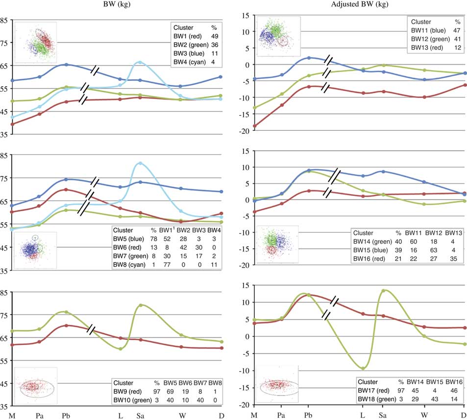
Cluster analysis highlighted four clusters for production cycles 1 and 2 for BW whereas three clusters were found for adjusted BW. Two clusters were observed for BW and adjusted BW at cycle 3 (Figure 1) with 95% to 100% of variances explained by the two or three first PC of FPCA, for adjusted BW and BW, respectively (data not shown).
Cluster profiles for BW (on the left) and adjusted BW (on the right) in Romane ewes over their over the production cycles 1 (at the top), 2 (in the middle) and 3 (at the bottom). The scatter plots appearing on the left of each graph represents the individual coordinates on the two first principal components of the functional principal component analysis. The textbox on the right of each graph indicates the proportion of animals present in each cluster, and is given in percentage (%). The composition of each cluster at productive cycle n is given by indicating the proportion (%) of animals from clusters found at previous cycle n−1. M = mating; Pa = early pregnancy; Pb = mid-pregnancy; L = lambing; Sa = beginning of suckling; W = weaning; D = dry-off; Adjusted BW = BW taking into account average individual BW levels across cycles.

For BW at production cycles 1 and 2, the two major clusters for each cycle together included 85% and 91% of the ewes, respectively (clusters BW1, BW2 and BW5 and BW6). For adjusted BW at cycles 1 and 2, the two major clusters included 88% of the ewes (clusters BW11 and BW12) and 79% of the ewes (clusters BW14 and BW14), respectively. Cluster BW1 showed a BW gain from BW-M to BW-Sa and a stabilized BW from BW-Sa to the end of cycle 1. Clusters BW2 and BW3 showed similar profiles but ewes in cluster BW3 were heavier than ewes in cluster BW2. The BW2 and BW3 profiles were similar to BW1 from BW-M to BW-Pb, and were characterized by a decrease in BW from the end of pregnancy to BW-W and then an increase until the end of cycle 1. Ewes in BW2 were heavier than ewes in cluster BW1 until BW-Sa and then had the same BW until BW-W. Cluster BW11 showed a similar profile to BW2 and BW3. Cluster BW12 showed a combination of BW1 and BW4 profiles characterized by a progressive increase in BW from mating to beginning of suckling and a slight decrease thereafter. Cluster BW13 showed a similar profile to BW11 but with a greater increase of BW between BW-W and BW-D. For cycle 2, clusters BW5 and BW7 showed parallel profiles and were similar to cluster BW3 in cycle 1 except for a slight increase in BW from BW-L to BW-Sa and a slight decrease from BW-Sa to BW-D. Cluster BW6 showed a similar profile to cluster BW3 in cycle1 but a marked decrease in BW between BW-Pb and BW-W. Ewes in cluster BW5 were heavier than in cluster BW7, as were the ewes in BW6 compared to those in cluster BW7, except at BW-W when the ewes had a similar BW value. Cluster BW14 had a similar profile to BW6 with a slighter increase at the end of the cycle. Cluster BW15 showed a similar profile to BW5 but with a higher decrease at the end of the cycle. Cluster BW16 had a similar profile to BW7 but showed a more stable profile between BW-Sa and BW-D. Clusters BW9 and BW17 included 97% of the ewes measured for cycle 3 and showed a similar profile to clusters BW5, BW7 and BW14 in cycle 2 but with either lower BW values than BW5 (i.e. BW) or similar range of variation than BW14 (i.e. adjusted BW). Clusters BW4, BW8, BW10 and BW18 for cycles 1, 2 and 3, respectively, were different from the other clusters with a marked increase of BW at BW-Sa, with a gain of 10, 16, 18 and 23 kg, respectively, to finally reach higher levels than those measured in the other clusters. This increase was followed by a marked decrease between BW-Sa and BW-W with a final BW close to that of the other clusters.
Generally, the ewes in each cluster originated from different clusters in the previous cycle but some constancy was observed. For example, the ewes in the BW5 cluster of cycle 2 originated mostly from clusters BW1 (52%) and BW2 (28%) of cycle 1. The ewes belonging to BW2 and BW5 also belonged to BW9 and exhibited almost the same profiles at cycles 1, 2 and 3. The majority of the ewes in cluster BW6 originated from clusters BW2 (42%) and BW3 (30%) of cycle 1 (Figure 1). These ewes also belonged to BW9 and exhibited almost the same profiles at cycles 1, 2 and 3. The majority of the ewes in cluster BW14 originated mostly from cluster BW11 (60%), whereas ewes in cluster BW15 originated from cluster BW12 (63%). Most of the ewes that belonged to BW11 and BW14 also belonged to BW17 at cycle 3 and showed similar profile along the three production cycles.
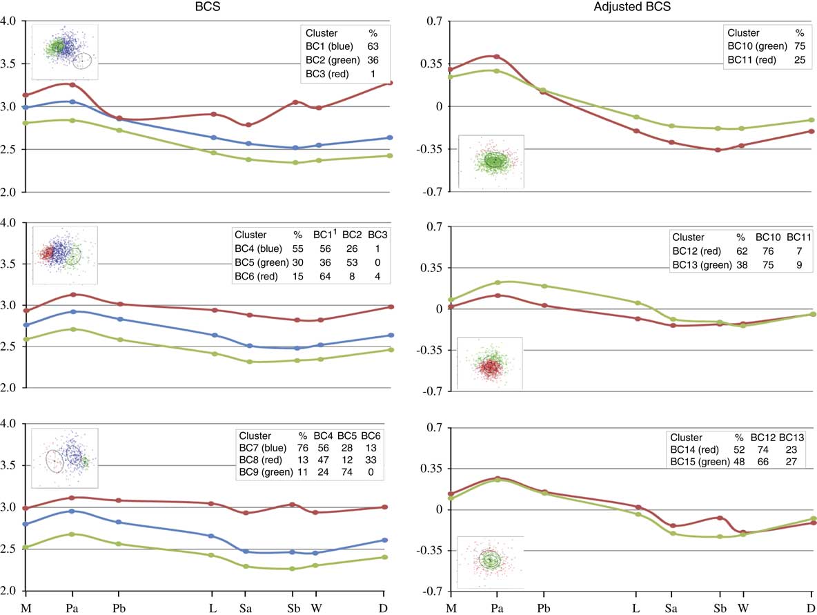
Cluster analysis of BCS in the whole population highlighted three clusters for each production cycle (Figure 2) with 98% to 100% of variances explained by the two or three first PC of FPCA, for adjusted BCS and BCS, respectively (data not shown). Cluster analysis of adjusted BCS highlighted two clusters for each production cycle (Figure 2) with 86% to 90% of variances explained by the two first PC of FPCA. During production cycles 1 and 2 for BCS, the two major clusters for each cycle included 99% and 85% of the ewes, respectively (clusters BC1, BC2 and BC4, BC5, respectively). In production cycle 3, the major cluster (BC7) included 76% of ewes. For adjusted BCS at cycles 1 and 2, the major cluster included 75% and 62% of the ewes (BC10 and BC12, respectively) and for cycle 3, ewes were distributed equally in the two clusters. Clusters BC1, BC2, BC4, BC5, BC6, BC7 and BC9 showed parallel within- and between-cycle profiles but different levels of BCS. The profiles for these clusters were characterized by an increase in BCS from BCS-M to BCS-Pa, a constant decrease from BCS-Pa to BCS-Sb and a progressive increase from BCS-Sb to the end of the production cycle. In cycle 3, cluster BC8 differed from clusters BC7 and BC9 by a very slight decrease of BCS between BCS-Pa and BCS-W and the highest BCS levels. Clusters for adjusted BCS showed very close ranges of variation within- and between-cycle and similar profiles to the main clusters found for BCS.
Cluster profiles for body condition score (BCS) (on the left) and adjusted BCS (on the right) in Romane ewes over their production cycles 1 (at the top), 2 (in the middle) and 3 (at the bottom). The scatter plot on the left of each graph represents the individual coordinates on the two first principal components of the functional principal component analysis. The textbox on the right of each graph indicates the proportion of animals in each cluster, which is given in percentage (%). The composition of each cluster at productive cycle n is given by indicating the proportion (%) of animals from clusters found at previous cycle n−1. BC = body condition; M = mating; Pa = early pregnancy; Pb = mid-pregnancy; L = lambing; Sa = beginning of suckling; Sb = end of suckling; W = weaning; D = dry-off; Adjusted BCS = BCS taking into account average individual BCS levels across cycles.

Ewes in cluster BC4 of cycle 2 originated mostly from clusters BC1 and BC2 (56% and 26%, respectively) of cycle 1. Ewes included in BC5 originated mainly from BC2 (53%) and BC1 (36%) of cycle 1. Ewes in BC6 originated mostly from BC1 (64%) of cycle 1, and ewes in BC7 from BC4 (56%) and BC5 (28%) of the previous cycle. Ewes in clusters BC12 and BC13 originated mostly from BC10 (76% and 75%, respectively). Ewes in cluster BC8 originated mainly from BC4 (47%) and BC6 (33%) of cycle 2 and those in cluster BC9 mainly from BC5 (74%) of cycle 2. Ewes in clusters BC14 and BC15 originated mostly from BC12 (74% and 66%, respectively). In general, these ewes exhibited the same profiles at cycles 1, 2 and 3.
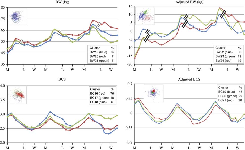
Figure 3 displays clusters observed considering ewes’ BW and BCS over their first three productive cycles. Three clusters were found for each trait. Considering BW clusters, the three profiles showed similar and parallel profiles over the three cycles. The main cluster included 87% of ewes and indicated that majority of ewes were globally gaining weight until the end of cycle 3 concomitantly with the observed alternation of weight gain and loss through each cycle. The two other clusters differed from the major one mainly at cycle 3 by higher or lower BW levels. Considering adjusted BW clusters, two of them (i.e. BW22 and BW24) showed similar and parallel profiles over the three cycles but with a crossing point between both trajectories during the second suckling period. The third cluster (i.e. BW23) differed from the two others in the alternation of weight gain and loss within- and between cycles. Considering BCS clusters, the main cluster (i.e. BC16, 76% of ewes) showed repeatable BCS gains and losses across the three first cycles while the two other clusters exhibited BCS gains and losses changing between cycles. Concerning adjusted BCS, the three clusters showed very close or overlapping trajectories and repeatable over the three cycles.
Cluster profiles for BW (at the top left), adjusted BW (at the top right), body condition score (BCS) (at the bottom left) and adjusted BCS (at the bottom right) over the entire productive life of Romane ewes. The scatter plot on the left of each graph represents the individual coordinates on the two first principal components of the functional principal component analysis. The textbox on the right of each graph indicates the proportion of animals in each cluster, which is given in percentage. BC = body condition; M = mating; L = lambing; W = weaning; Adjusted BW = BW taking into account average individual BW levels across cycles; Adjusted BCS = BCS taking into account average individual BCS levels across cycles.

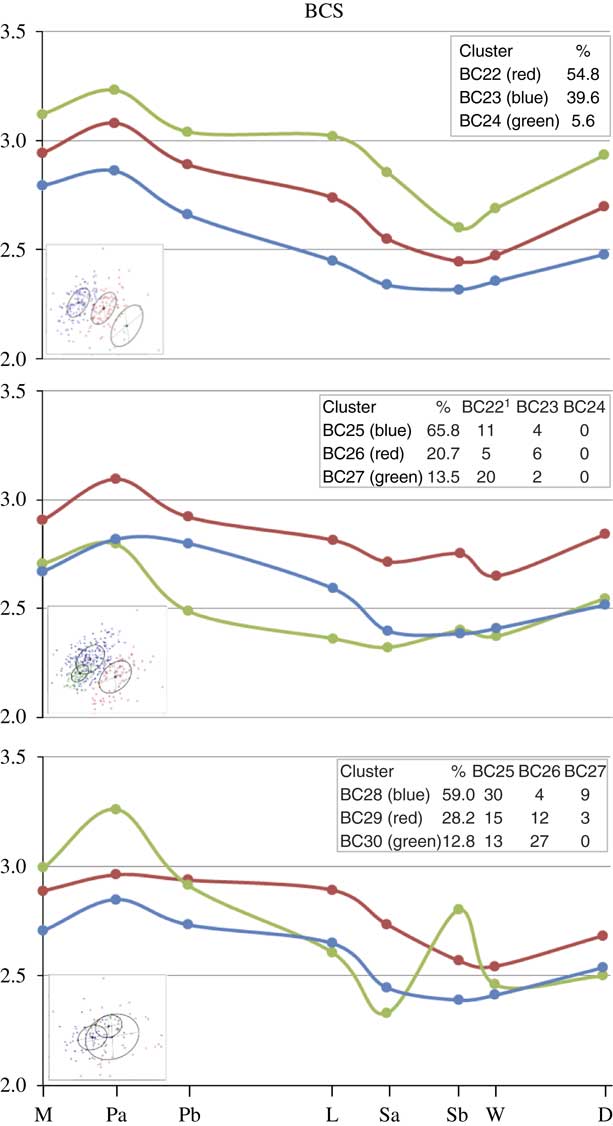
Figure 4 displays the BCS clusters observed considering only ewes lambing and suckling twins (no difference in the average age at first lambing between clusters within a cycle). Three clusters were identified for each production cycle. The two main profiles for each production cycle showed similar, parallel profiles, both within and between the cycles. The profiles were similar to those described for BCS clusters for the whole population. The two main clusters in cycles 1, 2 and 3 included 94.4%, 86.5% and 87.2% of ewes, respectively. There was 12% of the multiparous ewes that remained in clusters showing the highest BCS levels between cycles 2 and 3 (BC26 and BC29, respectively). Concerning the adjusted BCS for ewes lambing and suckling twins, only one trajectory was observed at cycles 1 and 3 and two trajectories at cycle 2 (data not shown), that presented the same profiles as the trajectories of the adjusted BCS (Figure 2).
Cluster profiles for body condition score (BCS) of Romane ewes lambing and suckling twins (Litter 3) over their production cycles 1 (at the top), 2 (in the middle) and 3 (at the bottom). The scatter plot on the left of each graph represents the individual coordinates on the two first principal components of the functional principal component analysis. The textbox on the right of each graph indicates the proportion of animals in each cluster, which is given in percentage (%). The composition of each cluster at productive cycle n is given by indicating the proportion (%) of animals from clusters found at previous cycle n−1. BC = body condition; M = mating; Pa = early pregnancy; Pb = mid-pregnancy; L = lambing; Sa = beginning of suckling; Sb = end of suckling; W = weaning; D = dry-off.

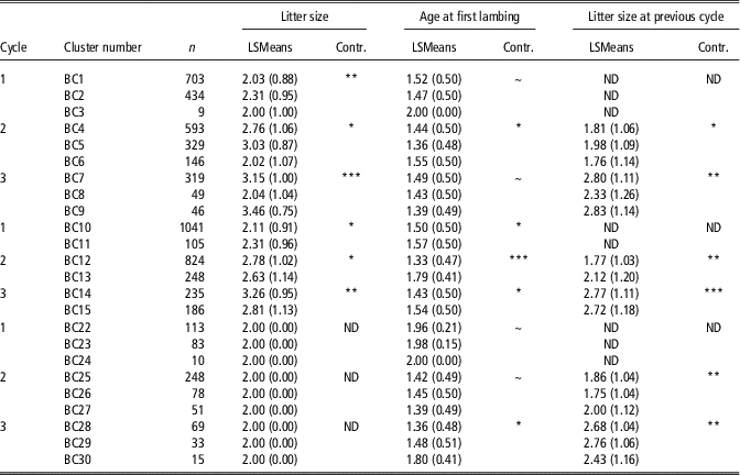
Biological factors
The main biological factors were tested to explain the distribution of the ewes between the clusters at each cycle (Tables 2 and 3). The Litter effect was the most significant effect for BCS clusters in the three production cycles. Ewes with the smallest average litter size were mostly included in clusters BC3, BC6 and BC8 that showed the highest BCS levels (Table 2). Ewes with larger litter sizes were included in clusters BC2, BC5 and BC9 that showed the lowest BCS in cycles 1, 2 and 3. When considering the adjusted BCS, all the variation factors (i.e. litter size, litter at previous cycle, age at first lambing and year) had similar effects on the trait. Ewes with larger litter sizes were included in clusters BC11, BC12 and BC14 that showed lowest BCS levels. Concerning BW and adjusted BW, ewes with the smallest average litter size were included in clusters BW1 and BW12 for cycle 1, BW5, BW7 and BW16 for cycle 2 and BW10 and BW18 for cycle 3 (Table 3).
Least-square (LS) means (±standard error) for litter size, age at first lambing and litter size at previous cycle for ewes present in each cluster of body condition score (BCS) at each production cycle

n = number of ewes; ND = non-determined; Contr. = contribution of the effect to the model based on Akaike information criteria and Bayesian information criteria: ~, *, **, ***indicate no, low, medium and high significant contribution of the effect to the model; BC1 to BC9 = BCS clusters; BC10 to BC15 = adjusted BCS clusters (i.e. BCS taking into account average individual BCS levels across cycles); BC22 to BC30 = BCS clusters for the subgroup of ewes lambing and suckling twins.
Least-square (LS) means (±standard error) for litter size, age at first lambing and litter size at previous cycle for ewes present in each cluster of BW at each production cycle

n = number of ewes; LSMeans = Least-square means; ND = non-determined; Contr. = contribution of the effect to the model based on Akaike information criteria and Bayesian information criteria: *, **, ***indicate no, low, medium and high significant contribution of the effect to the model; BW1 to BW10 = BW clusters; BW11 to BW18 = adjusted BW clusters (i.e. BW taking into account average individual BW levels across cycles).
Litter size at previous cycle had significant effect on ewes’ distribution in adjusted BCS clusters at cycle 2. Ewes that had a bigger litter size at cycle 1 were included in cluster BC12 showing lower BCS level. Considering BCS, litter size at previous cycle had very little effect at cycles 2 and 3 (Table 2). For adjusted BW, the ewes with the biggest litter size at previous cycle were included in clusters BW14 and BW17 showing progressive decrease in BW between mid-pregnancy and weaning. Considering BW, litter size at previous cycle had a significant and important effect. Ewes with bigger litter size at the previous cycle were included in clusters BW6 and BW9 at cycles 2 and 3, respectively, showing progressive decrease in BW between mid-pregnancy and weaning (Table 3).
The age of the ewe was the most significant effect for BW clusters at cycle 1, ranked second for BCS clusters at cycles 2 and 3 and was observed to be the less significant effect for BCS clusters at cycle 1 and BW clusters at cycles 2 and 3. For BCS at cycle 1, ewes that lambed at 1 year of age were included in clusters BC1 and BC2 and there were no differences in the age at first lambing for adjusted BCS at cycle 1. For the two other production cycles, the age at first lambing did not discriminate the clusters for BCS whereas, for adjusted BCS at cycle 2, ewes that lambed at 1 year of age were mostly included in BC12 (Table 2). For BW and adjusted BW at cycle 1, ewes that lambed at 1 year of age were included in clusters BW1, BW4, BW12 and BW13. For cycle 2, ewes that lambed at 1 year of age were included in BW8, BW15 and BW16 and the age at first lambing was not discriminating at cycle 3 (Table 3).
Discussion
The dynamics of body reserves as a trait for robustness in the current context
The accepted concept of ‘breeding for robustness’ (Kitano, Reference Kitano2004; Klopcic et al., Reference Klopcic, Reents, Philipsson and Kuipers2009; Molotsi et al., Reference Molotsi, Dube, Oosting, Marandure, Mapiye, Cloete and Dzama2017) justifies the necessity for gathering new insights into such traits in order to reveal the degree of individual robustness and the underlying determinant mechanisms (De La Torre et al., Reference De La Torre, Recoules, Blanc, Ortigues-Marty, D’Hour and Agabriel2015; Friggens et al., Reference Friggens, Blanc, Berry and Puillet2017). The BR dynamics have been shown to be a relevant trait for studying the capacity to overcome negative energy balance periods (Bauman and Currie, Reference Bauman and Currie1980; Nielsen et al., Reference Nielsen, Friggens, Løvendahl, Jensen and Ingvartsen2003; González-García et al., Reference González-García, Gozzo de Figuereido, Foulquie, Jousserand, Autran, Camous, Tesniere, Bocquier and Jouven2014). This trait is being considered as an interesting biological component in the design of future livestock systems (Dumont et al., Reference Dumont, González-García, Thomas, Fortun-Lamothe, Ducrot, Dourmad and Tichit2014; Phocas et al., Reference Phocas, Belloc, Bidanel, Delaby, Dourmad, Dumont, Ezanno, Fortun-Lamothe, Foucras, Frappat, González-García, Hazard, Larzul, Lubac, Mignon-Grasteau, Moreno, Tixier-Boichard and Brochard2016).
Relevance of BW and body condition score for interpreting body reserves dynamics
The BW and BCS are considered to be typical and relatively easily monitored parameters (Brown et al., Reference Brown, Savage, Hinch and Hatcher2015), and are usually analyzed to describe BR dynamics (Thorup et al., Reference Thorup, Edwards and Friggens2012; Morel et al., Reference Morel, Schreurs, Corner-Thomas, Greer, Jenkinson, Ridler and Kenyon2016; Puillet and Martin, Reference Puillet and Martin2017). Nevertheless, there is a consensus about the subjectivity of BCS due to disagreements about the methods used and inconsistent intra- and inter-operator assessment skills (Russel et al., Reference Russel, Doney and Gunn1969; Edmonson et al., Reference Edmonson, Lean, Weaver, Farver and Webster1989; Kenyon et al., Reference Kenyon, Maloney and Blache2014). One advantage of this study is the consistent assessment by the same two operators over the whole study period, with operators regularly attending training sessions to homogenize their scoring technique.
The main originality of our study was that we characterized the variability of existing BR dynamics profiles and described sequential and temporal BR changes, using longitudinal data covering up to three production cycles in a flock of ewes reared in extensive conditions. To our knowledge, this is the first report of longitudinal BR dynamics in several production cycles using real data, at least in grazing sheep.
Overall body reserves mobilization and accretion profiles
Both BW and BCS vary as an ewe progresses through the different physiological stages of the production cycle. The BRs are mobilized from mid-pregnancy until the end of the suckling period and this is reflected by a decrease in the BCS. After weaning, an increase in the BCS is observed (i.e. BR accretion) and lasts until the beginning of the next pregnancy. The BW and BCS profiles observed in our study population and conditions are consistent with the previously described overall dynamics (González-García et al., Reference González-García, Gozzo de Figuereido, Foulquie, Jousserand, Autran, Camous, Tesniere, Bocquier and Jouven2014). The simultaneous increase in BW and decrease in BCS observed between early to mid-pregnancy are likely to be due to the start of the fetus growth and development and the related increasing demand in energy (Bauman and Currie, Reference Bauman and Currie1980). The BW probably continued to increase during the second half of pregnancy but a BW measurement before lambing was missing in the present study to show the expected BW increase (González-García et al., Reference González-García, Gozzo de Figuereido, Foulquie, Jousserand, Autran, Camous, Tesniere, Bocquier and Jouven2014). This biased the tendency observed for BW between mid-pregnancy and lambing (Figure 1; missing point between mid-pregnancy – Pb- and lambing – L-).
During the 1st month of suckling, the decrease in BCS was probably due to an imbalance between energy intake and expenditure caused by the peak of milk production, a high priority given to the new-born lambs and the incapacity of the female to take in enough feed to meet energy requirements (Nielsen et al., Reference Nielsen, Friggens, Løvendahl, Jensen and Ingvartsen2003; Smith et al., Reference Smith, Friggens, Ashworth and Chagunda2017). The decreases in BCS and BW were observed despite the use of fertilized paddocks with enough quality biomass available to ensure the nutritional balance during the suckling period (Molénat et al., Reference Molénat, Foulquie, Autran, Bouix, Hubert, Jacquin and Bibe2005). An additional BCS measurement during the 2nd month of suckling could perhaps help to identify the exact endpoint of BR mobilization during this period.
The BW and BCS gains started again before the end of suckling. The stabilization or increase in BCS at this point could be related to a decrease in the ewes’ energy requirements and dietary diversification in lambs. This is consistent with the findings of another study (Kharrat and Bocquier, Reference Kharrat and Bocquier2010) that reported that BR replenishment was prioritized at the end of suckling in goats. Accretion continued during the autumn when ewes grazed the new herbage regrowth available in the native paddocks. It lasted during the dry-off period and until the beginning of the next pregnancy, including feed supplementation at mid-pregnancy (González-García et al., Reference González-García, Gozzo de Figuereido, Foulquie, Jousserand, Autran, Camous, Tesniere, Bocquier and Jouven2014).
In addition to the physiological stages of the production cycle, various biological factors such as parity, age at first parity, litter size or litter size at previous cycle had a significant impact on the BW and BCS levels of the females included in this study, as previously reported (María and Ascaso, Reference María and Ascaso1999; González-García et al., Reference González-García, Gozzo de Figuereido, Foulquie, Jousserand, Autran, Camous, Tesniere, Bocquier and Jouven2014 and Reference González-García, Tesniere, Camous, Bocquier, Barillet and Hassoun2015). A strong effect of litter size on BW loss was observed with the biggest litter sizes, since litter sizes were highly correlated between cycles, the BW loss may be related to two consecutive big litter sizes. The year/season also affected BR levels in our grazing system because the nutritional and energy balance are dependent on the weather and amount of biomass available.
Diversity of body reserves and body condition score profiles (cluster analysis)
In this study, we confirmed our hypothesis regarding the existence of different BW and BCS trajectories within a flock of Romane sheep reared in extensive conditions. Indeed, the characterization of variability in BCS profiles highlighted three separate trajectories for each production cycle. Most trajectories exhibited similar shapes (i.e. similar sequences of BCS gains and losses) but differed in terms of BW and BCS levels. This is confirmed by the two close trajectories observed with BCS taking into account average individual BCS levels across cycles (i.e. adjusted BCS). Indeed, trajectories found for adjusted BCS did not differ in the levels within cycle but slightly in the shape. Consideration of the average individual level across cycles did not highlight strong differences of trajectory. Some trajectories, essentially those showing the highest BCS levels, displayed different dynamics in addition to different BCS levels. The latter trajectories represented generally clusters including a lower number of animals. In addition, all BCS and adjusted BCS trajectories, whatever the production cycle, also suggested that BR accretion occurred from weaning to the next early pregnancy as described for overall BR profiles. The BR accretion during the dry-off period was associated with a stabilization or slight increase in BW depending on the various trajectories and production cycle. Consistently with the increase of BCS observed during early pregnancy, all BW and adjusted BW trajectories showed an increase in BW at this phase and later during pregnancy as hypothesized for the overall profile. While some BW trajectories differed only in the levels and not in the shape, these trajectories were not found for BW taking into account average individual BW level across cycles (i.e. adjusted BW). Thus, differences in the shape of adjusted BW profiles suggested that various BW trajectories existed within flock. In addition, BCS trajectories showing similar shape exhibited higher amplitude of BCS variation in primiparous ewes than in multiparous ewes. This suggest that improved efficiency in the use of BR could occur with time as the animal gains in ‘biological experience’.
The distribution of individual ewes between BCS and BW trajectories from one cycle to another was partially maintained. Between one-third and half of the ewes included in the biggest clusters remained in the same trajectory at the next cycle or even during the three cycles for BW, adjusted BW, BCS and adjusted BCS. Changes in the distribution of ewes between BCS trajectories in successive cycles are also probably related to changes in litter sizes. Indeed, the trajectory showing the highest BCS for each cycle included ewes with the smallest litter size, and conversely the trajectories with the low BCS levels included ewes with the largest average litter sizes. Nevertheless, ewes with similar litter size were also distributed in clusters showing different trajectories. This suggests that litter size, even if it was one of the most significant effect, was not the only factor explaining the distribution of ewes’ trajectories in this study. In addition, individual variability in BCS management may contribute to how ewes are distributed between the trajectories. Indeed, considering cluster analysis for BCS specifically in ewes lambing and suckling twins, three well-defined trajectories were also described for primiparous or multiparous ewes. Those trajectories differed by the level of BCS and/or the shape while clusters did not differ in litter size and age at first lambing. This was in accordance with the trajectories of ewes lambing and suckling twins obtained with the adjusted BCS (data not shown), which differed mainly in the shape. These results support the hypothesis of individual variability that contributes to BR dynamics whatever the litter size, parity or age at first lambing. Recent genetic studies considering BW and BCS changes over time supported the hypothesis of genetic determinism for weight and fat changes across production cycle (Macé et al., Reference Macé, González-García, Pradel, Parisot, Carrière, Douls, Foulquié and Hazard2018b; Walkom et al., Reference Walkom, Brien, Hebart, Fogarty, Hatcher and Pitchford2014).
Depending on trajectories and cycle, ewes recovered or increased their initial BW (i.e. at the beginning of cycle) at the end of the cycle. The variations in BW observed during the cycle resulted in few overall changes in BW between the beginning and the end of the cycle. Nevertheless, two BW trajectories and adjusted BW trajectories for production cycle 1 showed overall higher BW gain and represented 53% of the primiparous ewes, either considering BW or adjusted BW. The females included in these trajectories were the youngest ewes, so we hypothesized that these females were still growing, as previously reported by González-García and Hazard (Reference González-García and Hazard2016). Interestingly, when cluster analysis was performed for the ewes’ entire productive life, the BW trajectory including most of the ewes (i.e. 87%) suggested that females kept growing during their three first cycles. Trajectories were even better defined when taking into account average BW level across cycles since the ewes in the three adjusted BW trajectories kept gaining weight across the first cycles, despite alternating periods of BW gain and loss. Moreover, the youngest ewes at first lambing were ewes that gained the higher amount of BW across the three cycles. This is in accordance with the study of Zygoyiannis et al. (Reference Zygoyiannis, Stamataris, Friggens, Doney and Emmans1997) reporting growth in Greek ewes until they reached 3.5 years of age. It would be interesting to analyze BW trajectories in older ewes to determine at which age Romane ewes actually stop growing in this environment.
Our ‘ideal body reserves profile’ definition
When analyzing the diverse BW and BCS profiles found in our study, it seemed important to define what we deemed the ‘ideal profile’ of a robust ewe to be. Regarding BR dynamics efficiency, a robust ewe would be an individual that avoids quick and drastic losses in BRs when facing a negative energy balance challenge and reacts by quickly replenishing BRs to recover at least its initial status once the shortage ended without affecting its performance (Bocquier and González-García, Reference Bocquier and González-García2010; Martin and Sauvant, Reference Martin and Sauvant2010). Interestingly, cluster analysis for BCS in ewes with similar litter sizes still showed three clusters, as described in the whole population (Figure 4; Supplementary Figure S1). We hypothesized that the ‘robust trajectory’ was the trajectory that showed intermediate BCS levels in primiparous ewes (red profile; BC22) and the highest BCS in multiparous ewes lambing and suckling twins (profiles BC26 and BC29; Figure 3). Ewes belonging to the robust trajectory for all the three production cycles would be the most interesting ewes. For now, 5% to 12% of the ewes followed the robust trajectory for two cycles but none of them followed this trajectory for the three cycles.
To better characterize robust individuals, new parameters should be considered in addition to those evaluated here (BW and BCS). On the one hand, the longitudinal analysis of a set of plasma metabolites and hormones could provide additional, specific data on each individual’s energy metabolism. On the other hand, other zootechnical parameters related to the ewes’ reproductive and productive performances will be needed to define individual robustness in a multicriteria assessment approach. Everything as a whole would add to the quality of the ‘big-picture’ for a relevant interpretation of such a complex and multifactorial trait.
Conclusions
In this study, the analysis of the measurements recorded in the INRA historical database over several production cycles confirmed that BW and BCS levels in Romane ewes were, as expected, significantly affected by the age at first lambing, parity, physiological stage, litter size and litter size at the previous cycle, as well as by the year of measurement. Our most relevant findings are the identification of different profiles or trajectories for BCS and BW suggesting different dynamics in BR mobilization–accretion. For a proportion of the ewes, the profiles remained consistent throughout the animal’s life, whatever the age at first lambing, parity and litter size (i.e. repeatability of BR dynamics between successive cycles). Thus, the individual differences in profiles observed at a given stage illustrate the existence of proven intra-flock variability in the adaptive capacities of ewes to manage their BR. Such variability could probably be explained by a genetic component, which justifies further efforts to continue to explore the main genetic and physiological mechanisms behind this phenomenon.
Acknowledgments
The authors would like to thank the INRA Divisions of Animal Genetics and Animal Physiology and Livestock Systems for their financial support over the years in providing salaries, experimental costs and computational facilities. The authors are indebted to all the staff of ‘La Fage’ experimental farm for managing the experimental flock as well as for their active role in collecting experimental data.
Declaration of interest
The authors fully declare, under their responsibility, that there are no conflicts of interest to declare.
Ethics statement
The care and management of all animals whose BW and BCS measurements were included in this study was approved by the INRA’ Institutional and Regional Animal Care and Use Ethical Committee.
Software and data repository resources
None.
Supplementary materials
To view supplementary material for this article, please visit https://doi.org/10.1017/S175173111800352X