2. Experiment description

The experiments were conducted in a turbulent channel flow wind tunnel located at the University of Kentucky. This facility had a channel half-height of $h=50.8$  mm and could achieve area averaged velocity $U_{b}=30$  m s $^{-1}$ , resulting in Reynolds numbers up to $Re_{b}=2hU_{b}/{\it\nu}=1.9\times 10^{5}$ or $Re_{{\it\tau}}=hu_{{\it\tau}}/{\it\nu}=4000$ , where $u_{{\it\tau}}=({\it\tau}_{w}/{\it\rho})^{0.5}$ with ${\it\tau}_{w}$ the wall shear stress and ${\it\rho}$ the density. Air was driven through the channel using an in-line blower located at the inlet with the flow conditioned by a series of six flow conditioning screens and a 9:1 contraction before entering a channel section. The channel section had an aspect ratio of 9:1, expected to provide quasi-2-D flow at the centreline (Zanoun, Durst & Nagib Reference Zanoun, Durst and Nagib2003) and was equipped at the channel inlet with a boundary-layer trip consisting of a 50 mm wide section of 120 grit sand paper followed by a 100 mm wide section of 60 grit sandpaper. The distance from the channel inlet to the test location was $246h$ , allowing the turbulence to reach a fully developed state naturally (Monty Reference Monty2005) before entering the measurement section. This measurement section was $24h$ long and was equipped with an insert located at the centre of the upper surface for introducing instrumentation into the flow. Following the measurement section, an additional $12h$ long section isolated the measurement section from exit conditions. Surface roughness was measured on a sample of the measurement section wall using a stylus surface profilometer. The sample was found to have an r.m.s. roughness height of 268 nm along the grain of the aluminium and 334 nm across the grain, corresponding to 2.5 % of the viscous length scale at the highest Reynolds number reported here.

To determine the friction velocity, the channel facility was outfitted with static pressure taps every $12h$ along its length, which allowed determination of the pressure loss in the fully-developed section of the channel using a simple momentum balance (see, for example Pope Reference Pope2000). For this experiment, the nine pressure taps closest to the measurement section were measured by an array of 1000 Pa transducers. All transducers were calibrated before the experiment using a liquid manometer with $\pm$ 0.06 Pa accuracy.

Measurements of streamwise velocity, $U_{1}$ , were conducted over a range of wall-normal distances, $y=x_{2}$ , at $Re_{{\it\tau}}=490$ , 950, 2080 and 4100. At the lowest Reynolds number, these measurements were made using a conventional hot-wire probe constructed from platinum-core Wollaston wire etched to a sensing length of $\ell =0.50$  mm and diameter of 2.5  ${\rm\mu}$ m. The resulting $\ell ^{+}=\ell u_{{\it\tau}}/{\it\nu}<5$ with the maximum $\ell /{\it\eta}_{K}\approx 2$ occurring close to the wall. The probe was driven by a constant temperature anemometer (Dantec Streamline CTA) system at an overheat ratio of $1.6$ producing a measured square-wave frequency response of $f_{sw}=60$  kHz. The CTA signal was low pass filtered at 60 kHz using an analogue 4-pole Butterworth filter (Krohn-Hite model 34A) before being digitized at $f_{s}=200$  kHz by a 16-bit data acquisition system (National Instruments NI-PCI 6123).

To achieve the higher spatial and temporal resolutions required for the three higher Reynolds number cases, a nanoscale thermal anemometry probe (NSTAP) was used (Bailey & Smits Reference Bailey and Smits2010; Vallikivi & Smits Reference Vallikivi and Smits2014). These probes have been successfully employed in the measurement of turbulent wall-bounded flows at both low and high Reynolds numbers (Vallikivi et al. Reference Vallikivi, Hultmark, Bailey and Smits2011; Hultmark et al. Reference Hultmark, Vallikivi, Bailey and Smits2012, Reference Hultmark, Vallikivi, Bailey and Smits2013; Bailey et al. Reference Bailey, Vallikivi, Hultmark and Smits2014). The probe used in this study had a sensing element measuring 60  ${\rm\mu}$ m long $\times$ 2  ${\rm\mu}$ m wide $\times$ 100 nm thick, resulting in $\ell ^{+}=1,3$ and 5 with corresponding maximum $\ell /{\it\eta}_{K}\approx 0.4,1.1$ and 2.12. The NSTAP was operated in the same system as the conventional probe, although at a resistance overheat ratio of 1.2 which resulted in a square-wave frequency response of $f_{sw}=120$ , 160 and 111 kHz for $Re_{{\it\tau}}=950$ , 2080 and 4100, respectively. Corresponding low-pass filter frequencies were 100, 150 and 100 kHz and digitization frequencies were $f_{s}=200$ , 300 and 200 kHz.

Calibration of the probes took place in situ, directly prior to, and following, each measurement run using a Pitot probe located at the channel centreline. Static pressure was measured by two interconnected 1 mm diameter static taps located 25.4 mm apart, equidistant from the centre plane. To maximize sensitivity over the range of calibration velocities, the pressure difference between Pitot tube and static taps was measured simultaneously by four transducers having sensitivities of 12.5, 125, 750 and 1000 Pa. As with the static taps along the channel length, all transducers were calibrated before the experiment using a liquid manometer with $\pm$ 0.06 Pa accuracy. Air temperature was monitored by a thermistor probe located in the measurement section of the channel and CTA bridge voltages corrected in post-processing for any measured temperature drift (Tavoularis Reference Tavoularis2005). A fourth-order polynomial was used to fit the calibration curves which were used to convert the measured time dependent voltage into time series of $U_{1}$ .

To traverse the probes in the channel, a nano-stepping traverse equipped with a high-accuracy linear encoder was used (500 nm resolution and $\pm$ 3  ${\rm\mu}$ m accuracy). The relative position of the hot-wire relative to the wall was set using an electrical contact switch which triggered at the initial probe position for each measurement. The distance of the probe to the wall at this initial measurement location was determined with a distance measuring microscope with an accuracy of $\pm$ 5  ${\rm\mu}$ m (Titan Tool Supply ZDM-1) and was nominally 85  ${\rm\mu}$ m for the hot-wire probe and 50  ${\rm\mu}$ m for the NSTAP. Traverses were made with the number of measurement positions and sample times, $T_{s}$ , adjusted for each Reynolds number to ensure converged statistics for each case. Experimental conditions are summarized in table 1.

Table 1.

Experimental conditions.

3. Describing the large scales

Within this section we present the measured statistics traditionally used to describe the small scales and use these results to justify the need for a modified descriptor for $L$ in the local large-scale Reynolds number. As typically required for thermal anemometry (i.e. Meneveau & Sreenivasan Reference Meneveau and Sreenivasan1991), Taylor’s frozen flow hypothesis (Taylor Reference Taylor1938) was invoked in the calculation of all spatial statistics in order to translate temporal information into spatial information. Here, the local mean streamwise velocity was assumed to be the convective velocity of all turbulent scales such that ${\rm\Delta}x_{1}\approx \langle U_{1}\rangle {\rm\Delta}t$ . Although Taylor’s hypothesis is generally accepted to be a reasonable approximation for the smallest scales of turbulence, which are the focus of the current study, it is also well known to introduce error in translating the larger scale, long-wavelength motions from the temporal to spatial domain (i.e. Zaman & Hussain Reference Zaman and Hussain1981; del Álamo & Jiménez Reference del Álamo and Jiménez2009).

To estimate ${\it\eta}_{K}$ an estimate of $\langle {\it\varepsilon}\rangle$ must first be found. One approach is to assume local isotropy which allows $\langle {\it\varepsilon}\rangle$ to be determined from integration of the one-dimensional dissipation spectrum $D(k_{1})$ (Townsend Reference Townsend1976) such that

Here $D(k_{1})$ was, in turn, approximated using the longitudinal one-dimensional energy spectrum $E_{11}(k_{1})$ and the streamwise wavenumber found from Taylor’s hypothesis using $k_{1}\approx 2{\rm\pi}f/\langle U_{1}\rangle$ . Since the turbulence signals were oversampled in the present measurements, the integration cutoff $k_{c}$ was required to prevent contamination of the $\langle {\it\varepsilon}\rangle$ estimate by the $f^{2}$ noise of the anemometer (Saddoughi & Veeravalli Reference Saddoughi and Veeravalli1996). This cutoff wavenumber was selected using the frequency where an inflection appeared in the frequency spectrum. In other words, the frequency at which instrumentation noise was of the same order as the turbulent signal.

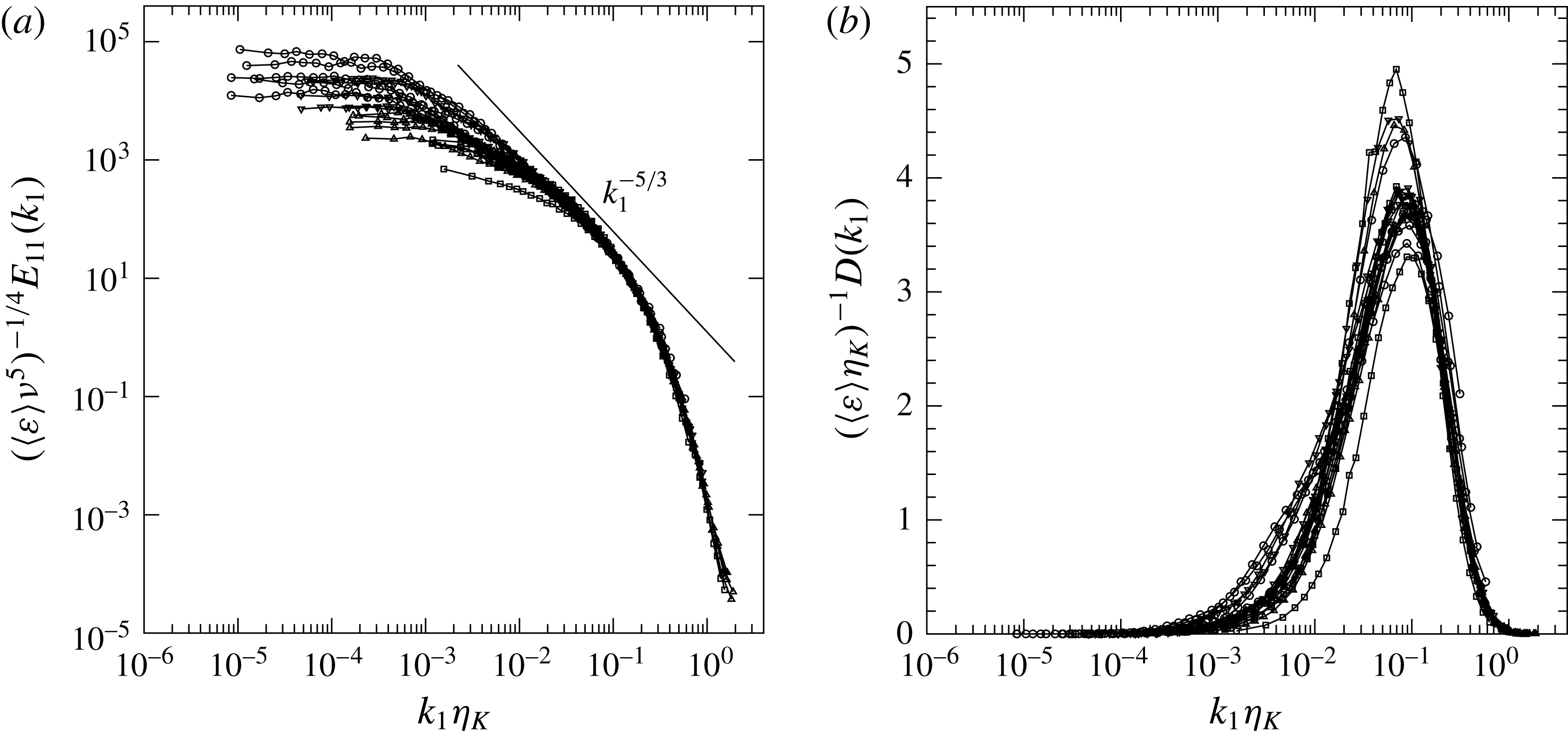
The measured longitudinal one-dimensional energy spectra are shown in figure 1(a) for several $y$ positions at each $Re_{{\it\tau}}$ with the corresponding one-dimensional dissipation spectra presented in figure 1(b). The spectra in figure 1(a) have been scaled using Kolmogorov scaling and, as expected, the scaled spectra collapse at large $k_{1}{\it\eta}_{K}$ . Note that, even at the highest $Re_{{\it\tau}}$ measured, there is little evidence of the existence of an appreciable inertial subrange. In addition, it was found that for $y^{+}=yu_{{\it\tau}}/{\it\nu}<30$ the collapse of the spectra degraded, which is believed to be due to a breakdown in the validity of the assumptions used to calculate $\langle {\it\varepsilon}\rangle$ . For this reason, results from $y^{+}<30$ are not included here.

Figure 1.

(a) Normalized longitudinal one-dimensional energy spectra measured at $y^{+}\approx 30$ and 100, and at $y/h=0.2,0.5$ and 1. (b) Corresponding estimate of the dissipation spectra. Symbols as in table 1.

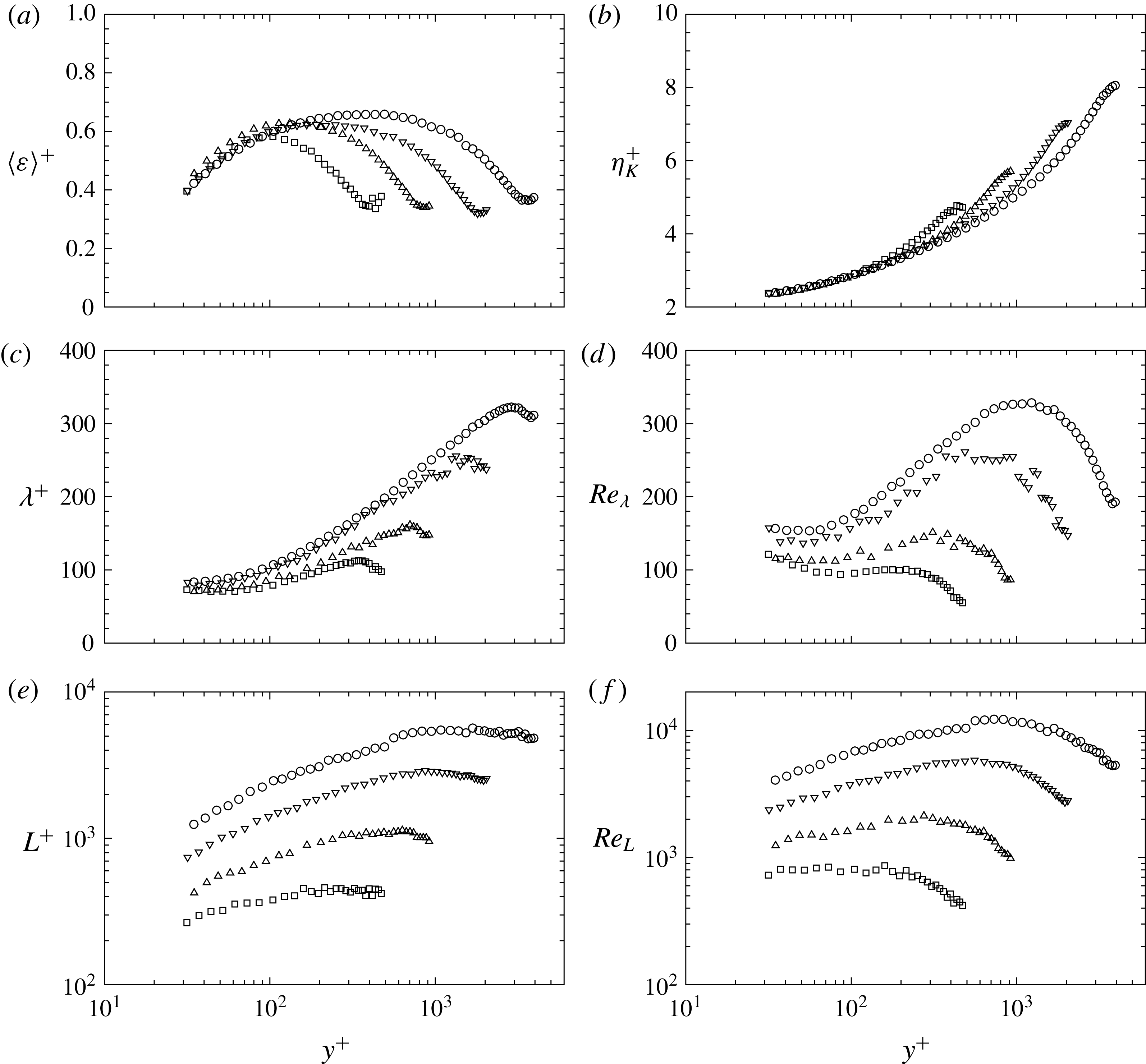
The wall normal distribution of inner-scaled dissipation $\langle {\it\varepsilon}\rangle ^{+}=\langle {\it\varepsilon}\rangle 0.4y/u_{{\it\tau}}^{3}$ is shown alongside the inner-scaled Kolmogorov scale ${\it\eta}_{K}^{+}={\it\eta}_{K}u_{{\it\tau}}/{\it\nu}$ in figure 2(a,b), respectively. In both cases, the inner-scaled profiles collapse within the range $y^{+}<0.2Re_{{\it\tau}}$ , consistent with the dependence of the small-scale properties within the inner layer being dependent only on wall shear stress and viscosity. The collapse within the range $y^{+}<100$ is particularly interesting, given the lack of Reynolds number scaling of the statistics of the large scales for this flow, as reflected, for example, in the growth in the near-wall peak in $\langle u_{1}^{2}\rangle ^{+}$ with $Re_{{\it\tau}}$ (i.e. as discussed in Marusic et al. Reference Marusic, McKeon, Monkewitz, Nagib, Smits and Sreenivasan2010), but is consistent with the scaling observed by Hutchins et al. (Reference Hutchins, Nickels, Marusic and Chong2009) in their high-pass filtered streamwise Reynolds stress.

Figure 2.

Wall normal dependence of: (a) mean dissipation rate; (b) Kolmogorov scale; (c) Taylor microscale; (d) Taylor Reynolds number; (e) integral length scale; and (f) large-scale Reynolds number. Symbols as in table 1.

Although the statistics describing the smallest scales follow inner scaling, Reynolds number dependence near the wall can be observed in the Taylor microscale, which here is estimated from

and shown as profiles of ${\it\lambda}_{f}^{+}={\it\lambda}_{f}u_{{\it\tau}}/{\it\nu}$ in figure 2(c). Given that ${\it\lambda}_{f}$ is a hybrid scale formed from a mix of large and small-scale statistics, it is not surprising that the Reynolds number dependence of the large-scale statistics is evident in ${\it\lambda}_{f}^{+}$ .

It is often convenient, particularly in homogeneous isotropic turbulence, to characterize the turbulence using the Taylor-scale Reynolds number

The wall-normal dependence of $Re_{{\it\lambda}}$ is provided in figure 2(d). Whereas at low $Re_{{\it\tau}}$ the maximum value of $Re_{{\it\lambda}}$ occurs near the wall at the location of the near-wall production cycle, as $Re_{{\it\tau}}$ increases a local maximum of $Re_{{\it\lambda}}$ develops in the outer layer near $y^{+}\approx 0.3Re_{{\it\tau}}$ . The increase of this outer peak with $Re_{{\it\tau}}$ outpaces the near-wall increase in $Re_{{\it\lambda}}$ with $Re_{{\it\tau}}$ . This reflects the increasing confinement in large scales as the near-wall production cycle moves closer to the wall. Thus, even though the turbulence intensity near the wall increases with $Re_{{\it\tau}}$ , the increase in turbulence Reynolds number is limited. Conversely, in the outer layer, the large scales remain $O(h)$ and the increase in turbulent kinetic energy production with increasing $Re_{{\it\tau}}$ results in a comparatively larger increase in $Re_{{\it\lambda}}$ compared to near the wall. Note that the non-monotonic wall-normal dependence of $Re_{{\it\lambda}}$ results in multiple wall-normal locations having identical $Re_{{\it\lambda}}$ at the same $Re_{{\it\tau}}$ .

The integral length scale is commonly used to describe the scale of the energy-containing eddies and is defined from the longitudinal autocorrelation. Here, Taylor’s hypothesis is used to find the integral length scale as

In practice, small experimental bias and precision errors often result in slow convergence of the integral, so the an upper bound of ${\it\tau}_{c}$ was applied. The criterion used here was that of integrating either to the first zero-crossing, or first inflection of the autocorrelation, whichever occurs at a lower value of ${\it\tau}$ .

The wall-normal dependence of $L^{+}=Lu_{{\it\tau}}/{\it\nu}$ is presented in figure 2(e) and is found to be $O(Re_{{\it\tau}})$ far from the wall, decreasing towards the wall. The corresponding values of $Re_{L}$ are shown in figure 2( f) and, as with $Re_{{\it\lambda}}$ , at a single $Re_{{\it\tau}}$ there exists multiple $y$ locations with the same value of $Re_{L}$ . To calculate $Re_{L}$ , the average velocity increment was estimated by time averaging $|{\it\delta}_{L}u|\approx |u_{1}(t+L/\langle U_{1}\rangle )-u_{1}(t)|$ for all $t$ .

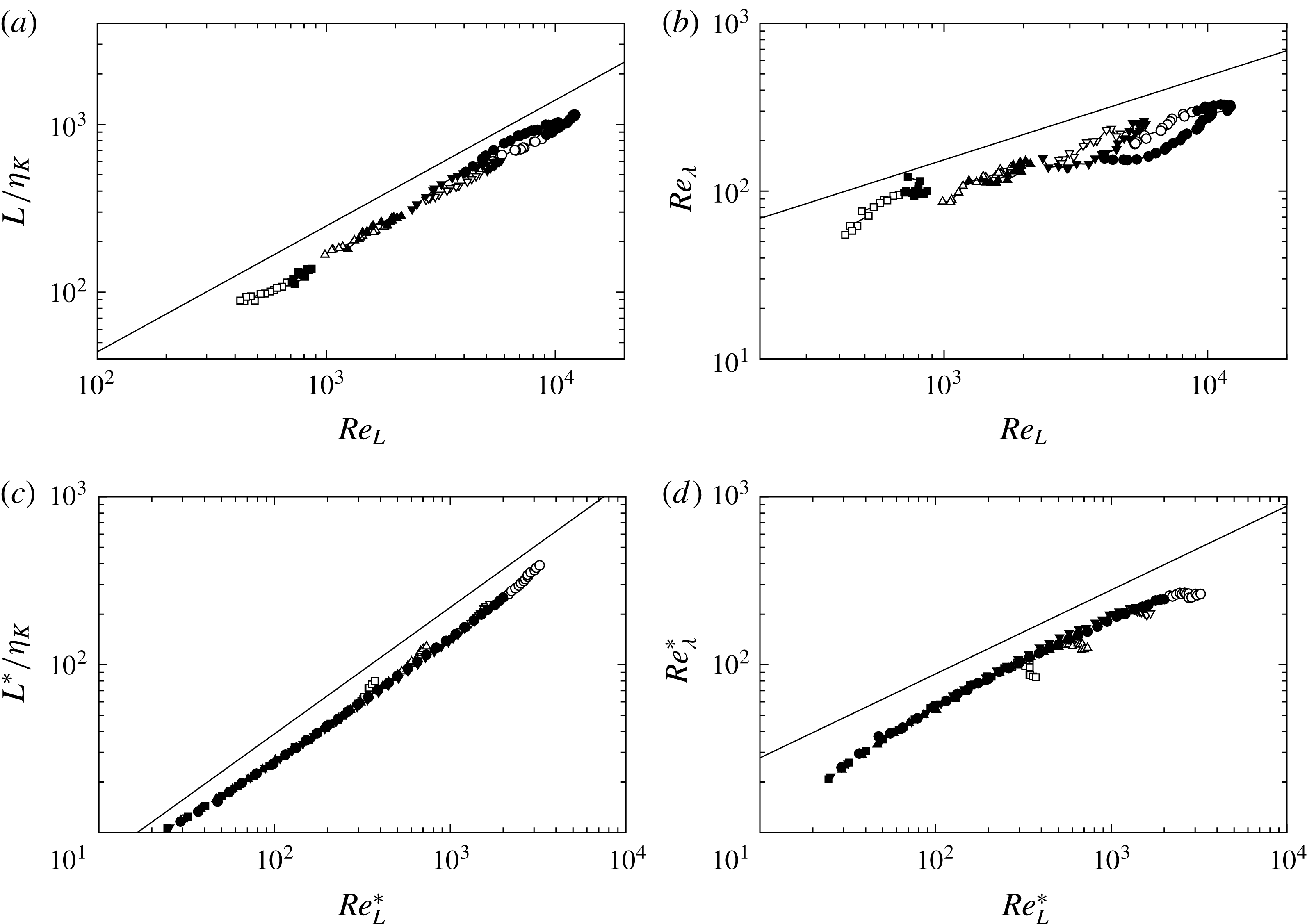
The non-monotonic wall-normal dependence of the statistics presented in figure 2 reveals the challenge of defining suitable Reynolds number scaling of the small-scale statistics. For example, classical theory suggests $L/{\it\eta}_{K}\sim Re_{L}^{0.75}$ and $Re_{{\it\lambda}}\sim Re_{L}^{0.5}$ (see, for example, Frisch Reference Frisch1995). Thus, one would expect $Re_{{\it\lambda}}$ to have the same value at a certain $Re_{L}$ , likewise for the ratio $L/{\it\eta}_{K}$ . However, as shown in figure 3(a,b), this is not the case. For both figure 3(a,b) the general trend agrees with the scaling predicted by classical theory. It is also clear that there is both $Re_{{\it\tau}}$ and $y$ influence within these trends. It is worthwhile noting that the $Re_{{\it\tau}}$ dependence is evident even at relatively high $y/h$ , where the large-scale anisotropy is weak and thus the lack of scaling cannot be attributed to anisotropy of the large scales.

Figure 3.

Dependence of (a) $L/{\it\eta}$ and (b) $Re_{{\it\lambda}}$ on $Re_{L}$ and dependence of (c) $L^{\ast }/{\it\eta}$ and (d) $Re_{{\it\lambda}}^{\ast }$ on $Re_{L}^{\ast }$ . Symbols as in table 1, solid symbols indicate measurement locations where $y/h<0.5$ .

In the phenomenological description of turbulence, the scale $L$ is intended to represent scales at the top of the inertial cascade and have nearly Gaussian statistics. However it is now understood that the large-scale structure of wall-bounded flow consists of several classes coherent motions. Such motions include the sublayer streaks observed by Kline et al. (Reference Kline, Reynolds, Schraub and Runstadler1967), hairpin vortices in the near-wall region (Head & Bandyopadhyay Reference Head and Bandyopadhyay1981), low wavenumber large-scale motions which have been associated with the occurrence of bulges of turbulent fluid at the edge of the wall layer (Kim & Adrian Reference Kim and Adrian1999; Guala, Hommema & Adrian Reference Guala, Hommema and Adrian2006; Balakumar & Adrian Reference Balakumar and Adrian2007) and meandering, very-large-scale motions or superstructures observed in the overlap region and, for pipes and channel flows, the wake region as well (Kim & Adrian Reference Kim and Adrian1999; Tomkins & Adrian Reference Tomkins and Adrian2005; Guala et al. Reference Guala, Hommema and Adrian2006; Balakumar & Adrian Reference Balakumar and Adrian2007; Hutchins & Marusic Reference Hutchins and Marusic2007; Monty et al. Reference Monty, Stewart, Williams and Chong2007, Reference Monty, Hutchins, Ng, Marusic and Chong2009). In addition, large-scale eddies far from the wall interact with smaller scales near the wall by introducing long wavelength velocity fluctuations through a modulation process (Mathis, Hutchins & Marusic Reference Mathis, Hutchins and Marusic2009).

Given the complex makeup of the energy containing motions, the integral scale will represent an amalgam of these multiple influences and bias towards longer motions, particularly near the wall, rather than accurately represent eddies with approximately Gaussian statistics at the top of the inertial cascade, as assumed in theoretical treatments (i.e. as done by Yakhot Reference Yakhot2006). Thus, it should not be surprising that use of the integral scale for defining $Re_{L}$ in channel flow is ineffective at capturing the same Reynolds number scaling observed in simpler flows.

Instead, we define a length-scale $L^{\ast }$ intended to describe the locally smallest energy-producing (i.e. active) eddies. Correspondingly we can define

and

where ${\it\delta}_{L}u^{\ast }$ is the longitudinal velocity increment, defined in (1.3), with $|\boldsymbol{r}|=L^{\ast }$ .

To find $L^{\ast }$ , we assume validity of Townsend’s attached eddy hypothesis, which states that Reynolds-stress-contributing eddies centred at $y$ are confined by the wall and therefore cannot have a scale larger than $y$ (Townsend Reference Townsend1976). We also note that Perry, Henbest & Chong (Reference Perry, Henbest and Chong1986) hypothesized that the energy containing range of the power spectrum will depend only on $u_{{\it\tau}}$ , $k_{1}$ , $y$ and $h$ given that eddies will only interact if their sizes are comparable. This leads to the assumption that non-local eddies of scale $h$ will contribute only to the low-wavenumber range of the spectrum for $y\ll h$ such that

and that, following the attached eddy hypothesis, the moderate to high wavenumber portion of the energy-containing range of the spectrum will consist of contributions from eddies scaling with $y$ such that

Although Perry et al. proposed that at sufficiently high Reynolds number an overlap region of validity would exist, leading to a $k_{1}^{-1}$ scaled subrange, experimental evidence provided by Morrison et al. (Reference Morrison, McKeon, Jiang and Smits2004) and Vallikivi, Ganapathisubramani & Smits (Reference Vallikivi, Ganapathisubramani and Smits2015), amongst others, find little support for this overlap region. However, these studies do demonstrate that within the turbulent wall region ( $y/h\lessapprox 0.15$ ) the low wavenumber portion of the spectrum scales with $h$ and the high wavenumber portion of the spectrum scales with $y$ , as predicted by (3.8) and (3.9). This suggests that the smallest energy-containing eddies, and thus the top of the inertial cascade, is composed of eddies which scale with $y$ . Note also that the largest possible isotropic eddies centred at a given $y$ will have a scale $\propto y$ .

We therefore assume that an appropriate length scale to describe the local, active contributions to the Reynolds stress, and upper bound of the inertial subrange, is one that is $\propto y$ for $y\ll h$ which leads to the definition of $L^{\ast }=0.8y$ . The constant of proportionality of 0.8 has no theoretical basis but was simply the value found to be most effective at non-dimensionalizing the dissipative motions for $y\lessapprox 0.5h$ . However, the results were found to be largely insensitive the constant selected with the greatest sensitivity found in the $y$ dependence of the local dissipation scales presented later in § 5.

It is therefore expected that $L^{\ast }$ will result in a value of local-large-scale Reynolds number representing local contributions to Reynolds stress that are free of the non-local, large-scale contributions to velocity fluctuations via amplitude modulation (referred to as ‘inactive’ eddies by Townsend) which cause $L$ near the wall to be of the same order as $h$ .

The improvement in scaling behaviour through the use of $L^{\ast }$ is demonstrated by the dependence of $L^{\ast }/{\it\eta}$ and $Re_{{\it\lambda}}^{\ast }$ on $Re_{L}^{\ast }$ as shown in figure 3(c,d), respectively. In both cases, the agreement with the classical theory is much improved for $y/h<0.5$ , with the $Re_{{\it\tau}}$ and $y$ influence on the turbulence parameters in this range captured by the revised description of the large scales. The resulting collapse of the results suggests that $Re_{L}^{\ast }$ is suitable for describing the Reynolds number dependence of the small-scale dissipative statistics in wall-bounded flow, at least for $y/h<0.5$ , where the attached eddy hypothesis can be assumed to be valid.

4. Moments of dissipation rate

As previously noted, through definition of dissipation as a fluctuating field, Yakhot (Reference Yakhot2006) arrived at (1.9) as a description for the Reynolds number dependence of the moments of the dissipation rate. This theory was tested by Schumacher (Reference Schumacher2007) using low-Reynolds-number DNS of homogeneous isotropic turbulence and again by Hamlington et al. (Reference Hamlington, Krasnov, Boeck and Schumacher2012) using DNS of turbulent channel flow. In both cases, good agreement was found with the theory. However, for turbulent channel flow, Hamlington et al. (Reference Hamlington, Krasnov, Boeck and Schumacher2012) observed that the moments of the dissipation rate exhibited both wall-normal dependence and $Re_{{\it\tau}}$ dependence, and thus only the Reynolds number dependence of the nearly isotropic centreline was used to evaluate the exponent $n$ . Therefore, it has yet to be demonstrated that the dissipation rate in the increasingly anisotropic turbulence for $y<h$ follows the predicted scaling.

As the thermal anemometry probe used in the present study was only capable of resolving the streamwise component of velocity, measurement of the all components of the time-dependent local rate-of-deformation tensor was not possible. Hence, the dissipation rate was calculated using the one-dimensional surrogate

As noted by Pope (Reference Pope2000) for example, such surrogates are only assumed to be qualitatively similar to the instantaneous dissipation. Here, to estimate this surrogate, Taylor’s hypothesis and a first-order finite difference were employed such that

with ${\rm\Delta}t=1/f_{s}$ . In the present case, to remove contamination from instrumentation noise, an additional zero-phase, eigth-order digital Butterworth filter was applied to the data with a cutoff frequency selected at the frequency at which the spectra is at a local minimum. Estimates of $\langle {\it\varepsilon}\rangle$ determined from both (3.1) and (4.2) were found to be in agreement, providing confidence in the implementation of (4.2).

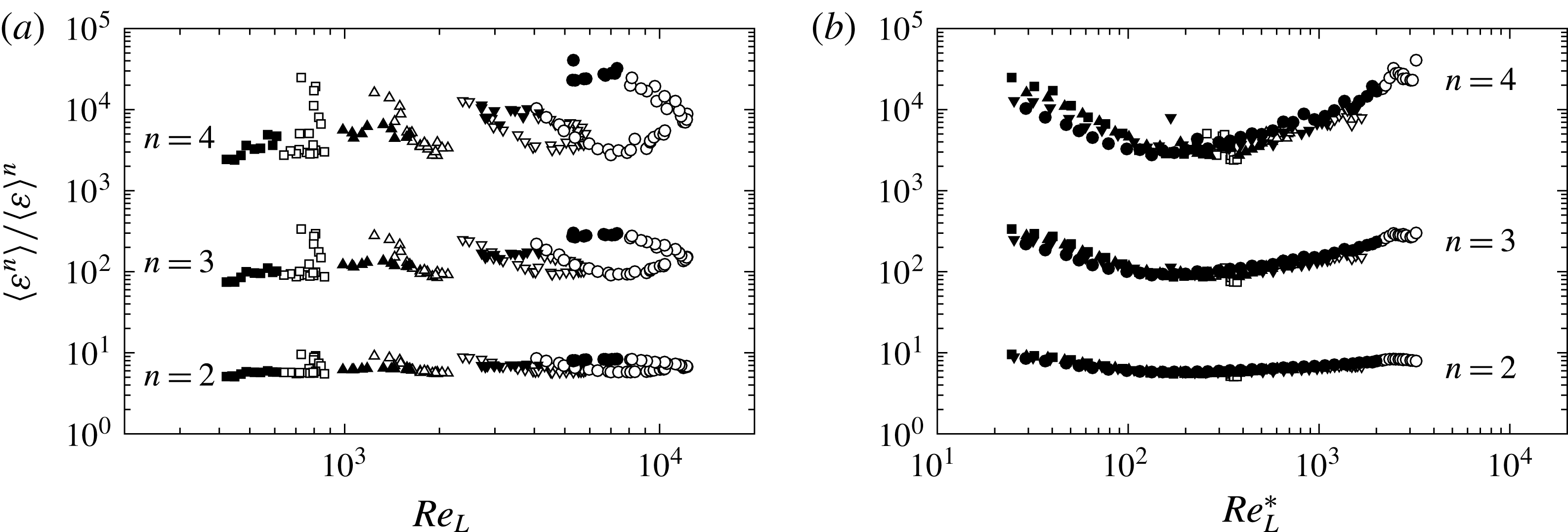
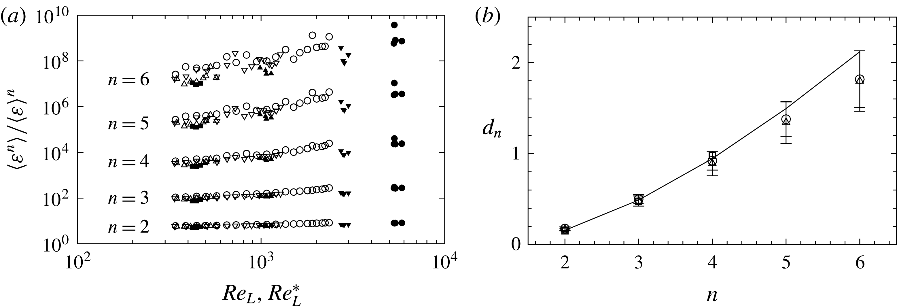
The Reynolds number dependence of the normalized dissipation moments $\langle {\it\varepsilon}^{n}\rangle /\langle {\it\varepsilon}\rangle ^{n}$ calculated from the time series determined from (4.2) is shown in figure 4 for $n=2$ –4. When the Reynolds number dependence is examined in terms of the local large-scale Reynolds number using the integral length scale, $Re_{L}$ , as is done in figure 4(a), there is no clear trend in the data, and the $Re_{{\it\tau}}$ and $y^{+}$ dependence observed in Hamlington et al. (Reference Hamlington, Krasnov, Boeck and Schumacher2012) is observed. There is also little support for the scaling described by (1.9) in these results.

Figure 4.

(a) Normalized dissipation moment. (b) Normalized dissipation moments. Symbols as in table 1 with solid symbols in (a) indicating measurement locations where $y>0.6h$ and solid symbols in (b) indicating measurement locations where $y<0.5h$ .

However, when the Reynolds number dependence of the dissipation moments is expressed using the local large-scale Reynolds number $Re_{L}^{\ast }$ , there is significantly improved collapse of the data amongst the results at different $y$ and $Re_{{\it\tau}}$ . For $Re_{L}^{\ast }\lessapprox 200$ the trend is reversed, suggesting insufficient separation between energy-containing and dissipative motions for (1.9) to be valid. Hamlington et al. (Reference Hamlington, Krasnov, Boeck and Schumacher2012) also observed a similar increase for their lowest Reynolds number case and attributed it to enhanced dissipation introduced by bursting of coherent structures. For $Re_{L}^{\ast }>200$ , the predicted power law behaviour can be observed, at least up to $y/h<0.8$ , which exceeds the limit at which $Re_{L}^{\ast }$ is expected to be a valid descriptor for the large scales. It is expected that as $y\rightarrow h$ , and the large-scale turbulence becomes increasingly isotropic, $L$ becomes a more suitable descriptor for the large scales. Indeed, as shown in figure 4(a) in which data points where $y>0.6h$ have been highlighted, far from the wall the dissipation moments appear to follow a power law scaling with $Re_{L}$ . This is coarsely analogous to the inner/outer scaling used to describe the Reynolds scaling of the mean flow and, to a lesser extent, the Reynolds stresses, however the ranges in which each form of scaling applies appears to be slightly different in the present case.

To quantitatively compare the Reynolds number dependence to the existing theory, the exponent $d_{n}$ was determined for $n=2$ –6 by separately fitting (1.9) for the range $Re_{L}^{\ast }>300$ and $y/h<0.6$ using $Re_{L}^{\ast }$ , and for the range $y/h>0.8$ using $Re_{L}$ . The two sets of data points used in this fit are shown in figure 5(a) and the resulting dependence of $d_{n}$ on $n$ is shown in figure 5(b). Also shown in figure 5(b) are the homogeneous and isotropic turbulence DNS results of Schumacher, Sreenivasan & Yakhot (Reference Schumacher, Sreenivasan and Yakhot2007) and (1.9) with ${\it\zeta}_{n}$ estimated using

as provided in Yakhot & Sreenivasan (Reference Yakhot and Sreenivasan2004). Not only is excellent agreement found between the $Re_{L}^{\ast }$ dependent scaling near the wall and the $Re_{L}$ dependent scaling in the outer layer but also, for $n\leqslant 4$ , with the results of Schumacher (Reference Schumacher2007) and the theory of Yakhot (Reference Yakhot2006). Note that the agreement with the theory decreases as $n$ increases, uncertainty in the measured moments decreases, (1.9) requires increasingly higher moments, and the validity of (4.3) decreases. However it is apparent that the present results support the validity of the scaling suggested by (1.9) not only for homogeneous isotropic turbulence but also for anisotropic, channel-flow turbulence, with the caveat that the local large-scale Reynolds number must be suitably defined for the channel-flow case.

Figure 5.

(a) Normalized dissipation moment data used in the fit to (1.9). Symbols as in table 1 with hollow symbols indicating data points where $y<0.6h$ and horizontal axis $Re_{L}^{\ast }$ whereas solid symbols indicating data points where $y>0.8h$ and horizontal axis $Re_{L}$ . (b) Results from fit of (1.9) for $n=1$ –6. Square symbols are the values found by Schumacher et al. (Reference Schumacher, Sreenivasan and Yakhot2007) from DNS of homogeneous isotropic turbulence, circles are results from the fit using $Re_{L}^{\ast }$ and data points where $y<0.6h$ and were found to be $d_{n}=[0.18~0.50~0.92~1.4~1.8]$ . Triangles are results from the fit using data points using $Re_{L}$ and $y/>0.85h$ and were found to be $d_{n}=[0.17~0.48~0.89~1.3~1.8]$ . Solid line (1.9) using (4.3). Error bars represent 90 % confidence level of $n$ estimated from regression analysis.

5. Scaling of local dissipative scales

As noted earlier, although initial studies of homogeneous or near-homogeneous turbulence (Schumacher Reference Schumacher2007; Bailey et al. Reference Bailey, Hultmark, Schumacher, Yakhot and Smits2009) suggested that the PDFs of ${\it\eta}$ were universal, subsequent investigations in which the PDFs of dissipation scales were determined in turbulent shear flows (Hamlington et al. Reference Hamlington, Krasnov, Boeck and Schumacher2012; Morshed et al. Reference Morshed, Venayagamoorthy and Dasi2013) have indicated that they were dependent on the local large-scale shear. However, § 4 demonstrated that when the length scale in the local large-scale Reynolds number is selected to better describe the inertial eddies at the upper bound of the inertial subrange, then the Reynolds number dependence of the dissipation rate better reflects the predicted behaviour within the high shear region near the wall. Here, we investigate the impact that selection of integral scale descriptor has on the scaling of the distribution of local dissipation scales,  ${\it\eta}$ .

Following (1.4), the PDF of ${\it\eta}$ represents the probability of an eddy of length scale $r_{1}={\it\eta}$ having a local Reynolds number $Re_{{\it\eta}}=|{\it\delta}_{r}u|r_{1}/{\it\nu}\sim 1$ . The calculation of the distribution of these scales largely follows that of Bailey et al. (Reference Bailey, Hultmark, Schumacher, Yakhot and Smits2009), whereby the velocity difference at time $t$ is estimated by assuming $r_{1}\approx \langle U_{1}\rangle {\rm\Delta}t$ and that ${\it\delta}_{r}u\approx [u_{1}(t+\langle U_{1}\rangle {\rm\Delta}t)-u_{1}(t)]$ . For a particular discrete measurement time, $t$ , $Re_{{\it\eta}}$ was calculated over the range $0<r_{1}<4L$ . Each instance where $Re_{{\it\eta}}$ was between 0.5 and 2 was counted as a single occurrence of dissipation at a scale ${\it\eta}=r_{1}$ . This process was performed for all $t$ to generate $Q({\it\eta})$ , the count of occurrences when $0.5<Re_{{\it\eta}}<2$ for each value of ${\it\eta}$ . A PDF of ${\it\eta}$ could then be found by normalizing such that

Note that the integral does not converge as the upper bound increases. It is not clear if this is an artefact of using Taylor’s frozen flow hypothesis or a characteristic of the PDF. However, the analytical calculations of the PDF made by Biferale (Reference Biferale2008) had power law decay of the large-scale tails, which produced similar behaviour. The PDFs were calculated with unfiltered time series, as well as with the digitally filtered time series used for the analysis in § 4, and were found not to be impacted by the presence or absence of filtering. However, the PDFs at $Re_{{\it\tau}}=4100$ were found to have insufficient temporal resolution to resolve their small-scale tail and are not included here.

Figure 6.

Forms of the PDF of local dissipation scales normalized by ${\it\eta}_{0}$ for $Re_{{\it\tau}}=490$ , 950 and 2080. Line style indicates $Re_{{\it\tau}}$ with dash-dot-dot lines indicating $Re_{{\it\tau}}=490$ , dashed lines indicating $Re_{{\it\tau}}=950$ , and solid lines indicating $Re_{{\it\tau}}=2080$ .

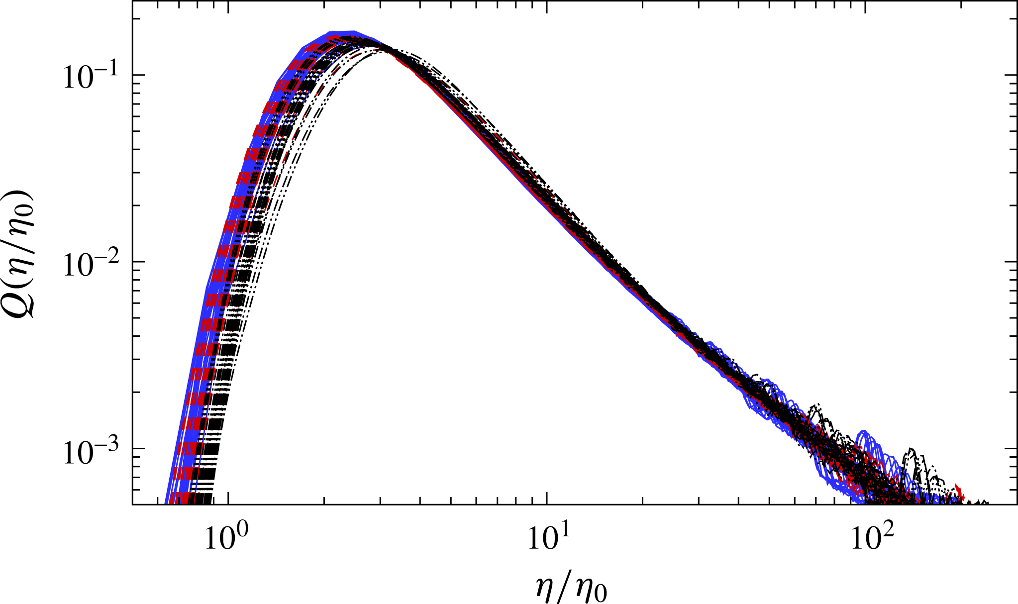
The PDFs calculated from all measurement locations are shown in figure 6 normalized by ${\it\eta}_{0}=LRe_{L}^{-0.73}$ . The distributions normalized this way are consistent with previously reported distributions determined experimentally, numerically and analytically. These distributions are highly skewed and characterized by a broad tail stretching into the large scales, a peak near $2{\it\eta}_{0}$ and a much narrower tail at small scales. Also, close inspection of figure 6 shows that the PDFs do not collapse. As also observed in Hamlington et al. (Reference Hamlington, Krasnov, Boeck and Schumacher2012), there is increasing probability of ${\it\eta}/{\it\eta}_{0}$ occurring at larger scales as $y^{+}\rightarrow 0$ . 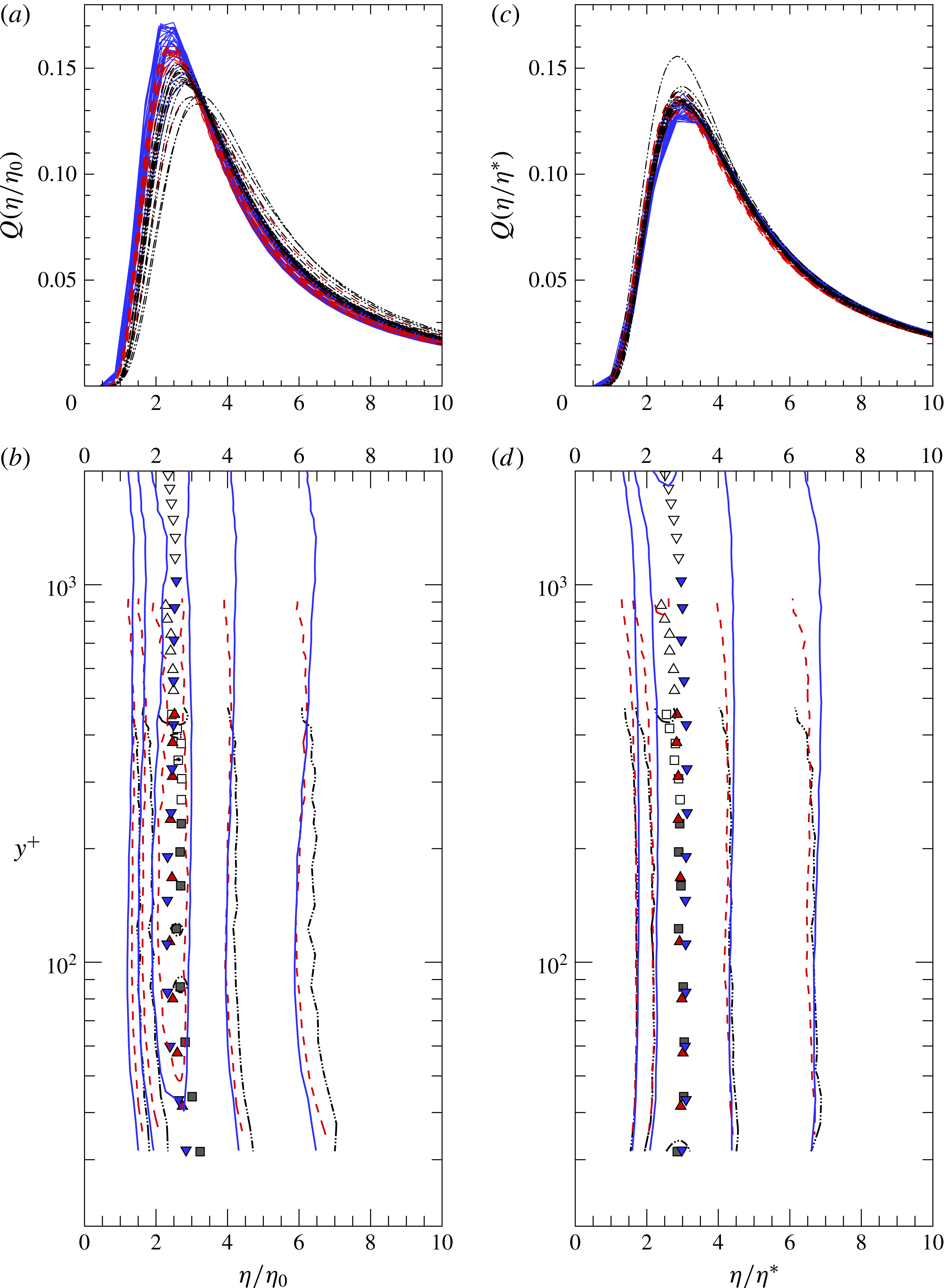This wall-normal dependence is highlighted in figure 7(a,b) which better displays the bias towards large scales for $y^{+}<100$ , highlighted by the trend in the most probable scale, ${\it\eta}_{max}/{\it\eta}_{0}$ . However, unlike Hamlington et al. (Reference Hamlington, Krasnov, Boeck and Schumacher2012), whose investigation was limited to $Re_{{\it\tau}}<600$ , in the present case there is also a slight $Re_{{\it\tau}}$ dependence evident.

Thus, when ${\it\eta}_{0}$ is used as a scaling parameter, as in figure 7(a,b), the results suggest non-universality of the small scales and dependence on the large-scale shear (as also suggested by Morshed et al. (Reference Morshed, Venayagamoorthy and Dasi2013)). Although this non-universality could be attributed to insufficient scale separation at the Reynolds numbers in the present investigation, in the previous sections, $L$ was demonstrated to be an imperfect descriptor for the large scales and hence the normalization parameter ${\it\eta}_{0}$ derived from $L$ is also likely to be an imperfect descriptor of the small scales. Instead, following §§ 3 and 4 we define

Figure 7.

(a) PDFs of local dissipation scales normalized by ${\it\eta}_{0}$ for $y<0.5h$ from $Re_{{\it\tau}}=490$ , 950 and 2080 and (b) isocontours of all PDFs from $Re_{{\it\tau}}=490$ , 950 and 2080 normalized by ${\it\eta}_{0}$ showing wall normal dependence. (c) PDFs of local dissipation scales normalized by ${\it\eta}^{\ast }$ for $y<0.5h$ from $Re_{{\it\tau}}=490$ , 950 and 2080 and (b) isocontours of all PDFs from $Re_{{\it\tau}}=490$ , 950 and 2080 normalized by ${\it\eta}^{\ast }$ showing wall normal dependence. Lines indicate $Re_{{\it\tau}}$ with dash-dot-dot lines indicating $Re_{{\it\tau}}=490$ , dashed lines indicating $Re_{{\it\tau}}=950$ , and solid lines indicating $Re_{{\it\tau}}=2080$ . Symbols in (b,d) as in table 1 showing location of maximum probability with filled symbols indicating measurement points where $y<0.5h$ . Contour levels in (b,d) are spaced 0.025 apart.

The PDFs of ${\it\eta}$ are shown normalized by ${\it\eta}^{\ast }$ in figure 7(c) for $y/h<0.5$ and demonstrate greatly improved collapse when compared to figure 7(a). Although not evident in figure 7(c), some scatter is evident in the small-scale tail of the PDFs normalized by ${\it\eta}^{\ast }$ when viewed on logarithmic axes, but it is likely that this scatter is due to experimental error introduced by the stricter temporal resolution requirements which occur as $Re_{{\it\tau}}$ increases. Note that the analytical PDF of Biferale (Reference Biferale2008) demonstrated Reynolds number dependence in the small-scale tail, although in the form of an increasingly wider tail at higher Reynolds numbers which was the opposite of the behaviour observed in the present results.

The improved collapse when normalized by ${\it\eta}^{\ast }$ is highlighted in the wall-normal dependence presented in figure 7(d). For $y/h<0.5$ , ${\it\eta}_{max}/{\it\eta}^{\ast }$ is constant for all $Re_{{\it\tau}}$ with the contours of $Q({\it\eta}/{\it\eta}^{\ast })$ also showing much less $Re_{{\it\tau}}$ dependence when compared to figure 7(b). For $y/h>0.5$ there is increased Reynolds number dependence in the PDFs as the attached eddy hypothesis used to define $L^{\ast }$ becomes increasingly invalid. However, as noted by both Bailey et al. (Reference Bailey, Hultmark, Schumacher, Yakhot and Smits2009) and Hamlington et al. (Reference Hamlington, Krasnov, Boeck and Schumacher2012), scaling with ${\it\eta}_{0}$ results in collapse of the PDFs far from the wall, re-iterating the inner/outer scaling analogy observed in § 4 in which near the wall, the PDFs can be expected to normalize on ${\it\eta}^{\ast }=f(L^{\ast })$ and far from the wall the PDFs can be expected to normalize on ${\it\eta}_{0}=f(L)$ .