1. Introduction
Elastic micro-capsules are ubiquitous in nature, appearing in the form of seeds, eggs, cells and similar. The elasticity of the cells plays an important role in their proper biological functioning. As examples, red blood cells (RBC) deform significantly in micro-vessels to ease oxygen transportation; leukocytes squeeze through small gaps into the endothelial cell wall during inflammation (Springer Reference Springer1994), as do tumour cells do in tumour metastasis (Hanahan & Weinberg Reference Hanahan and Weinberg2000). On the other hand, artificial micro-capsules are commonly used in the food and cosmetic industry for a controlled release of ingredients (Barthès-Biesel Reference Barthès-Biesel2011) and synthetic nano-capsules promise a precise and targetted drug delivery. The ability of biological and artificial capsules to dynamically adapt, change their shapes and withstand stresses from the surrounding medium has thus attracted much attention from research groups in different fields.
In micro-fluidic applications, one of the most fundamental issues is the behaviour of these tiny deformable structures when interacting with an external applied flow. Early experimental studies discovered several interesting features of RBCs: the well-known tank-treading and tumbling motion in shear flow (Goldsmith & Marlow Reference Goldsmith and Marlow1972; Fischer & Schmid-Schönbein Reference Fischer and Schmid-Schönbein1978), ‘parachute’ shaped deformation (Skalak & Branemark Reference Skalak and Branemark1969) and the ‘zipper’ flow pattern (Gaehtgens, Dührssen & Albrecht Reference Gaehtgens, Dührssen and Albrecht1980) in the micro-capillaries. These observations show that the capsule shape is not given a priori but determined by the dynamic balance of interfacial forces with fluid stresses. Several analytical studies deal with unbounded domains to model tank-treading and tumbling motions of an initially spherical capsule by asymptotic analysis (Barthès-Biesel Reference Barthès-Biesel1980, Reference Barthès-Biesel1981), prove the existence of ‘slipper’ shaped cells in capillary flows (Secomb & Skalak Reference Secomb and Skalak1982), predict the vacillating-breathing behaviour of a vesicle (Misbah Reference Misbah2006) and the swinging–tumbling transition of a capsule (Vlahovska et al. Reference Vlahovska, Young, Danker and Misbah2011).
Numerical simulations have been successfully used to solve the associated nonlinear fluid–structure problem; examples are the deformation of spherical (Pozrikidis Reference Pozrikidis1995, Reference Pozrikidis2001; Foessel et al. Reference Foessel, Walter, Salsac and Barthès-Biesel2011), elliptical (Ramanujan & Pozrikidis Reference Ramanujan and Pozrikidis1998; Walter, Salsac & Barthès-Biesel Reference Walter, Salsac and Barthès-Biesel2011) or RBC-shaped (Pozrikidis Reference Pozrikidis2003) capsules in an unbounded shear flow. However, in a realistic situation, biological cells and artificial capsules are convected in bounded channels or ducts. Motivated by early experiments showing the migration of RBCs towards the pipe centre (Goldsmith Reference Goldsmith1971), Zarda, Chien & Skalak (Reference Zarda, Chien, Skalak, Belytschko and Geers1977) and Özkaya (Reference Özkaya1986) simulated the axisymmetric cellular flow in a cylindrical tube using the finite element method (FEM). Simulations based on the boundary integral method (BIM), combined with FEM for the membrane dynamics, were performed to study capsules tightly squeezed in tubes and square ducts (e.g. Hu, Salsac & Barthès-Biesel Reference Hu, Salsac and Barthès-Biesel2011). Simulations have also addressed complex phenomena like the migration and slipper-shaped deformation of cells (Pozrikidis Reference Pozrikidis2005b ), suspensions of RBCs in a capillary tube (Lei et al. Reference Lei, Fedosov, Caswell and Karniadakis2013), and the shape transition between non-axisymmetric and axisymmetric RBCs (Danker, Vlahovska & Misbah Reference Danker, Vlahovska and Misbah2009; Kaoui, Biros & Misbah Reference Kaoui, Biros and Misbah2009). Inertial effects on the cell migration have also been investigated numerically (Doddi & Bagchi Reference Doddi and Bagchi2008; Shi, Pan & Glowinski Reference Shi, Pan and Glowinski2012).
These previous computational studies focus on the capsule motion in straight geometries. However, capsules are seldom transported in such simple configurations, but rather in highly complicated capillary networks as in the in vivo micro-recirculation for RBCs or through micro-fluidic devices, where corrugations, bifurcations and corners are common. Less is known about the dynamics of capsules in these complex geometries, although these are attracting growing interest thanks to potential biomedical applications. Experiments (Braunmüller, Schmid & Franke Reference Braunmüller, Schmid and Franke2011) and simulations (Noguchi et al. Reference Noguchi, Gompper, Schmid, Wixforth and Franke2010) have shown rich behaviours of RBCs and vesicles going through sawtooth-shaped channels; a transition from shape oscillations to orientational oscillations was identified for such deformable micro-objects, depending on the flow rate and confinement. Two-dimensional FEM computations have been carried out by Barber et al. (Reference Barber, Alberding, Restrepo and Secomb2008) to examine the cell partitioning in small vessel bifurcations, showing that the cells preferentially enter the branch with higher flow rate; such an effect is intensified by the cell migration towards the centre and hindered by obstructions near the bifurcations. Woolfenden & Blyth (Reference Woolfenden and Blyth2011) report two-dimensional simulations of a capsule in a pressure-driven channel with a side branch. These authors found that the capsule deformation strongly depends on the branch angle and the cells selected different paths at the branch junction according to their deformability. Recently, Park & Dimitrakopoulos (Reference Park and Dimitrakopoulos2013) used the spectral boundary element method to investigate the deformation of capsules and droplets passing through a sharp constriction in a square duct. These authors examine the effect of the viscosity ratio on the non-tank-treading capsule dynamics and investigate the flow circulation inside the capsule.
The flow passing around a corner is one of the most basic flow configurations; despite its universality in biological systems and micro-fluidic devices, its influence on deformable micro-objects is not fully understood. Steps in this direction have been taken only recently: the experiments by Rusconi et al. (Reference Rusconi, Lecuyer, Guglielmini and Stone2010) have revealed the rapid formation of bacterial streamers near the corners of a curved micro-channel at low Reynolds number due to the local vortical flow structure. This secondary flow appears as long as the curvature of the boundary varies, even in the inertialess Stokes flow (Lauga, Stroock & Stone Reference Lauga, Stroock and Stone2004). Simulations of an elastic filament in a two-dimensional corner flow (Autrusson et al. Reference Autrusson, Guglielmini, Lecuyer, Rusconi and Stone2011) show that the filament crosses over the curved streamlines in the corner, instead of aligning with the flow as in a rectilinear flow. One of the motivations of this work is to assess whether the corner flow can be used to infer the material properties of soft particles as done by Lefebvre et al. (Reference Lefebvre, Leclerc, Barthès-Biesel, Walter and Edwards-Lévy2008), Chu et al. (Reference Chu, Salsac, Leclerc, Barthès-Biesel, Wurtz and Edwards-Lévy2011) and Hu et al. (Reference Hu, Sévénié, Salsac, Leclerc and Barthès-Biesel2013). In those investigations, the equilibrium shape of capsules moving at a constant speed in confined channels or tubes is compared with that obtained from simulations or theory. As the corner flow is characterized by spatial non-uniformity, the capsule dynamics will undergo a transient evolution that may therefore provide additional information on the membrane properties such as viscoelasticity. Knowledge of the capsule behaviour in spatially developing flows may therefore help to explore the material properties of soft capsules.
In this work, we numerically study the motion and deformation of an individual capsule transported in a duct with a straight and/or a curved corner. A three-dimensional code is developed to compute the motion of deformable capsules in arbitrary configurations. This is based on a boundary integral formulation with Ewald acceleration as suggested by Hernández-Ortiz, de Pablo & Graham (Reference Hernández-Ortiz, de Pablo and Graham2007); the method shares the elegance of both boundary integral and mesh-based methods. Boundary integrals are computed to accurately account for the singular and fast-varying interactions while the smooth part of the solution is handled by a highly parallel general Stokes solver based on the spectral element method. The integration on the membrane is based on a global spectral surface interpolation using spherical harmonics (Zhao et al. Reference Zhao, Isfahani, Olson and Freund2010). Our hybrid scheme couples, therefore, the high accuracy of boundary integrals for the short-ranged interactions to the geometrical flexibility of mesh-based methods (Freund Reference Freund2014). Spherical harmonics are utilized to resolve the membrane dynamics with spectral accuracy. The same implementation has been used to simulate cell sorting by deformability in a micro-fluidic device of complex geometry, i.e. a semi-cylindrical pillar embedded in a divergent channel (Zhu et al. Reference Zhu, Rorai, Dhrubaditya and Brandt2014).
The paper is organized as follows. The geometrical setup and the numerical method are described in § 2. The results are presented in § 3 and their discussion and a summary of the main conclusions is provided in § 4.
2. Problem setup and numerical method
2.1. Flow geometry and numerical procedure
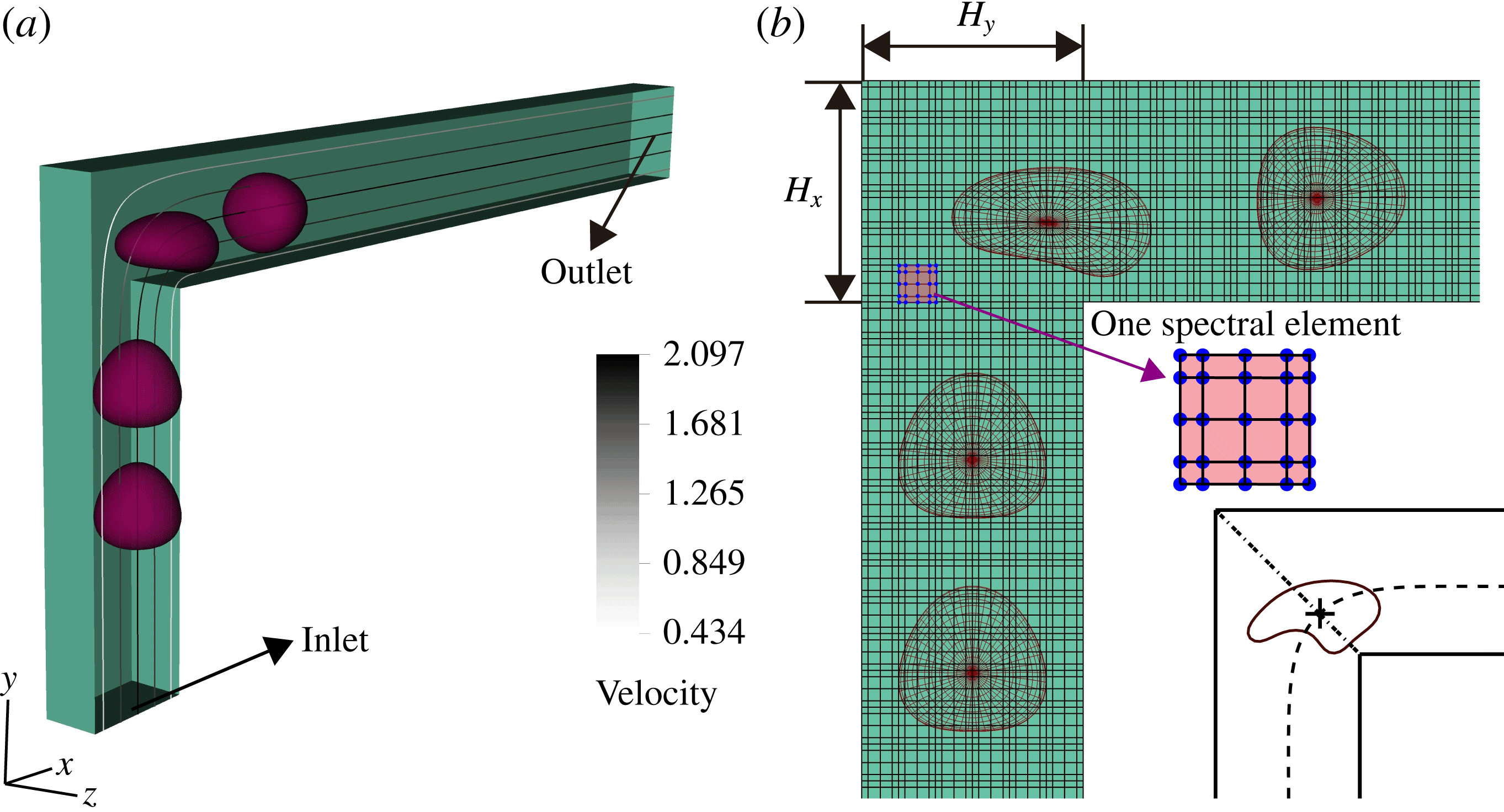
Figure 1 displays the flow configuration and the coordinate system used in the present investigation, where half of the flow domain is removed to better visualize the deforming capsule. We investigate the motion of an elastic capsule transported through a square duct of width
 $H=H_{x}=H_{y}$
; we keep
 $H_{x}=H_{y}$
in this work. In the figure, the streaklines and grey-scale contours, coded by the velocity magnitude, are shown on the
 $x{-}y$
(
 $z=0$
, omitted hereinafter) mid-plane. The duct is characterized by a 90° straight corner.
Flow configuration. (a) A deformable capsule travelling in a square duct with a 90° straight corner, with half of the domain displayed. The analytical velocity profile is imposed at the inlet with a maximum centreline velocity of 2.097. The flow field without capsules is depicted by the streaklines and the grey-scale colour indicates the velocity magnitude. (b) The discretized fluid domain and the capsule at four positions on the
 $x{-}y$
mid-plane. The box with dots represents one spectral element with 5 × 5 × 5 GLL points. In the inset at bottom right, the dashed line denotes the trajectory of the capsule, the dot–dashed line the axis of geometrical symmetry and the cross the capsule centre when located on the axis at instant
 $t=0$
.

We consider an initially spherical capsule of radius
 $a$
, enclosed by an infinitely thin hyperelastic membrane with surface shear modulus
 $G_{s}$
. The fluid inside and outside the capsule has the same density
 ${\it\rho}_{F}$
and viscosity
 ${\it\mu}$
; buoyancy forces and sedimentation effects are neglected.
As capsules are usually small, the Reynolds number
 $\mathit{Re}$
defined with the capsule radius
 $a$
and the characteristic flow velocity
 $V_{C}$
,
 $\mathit{Re}={\it\rho}_{F}V_{C}a/{\it\mu}\ll 1$
. Viscous forces are therefore dominant over inertial forces, and the flow inside and outside the capsule is governed by the linear Stokes equations and determined instantaneously by the boundary conditions. A proper tool to solve the problem is therefore the BIM and we adopt here an accelerated variant of it.
The fluid–structure interaction problem is solved as follows: the flow convects and distorts the capsule while the restoring elastic forces alter the fluid motion (Walter et al. Reference Walter, Salsac, Barthès-Biesel and Tallec2010). We start with an undeformed capsule near the inflow and compute, at each time step, the elastic force on the membrane from the deformed (and out-of-equilibrium) shape of the capsule. Neglecting inertia and Brownian fluctuations, the force density exerted by the capsule onto the fluid is equal to the membrane load. Given this forcing, the velocities of the membrane nodes are computed explicitly with the BIM (see the following section).
2.2. Numerical method
2.2.1. Accelerated BIM
We develop a boundary integral implementation accelerated by the general-geometry Ewald-like method (GGEM), proposed by Hernández-Ortiz et al. (Reference Hernández-Ortiz, de Pablo and Graham2007) and later used in a variety of micro-multiphase simulations (Pranay et al.
Reference Pranay, Anekal, Hernandez-Ortiz and Graham2010; Kumar & Graham Reference Kumar and Graham2011). An introduction is given here; readers are referred to the above-mentioned articles for more details. The surface of the capsule
 $S$
is discretized by
 $M$
points, the Lagrangian mesh points. The elastic force per unit area on the membrane out of equilibrium is denoted
 $\boldsymbol{f}^{e}$
. The force per unit area from the fluid to the membrane is
 $\boldsymbol{f}^{f}$
, with
 $\boldsymbol{f}^{f}+\boldsymbol{f}^{e}=0$
due to the stress continuity. In return, the force per unit volume exerted by the deforming surface onto the fluid at position
 $\boldsymbol{x}$
is
 ${\bf\rho}(\boldsymbol{x})=\int _{S}-\boldsymbol{f}^{f}{\it\delta}(\boldsymbol{x}-\boldsymbol{x}_{m})\text{d}S(\boldsymbol{x}_{m})=\int _{S}\boldsymbol{f}^{e}{\it\delta}(\boldsymbol{x}-\boldsymbol{x}_{m})\text{d}S(\boldsymbol{x}_{m})$
, with
 ${\it\delta}$
the Dirac delta function and
 $\boldsymbol{x}_{m}$
the integration variable, indicating that the integration is performed on the membrane surface. We thus need to solve the following equations for the fluid in the inertialess Stokes regime:
 $$\begin{eqnarray}\displaystyle & \displaystyle -\boldsymbol{{\rm\nabla}}p(\boldsymbol{x})+{\it\mu}{\rm\nabla}^{2}\boldsymbol{u}(\boldsymbol{x})+\int _{S}\boldsymbol{f}^{e}(\boldsymbol{x}_{m}){\it\delta}(\boldsymbol{x}-\boldsymbol{x}_{m})\text{d}S(\boldsymbol{x}_{m})=0, & \displaystyle\end{eqnarray}$$
 $$\begin{eqnarray}\displaystyle & \boldsymbol{{\rm\nabla}}\boldsymbol{\cdot }\boldsymbol{u}(\boldsymbol{x})=0, & \displaystyle\end{eqnarray}$$
 $p$
and
 $\boldsymbol{u}$
denote the pressure and fluid velocity and
 ${\it\mu}$
is the fluid dynamic viscosity. Owing to the linearity of the Stokes problem, the flow field can be expressed as a boundary integral on the surface of the capsule only,
 $$\begin{eqnarray}\boldsymbol{u}(\boldsymbol{x})=\boldsymbol{u}^{\infty }(\boldsymbol{x})+\int _{S}\unicode[STIX]{x1D642}(\boldsymbol{x},\boldsymbol{x}_{m})\boldsymbol{\cdot }\boldsymbol{f}^{e}(\boldsymbol{x}_{m})\text{d}S(\boldsymbol{x}_{m}),\end{eqnarray}$$
where
 $\boldsymbol{u}^{\infty }(\boldsymbol{x})$
is the velocity field of the undisturbed flow and
 $\unicode[STIX]{x1D642}(\boldsymbol{x}^{\prime },\boldsymbol{y}^{\prime })$
is the free-space Green’s function of the Stokes problem, also known as the Stokeslet or Oseen–Burgers tensor,
 $$\begin{eqnarray}\unicode[STIX]{x1D642}(\boldsymbol{x}^{\prime },\boldsymbol{y}^{\prime })=\frac{1}{8{\rm\pi}{\it\mu}r}\left({\bf\delta}+\frac{\left(\boldsymbol{x}^{\prime }-\boldsymbol{y}^{\prime }\right)\left(\boldsymbol{x}^{\prime }-\boldsymbol{y}^{\prime }\right)}{r^{2}}\right)\!,\end{eqnarray}$$
with
 $r=|\boldsymbol{x}^{\prime }-\boldsymbol{y}^{\prime }|$
.
The GGEM method decomposes the force per unit volume
 ${\bf\rho}(\boldsymbol{x})$
into a local part
 ${\bf\rho}^{l}(\boldsymbol{x})$
and a global part
 ${\bf\rho}^{g}(\boldsymbol{x})$
, with
 ${\bf\rho}(\boldsymbol{x})={\bf\rho}^{l}(\boldsymbol{x})+{\bf\rho}^{g}(\boldsymbol{x})$
and
 $$\begin{eqnarray}\displaystyle & \displaystyle {\bf\rho}^{l}(\boldsymbol{x})=\int _{S}\boldsymbol{f}^{e}(\boldsymbol{x}_{m})[{\it\delta}-g(\boldsymbol{x}-\boldsymbol{x}_{m})]\text{d}S(\boldsymbol{x}_{m}), & \displaystyle\end{eqnarray}$$
 $$\begin{eqnarray}\displaystyle & \displaystyle {\bf\rho}^{g}(\boldsymbol{x})=\int _{S}\boldsymbol{f}^{e}(\boldsymbol{x}_{m})g(\boldsymbol{x}-\boldsymbol{x}_{m})\text{d}S(\boldsymbol{x}_{m}), & \displaystyle\end{eqnarray}$$
 $g(\boldsymbol{x}^{\prime })$
is a quasi-Gaussian function used to smooth the Dirac delta function,
 $$\begin{eqnarray}g(\boldsymbol{x}^{\prime })=\left({\it\alpha}_{cut}^{3}/{\rm\pi}^{3/2}\right)\text{exp}\left(-{\it\alpha}_{cut}^{2}|\boldsymbol{x}^{\prime }|^{2}\right)\left[5/2-{\it\alpha}_{cut}^{2}|\boldsymbol{x}^{\prime }|^{2}\right],\end{eqnarray}$$
where
 ${\it\alpha}_{cut}^{-1}$
indicates the length scale over which the smoothing is active.
The Stokes problem in (2.1) is therefore decomposed into two problems: one for the flow induced by the local force
 ${\bf\rho}^{l}(\boldsymbol{x})$
, hence called the local problem, and one for its global counterpart
 ${\bf\rho}^{g}(\boldsymbol{x})$
. The velocity field
 $\boldsymbol{u}(\boldsymbol{x})$
is the sum of the local velocity
 $\boldsymbol{u}^{l}(\boldsymbol{x})$
and global velocity
 $\boldsymbol{u}^{g}(\boldsymbol{x})$
,
 $\boldsymbol{u}(\boldsymbol{x})=\boldsymbol{u}^{l}(\boldsymbol{x})+\boldsymbol{u}^{g}(\boldsymbol{x})$
. The local problem accounts for the singular and short-ranged interaction while the global problem accounts for the smooth and long-ranged interactions. These are solved by different numerical methods; the local solution is calculated by the BIM due to its superior accuracy in resolving fast-decaying interactions, while the global problem is handled by a mesh-based solver that provides geometrical flexibility.
The modified Stokeslet pertaining the local problem can be shown to be
 $$\begin{eqnarray}\unicode[STIX]{x1D642}^{l}(\boldsymbol{x}^{\prime })=\frac{1}{8{\rm\pi}{\it\mu}}\left({\bf\delta}+\frac{\boldsymbol{x}^{\prime }\boldsymbol{x}^{\prime }}{|\boldsymbol{x}^{\prime }|^{2}}\right)\frac{\text{erfc}({\it\alpha}_{cut}|\boldsymbol{x}^{\prime }|)}{|\boldsymbol{x}^{\prime }|}-\frac{1}{8{\rm\pi}{\it\mu}}\left({\bf\delta}-\frac{\boldsymbol{x}^{\prime }\boldsymbol{x}^{\prime }}{|\boldsymbol{x}^{\prime }|^{2}}\right)\frac{2{\it\alpha}_{cut}}{{\rm\pi}^{1/2}}\text{exp}(-{\it\alpha}_{cut}^{2}|\boldsymbol{x}^{\prime }|^{2}),\end{eqnarray}$$
so that the velocity field
 $\boldsymbol{u}^{l}(\boldsymbol{x})$
of the local solution can be obtained as
 $$\begin{eqnarray}\boldsymbol{u}^{l}(\boldsymbol{x})=\int _{S}\unicode[STIX]{x1D642}^{l}(\boldsymbol{x},\boldsymbol{x}_{m})\boldsymbol{\cdot }\boldsymbol{f}^{e}(\boldsymbol{x}_{m})\text{d}S(\boldsymbol{x}_{m}).\end{eqnarray}$$
Equation (2.9) can be integrated by classical boundary integral implementations. Regularized Stokeslets can be used to facilitate the calculations, as done in, among others, Hernández-Ortiz et al. (Reference Hernández-Ortiz, de Pablo and Graham2007) and Pranay et al. (Reference Pranay, Anekal, Hernandez-Ortiz and Graham2010). Nonetheless, the BIM with regularization suffers a degradation of the numerical accuracy and robustness for cases involving strong confinement or closely packed objects. Singular and nearly singular integration is necessary to achieve the required accuracy in these cases (Huang & Cruse Reference Huang and Cruse1993; Zhu, Lauga & Brandt Reference Zhu, Lauga and Brandt2013), and this is the approach pursued here.
As the modified Stokeslet
 $\unicode[STIX]{x1D642}^{l}(\boldsymbol{x}^{\prime })$
decays rapidly, the integral of (2.9) is assumed to be zero when the distance between
 $\boldsymbol{x}$
and
 $\boldsymbol{x}_{m}$
is above a cut-off radius
 $R_{cut}$
. We choose
 $R_{cut}=4{\it\alpha}_{cut}^{-1}$
and
 ${\it\alpha}_{cut}=a^{-1}$
as in the work of Pranay et al. (Reference Pranay, Anekal, Hernandez-Ortiz and Graham2010). The alternative value
 $R_{cut}=5{\it\alpha}_{cut}^{-1}$
has also been tested for some of the cases and no significant differences have been observed.
The modified Stokeslet
 $\unicode[STIX]{x1D642}^{l}(\boldsymbol{x}^{\prime })$
is valid for an unbounded domain, thus the local velocity
 $\boldsymbol{u}^{l}(\boldsymbol{x})$
does not account for the influence of any additional boundaries. The global velocity will therefore be defined in such a way that the sum of the two will satisfy the required boundary conditions: no slip at the solid wall
 ${\it\Omega}$
in the cases investigated here,
 $\boldsymbol{u}^{l}(\boldsymbol{x}_{{\it\Omega}})+\boldsymbol{u}^{g}(\boldsymbol{x}_{{\it\Omega}})=0$
. The global problem amounts to solving the Stokes problem in the domain of interest with the known volume forcing
 ${\bf\rho}^{g}(\boldsymbol{x})$
and boundary conditions defined by the solution of the local problem. This allows the use of a variety of efficient and accurate numerical methods for the solution of the Stokes equations in any complex geometry. Here, we compute the global solution with Stokes module of the open-source Navier–Stokes solver NEK5000 (Fischer, Lottes & Kerkemeier Reference Fischer, Lottes and Kerkemeier2008b
), using the spectral element method. NEK5000 has been extensively used for stability analysis (Schrader et al.
Reference Schrader, Brandt, Mavriplis and Henningson2010) and turbulent flows (Fischer et al.
Reference Fischer, Lottes, Pointer and Siegel2008a
) in complex domains. Akin to the FEM, the physical domain is decomposed into elements, with each element subdivided into arrays of Gauss–Lobatto–Legendre (GLL) nodes for the velocity and Gauss–Legendre (GL) nodes for the pressure field. The Galerkin approximation is employed for the spatial discretization with different velocity and pressure spaces, the so-called
 $\mathbb{P}_{N}-\mathbb{P}_{N-2}$
approach (Maday & Patera Reference Maday and Patera1989). Accordingly, the velocity (respectively pressure) space consists of
 $N$
th- (respectively
 $(N-2)$
th-) order Lagrange polynomial interpolants, defined on the GLL (respectively GL) quadrature points in each element. Note that we do not solve the Navier–Stokes equations with a very small but finite Reynolds number, but instead use the steady Stokes solver of NEK5000 at each time step. NEK5000 is chosen here for its spectral accuracy, high parallel performance and most importantly its geometric flexibility, fully exploiting the general-geometry merit of GGEM.
The global problem is solved only on the Eulerian mesh points, which do not necessarily coincide with the Lagrangian mesh points on the membrane (see figure 1). Thus, at each time step, an interpolation from the global solution is performed to obtain the global velocity
 $\boldsymbol{u}^{g}(\boldsymbol{x}_{i}),~i=1,2,3,\dots ,M,$
of the Lagrangian points. The interpolation error is minimized thanks to the spectral accuracy of NEK5000. The velocities of the Lagrangian points are obtained by summing up the local and global velocities. We use a third-order Adam–Bashforth time-integration scheme to update the position of those points.
2.2.2. Spectral method for the membrane dynamics
The membrane loading was calculated as linear piece-wise functions on triangular meshes by Pozrikidis (Reference Pozrikidis1995), Ramanujan & Pozrikidis (Reference Ramanujan and Pozrikidis1998) and Li & Sarkar (Reference Li and Sarkar2008) among others. FEM has also been implemented by Walter et al. (Reference Walter, Salsac, Barthès-Biesel and Tallec2010) for its generality and versatility. Bi-cubic B-splines interpolation functions were adopted by Lac, Morel & Barthès-Biesel (Reference Lac, Morel and Barthès-Biesel2007) to obtain accurate results at a reasonably high computational cost. Alternatively, an accurate spectral boundary element algorithm was used by Dodson & Dimitrakopoulos (Reference Dodson and Dimitrakopoulos2009), Kuriakose & Dimitrakopoulos (Reference Kuriakose and Dimitrakopoulos2011, Reference Kuriakose and Dimitrakopoulos2013), thus coupling the numerical accuracy of the spectral method and the geometric flexibility of the boundary element method. Another attractive alternative is the global spectral method. Fourier spectral interpolation and spherical harmonics have been used for two-dimensional (Freund Reference Freund2007) and three-dimensional simulations (Kessler, Finken & Seifert Reference Kessler, Finken and Seifert2008; Zhao et al. Reference Zhao, Isfahani, Olson and Freund2010). Here, we follow the approach of Zhao et al. (Reference Zhao, Isfahani, Olson and Freund2010), briefly outlined below.
We map the capsule surface onto the surface of the unit reference sphere
 $\mathbb{S}^{2}$
, using its spherical angles
 $({\it\theta},{\it\phi})$
for the parametrization. The parameter space
 $\{({\it\theta},{\it\phi})|0\leqslant {\it\theta}\leqslant {\rm\pi},0\leqslant {\it\phi}\leqslant 2{\rm\pi}\}$
is discretized by a quadrilateral grid consisting of GL quadrature points in
 ${\it\theta}$
and uniform intervals in
 ${\it\phi}$
. All other surface quantities are defined on the same mesh. The surface coordinates
 $\boldsymbol{x}({\it\theta},{\it\phi})$
are expressed by a truncated series of spherical harmonic functions,
 $$\begin{eqnarray}\boldsymbol{x}({\it\theta},{\it\phi})=\mathop{\sum }_{n=0}^{N_{SH}}\mathop{\sum }_{m=0}^{n}\bar{P}_{n}^{m}(\cos {\it\theta})(\boldsymbol{a}_{nm}\cos m{\it\phi}+\boldsymbol{b}_{nm}\sin m{\it\phi}),\end{eqnarray}$$
yielding
 $N_{SH}^{2}$
spherical harmonic modes. The corresponding normalized Legendre polynomials are
 $$\begin{eqnarray}\bar{P}_{n}^{m}(x)=\frac{1}{2^{n}n!}\sqrt{\frac{\left(2n+1\right)\left(n-m\right)!}{2(n+m)!}}\left(1-x^{2}\right)^{m/2}\frac{\text{d}^{n+m}}{\text{d}x^{n+m}}\left(x^{2}-1\right)^{n}.\end{eqnarray}$$
Both forward and backward transformations are calculated with the SPHEREPACK library (Adams & Swarztrauber Reference Adams and Swarztrauber1997; Swarztrauber & Spotz Reference Swarztrauber and Spotz2000). Aliasing errors arise due to the nonlinearities induced by the membrane model and the complicated geometry (products, roots and inverse operations needed to calculate the geometric quantities introduced below). We implement an approximate dealiasing by performing the nonlinear operations on
 $M_{SH}>N_{SH}$
points and filtering the result back to
 $N_{SH}$
points. A detailed discussion on this issue is provided in Freund & Zhao (Reference Freund, Zhao and Pozrikidis2010).
A point on the surface is expressed by the curvilinear coordinates,
 $({\it\xi}^{1},{\it\xi}^{2})=({\it\theta},{\it\phi})$
, defined on the covariant base,
 $(\boldsymbol{a}_{1},\boldsymbol{a}_{2},\boldsymbol{a}_{3})$
, following the local deformation. The base vectors are
 $$\begin{eqnarray}\boldsymbol{a}_{1}=\frac{\partial \boldsymbol{x}}{\partial {\it\theta}},\quad \boldsymbol{a}_{2}=\frac{\partial \boldsymbol{x}}{\partial {\it\phi}},\quad \boldsymbol{a}_{3}=\boldsymbol{n}=\frac{\boldsymbol{a}_{1}\times \boldsymbol{a}_{2}}{|\boldsymbol{a}_{1}\times \boldsymbol{a}_{2}|},\end{eqnarray}$$
and the covariant and contravariant metric tensors
 $$\begin{eqnarray}\unicode[STIX]{x1D622}_{{\it\alpha}{\it\beta}}=\boldsymbol{a}_{{\it\alpha}}\boldsymbol{\cdot }\boldsymbol{a}_{{\it\beta}},\quad \unicode[STIX]{x1D622}^{{\it\alpha}{\it\beta}}=\boldsymbol{a}^{{\it\alpha}}\boldsymbol{\cdot }\boldsymbol{a}^{{\it\beta}},\end{eqnarray}$$
where
 ${\it\alpha},{\it\beta}=1,2$
. The base vectors and metric tensors are also defined for the undeformed state and denoted here by capital letters (
 $\boldsymbol{A}^{{\it\alpha}}$
,
 $\unicode[STIX]{x1D608}^{{\it\alpha}{\it\beta}}$
).
The second fundamental form coefficient of the surface is
 $\unicode[STIX]{x1D623}_{{\it\alpha}{\it\beta}}=\boldsymbol{n}\boldsymbol{\cdot }(\partial \boldsymbol{a}_{{\it\alpha}}/\partial {\it\xi}^{{\it\beta}})$
and the two invariants of the transformation
 $I_{1}$
and
 $I_{2}$
are defined as
 $$\begin{eqnarray}I_{1}=\unicode[STIX]{x1D608}^{{\it\alpha}{\it\beta}}\unicode[STIX]{x1D622}_{{\it\alpha}{\it\beta}}-2,\quad I_{2}=|\unicode[STIX]{x1D608}^{{\it\alpha}{\it\beta}}|\,|\unicode[STIX]{x1D622}_{{\it\alpha}{\it\beta}}|-1.\end{eqnarray}$$
 $I_{1}$
and
 $I_{2}$
can also be determined from the principal dilations
 ${\it\lambda}_{1}$
and
 ${\it\lambda}_{2}$
,
 $$\begin{eqnarray}I_{1}={\it\lambda}_{1}^{2}+{\it\lambda}_{2}^{2}-2,\quad I_{2}={\it\lambda}_{1}^{2}{\it\lambda}_{2}^{2}-1=J_{2}^{2}-1.\end{eqnarray}$$
The Jacobian,
 $J_{s}={\it\lambda}_{1}{\it\lambda}_{2}$
, shows the ratio of the deformed to the undeformed surface area. We compute the in-plane Cauchy stress tensor
 $\unicode[STIX]{x1D64F}$
, from the strain energy function per unit area of the undeformed membrane,
 $W_{S}(I_{1},I_{2})$
,
 $$\begin{eqnarray}\unicode[STIX]{x1D64F}=\frac{1}{J_{s}}\unicode[STIX]{x1D641}\boldsymbol{\cdot }\frac{\partial W_{S}}{\partial \unicode[STIX]{x1D65A}}\boldsymbol{\cdot }\unicode[STIX]{x1D641}^{\text{T}},\end{eqnarray}$$
where
 $\unicode[STIX]{x1D641}$
is
 $\boldsymbol{a}_{{\it\alpha}}\otimes \boldsymbol{A}^{{\it\alpha}}$
and
 $\unicode[STIX]{x1D65A}=(\unicode[STIX]{x1D641}^{\text{T}}\boldsymbol{\cdot }\unicode[STIX]{x1D641}-\unicode[STIX]{x1D644})/2$
is the Green–Lagrange stain tensor. Equation (2.16) can be further expressed by components as
 $$\begin{eqnarray}\unicode[STIX]{x1D61B}^{{\it\alpha}{\it\beta}}=\frac{2}{J_{s}}\frac{\partial W_{S}}{\partial I_{1}}\unicode[STIX]{x1D608}^{{\it\alpha}{\it\beta}}+2J_{s}\frac{\partial W_{S}}{\partial I_{2}}\unicode[STIX]{x1D622}^{{\it\alpha}{\it\beta}}.\end{eqnarray}$$
We employ a widely used model of the strain energy function
 $W_{S}$
in our study, the neo-Hookean law (NH) (Green & Adkins Reference Green and Adkins1970) formulated as
 $$\begin{eqnarray}W_{S}^{NH}=\frac{G_{s}}{2}\left(I_{1}-1+\frac{1}{I_{2}+1}\right)\!,\end{eqnarray}$$
where
 $G_{s}$
is the surface shear modulus. The local equilibrium connects
 $\unicode[STIX]{x1D64F}$
with the external membrane load
 $\boldsymbol{q}$
, as
 $$\begin{eqnarray}\boldsymbol{{\rm\nabla}}_{s}\boldsymbol{\cdot }\unicode[STIX]{x1D64F}+\boldsymbol{q}=0,\end{eqnarray}$$
where (
 $\boldsymbol{{\rm\nabla}}_{s}\boldsymbol{\cdot }$
) is the surface divergence operator in the deformed state. In curvilinear coordinates, the load vector is written as
 $\boldsymbol{q}=q^{{\it\beta}}\boldsymbol{a}_{{\it\beta}}+q^{n}\boldsymbol{n},\;{\it\beta}=1,2$
. The local balance in (2.19) is further decomposed into tangential and normal components,
 $$\begin{eqnarray}\displaystyle & \displaystyle \frac{\partial \!\unicode[STIX]{x1D61B}^{{\it\alpha}{\it\beta}}}{\partial {\it\xi}^{{\it\alpha}}}+{\it\Gamma}_{{\it\alpha}{\it\lambda}}^{{\it\alpha}}\unicode[STIX]{x1D61B}^{{\it\lambda}{\it\beta}}+{\it\Gamma}_{{\it\alpha}{\it\lambda}}^{{\it\beta}}\unicode[STIX]{x1D61B}^{{\it\alpha}{\it\lambda}}+q^{{\it\beta}}=0,\quad {\it\beta}=1,2, & \displaystyle\end{eqnarray}$$
 $$\begin{eqnarray}\displaystyle & \unicode[STIX]{x1D61B}^{{\it\alpha}{\it\beta}}\unicode[STIX]{x1D623}_{{\it\alpha}{\it\beta}}+q^{n}=0, & \displaystyle\end{eqnarray}$$
 ${\it\Gamma}_{{\it\alpha}{\it\lambda}}^{{\it\beta}}$
are the Christoffel symbols.
We incorporate bending stiffness into our model using the linear isotropic model for the bending moment
 $\boldsymbol{M}$
:
 $\unicode[STIX]{x1D614}_{{\it\beta}}^{{\it\alpha}}=-G_{\mathit{B}}(\unicode[STIX]{x1D623}_{{\it\beta}}^{{\it\alpha}}-\unicode[STIX]{x1D609}_{{\it\beta}}^{{\it\alpha}})$
, where
 $G_{\mathit{B}}$
is the bending modulus, and
 $\unicode[STIX]{x1D623}_{{\it\beta}}^{{\it\alpha}}$
is the mixed version of the second fundamental form coefficients (
 $\unicode[STIX]{x1D609}_{{\it\beta}}^{{\it\alpha}}$
corresponds to that of the reference configuration). Considering the local torque balance with bending moments exerted on the membrane, we obtain the transverse shear vector
 $\boldsymbol{Q}$
and in-plane stress tensor
 $\unicode[STIX]{x1D64F}$
,
 $$\begin{eqnarray}\displaystyle & \unicode[STIX]{x1D614}_{|{\it\alpha}}^{{\it\alpha}{\it\beta}}-Q^{{\it\beta}}=0, & \displaystyle\end{eqnarray}$$
 $$\begin{eqnarray}\displaystyle & {\bf\varepsilon}_{{\it\alpha}{\it\beta}}(\unicode[STIX]{x1D61B}^{{\it\alpha}{\it\beta}}-\unicode[STIX]{x1D623}_{{\it\gamma}}^{{\it\alpha}}\unicode[STIX]{x1D614}^{{\it\gamma}{\it\beta}})=0, & \displaystyle\end{eqnarray}$$
 $\text{}_{|{\it\alpha}}$
’ denotes the covariant derivative and
 ${\bf\varepsilon}$
the two-dimensional Levi-Civita tensor. Equation (2.23) determines the antisymmetric part of the in-plane stress tensor, which is always zero as proved in Zhao et al. (Reference Zhao, Isfahani, Olson and Freund2010). Including the transverse shear stress
 $\boldsymbol{Q}$
, the local equilibrium of the stress, including bending, gives
 $$\begin{eqnarray}\displaystyle & \displaystyle \frac{\partial \unicode[STIX]{x1D61B}^{{\it\alpha}{\it\beta}}}{\partial {\it\xi}^{{\it\alpha}}}+{\it\Gamma}_{{\it\alpha}{\it\lambda}}^{{\it\alpha}}\unicode[STIX]{x1D61B}^{{\it\lambda}{\it\beta}}+{\it\Gamma}_{{\it\alpha}{\it\lambda}}^{{\it\beta}}\unicode[STIX]{x1D61B}^{{\it\alpha}{\it\lambda}}-\unicode[STIX]{x1D623}_{{\it\alpha}}^{{\it\beta}}Q^{{\it\alpha}}+q^{{\it\beta}}=0,\quad {\it\beta}=1,2, & \displaystyle\end{eqnarray}$$
 $$\begin{eqnarray}\displaystyle & \unicode[STIX]{x1D61B}^{{\it\alpha}{\it\beta}}\unicode[STIX]{x1D623}_{{\it\alpha}{\it\beta}}+Q_{|{\it\alpha}}^{{\it\alpha}}+q^{n}=0. & \displaystyle\end{eqnarray}$$
2.2.3. Singular and nearly singular integration
In this section, we report the scheme for singular and nearly singular integration based on the spectral surface discretization. We mostly follow the approach in Zhao et al. (Reference Zhao, Isfahani, Olson and Freund2010), which is briefly described here for the sake of completeness. We rewrite the boundary integral equation (2.9) in its general form as
 $$\begin{eqnarray}\mathscr{I}(\boldsymbol{x}_{0})=\int _{S}K(\boldsymbol{x},\boldsymbol{x}_{0})g(\boldsymbol{x})\text{d}S(\boldsymbol{x})=\int _{\mathbb{S}^{2}}K(\boldsymbol{x}({\it\theta},{\it\phi}),\boldsymbol{x}_{0})g\left(\boldsymbol{x}({\it\theta},{\it\phi})\right)J({\it\theta},{\it\phi})\text{d}{\it\theta}\text{d}{\it\phi},\end{eqnarray}$$
where
 $K$
is one component of the Green’s function kernel, the modified Stokeslet in (2.8) in our case,
 $g$
is a smooth function defined in
 $S$
and
 $J=|(\partial \boldsymbol{x}/\partial {\it\theta})\times (\partial \boldsymbol{x}/\partial {\it\phi})|$
the Jacobian. If the point
 $\boldsymbol{x}_{0}$
is sufficiently far from the membrane surface
 $S$
,
 $K$
is smooth and the integral
 $\mathscr{I}(\boldsymbol{x}_{0})$
can be computed as
 $$\begin{eqnarray}\mathscr{I}(\boldsymbol{x}_{0})=\mathop{\sum }_{k=1}^{M=N_{SH}\times 2N_{SH}}K(\boldsymbol{x}_{k},\boldsymbol{x}_{0})g(\boldsymbol{x}_{k})J({\it\theta}_{k},{\it\phi}_{k}){\it\omega}_{k},\end{eqnarray}$$
where
 ${\it\omega}_{k}$
is the weight of the
 $k$
th discretized point. If
 $\boldsymbol{x}_{0}$
lies on the boundary
 $S$
, the kernel function
 $K(\boldsymbol{x},\boldsymbol{x}_{0})$
becomes singular: in this case, a naive integration using (2.27) would give low accuracy; this so-called singular integration needs a special treatment. As
 $\boldsymbol{x}_{0}$
is very close to
 $S$
,
 $K(\boldsymbol{x},\boldsymbol{x}_{0})$
becomes nearly singular, also requiring additional care. We adopt here the approach denoted as floating partition of unity (Bruno & Kunyansky Reference Bruno and Kunyansky2001). In the singular case,
 $\boldsymbol{x}_{0}$
on the surface, we define
 $s(\boldsymbol{x},\boldsymbol{x}_{0})$
as the contour length along the great circle connecting
 $\boldsymbol{x}$
and
 $\boldsymbol{x}_{0}$
on the reference sphere
 $\mathbb{S}^{2}$
. This is used to define a mask function
 ${\it\eta}(s(\boldsymbol{x},\boldsymbol{x}_{0}))$
,
 $$\begin{eqnarray}{\it\eta}(s)=\left\{\begin{array}{@{}ll@{}}\displaystyle \exp \!\left(\frac{2\exp (-1/t)}{t-1}\right)\quad & \text{if }t=s/s_{cut}<1,\\ 0\quad & \text{if }s\geqslant s_{cut},\end{array}\right.\end{eqnarray}$$
where
 $s_{cut}$
is a cut-off radius. With the mask function
 ${\it\eta}(s)$
, the boundary integral
 $\mathscr{I}(\boldsymbol{x}_{0})$
is decomposed into two parts, a singular part
 $\mathscr{I}_{singular}(\boldsymbol{x}_{0})$
and a smooth part
 $\mathscr{I}_{smooth}(\boldsymbol{x}_{0})$
:
 $$\begin{eqnarray}\displaystyle & \mathscr{I}(\boldsymbol{x}_{0})=\mathscr{I}_{singular}(\boldsymbol{x}_{0})+\mathscr{I}_{smooth}(\boldsymbol{x}_{0}), & \displaystyle\end{eqnarray}$$
 $$\begin{eqnarray}\displaystyle & \mathscr{I}_{singular}(\boldsymbol{x}_{0})=\displaystyle \int _{S}{\it\eta}(s(\boldsymbol{x},\boldsymbol{x}_{0}))K(\boldsymbol{x},\boldsymbol{x}_{0})g(\boldsymbol{x})\text{d}S(\boldsymbol{x}), & \displaystyle\end{eqnarray}$$
 $$\begin{eqnarray}\displaystyle & \mathscr{I}_{smooth}(\boldsymbol{x}_{0})=\displaystyle \int _{S}\left[1-{\it\eta}(s(\boldsymbol{x},\boldsymbol{x}_{0}))\right]K(\boldsymbol{x},\boldsymbol{x}_{0})g(\boldsymbol{x})\text{d}S(\boldsymbol{x}). & \displaystyle\end{eqnarray}$$
 $\boldsymbol{x}$
and
 $\boldsymbol{x}_{0}$
coincide so that the integral can be computed accurately using (2.27). The singular part has non-zero values only on the spherical patch of radius
 $s_{cut}$
, and it can be integrated using local polar coordinates defined on that patch,
 $$\begin{eqnarray}\mathscr{I}_{singular}(\boldsymbol{x}_{0})=\int _{0}^{2{\rm\pi}}\int _{0}^{s_{cut}}{\it\eta}(s)K(\boldsymbol{x}(s,{\it\psi}),\boldsymbol{x}_{0})g(s,{\it\psi})J^{\prime }(s,{\it\psi})\text{d}s\text{d}{\it\psi},\end{eqnarray}$$
where
 $J^{\prime }(s,{\it\psi})=|(\partial \boldsymbol{x}/\partial s)\times (\partial \boldsymbol{x}/\partial {\it\psi})|$
is the Jacobian of the transformation. We apply Gauss quadrature along the radial direction
 $s\in [0,s_{cut}]$
and sum over the circumferential direction
 ${\it\psi}\in [0,2{\rm\pi}]$
. The radius of the patch is chosen to be
 $s_{cut}={\rm\pi}/\sqrt{N_{SH}}$
(see the detailed discussion in Zhao et al.
Reference Zhao, Isfahani, Olson and Freund2010). Because the quadrature points do not necessarily coincide with the discretization points, interpolation is needed to obtain quantities such as
 $g(s,{\it\psi})$
. Bi-cubic spline interpolation is performed here: firstly, we compute
 $g$
on a uniform mesh in
 ${\it\theta}$
and
 ${\it\phi}$
based on the spherical harmonic coefficients; the mesh is then extended from
 ${\it\theta}\in [0,{\rm\pi}]$
to
 ${\it\theta}\in [0,2{\rm\pi}]$
exploiting the symmetry
 $g(2{\rm\pi}-{\it\theta},{\rm\pi}+{\it\phi})=g({\it\theta},{\it\phi})$
;
 $g$
is periodic in both directions on the extended domain and its derivatives can be accurately computed by Fourier transform; we finally construct the bi-cubic spline approximation using the function derivatives.
For the nearly singular integration, we first find the projection of
 $\boldsymbol{x}_{0}$
onto the membrane surface,
 $\boldsymbol{x}_{0}^{proj}$
, and then compute the boundary integral on the spherical patch centred at
 $\boldsymbol{x}_{0}^{proj}$
. A
 $\sinh$
transformation is applied in the radial direction in order to move the quadrature points closer to
 $\boldsymbol{x}_{0}^{proj}$
(Johnston & Elliott Reference Johnston and Elliott2005), better resolving the fast-varying Green’s function near
 $\boldsymbol{x}_{0}^{proj}$
.
2.3. Non-dimensionalization
The capsule membrane is characterized by its resistance to shearing and bending. The capillary number
 $\mathit{Ca}$
, the ratio of viscous over elastic forces, is defined based on the surface shear modulus
 $G_{s}$
,
 $$\begin{eqnarray}\mathit{Ca}=\frac{{\it\mu}V_{C}}{G_{s}},\end{eqnarray}$$
where we use the mean velocity as the characteristic flow velocity
 $V_{C}$
. The reduced bending modulus,
 $Cb$
, is the ratio of the bending and shearing moduli,
 $Cb=G_{B}/a^{2}G_{s}$
. We use the radius of the capsule
 $a$
as the reference length scale, so that the characteristic time scale is
 $T=a/V_{C}$
.
2.4. Validation
We first introduce the parameters used in the discretization. As mentioned in § 2.2.1,
 ${\it\alpha}_{cut}=a^{-1}=1$
and
 $R_{cut}=4{\it\alpha}_{cut}^{-1}$
are adopted following the recommendation in Pranay et al. (Reference Pranay, Anekal, Hernandez-Ortiz and Graham2010). Cubic spectral elements of size 1 with 5 × 5 × 5 GLL points are used to discretize the fluid domain, where the mean grid spacing
 $h_{mean}=1/4$
well satisfies the relation
 ${\it\alpha}_{cut}h_{mean}\leqslant 0.5$
proposed in Kumar & Graham (Reference Kumar and Graham2012). Rigorous tests are carried out to be sure that the results are independent of the mesh resolution and the cut-off radius
 $R_{cut}$
, supporting the current choice. For the membrane dynamics,
 $N_{SH}=24$
modes with a dealiasing factor
 $M_{SH}/N_{SH}=2$
are chosen to exploit the geometrical symmetry.
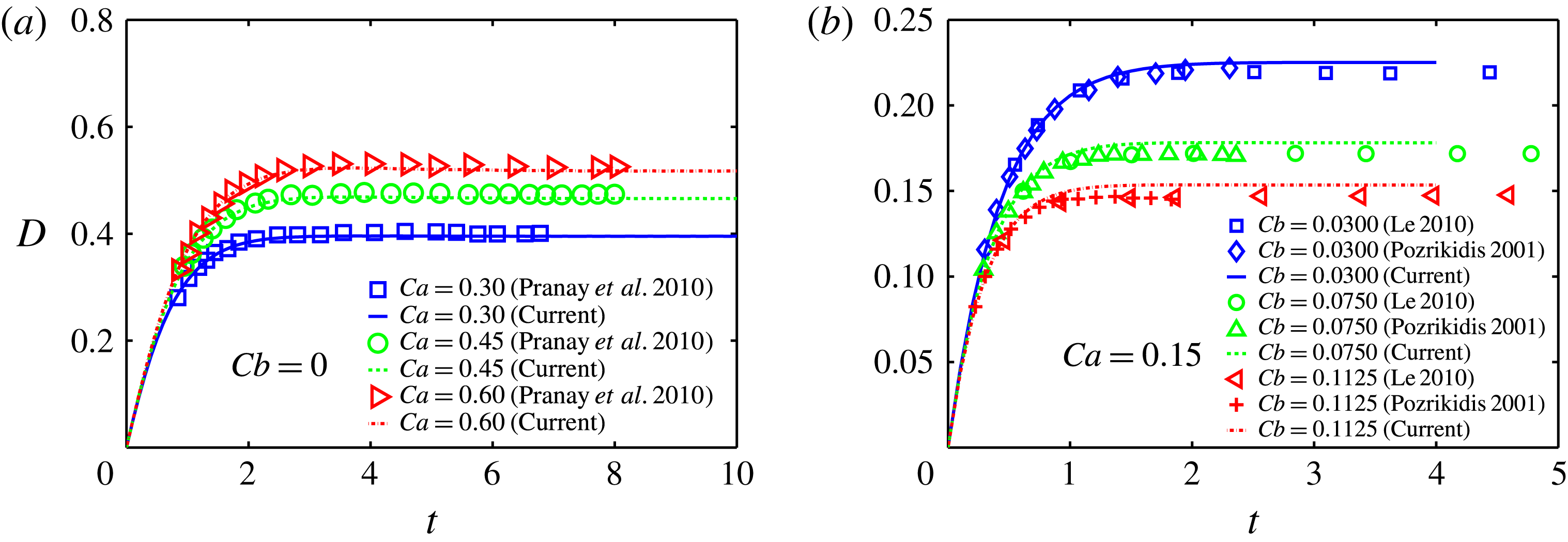
The tank-treading motion of an initially spherical capsule in homogeneous shear flow is selected as the first validation case of our implementation. The capsule evolves into a prolate and reaches a steady deformed shape where the membrane continuously rotates in a tank-treading fashion. The time-dependent capsule deformation is measured by the Taylor parameter
 $$\begin{eqnarray}D=\frac{L_{max}-L_{min}}{L_{max}+L_{min}},\end{eqnarray}$$
where
 $L_{max}$
and
 $L_{min}$
are the maximum and minimum dimensions of the capsule in the shear plane. We display
 $D$
as a function of time for neo-Hookean capsules with a varying
 $\mathit{Ca}$
and no bending stiffness in figure 2(a). Good agreement is observed between our simulations and those of Pranay et al. (Reference Pranay, Anekal, Hernandez-Ortiz and Graham2010).
(a) Variation of the deformation parameter
 $D$
versus time for an initially spherical neo-Hookean capsule in shear flow. Different values of the capillary number
 $\mathit{Ca}$
are chosen. The profile of the capsule in the shear plane is an ellipse with a long axis
 $L_{max}$
and short axis
 $L_{min}$
; the Taylor parameter quantifying the capsule deformation is
 $D=(L_{max}-L_{min})/(L_{max}+L_{min})$
. (b) Same as (a), but with
 $\mathit{Ca}=0.15$
and different values of the reduced bending modulus
 $Cb$
.

We next compare cases including bending modulus against the results of Pozrikidis (Reference Pozrikidis2001) and Le (Reference Le2010), see figure 2(b). The agreement is generally good although small differences appear when the capsule reaches its equilibrium shape. This is probably due to the different discretization used to evaluate the high-order derivatives for the calculation of bending moments. As pointed out by Pozrikidis (Reference Pozrikidis2001), his simulations suffer from ‘significant inaccuracies’ at high capsule deformations; our results agree very well with theirs in the small deformation regime (around
 $t<0.5$
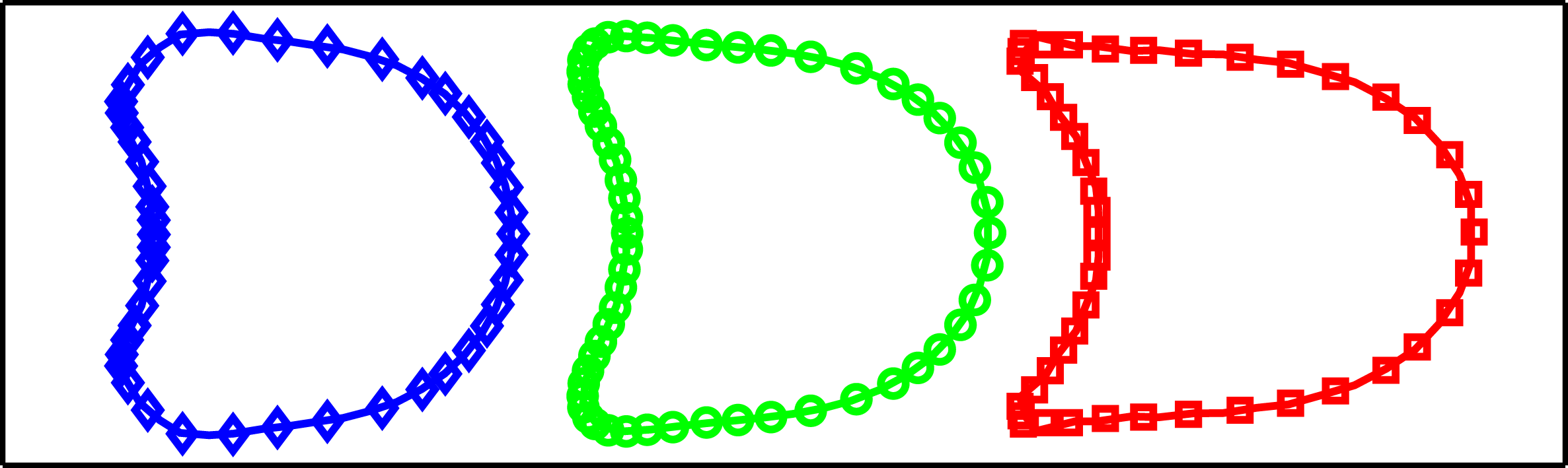
). To verify the nearly singular integration, we therefore also simulate a capsule with zero bending stiffness compressed in a confined square duct, and report excellent agreement with the data of Hu et al. (Reference Hu, Salsac and Barthès-Biesel2011), see figure 3.
Equilibrium profiles of neo-Hookean capsules with different capillary number
 $\mathit{Ca}$
in a square duct of size
 $l_{duct}$
and confinement
 $2a/l_{duct}=0.9$
,
 $Cb=0$
. The symbols correspond to the results of Hu et al. (Reference Hu, Salsac and Barthès-Biesel2011) and the solid lines to our simulations using
 $N_{SH}=24$
modes to represent the membrane surface: ♢,
 $\mathit{Ca}=0.02$
; ○,
 $\mathit{Ca}=0.05$
; ▫,
 $\mathit{Ca}=0.10$
.

3. Results
We consider an initially spherical capsule located at the centre of the square duct, as deformable objects tend to move towards the centreline due to the Fåhraeus effect. We impose the analytical velocity profile of a rectangular duct flow (Spiga & Morino Reference Spiga and Morino1994) at the inlet with mean velocity
 $V_{C}$
. We anchor the centre of the capsule at
 $(0,-5,0)a$
, i.e.
 $5a$
away from both the computational inlet and the corner, and release it after it has reached its equilibrium shape. This distance is large enough for the interaction between the capsule and the inlet/corner to be negligible during this initial phase.
We investigate the influence of the capillary number
 $\mathit{Ca}$
on the dynamics of the capsule, including its deformation, trajectory, velocity, surface area and principal tensions. The reduced bending modulus is fixed to
 $Cb=0.04$
, unless otherwise specified. In addition, we examine the influence of the confinement and of the geometry of the corner.
We note that
 $Cb\approx 0.01$
for RBCs, according to Pozrikidis (Reference Pozrikidis2005a
) and Zhao et al. (Reference Zhao, Isfahani, Olson and Freund2010). We adopt the larger value
 $Cb=0.04$
to prevent the bulking of membrane that would easily destabilize the simulations. Luckily, we found the influence of varying
 $Cb$
is much weaker than that of varying the capillary number
 $\mathit{Ca}$
;
 $Cb$
represents the relative strength of bending over shearing and its variation from 0.01 to 0.04 accounts for only 3 % of the shear modulus.
3.1. Square duct flow with a 90° straight corner
We begin by investigating the motion of a capsule transported in a moderately confined square duct (of width
 $H_{x}=3a$
) with a straight corner. Throughout the work, the cross-section of the vertical and horizontal duct remains the same,
 $H_{y}\equiv H_{x}$
.
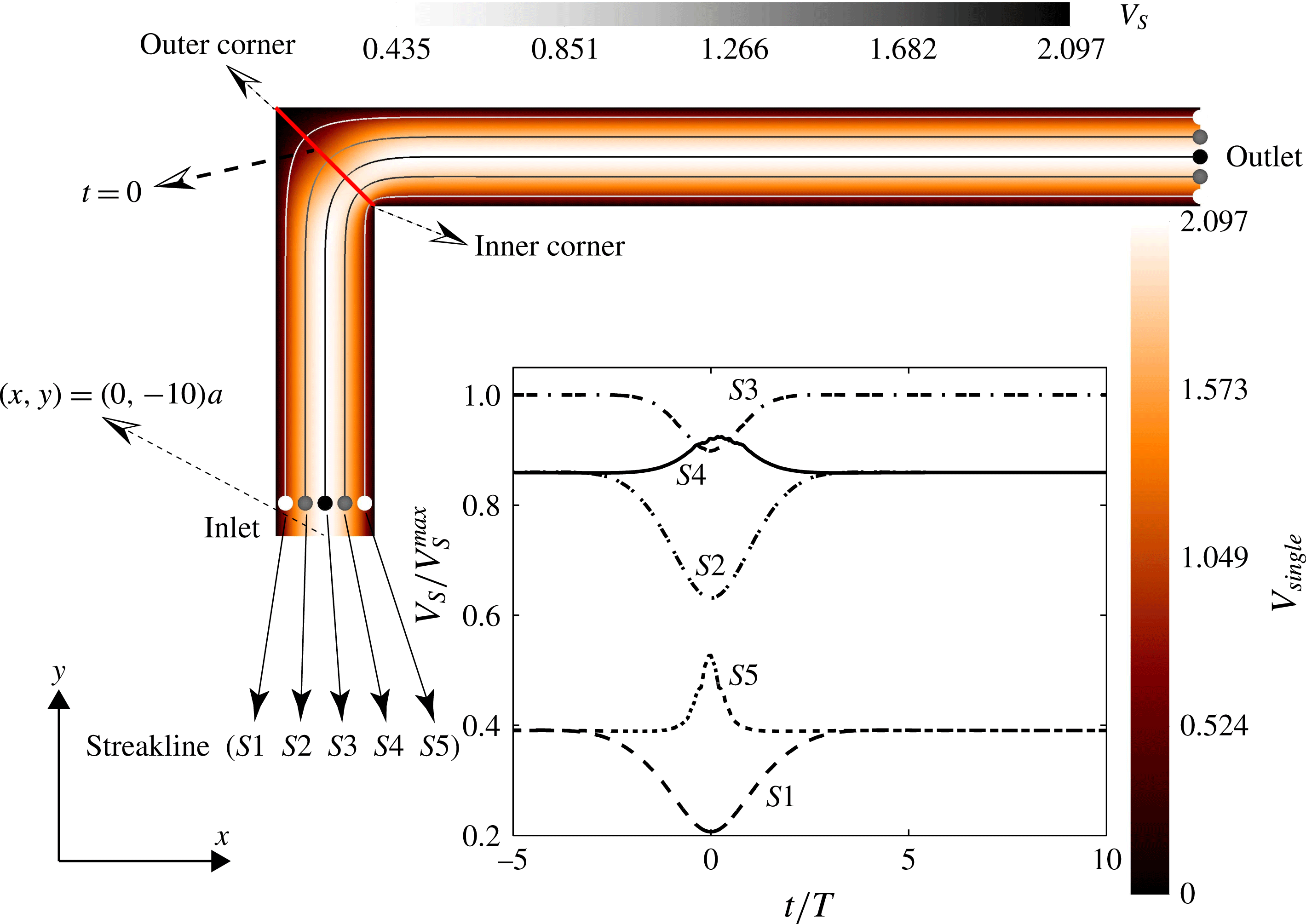
The background flow in the absence of capsules is referred to as the single-phase flow and is illustrated in figure 4 in the
 $x{-}y$
plane. We show five trajectories
 $(S1{-}S5)$
starting from equally spaced points on the line
 $y=-9a,\;x\in [-1.2,1.2]a$
; they are ordered from the outer to the inner corner so that
 $S3$
goes through the centre of the domain. The velocity magnitude
 $V_{S}(t)$
is symmetric about
 $t=0$
: when the minimum is reached for
 $S1$
–
 $S3$
, a maximum occurs for
 $S4$
and
 $S5$
.
The velocity field pertaining the single-phase flow in a square duct of width
 $H_{x}=3a$
with a straight corner. The flow field and streaklines are coloured by their magnitude
 $V_{single}$
and
 $V_{S}$
respectively. The streaklines
 $(S1{-}S5)$
start from points equally spaced between
 $(-1.2,-9)a$
and
 $(1.2,-9)a$
.
 $V_{S}$
divided by the maximum flow velocity is depicted in the inset versus time, where
 $t=0$
corresponds to the time when a fluid particle crosses the corner symmetry axis.

Trajectories and profiles on the
 $x{-}y$
plane of capsules with capillary number (a)
 $\mathit{Ca}=0.075$
and (b)
 $\mathit{Ca}=0.35$
, reduced bending modulus
 $Cb=0.04$
and confinement
 $H_{x}/a=3$
. The shading denotes the initial equilibrium shape. The curve with circles represents the centroid path. The dash–dotted curve is the centreline streakline of the single-phase flow. Dash–dotted curves with filled and hollow diamonds show trajectories of front and rear apices, respectively; dashed curves with squares show that of left and right apices. The dashed arrows connecting the left and right apices indicate the rotation of the membrane.

Time evolution of the velocity of the capsule centre,
 $V_{cap}$
, scaled by the mean velocity
 $V_{C}$
of the duct in (a), and by the cell velocity at equilibrium
 $V_{equ}$
in (b). The confinement
 $H_{x}/a=3$
and results are shown for capsules with
 $\mathit{Ca}=0.0375$
, 0.075, 0.15, 0.3 and 0.35 and a reduced bending modulus
 $Cb=0.04$
. The shape of the capsules at the maximum velocity is provided in (b).

3.1.1. Trajectory of the capsule and membrane rotation
The deformation and trajectories of capsules with
 $\mathit{Ca}=0.075$
and
 $\mathit{Ca}=0.35$
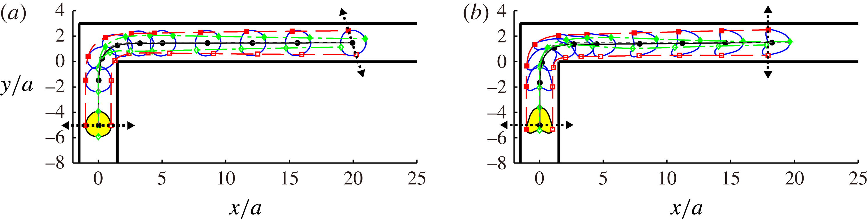
are displayed in figures 5(a) and 5(b), respectively. The centroid trajectory (curve with circles) closely matches the middle streakline
 $S3$
(dash–dotted curve) and is almost insensitive to the membrane elasticity. We also mark and trace the four apices of the capsule from the equilibrium shape. For
 $\mathit{Ca}=0.075$
, we identify a clear rotation by comparing the initial and final positions of the apices. The front and rear apices initially on
 $S3$
follow trajectories (indicated by filled and hollow diamonds respectively) deviating from
 $S3$
significantly; the front/rear apex drifts towards the outer/inner corner, eventually remaining above/below the centroid trajectory. The left/right apex starts from the same vertical position and approximately moves along the streakline
 $S1/S5$
. These are characterized by a decreasing/increasing velocity around the corner (see figure 4); as a result, the right apex travels beyond the left, as shown in figure 5. The material points on the capsule rotate, therefore, in the anti-clockwise direction. This rotation is induced by the flow near the corner: this is spatially non-uniform across the duct and the material points near the inner/outer corner are advected by the accelerating/decelerating flow, which results in a net membrane rotation. In the case of
 $\mathit{Ca}=0.35$
, the membrane rotation is not as clear. Compared to the case with
 $\mathit{Ca}=0.075$
, the right apex is closer to the wall where the underlying flow is slower, thus compensating the increase of the fluid velocity near the corner. Hence, the left and right apices are roughly found at the same streamwise location downstream of the corner.
3.2. Velocity of the capsule
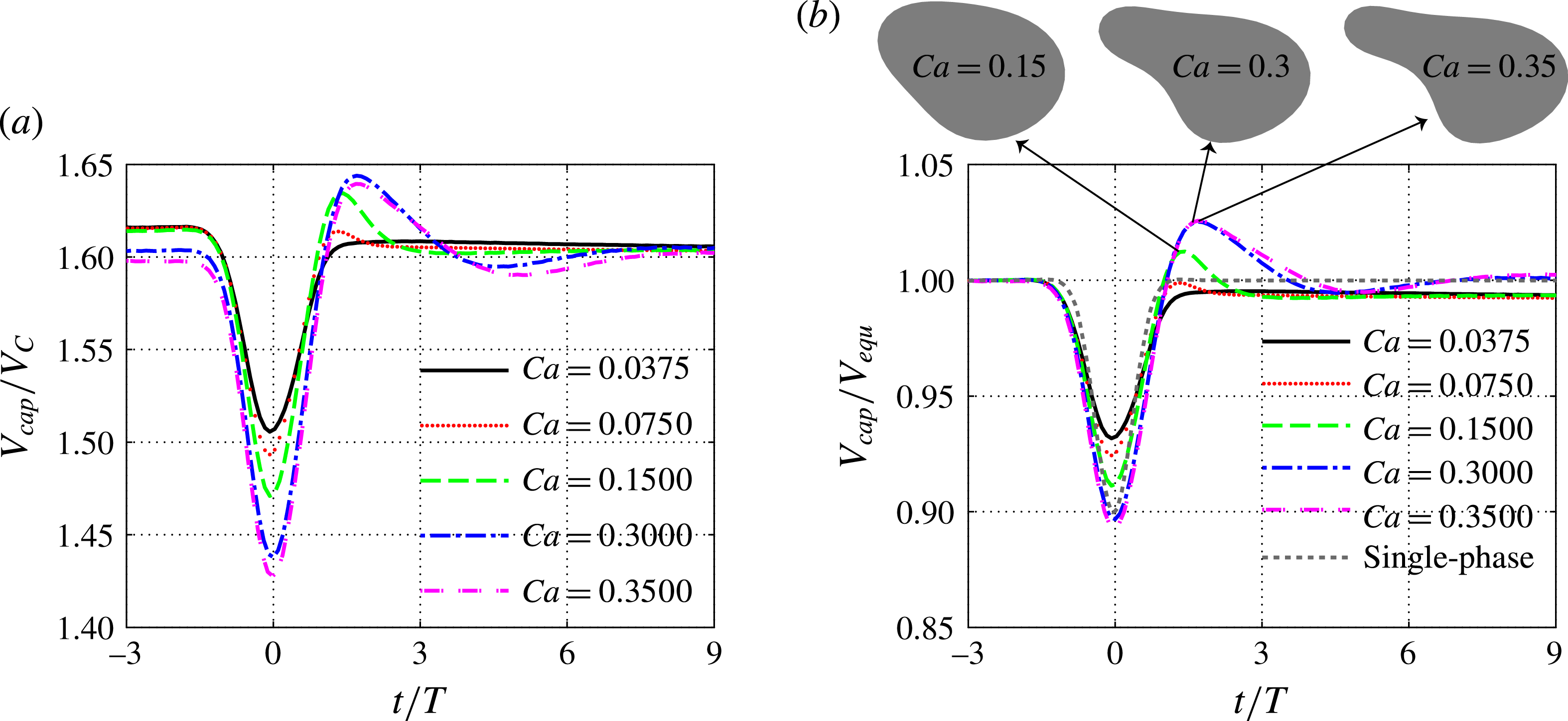
The velocity of the capsule centre,
 $V_{cap}$
, scaled by the mean velocity
 $V_{C}$
is reported in figure 6(a) as a function of time; the same quantity instead divided by the equilibrium velocity
 $V_{equ}$
, is depicted in figure 6(b), together with the velocity on the centre streakline
 $S3$
of the single-phase flow (cf. figure 4). All capsules move faster than the average flow velocity, a signature of the Fåhraeus effect. Note that the equilibrium velocity
 $V_{equ}$
, the velocity in a straight duct, decreases slightly with
 $\mathit{Ca}$
. This was also discussed by Kuriakose & Dimitrakopoulos (Reference Kuriakose and Dimitrakopoulos2011) (figure 8a in their paper):
 $V_{equ}$
increases with
 $\mathit{Ca}$
as
 $H_{x}/a=2.5$
but decreases in the less confined case,
 $H_{x}/a=10/3$
; our simulations with
 $H_{x}/a=3$
are between the two cases in Kuriakose & Dimitrakopoulos (Reference Kuriakose and Dimitrakopoulos2011) and confirm the negative trend of
 $V_{equ}$
at low confinement. The velocity of the capsule is related to the thickness of the capsule–wall lubrication film; a thinner film induces higher viscous dissipation and thus reduces the capsule velocity; the thickness of the film when the capsule is slower (
 $\mathit{Ca}=0.35$
), is about 93 % that of the fast capsule (
 $\mathit{Ca}=0.0375$
).
The velocity of the capsule decreases when approaching the corner and increases when leaving it, reflecting the behaviour of the background flow; the time histories reveal a minimum located at
 $t=0$
, when the particle centre is on the corner axis. This minimum velocity decreases with the capillary number
 $\mathit{Ca}$
; a slightly thinner lubrication film is observed at the corner axis as
 $\mathit{Ca}$
changes from 0.35 to 0.075 (see figure 5). Unlike the underlying flow, the motion of the capsule clearly breaks the time-reversal symmetry about
 $t=0$
, revealing an overshoot during the recovery stage; this symmetry breaking becomes more evident for higher
 $\mathit{Ca}$
. This loss of symmetry is related to the viscoelasticity induced by the fluid–capsule interaction.
We show the shape of the capsule associated with the larger velocity overshoots (
 $\mathit{Ca}=0.15$
, 0.3 and 0.35) in figure 6(b) at the time the peak velocity is attained. A clear tail-like protrusion is observed for the two largest
 $\mathit{Ca}$
, due to the streamwise stretching induced by the background accelerating flow. Such a shape is responsible for the observed velocity overshoot, as the streamwise membrane extension corresponds to a decrease of the cross-flow extension of the capsule (its volume must be conserved). This causes a larger distance between capsule and wall and a reduced viscous dissipation. Not surprisingly, as the capsule leaves the corner, its vertical dimension recovers to the equilibrium value and so does the velocity.
The velocity does not converge exactly to its equilibrium value: a maximum relative difference of around
 $0.6\,\%$
is observed. It would require a prohibitively long computational domain and integration time to obtain a precise convergence as also observed by Woolfenden & Blyth (Reference Woolfenden and Blyth2011); the physics of the final capsule relaxation is therefore beyond the scope of the present investigation.
Time evolution of the non-dimensional surface area for the same capsules in figure 6. (a) Total surface area
 $A/4{\rm\pi}a^{2}$
and (b) projected area on the
 $x{-}y$
plane
 $A_{xy}/{\rm\pi}a^{2}$
);
 $A_{equ}$
and
 $A_{peak}$
indicate the equilibrium and peak value of
 $A$
respectively. Solid circles indicate the time
 $t|A_{xy}^{min}/T$
when the minimum area
 $A_{xy}$
is achieved. The inset of (b) shows
 $t|A_{xy}^{min}/T$
versus
 $\mathit{Ca}$
.

3.3. Capsule surface area and deformation
The capsule surface area,
 $A$
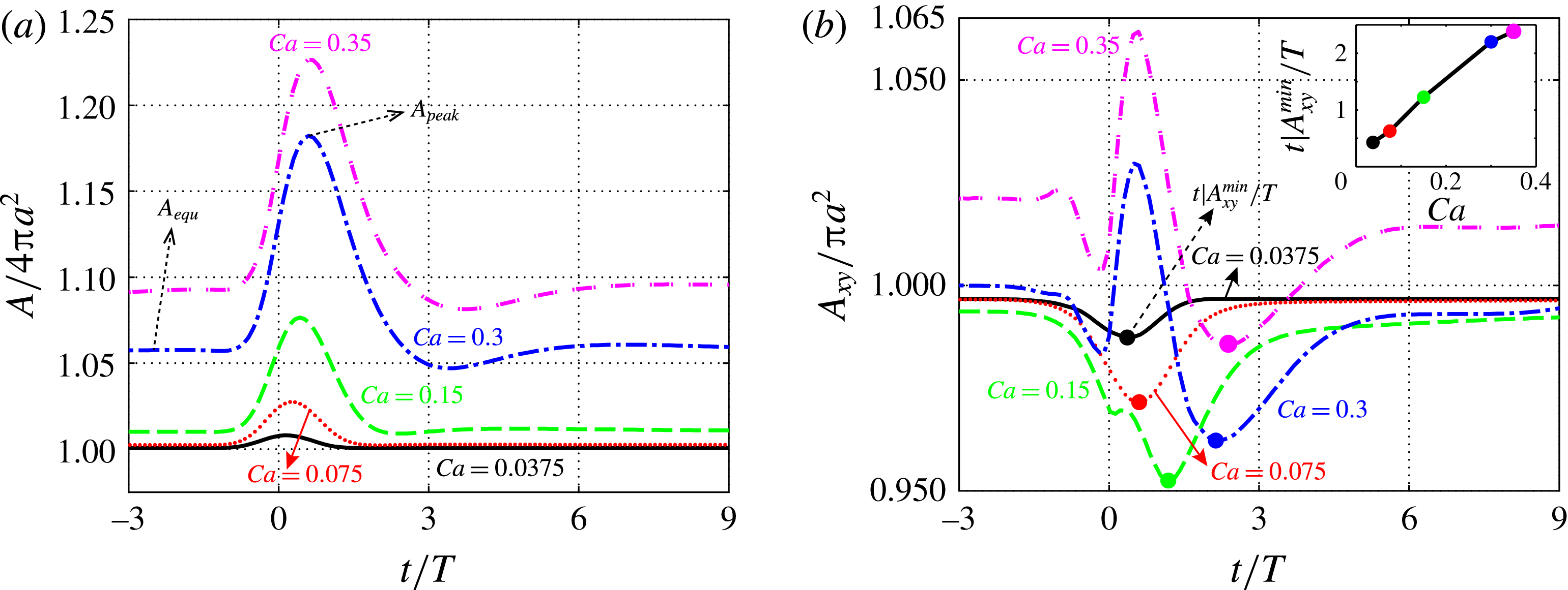
, is used as indicator of the global deformation. This is reported in figure 7 for the same cases as in figure 6. When the capsule is far away from the corner, the area maintains the equilibrium value
 $A_{equ}$
, an increasing function of
 $\mathit{Ca}$
. The area variation
 $A_{equ}/4{\rm\pi}a^{2}-1$
is almost zero for the cases with
 $\mathit{Ca}=0.0375$
and 0.075, whereas it grows to values around 0.1 when
 $\mathit{Ca}=0.35$
. As the capsule travels around the corner, the deformation reaches its peak value and its variation
 $A_{peak}/4{\rm\pi}a^{2}-1$
is around 0.2 for the highest
 $\mathit{Ca}$
investigated.
Ideally, the dependence of the area on the capillary number can be used to deduce the membrane properties of capsules, as shown by Lefebvre et al. (Reference Lefebvre, Leclerc, Barthès-Biesel, Walter and Edwards-Lévy2008), Chu et al. (Reference Chu, Salsac, Leclerc, Barthès-Biesel, Wurtz and Edwards-Lévy2011) and Hu et al. (Reference Hu, Sévénié, Salsac, Leclerc and Barthès-Biesel2013), who focus on the identification based on deformation. However, direct measurement of the total surface area is not easy, while it is more feasible to measure its two-dimensional projection. As a consequence, we display the projection of the capsule area on the
 $x{-}y$
mid-plane in figure 7(b).
The projected area
 $A_{xy}$
varies with time and cell deformability in a more complicated way. For the two smallest values of
 $\mathit{Ca}$
,
 $A_{xy}$
reaches the minimum around
 $t=0$
before recovering to the equilibrium value past the corner. The cases characterized by
 $\mathit{Ca}=0.3$
and 0.35 display a clear peak in deformation right after
 $t=0$
, with two sharp troughs, one before and one after. This wavy variation is already visible when
 $\mathit{Ca}=0.15$
, although weak. Further examination of the behaviour in the range
 $\mathit{Ca}\in [0.15,0.3]$
confirms that the time traces of the area deformation become more wavy as
 $\mathit{Ca}$
increases; more elastic material is prone to exhibit more oscillatory motions under the same excitation, the spatially developing flow here. The inset of figure 7(b) shows the time
 $t|A_{xy}^{min}/T$
corresponding to the minimum projected area
 $A_{xy}$
. This can be regarded as the phase lag of the capsule and it increases almost linearly with
 $\mathit{Ca}$
.
3.4. Principal tension on the capsule
The tension developing on the membrane is of great importance since it influences the release of molecules (Goldsmith et al.
Reference Goldsmith, Bell, Braovac, Steinberg and McIntosh1995) and ATP (Wan, Ristenpart & Stone Reference Wan, Ristenpart and Stone2008) by RBCs and causes haemolysis, to cite two examples. We analyse the principal tension
 ${\it\tau}_{i}^{P}\;(i=1,2)$
, to better understand the potential mechanical damage of capsules passing through a corner. For any definition of strain energy function
 $W_{S}(I_{1},I_{2})$
, the
 ${\it\tau}_{i}^{P}$
are derived as (Skalak et al.
Reference Skalak, Tozeren, Zarda and Chien1973):
 $$\begin{eqnarray}\displaystyle & \displaystyle {\it\tau}_{1}^{P}=2\frac{{\it\lambda}_{1}}{{\it\lambda}_{2}}\left(\frac{\partial W_{S}}{\partial I_{1}}+{\it\lambda}_{2}^{2}\frac{\partial W_{S}}{\partial I_{2}}\right)\!, & \displaystyle\end{eqnarray}$$
 $$\begin{eqnarray}\displaystyle & \displaystyle {\it\tau}_{2}^{P}=2\frac{{\it\lambda}_{2}}{{\it\lambda}_{1}}\left(\frac{\partial W_{S}}{\partial I_{1}}+{\it\lambda}_{1}^{2}\frac{\partial W_{S}}{\partial I_{2}}\right)\!. & \displaystyle\end{eqnarray}$$
 $\max ({\it\tau}_{1}^{P}(\boldsymbol{x},t),{\it\tau}_{2}^{P}(\boldsymbol{x},t))$
and the isotropic principal tension
 $({\it\tau}_{1}^{P}(\boldsymbol{x},t)+{\it\tau}_{2}^{P}(\boldsymbol{x},t))/2$
; their surface maxima
 ${\it\tau}_{max}^{P}(t)$
and
 ${\it\tau}_{max}^{P_{ISO}}(t)$
are defined as
 $$\begin{eqnarray}\displaystyle & \displaystyle {\it\tau}_{max}^{P}(t)=\max _{\boldsymbol{x},i=1,2}({\it\tau}_{i}^{P}(\boldsymbol{x},t)), & \displaystyle\end{eqnarray}$$
 $$\begin{eqnarray}\displaystyle & \displaystyle {\it\tau}_{max}^{P_{ISO}}(t)=\max _{\boldsymbol{x}}(({\it\tau}_{1}^{P}\left(\boldsymbol{x},t\right)+{\it\tau}_{2}^{P}(\boldsymbol{x},t))/2), & \displaystyle\end{eqnarray}$$
 $(t)$
will be omitted hereinafter for the sake of clarity.
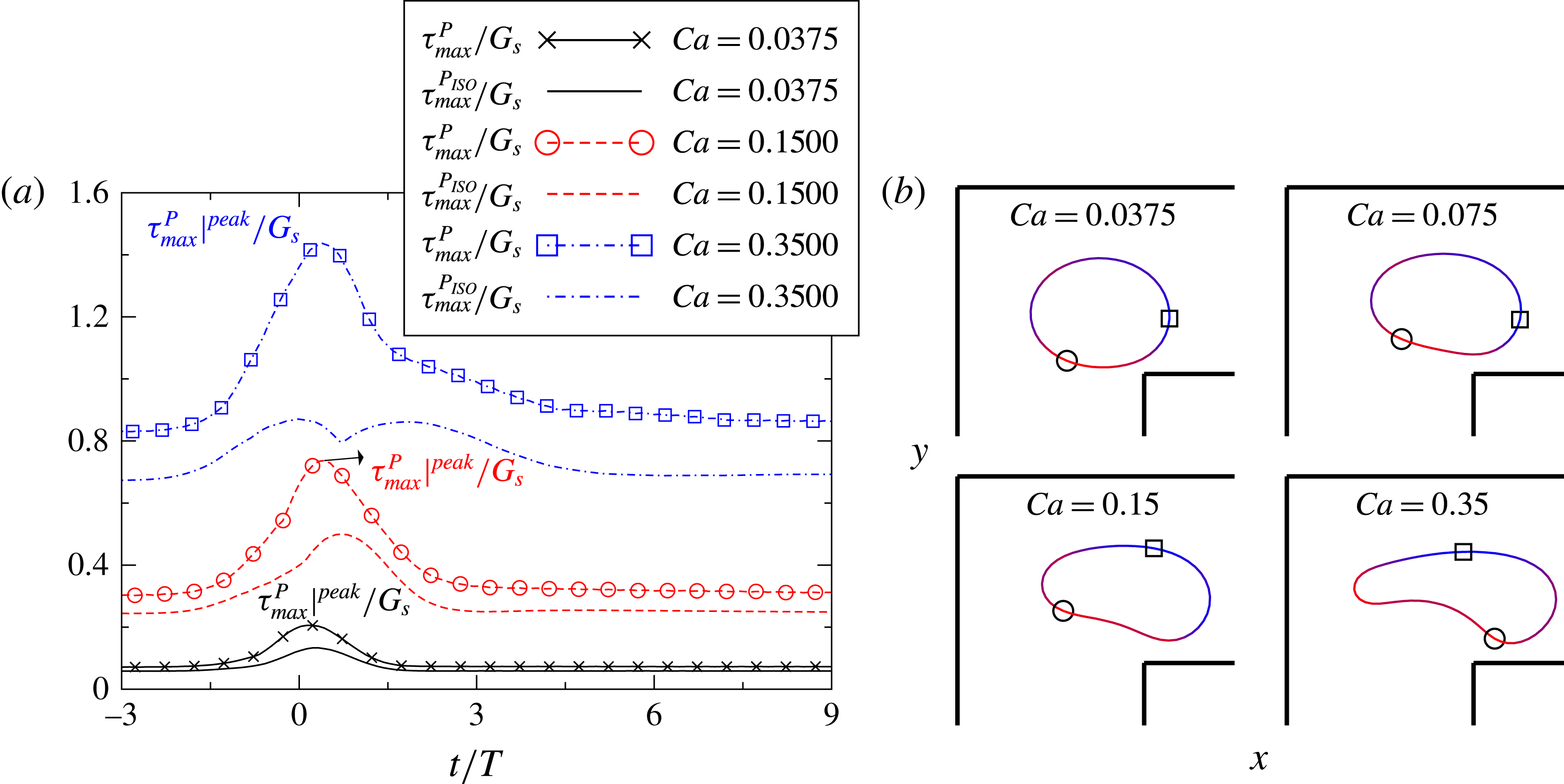
The temporal evolution of
 ${\it\tau}_{max}^{P}/G_{s}$
and
 ${\it\tau}_{max}^{P_{ISO}}/G_{s}$
is shown in figure 8 for capsules going through a straight corner. For most cases, both quantities increase monotonically with
 $\mathit{Ca}$
, reaching the peak values slightly after the corner before relaxing back to the equilibrium value. The difference between the two tensions is more pronounced at the corner,
 ${\it\tau}_{max}^{P}/{\it\tau}_{max}^{P_{ISO}}\approx 2$
, and weak in the straight ducts. We also show in the figure the shape of some capsules when the maximum major principal tension is reached, with the minimum and maximum of
 ${\it\tau}_{max}^{P}$
indicated by a circle and square respectively. The maximum of
 ${\it\tau}_{max}^{P}$
develops at the front for the capsules with
 $\mathit{Ca}=0.0375,0.075$
, while it moves to the top part for
 $\mathit{Ca}=0.35$
. Material points are prone to accumulate at the rear of the capsule and the principal tension is therefore relatively low. As
 $\mathit{Ca}$
increases, the rear part of the capsule changes from a convex to concave shape, something more evident for the case
 $\mathit{Ca}=0.35$
.
(a) Time evolution of the maximum of the two principal tensions in the non-dimensional form,
 ${\it\tau}_{max}^{P}/G_{s}$
and
 ${\it\tau}_{max}^{P_{ISO}}/G_{s}$
, for the major and isotropic principal tension respectively. (b) Position and contour of the capsules on the
 $x{-}y$
plane when reaching the maximum major principal tension
 ${\it\tau}_{max}^{P}|^{peak}$
. The magnitude of
 ${\it\tau}_{max}^{P}$
is indicated by light grey/dark grey (red and blue online) for low/high values and its minimum/maximum position by the circle/square.

3.5. The influence of confinement and geometry of the corner
We examine first the influence of confinement on the capsule motion by varying the width
 $H_{x}/a$
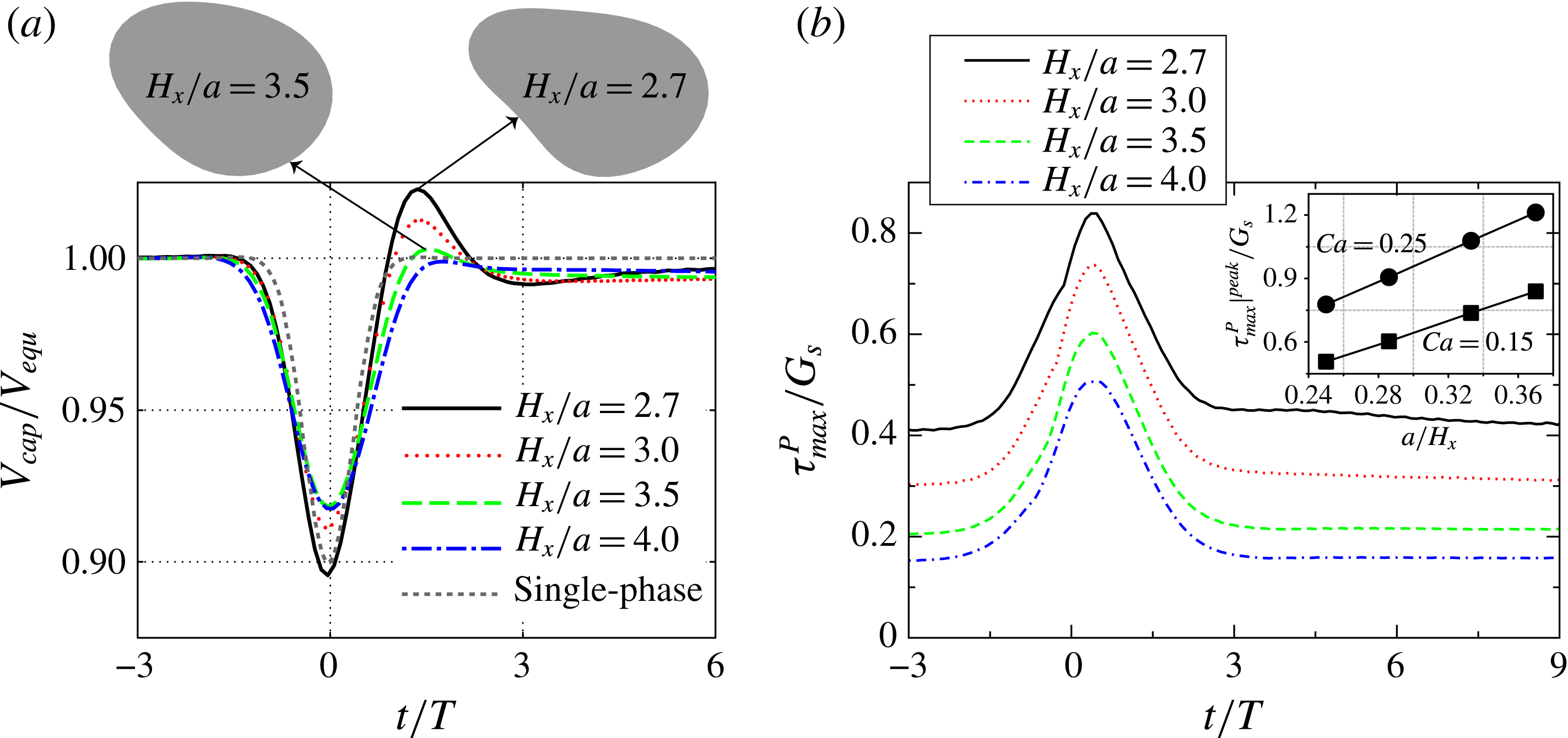
from 2.7 to 4. The velocity of the capsule, divided by its equilibrium velocity, is shown in figure 9 for
 $\mathit{Ca}=0.15$
. The time-symmetry around
 $t=0$
is almost preserved for the least confined case
 $H_{x}/a=4$
. As the confinement increases, the symmetry breaking discussed before and the corresponding velocity overshoot become more apparent. These are associated with a decrease of the minimum velocity at the corner. As
 $H_{x}/a$
varies from 3.5 to 2.7, the velocity overshoot also clearly increases. The shape of the capsule at the time of maximum velocity is also displayed in the figure. The capsule with highest velocity is more elongated and has a larger distance from the wall (lower lubrication friction), in analogy to the observations in § 3.2 for capsules of different elasticity.
Time evolution of (a) the velocity
 $V_{cap}/V_{equ}$
and (b) the major principal tension
 ${\it\tau}_{max}^{P}/G_{s}$
for
 $\mathit{Ca}=0.15$
where the width of the square duct is varied from
 $H_{x}/a=2.7$
to
 $H_{x}/a=4$
. The shape of the capsule at the time when the maximum velocity is attained is also given in (a). The inset of (b) shows the relation between the maximum major principal tension
 ${\it\tau}_{max}^{P}|^{peak}/G_{s}$
and the inverse of the duct width
 $a/H_{x}$
for
 $\mathit{Ca}=0.15$
and 0.25.

The surface maximum of the non-dimensional major principal tension
 ${\it\tau}_{max}^{P}/G_{s}$
is depicted in figure 9(b) for the same cases:
 ${\it\tau}_{max}^{P}$
increases monotonically with the confinement. The maximum over time of
 ${\it\tau}_{max}^{P}|^{peak}/G_{s}$
is displayed versus
 $a/H_{x}$
for
 $\mathit{Ca}=0.15$
and 0.25 in the inset of the same figure to show that the peak principal tension increases linearly with
 $a/H_{x}$
. This relationship may be useful to estimate the mechanical stress on/damage to the cells in micro-fluidic devices during the design stage.
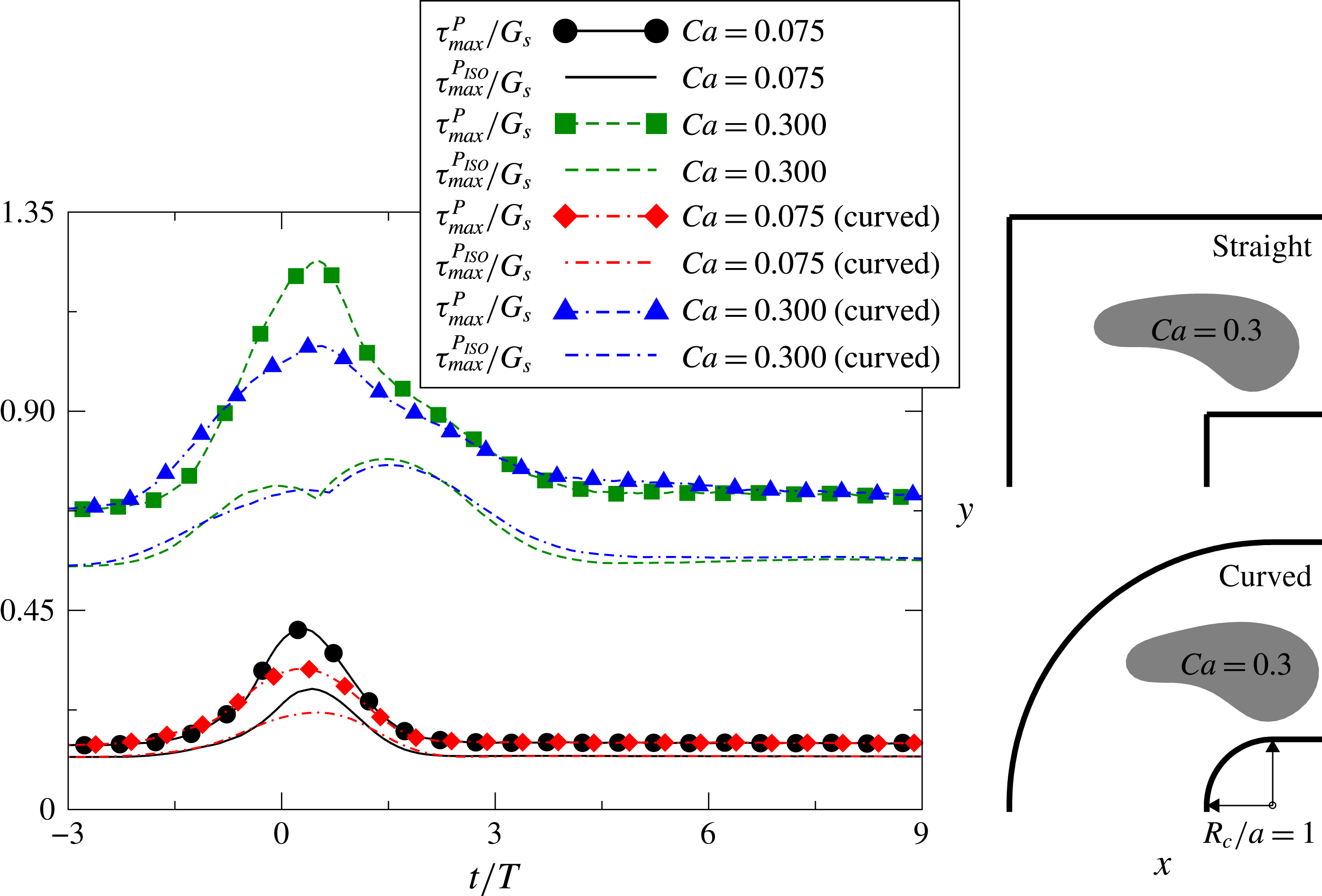
Finally, we consider a curved corner with inner radius
 $R_{c}/a=1$
. In figure 10 we compare the principal tensions on the membrane with those in the straight corner for capillary numbers
 $\mathit{Ca}=0.075$
and 0.3. Except for the isotropic principal tension of the capsule with
 $\mathit{Ca}=0.075$
, the principal tension decreases significantly in the curved corner.
Time evolution of the major principal tension
 ${\it\tau}_{max}^{P}/G_{s}$
for capsules
 $\mathit{Ca}=0.075/0.3$
through a straight and a curved corner. The curvature radius of the curved corner is
 $R_{c}/a=1$
. The shape of capsule on the
 $x{-}y$
plane is shown when it reaches the peak
 ${\it\tau}_{max}^{P}$
.

4. Discussion and conclusion
We investigate the motion of a three-dimensional deformable capsule, whose membrane obeys the neo-Hookean constitutive relation, in a square duct flow with a corner. We present in this work a new implementation of the BIM accelerated by the GGEM, the general-geometry Ewald method, to resolve fluid–structure interactions at low Reynolds number in complex geometries. The algorithm is coupled with a spectral method based on spherical harmonics for the membrane dynamics. In this section, we first discuss the details of the numerical method, followed by a short summary of the main physical findings.
The GGEM shares similarities with the classic immersed boundary methods (IBM) (Mittal & Iaccarino Reference Mittal and Iaccarino2005). Both approaches require a Lagrangian mesh for the suspended objects and an Eulerian (typically Cartesian) mesh for the fluid; the Dirac delta function, representing the localized forcing from the object, is approximated numerically. In the IBM, the localized force is spread from each Lagrangian point onto a number of surrounding Eulerian points to enforce the desired boundary conditions at the fluid/solid interface. The accuracy of IBM degenerates if close hydrodynamic interactions arise, which may require ad hoc corrections to account for the correct lubrication forces (Lashgari et al. Reference Lashgari, Picano, Breugem and Brandt2014). As shown in (2.5), the Dirac delta function is also smeared in the local problem of GGEM, but its singular behaviour can be solved accurately by boundary integral techniques with singular integration. If a regularized-Stokeslet technique is instead employed as in Pranay et al. (Reference Pranay, Anekal, Hernandez-Ortiz and Graham2010) and Hernández-Ortiz et al. (Reference Hernández-Ortiz, de Pablo and Graham2007), the GGEM closely resembles an IBM as proved by Pranay et al. (Reference Pranay, Anekal, Hernandez-Ortiz and Graham2010). Note also that a traditional IBM requires a uniform Eulerian grid to conserve the moments of the force and sophisticated treatments are needed to adapt IBM to a non-uniform and/or unstructured grid as done by Pinelli et al. (Reference Pinelli, Naqavi, Piomelli and Favier2010) and Mendez, Gibaud & Nicoud (Reference Mendez, Gibaud and Nicoud2014) among others. One advantage of the GGEM is that the smoothing of the local forcing is exactly compensated by the global forcing due to the linearity of Stokes equations. The integral of the force field and its moments are therefore preserved. Hence, Stokes solvers based on uniform or non-uniform grids can be readily coupled to the GGEM. In our case, the Eulerian grid points (GLL points) are non-uniformly distributed as shown in figure 1.
GGEM was originally designed to resolve the hydrodynamic interaction among multiple particles in Stokes flows. Suppose that there are
 $N^{p}$
particles and each of them is discretized into
 $M$
Lagrangian points, then the total number of points is
 $N^{p}M$
and the number of degrees of freedom
 $N_{d}\sim N^{p}M$
. For traditional non-accelerated BIM, the number of operations required to form the mobility matrix scales with
 $N_{d}^{2}$
. This poses the major difficulty in applying BIM to a large number of particles. Accelerating techniques for BIM have thus been developed to overcome this restriction, and GGEM is one of them. The decomposition of the Dirac delta function into two parts reduces the number of operations from
 $O(N_{d}^{2})$
to
 $O(N_{d})$
or
 $O(N_{d}\log N_{d})$
(Hernández-Ortiz et al.
Reference Hernández-Ortiz, de Pablo and Graham2007). The modified Green’s function for the local problem is designed such that the local solution decays exponentially over a distance of about
 ${\it\alpha}_{cut}^{-1}$
. Neglecting interactions that occur beyond the cut-off distance
 $R_{cut}\sim {\it\alpha}_{cut}^{-1}$
, the number of operations for the local solution decreases and scales linearly with
 $N_{d}$
. The scaling of the global problem depends on the mesh-based solver, as well as the geometry and boundary conditions of the computational domain. The solver used here, NEK5000, is computationally more expensive than Fourier-based methods such as those used in Kumar & Graham (Reference Kumar and Graham2012), but it allows for arbitrary geometries and is highly parallel.
It is hard to provide a scaling for the global part of the problem in general geometries; however, the advantage of a numerical approach like that pursued here relies on two points: (i) GGEM provides a convenient way to reshape the
 $O(N_{d}^{2})$
long-ranged interactions and pack them into a problem solvable by a mesh-based solver; (ii) a highly parallel solver is chosen to considerably reduce the computational time. Note that a naive parallelization of traditional BIM implementations is not possible for a large
 $N_{d}$
due to the prohibitively large amount of memory needed and poor scalability of the linear system with a dense matrix. It should be noted that our implementation might be less efficient than traditional BIM for studying the dynamics of one (as we do here) or a few capsules. This is, however, our first step in the development of a computational framework for suspensions of deformable/rigid particles in general geometries.
This numerical approach is used here to examine the motion of a capsule through a square duct with a corner, focusing on its trajectory, velocity, deformation, total and projected surface area, and principal tension. We aim to better understand the transient dynamics of capsules in a micro-fluidic device with realistic geometries.
We study the deformation of the capsules when varying the capillary number, the ratio of viscous to elastic forces. The capsule trajectories closely follow the underlying flow and are therefore rather insensitive to how the capsules deform. Due to the strong confinement, deviations from the underlying streamline require a significant viscous dissipation. Conversely, the deformability of a capsule closely influences its shape, velocity and the mechanical stress developing on the membrane as documented in the results section.
The corner flow can be potentially adopted to infer the material properties of deformable particles as shown by Lefebvre et al. (Reference Lefebvre, Leclerc, Barthès-Biesel, Walter and Edwards-Lévy2008) and Chu et al. (Reference Chu, Salsac, Leclerc, Barthès-Biesel, Wurtz and Edwards-Lévy2011) using straight tube or channel flows. Unlike these works, transient effects are present in the flow past a corner because of its spatial inhomogeneity. When the capsule is far away from the corner, the surface area, velocity and principal tension reach equilibrium values that are a function of the capillary number
 $\mathit{Ca}$
. When flowing around the corner, the membrane area and tension reach their maxima while the velocity is at its minimum; these extrema are shown here to clearly depend on
 $\mathit{Ca}$
. By utilizing a spatially developing flow, the shape and/or velocity of the capsules can be measured not only at the equilibrium state but also during the transient motions. More robust and accurate inverse methods may be developed using measurements of the extrema values. We further note that a new time scale is introduced in the corner flow, hence the phase lag of the capsule can be identified as illustrated by the temporal evolution of the projected area (see figure 7
b); this quantity indicating the viscoelasticity of capsule is not accessible from traditional steady flow experiments. The spatially developing flow provides supplemental information characterizing the material properties of natural and synthetic cellular structures.
The capsule shape is also closely linked to its velocity. For low
 $\mathit{Ca}$
, the velocity is similar to that of the underlying flow, with an almost perfect time-reversal symmetry; as
 $\mathit{Ca}$
increases, i.e. more pronounced deformations, this symmetry is broken and a velocity overshoot appears past the corner. The streamwise elongation of the capsule increases the capsule–wall distance, and the corresponding lower viscous dissipation can explain the higher capsule velocity.
The surface maxima of the major and isotropic principal tension become significantly different only when the capsule is flowing around the corner. During this time, the maximum major principal tension appears at the front of capsules for configurations with low
 $\mathit{Ca}$
, and shifts towards the outer edge as
 $\mathit{Ca}$
increases.
We have also examined the influence of confinement and of the geometry of the corner. We identify a positive correlation between the asymmetry of the velocity profile and the level of confinement. The peak of the major principal tension increases linearly with the inverse of the duct width
 $a/H_{x}$
. Finally, we show that a curved corner reduces the major principal tension and the deformation of the capsule. We believe the present work can improve our understanding of the capsule motion in complex geometries and support the design of micro-fluidic devices with multiple corners and branches.
Acknowledgements
We thank Professors D. Barthès-Biesel, M. D. Graham and J. B. Freund and Dr H. Zhao for useful discussions. Funding by VR (the Swedish Research Council), the Linné FLOW Centre at KTH and computer time via SNIC (Swedish National Infrastructure for Computing) and HPC at EPFL are greatly acknowledged. L.Z. acknowledges the financial support from the European Research Council (ERC) grant ‘simcomics-280117’ as a postdoc researcher at EPFL where part of the work is performed. This research is also supported by the ERC grant ‘2013-CoG-616186, TRITOS’ to L.B.