

1 Introduction
Wave breaking plays a vital role in enhancing the transfer of mass, momentum and energy across the air–sea interface. Wave breaking is also an important contributor to mixing surface water, generating currents, limiting the wave heights and dissipating wave energy. Exchange of gas across the air–sea interface may be enhanced by air entrainment (Farmer, McNeil & Johnson Reference Farmer, McNeil and Johnson1993) under breaking waves. Breaking-induced air entrainment and associated bubbles also have significant environmental impacts through producing marine aerosols (Blanchard & Woodcock Reference Blanchard and Woodcock1957), as well as scavenging organic material and bacteria from the water column and transporting them to the surface (Blanchard & Syzdek Reference Blanchard and Syzdek1970).
A spilling breaker is typically initiated by the formation of a small region on the forward side of the crest where the water surface becomes rough and then this small region grows by spreading downslope, eventually engulfing most of the forward wave face and forming a turbulent flow (Mason Reference Mason1952). Despite their more frequent occurrences in the open ocean, there exists a relatively smaller number of detailed studies (i.e. featuring flow velocity and/or void fraction) exclusively focusing on (strong) spilling breaking waves when compared with those focusing on plunging breaking waves because of their less dramatic nature. On the other hand, we are aware that there exist many laboratory studies that feature both plunging and spilling breaking waves but focus on specific flow properties (geometry, breaking onset criteria, dissipation, void fraction), let alone measurements of both flow velocities and void fraction. A general consensus is that any type of breaking wave is an important contributor to turbulence, spray and bubble generation at the water surface (Duncan Reference Duncan2001). In the past, studies of spilling breaking waves have been conducted both numerically and experimentally and often compared to those of plunging breaking waves. Visual observations by Rapp & Melville (Reference Rapp and Melville1990) showed that the evolving pattern of the aerated region in spilling breakers is similar in both shallow surf-zone waves and deep-water waves. Ting & Kirby (Reference Ting and Kirby1994, Reference Ting and Kirby1995, Reference Ting and Kirby1996) and Ting (Reference Ting2001) showed, based on laboratory experiments, that turbulent kinetic energy is transported shoreward by plunging breakers and seaward by spilling breakers. Stansby & Feng (Reference Stansby and Feng2005) suggested that the phenomenon could be attributed to the hypothesis that turbulence is more concentrated in the roller for plunging breakers featuring prominent shoreward motion but more distributed for spilling bores. Cowen et al. (Reference Cowen, Sou, Liu and Raubenheimer2003) found that turbulent Reynolds stresses in the swash zone exhibit similarity between plunging and spilling breakers.
One focus in the study of spilling breaking waves is the crest evolution close to the onset of breaking. The onset in spilling breakers is not as well defined as that in the plunging waves, in which the moment when the front face of the crest becomes vertical has been defined as the breaking onset. Duncan et al. (Reference Duncan, Philomin, Qiao and Kimmel1994, Reference Duncan, Qiao, Philomin and Wenz1999) investigated the evolution of the crest near the onset of breaking under very weak spilling breakers generated by dispersive focusing through a series of experiments. For the very weak spilling breakers that are gravity- and surface-tension-dominated, the crest profile just before the onset of turbulent flow is independent of wave frequency (Duncan et al. Reference Duncan, Qiao, Philomin and Wenz1999). The observation is in agreement with the numerical results in Longuet-Higgins (Reference Longuet-Higgins1996). The effect of surface tension has also been investigated due to its role in altering the crest deformation; the effect becomes increasingly important as the wavelength and intensity of the breaker decrease (Duncan Reference Duncan2001). In these surface-tension-dominated cases, the crest deforms, generating a bulge–capillary structure where turbulence is produced at the area of high upward surface curvature at the leading edge of the bulge (Duncan Reference Duncan2001). On the other hand, detailed experimental studies on spilling breaking waves with a longer wavelength, so that the surface tension effect is less important, have been relatively rare.
Past the onset of breaking, the flow entrains air and then quickly turns into a turbulent flow. In the flow, coherent structures have been shown to be capable of transporting momentum and affecting the overall dynamics. Nadaoka, Kino & Koyano (Reference Nadaoka, Kino and Koyano1989) showed that large-scale eddy motion in breaking waves is responsible for the excessive mass flux and enhanced momentum transport. Wavelet-based methods have been proven as an effective way to detect the coherent structures under breaking waves (Govender, Mocke & Alport Reference Govender, Mocke and Alport2004; Longo Reference Longo2009; Huang, Hwung & Chang Reference Huang, Hwung and Chang2010; Na et al. Reference Na, Chang, Huang and Lim2016). The educed length scale of the coherent structures in the aerated crest region was commonly found to be less than the wave height and similar in dimensionless scale, mostly in the range of 5 %–30 % of the wave height in both spilling (Govender et al. Reference Govender, Mocke and Alport2004; Longo Reference Longo2009; Huang et al. Reference Huang, Hwung and Chang2010) and plunging breaking waves (Na et al. Reference Na, Chang, Huang and Lim2016), although the properties (e.g. the wave height, wavelength and wave period) of the waves in these small-scale studies vary over a wide range.
To investigate certain flow properties that involve air entrainment and fluid density variation, such as the mean kinetic energy, turbulent kinetic energy and potential energy under breaking waves, void fraction measurements are essential. Many previous studies have measured void fraction at certain locations under laboratory spilling breakers (Hwung, Chyan & Chung Reference Hwung, Chyan and Chung1992; Cox & Shin Reference Cox and Shin2003; Hoque & Aoki Reference Hoque and Aoki2005; Mori, Suzuki & Kakuno Reference Mori, Suzuki and Kakuno2007). All of these void fraction estimates are in the range of 10 %–20 %. More recently, Rojas & Loewen (Reference Rojas and Loewen2010) measured the time-averaged void fraction of 17 %–29 %. This relatively high void fraction is a result of their use of a relatively short time interval (
 $0.05T{-}0.09T$
, with
 $T$
being the wave period) in the averaging process. Furthermore, temporal variations of void fraction, measured at multiple locations, provided useful information about the bubble plume and its integral properties (Lamarre & Melville Reference Lamarre and Melville1991, Reference Lamarre and Melville1992; Blenkinsopp & Chaplin Reference Blenkinsopp and Chaplin2007).
Leifer & de Leeuw (Reference Leifer and de Leeuw2006) divided the life of breaking-induced bubble plumes under mechanically generated waves and wind into four phases: bubble plume formation, injection, rise and senescence. After the bubble plume formation phase, bubbles (almost the entire bubble plume without significant deformation) are advected downwards during the injection phase. During the rise phase, bubbles rise towards the surface, with larger bubbles rising faster due to buoyancy. During the senescence phase, the large bubbles have already reached the surface, but the remaining smaller bubbles rise so slowly that the mean flow and turbulence, but not buoyancy, dominate the advection of these small bubbles.
Rojas & Loewen (Reference Rojas and Loewen2010) measured the penetration depth of the bubble plume and found a positive maximum penetration depth (i.e. the bubbles stayed above the still-water level) of
 $z/L=0.026$
in laboratory spilling breakers, where
 $z$
is vertical upwards from the still-water level and
 $L$
is the wavelength. For high-wind-generated breaking waves, Kalvoda, Xu & Wu (Reference Kalvoda, Xu and Wu2003) used images to estimate the maximum penetration depth and found that it is approximately one-half of the wave height. Leifer & de Leeuw (Reference Leifer and de Leeuw2006) and Anguelova & Huq (Reference Anguelova and Huq2012) both showed that the penetration depth is strongly dependent on the wind speed and fetch. Graham, Woolf & Hall (Reference Graham, Woolf and Hall2004) reported that the penetration depth linearly increases with a slope of 1.1 as the wind speed increases.
Even though wave breaking has been intensively studied, a vast part of the air entrainment process under breaking waves is still poorly understood (Kiger & Duncan Reference Kiger and Duncan2012). One reason is that multiphase approaches considering mixture density have rarely been used. This is mainly due to measurement difficulties in obtaining both the velocity and void fraction (and thus the mixture density) inside the aerated region. As a compromise, energy dissipated during wave breaking was estimated by calculating the difference of the total wave energy between the pre-breaking and post-breaking regions (Tian, Perlin & Choi Reference Tian, Perlin and Choi2008, Reference Tian, Perlin and Choi2012). Drazen, Melville & Lenain (Reference Drazen, Melville and Lenain2008) estimated the energy dissipation rate by assuming equipartition (i.e. the total energy is twice the potential energy) during breaking. Drazen & Melville (Reference Drazen and Melville2009) investigated the kinetic energy budget based on the measured post-breaking velocity fields. Nevertheless, detailed energy variations inside the aerated region during the active breaking stage could not be quantified in these studies.
Through laboratory observations, wave breaking dissipates up to 40 % of the total wave energy, whereas up to 50 % of the dissipated energy is used to entrain air and associated bubbles (Lamarre & Melville Reference Lamarre and Melville1991). Similarly, Derakhti & Kirby (Reference Derakhti and Kirby2014) reported a 53 % ratio between the bubble-induced energy dissipation and total energy dissipation under plunging breaking waves based on numerical simulations. Furthermore, studies also found that the total wave energy in plunging breaking waves is inversely proportional to time, i.e.
 $E\propto 1/t$
(Rapp & Melville Reference Rapp and Melville1990; Melville, Veron & White Reference Melville, Veron and White2002; Drazen & Melville Reference Drazen and Melville2009). Lim et al. (Reference Lim, Chang, Huang and Na2015) reported that approximately 54 % and 85 % of the total energy is dissipated at a distance of one and two wavelengths, respectively, away from the breaking point under plunging breakers. Subsequently, Na et al. (Reference Na, Chang, Huang and Lim2016) reported that energy dissipated by entrained air and associated bubbles was 23 % of the total dissipated energy, which is approximately one-half of the value of 50 % reported by Lamarre & Melville (Reference Lamarre and Melville1991). This discrepancy may be caused by not accounting for the energy dissipated in the bubble breakup processes.
The objective of the present study is to quantitatively investigate the flow structure and air entrainment under laboratory-generated spilling breaking waves in deep water. A modified particle image velocimetry (PIV) technique (Lim et al.
Reference Lim, Chang, Huang and Na2015) was employed to measure the velocity field in the spilling breaker. In addition, fibre optic reflectometry (FOR; Chang, Lim & Su Reference Chang, Lim and Su2003) was used to measure the void fraction at three vertical cross-sections. Previous studies on spilling breaking waves are mostly limited to the gentle spillers (so a weak aeration level) with a wave height of the order of
 $O(1~\text{cm})$
(e.g. Qiao & Duncan Reference Qiao and Duncan2001; Diorio, Liu & Duncan Reference Diorio, Liu and Duncan2009; Huang et al.
Reference Huang, Hwung and Chang2010), except that a larger wave height of 0.14 m was used in Kimmoun & Branger (Reference Kimmoun and Branger2007), so the hurdles induced by bubbles could be minimized. Those are quite different from strong spilling breakers (with a high aeration level) with a much greater wave height (0.265 m) used in the present study. Thus, the uniqueness of the present study is to investigate spilling breaking waves associated with highly aerated regions. The investigation is based on the measured data, focusing on the onset of breaking, turbulent flow field and air entrainment, both during and past breaking, with detailed velocity and void fraction measurements.
In § 2, the breaking wave generation and experimental set-up are presented. Then § 3 presents flow kinematics near the onset of breaking waves and broken waves based on the measured velocities. The turbulent intensity and length scale of coherent structures educed from a wavelet-transform-based method are also discussed. In § 4, air entrainment and energy dissipation considering the mixture density are investigated based on the measured void fraction and velocity field. Finally, conclusions are given in § 5.
2 Experimental set-up
The experiment was performed in a two-dimensional wave tank located in the Department of Civil Engineering at Texas A&M University. The tank was 35 m long, 0.91 m wide and 1.2 m deep, equipped with a flap-type wavemaker at one end and a
 $1:5.5$
sloping beach with a layer of horsehair at the other end. A water depth of
 $h=0.80~\text{m}$
was maintained throughout the experiment. The coordinate system is defined such that
 $x$
represents the horizontal direction along the wave propagation,
 $y$
the cross-tank direction and
 $z$
the vertically upwards direction. The origin
 $x=0$
is defined at the breaking point where the wave front face becomes vertical and
 $z=0$
at the still-water level. The time
 $t=0$
is defined as the onset moment of breaking.
A wave focusing technique similar to Skyner (Reference Skyner1996) and used by Lim et al. (Reference Lim, Chang, Huang and Na2015) was employed to generate a single spilling breaking wave in a wave train. The wave packet consists of 13 waves of different wavenumbers and amplitudes with a central frequency of 0.87 Hz. Wave gauges, along with PIV, bubble image velocimetry (BIV) and FOR, were used to measure surface elevations, flow velocities and void fraction under the breaking waves. Combining these measurement techniques is necessary but extremely time-consuming in the present study; thus, spilling breakers with only one wave condition were generated and investigated in the experiment. Since the PIV, BIV and FOR measurements cannot be performed simultaneously, the spilling breakers were repeated 1180 times to obtain a statistically robust ensemble mean from 20 realizations. The primary breaking wave (i.e. the only wave in the wave train that leads to breaking) has a wave height of
 $H=0.265~\text{m}$
and a wave period of
 $T=1.09~\text{s}$
. The wavelength is
 $L=1.84~\text{m}$
, calculated based on the linear wave theory, the phase speed is
 $C=1.68~\text{m}~\text{s}^{-1}$
and the wave steepness is
 $H/L=0.14$
. The laboratory-generated breaking waves were intended to mimic spilling breaking waves that are predominant in the ocean, in comparison to plunging breakers. Nevertheless, certain mechanisms in the generation of breaking waves in the open ocean such as nonlinear wave–wave interactions, wave–current interactions, wave modulations, and directional and wind effects, among others, have not been considered in the present study. These mechanisms are three-dimensional and frequency-coupled, which are not amenable to the present facility. The breaking waves generated using the wave focusing method and presented in the present study are simplified by limiting their generation to only frequency focusing.
The modified PIV technique was employed to measure the velocity field above
 $z=-0.51~\text{m}$
(or
 $z/h=-0.64$
). Unlike traditional PIV, which is limited to measuring velocity fields outside the aerated region, the present PIV technique uses a weak continuous laser and a high-dynamic-range camera with a short camera exposure time, allowing the measurement of the air–water mixture velocities. Note that the PIV velocity determination through image correlation in the aerated region was not really based on artificial seeding particles but more on microfoam structures and bubbles, as explained in Govender, Mocke & Alport (Reference Govender, Mocke and Alport2002), Kimmoun & Branger (Reference Kimmoun and Branger2007) and Lim et al. (Reference Lim, Chang, Huang and Na2015). We used a 5 W continuous argon-ion laser as the light source and two cylindrical concave lenses to generate the light sheet. The images were captured by a high-speed camera mounted with a 105 mm focal lens. The camera has a resolution of
 $1024\times 1024$
pixels, a 10-bit dynamic range and a maximum framing rate of 1200 frames per second (f.p.s.). The framing rate and the aperture of the camera were set at 500 f.p.s. and
 $f/1.8$
throughout the experiment; the time interval between consecutive recorded images is thus 2 ms. The camera exposure time was set at
 $100~\unicode[STIX]{x03BC}\text{s}$
, which is short enough to prevent particle images from streaking and bubbles becoming saturated, yet long enough for the particles to be visible with a decent intensity. The mean diameter of the seeding particles is
 $56~\unicode[STIX]{x03BC}\text{m}$
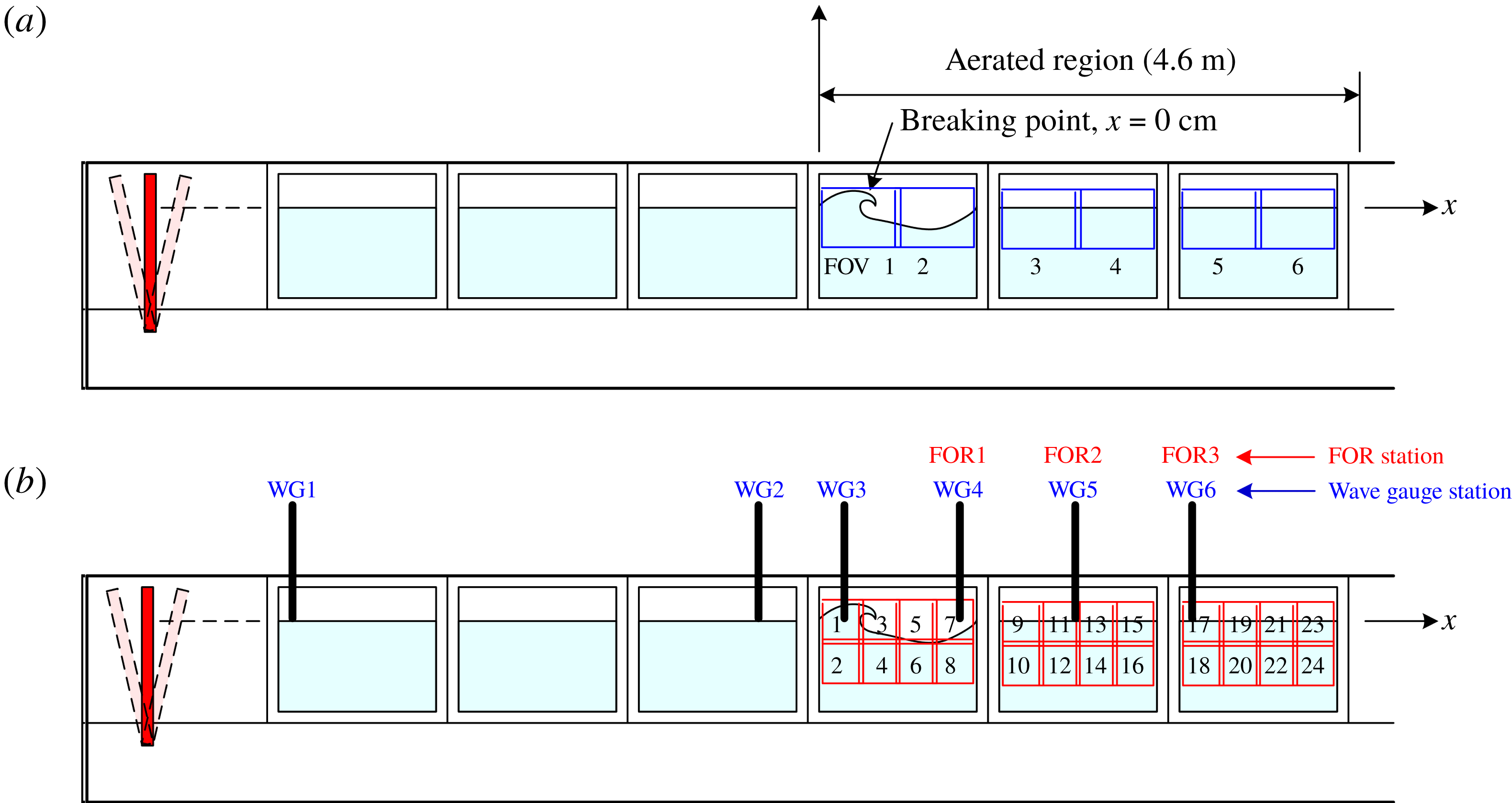
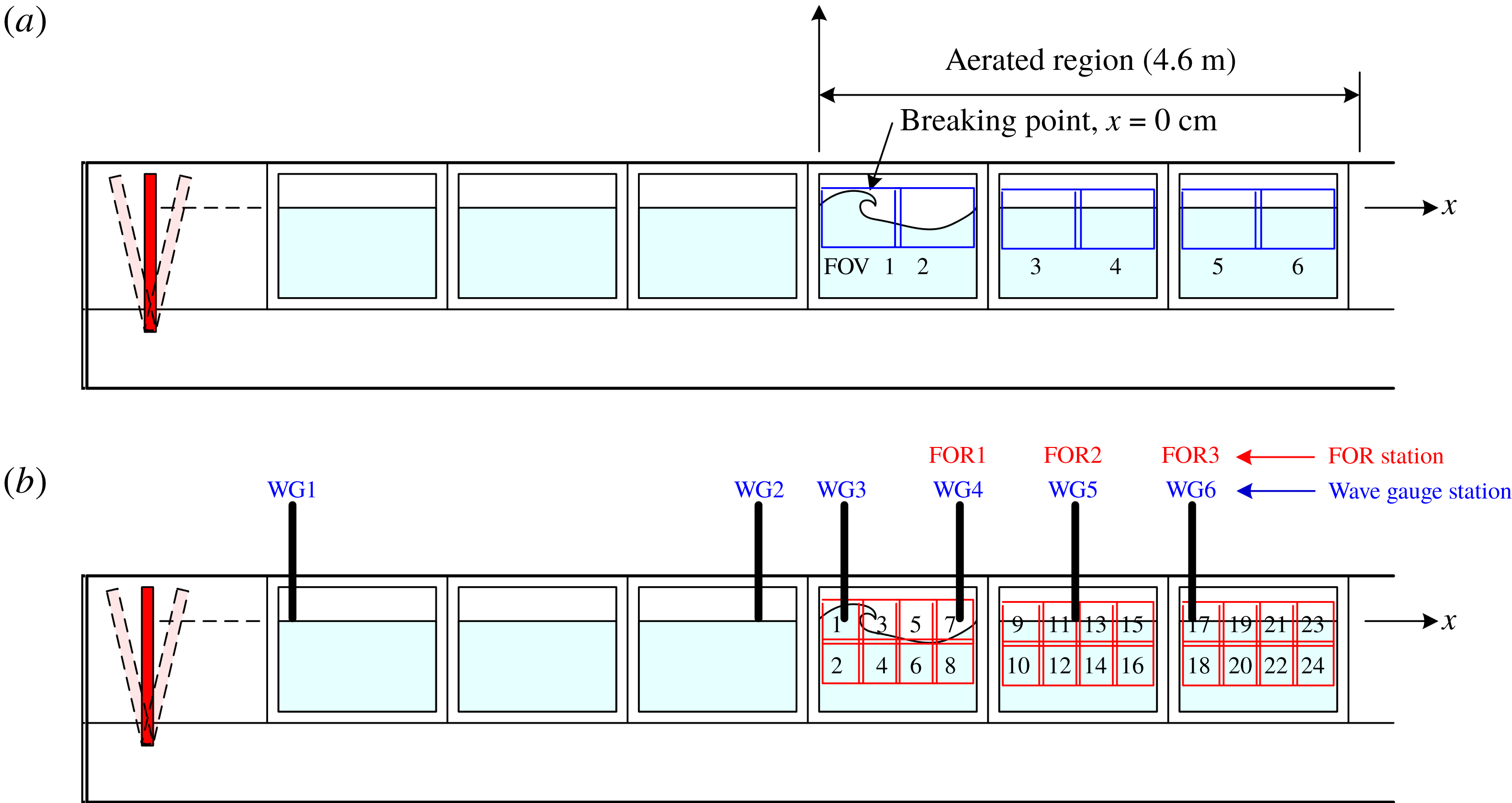
and the specific weight is 1.02. The PIV measurements include 24 fields of view (FOVs) of
 $0.37~\text{m}\times 0.37~\text{m}$
, as shown in figure 1, centred at 0.2 m behind the front tank wall. Note that the bottom is located at
 $z=-0.80~\text{m}$
and the light sheet was redirected upwards by a mirror mounted on the bottom. After acquiring the images, velocities were determined using commercial software from LaVision Inc. The velocity fields were obtained using an adaptive multipass algorithm with an initial interrogation window of
 $64\times 64$
pixels and a final window of
 $32\times 32$
pixels with a 50 % overlap. The spatial resolution of the velocity vectors is
 $16\times 16$
pixels, corresponding to
 $5.78~\text{mm}\times 5.78~\text{mm}$
. There is an overlap of 20 mm between adjacent FOVs. Using the mosaic concepts (Drazen & Melville Reference Drazen and Melville2009; Lim et al.
Reference Lim, Chang, Huang and Na2015), the 24 FOVs cover the entire flow field of the spilling breaker with sufficient spatial and temporal resolutions. Measurements were repeated 20 times at each FOV for subsequent ensemble averaging and turbulence analysis.
Schematic diagram of the wave tank and instrument configuration. The six BIV FOVs are shown in (a), while (b) shows the 24 PIV FOVs.
The BIV technique uses the same bubble–liquid interface tracking algorithm as that in the modified PIV (Ryu, Chang & Lim Reference Ryu, Chang and Lim2005; Ryu, Chang & Mercier Reference Ryu, Chang and Mercier2007; Chang, Ariyarathne & Mercier Reference Chang, Ariyarathne and Mercier2011; Lin et al.
Reference Lin, Hsieh, Lin, Chang and Raikar2012; Lim et al.
Reference Lim, Chang, Huang and Na2015; Na et al.
Reference Na, Chang, Huang and Lim2016). The bubble–liquid interface tracking algorithm has been verified in bubble plumes and hydraulic jumps (Ryu et al.
Reference Ryu, Chang and Lim2005; Ryu & Chang Reference Ryu and Chang2008; Chang et al.
Reference Chang, Ariyarathne and Mercier2011; Lin et al.
Reference Lin, Hsieh, Lin, Chang and Raikar2012). The same camera and framing rate as in the PIV measurements were used in the BIV measurements. Two regular 600 W light bulbs with reflecting mounts and a translucent flat plate were used to illuminate the flow from behind the tank. No lasers are needed in the BIV measurements. The depth of field (DOF) for the captured images is 0.21 m, with its centre at 0.2 m behind the tank’s front wall. The camera was located at 4.7 m in front of the centre of the DOF, resulting in an uncertainty of 2.2 % caused by the limited DOF thickness in the acquired images for later velocity determination. In the BIV measurements, six FOVs of
 $0.66~\text{m}\times 0.50~\text{m}$
were used to cover the entire aerated region of the plunging breaker, as shown in figure 1, resulting in a spatial resolution of
 $0.64~\text{mm}~\text{pixel}^{-1}$
. There is a small overlap region of 84 mm between FOV1 and FOV2, between FOV3 and FOV4, and between FOV5 and FOV6, and a gap of 270 mm between FOV2 and FOV3, and between FOV4 and FOV5 due to a steel column of the wave tank, as shown in figure 1. After acquiring the images, the same software as in PIV was used for velocity determination. An adaptive multipass algorithm with an initial interrogation window of
 $32\times 32$
pixels and a final window of
 $16\times 16$
pixels with a 50 % overlap was applied in the process. Accordingly, the final resolution of the velocity vectors is
 $8\times 8$
pixels, corresponding to
 $5.26~\text{mm}\times 5.26~\text{mm}$
. A time interval,
 $\unicode[STIX]{x0394}t$
, of 2 ms or 4 ms was used for image cross-correlation, depending on the flow velocities. The principle and validation of the BIV technique are detailed in Ryu et al. (Reference Ryu, Chang and Lim2005, Reference Ryu, Chang and Mercier2007), Chang et al. (Reference Chang, Ariyarathne and Mercier2011) and Lin et al. (Reference Lin, Hsieh, Lin, Chang and Raikar2012).
The BIV images were used to qualitatively examine the onset of breaking and bubble plume evolution. Compared to the BIV images, the PIV images are relatively difficult to visualize the bubble plume evolution because the texture of the interface between bubbles and water is not as detailed and pronounced as that in the BIV images. In addition, the PIV field of view is much smaller than that of BIV. Hence the BIV images allow us to see a ‘bigger picture’ of the flow. On the other hand, near the onset of breaking when the aerated region is less prominent, both PIV and BIV images were used for (qualitative) visual examination.
The FOR technique was used to obtain the void fraction in the aerated region of breaking waves. Based on the coherent mixing of scattered signals with Fresnel reflection from the tip of an optical fibre, FOR is capable of measuring the velocity and void fraction of both phases at a given point in the gas–liquid flow. The technique is nearly non-invasive because of its small dimension of the optical fibre (typical diameter
 $125~\unicode[STIX]{x03BC}\text{m}$
), high spatial resolution (typically less than
 $50~\unicode[STIX]{x03BC}\text{m}$
) and high temporal resolution (typically less than
 $10~\unicode[STIX]{x03BC}\text{s}$
). The principle, validation and applications of the FOR technique are described in detail in Chang, Lim & Su (Reference Chang, Lim and Su2002), Chang et al. (Reference Chang, Lim and Su2003), Lim et al. (Reference Lim, Chang, Su and Chen2008) and Ryu & Chang (Reference Ryu and Chang2008). The FOR measurements were sampled at 100 kHz throughout the experiment. There are three FOR measurement stations located at
 $x/L=0.50$
(termed FOR station 1),
 $x/L=1.00$
(FOR station 2) and
 $x/L=1.55$
(FOR station 3), as shown in figure 1. Unlike the plunging breaking wave study in Lim et al. (Reference Lim, Chang, Huang and Na2015), these horizontal locations were chosen somewhat arbitrarily but relative to the wavelength because prominent jet impingement was not easily discernible. The measurement points have a vertical interval of 10 mm while the total number of measurement points at FOR stations 1, 2 and 3 is 10, 10 and eight, respectively. These numbers were determined by the vertical spreading of the bubble cloud, from
 $z=0.04~\text{m}$
to 0.14 m, from 0.02 m to 0.11 m, and from 0.02 to 0.09 m at stations 1, 2 and 3, respectively. Measurements at the location below the lowest point at each station were also performed (not shown here) to verify that the measured void fraction was negligibly small. Measurements were repeated 20 times at each FOR measurement point so mean void fraction could be obtained.
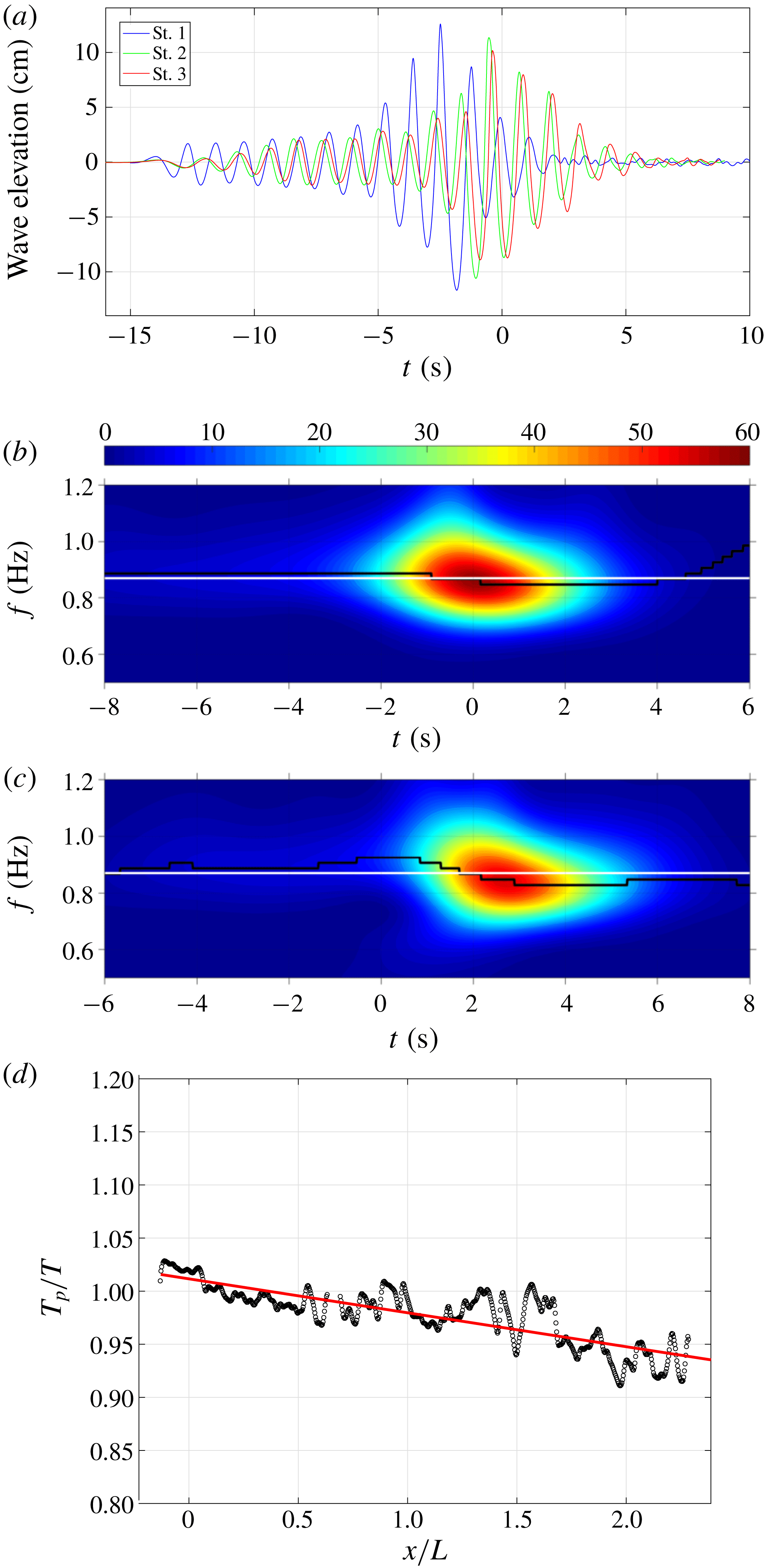
(a) Ensemble-averaged surface elevations measured at WG1 (
 $x/L=-2.53$
), WG2 (
 $x/L=-0.42$
) and WG3 (
 $x/L=-0.06$
) before breaking. (b,c) Wavelet amplitude spectra of the ensemble-averaged surface elevations measured at (b) WG3 and (c) WG6 (FOR station 3 at
 $x/L=1.55$
). In each wavelet amplitude spectrum, the white horizontal line around 0.87 Hz is the central frequency, and the black line is the local peak frequency. (d) Spatial variation of the dimensionless local period with a linear fitting slope of
 $T_{p}/T=1.0-0.03(x/L)$
.
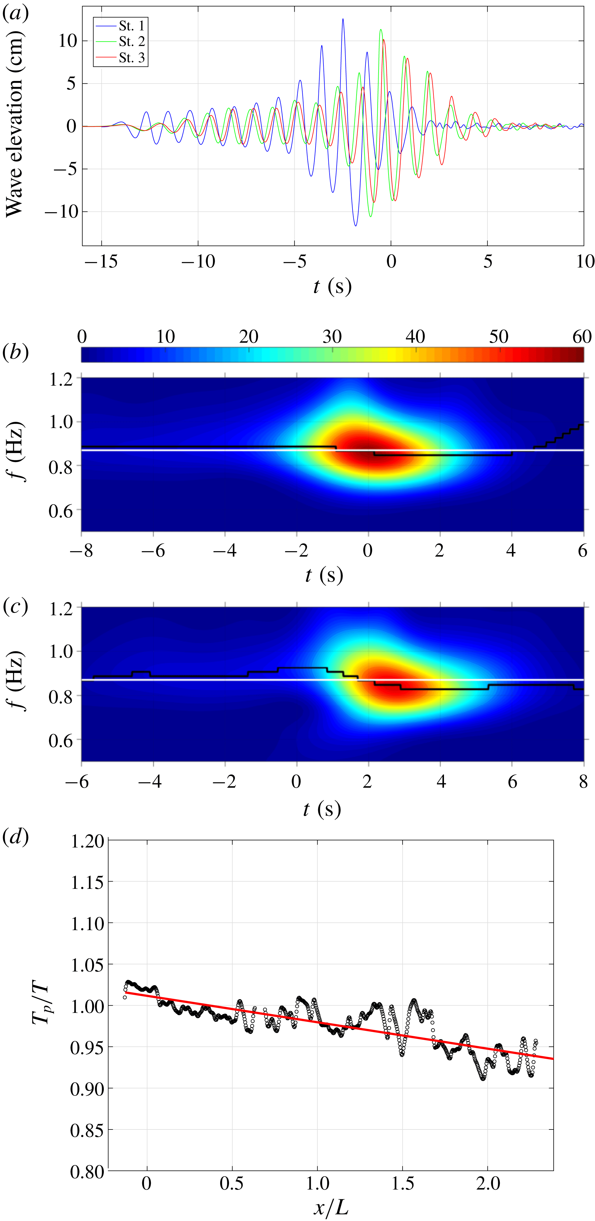
Figure 2(a) shows the measured surface elevations at
 $x/L=-2.53$
(WG1),
 $-0.42$
(WG2) and
 $-0.06$
(WG3) in the pre-breaking region using double-wired resistance-type wave gauges. Surface elevations in the post-breaking region were measured at
 $x/L=0.50$
(WG4), 1.00 (WG5) and 1.55 (WG6), coincident with the FOR stations 1, 2 and 3, respectively. Note that the surface measurements were repeated 20 times so the mean quantities could be obtained. The averaged root-mean-square (r.m.s.) values of the measured surface elevation are
 $\unicode[STIX]{x1D702}_{rms}=0.68{-}0.73~\text{mm}$
for WG1 to WG3 in the pre-breaking region. Since resistance wave gauges measure only the total length in contact with water, the measured surface elevations may be underestimated in the post-breaking region, as shown in Lim et al. (Reference Lim, Chang, Huang and Na2015). The surface profiles for WG3 and WG6 were decomposed into waves with different frequencies and amplitudes based on the wavelet analysis, as shown in figure 2(b,c) in which the contours depict particular frequencies and time instants when the local energy is maximum. The local peak frequency at WG3 is near the central frequency before breaking, and then upshifts to a higher frequency after breaking at WG6. Note that the intensity values of the contours in figure 2(b,c) represent the energy level over the entire breaking process and encompass the entire spatial domain covered by the multiple FOVs in the measurements (i.e. the 24 overlapped FOVs, up to
 $x=2.5L$
) and the entire recording time (up to
 $t\sim 4T$
). Hence, the peak energy level in figure 2(c) does not indicate the energy level of the primary breaking wave because of its significant energy dissipation at WG6.
Figure 2(f) shows the spatial variation of the local wave period downstream from breaking based on PIV images. The local wave period,
 $T_{p}$
, was defined as the time interval between two troughs – the front trough and the rear trough of the progressing breaker. The local wave period is normalized by the wave period of the primary breaking wave,
 $T$
. As shown in figure 2(f),
 $T_{p}/T$
decreases linearly with a slope of
 $-0.03$
as the breaker advances. Tian et al. (Reference Tian, Perlin and Choi2012) reported that the local wavelength
 $L_{p}$
is reduced by 30 % within two wave periods before the onset of spilling breaking. Assuming that the phase speed change is minimal, the wave period must decrease in their study. However, determining the phase speed under breaking waves is ambiguous (Perlin, Choi & Tian Reference Perlin, Choi and Tian2013). Thus Stansell & MacFarlane (Reference Stansell and MacFarlane2002) examined three definitions of the wave phase speed – i.e. phase speed based on (i) linear wave theory, (ii) partial Hilbert transforms of measured surface elevation, and (iii) the local position of maximum surface elevation – and showed great disparity. More recently, Banner et al. (Reference Banner, Barthelemy, Fedele, Allis, Benetazzo, Dias and Peirson2014) found that the phase speed
 $C_{m}$
based on the last definition (horizontal speed of the local maximum surface elevation) decreases near the onset, but then increases immediately after breaking in a spiller based on their simulations (figure 2 in Banner et al.
Reference Banner, Barthelemy, Fedele, Allis, Benetazzo, Dias and Peirson2014). Our measured data confirmed that
 $C_{m}$
is increased by 6 %. So the study is consistent with our measured decrease of
 $T_{p}$
after breaking if
 $C_{m}$
is considered as the correct phase speed. The increase in the phase speed, in turn, causes
 $T_{p}$
to decrease from
 $T_{p}=L_{p}/C_{m}$
.
3 Flow kinematics and turbulence length scale
3.1 Onset of breaking and local wave geometry
Wave breaking is considered as a threshold process, with criteria for predicting breaking onset falling into three categories: geometric, kinematic and energetic (Barthelemy et al.
Reference Barthelemy, Banner, Peirson, Fedele, Allis and Dias2018). The geometric threshold involves wave steepness, wave asymmetry and maximum theoretical steepness, while the kinematic threshold involves horizontal crest particle velocity and the wave phase speed,
 $C$
. The sequential images of breaking onset in Qiao & Duncan (Reference Qiao and Duncan2001), Diorio et al. (Reference Diorio, Liu and Duncan2009) and Duncan et al. (Reference Duncan, Qiao, Philomin and Wenz1999) suggested that the geometrical threshold based on the occurrence of a vertical tangent on the forward face of the crest may not be particularly robust. Nevertheless, examination of kinematic criteria is non-trivial because of the difficulties in determining the horizontal crest particle velocity and the ambiguity in defining
 $C$
for highly unsteady, rapidly evolving breaking crests (Perlin et al.
Reference Perlin, Choi and Tian2013). For the energetic threshold, Barthelemy et al. (Reference Barthelemy, Banner, Peirson, Fedele, Allis and Dias2018) proposed a criterion
 $B_{th}=0.85$
, where
 $B$
is defined as the ratio between the local energy flux and the local energy density projected on the wave propagation direction and
 $B_{th}$
is the threshold value of
 $B$
at which the wave begins to break. At the free surface,
 $B$
effectively is the horizontal velocity at the crest divided by the forward translation speed of the crest (Barthelemy et al.
Reference Barthelemy, Banner, Peirson, Fedele, Allis and Dias2018). Derakhti, Banner & Kirby (Reference Derakhti, Banner and Kirby2018) further suggested that the strength of breaking depends on the rate of change of
 $B$
at the particular moment when
 $B$
is up-crossing the critical value of
 $B_{th}=0.85$
. They numerically obtained the formulation
 $b=0.034(\unicode[STIX]{x1D6E4}-0.30)^{2.5}$
, where
 $b$
is the breaking strength parameter,
 $\unicode[STIX]{x1D6E4}$
is a normalized parameter defined as
 $\unicode[STIX]{x1D6E4}=T_{b}\,\text{d}B/\text{d}t|_{B_{th}}$
and
 $T_{b}$
is the local wave period at breaking.
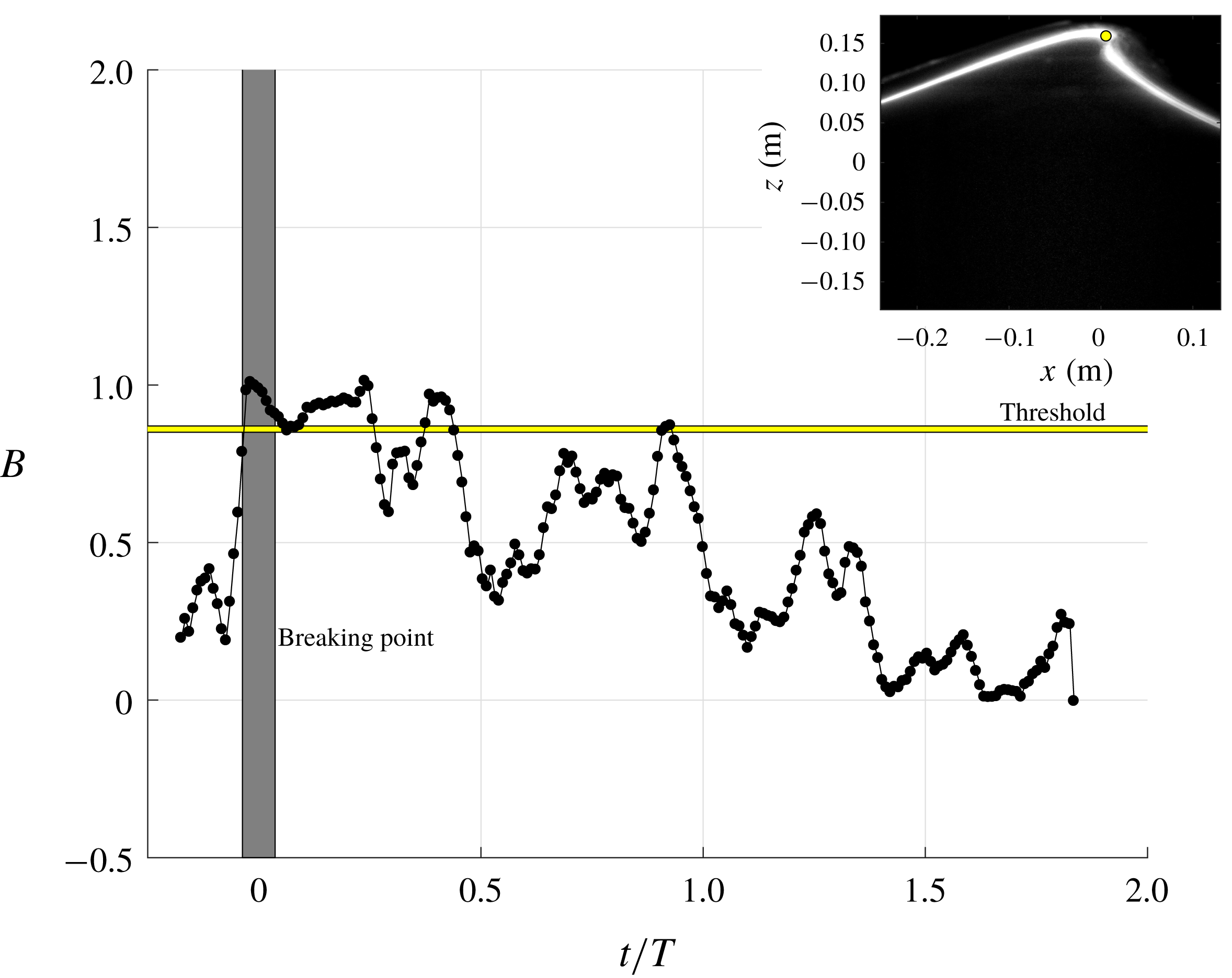
As shown in figure 3, the present experimental data agree with the Barthelemy et al. (Reference Barthelemy, Banner, Peirson, Fedele, Allis and Dias2018) simulations in which
 $B$
sharply increases near the breaking onset. Note that, in the present study,
 $B$
was calculated based on the measured horizontal velocity at the crest peak
 $x_{peak}$
and the phase speed
 $C$
from the linear wave theory. The location of
 $x_{peak}$
was first identified at each time instant from the BIV images. Each data point
 $B$
in figure 3 was then calculated as the horizontal particle velocity at the corresponding location divided by the phase speed
 $C$
. We examined BIV images and videos during those multiple instances when
 $B$
increases after breaking (e.g.
 $t/T\sim 0.3$
, 0.9 and 1.2). Interestingly, the instantaneous BIV images depict that ‘small impinging/splash-up processes’, similar to those in the plunging breakers in Lim et al. (Reference Lim, Chang, Huang and Na2015) but with a much smaller physical scale, occur during this period. So these small impingements and splash-ups could be the possible cause of the multiple threshold crossing of
 $B$
. Banner & Fooks (Reference Banner and Fooks1985) observed disturbances in the free-surface measurements that were caused by the presence of the rearward-travelling shear-layer waves. However, these rearward waves are unlikely to be the cause of the multiple increases of
 $B$
in the present study because the breaking waves used in Banner & Fooks (Reference Banner and Fooks1985) are approximately one order of magnitude smaller in wavelength than those in the present study, and their aeration level is also much lower.
Temporal evolution of
 $B$
at the surface calculated based on the wave propagation direction plotted against the threshold value of
 $B_{th}=0.85$
. The vertical thick grey ‘line’ indicates the range of breaking point. The inset depicts the breaking point, which was geometrically determined from the mean PIV images when a vertical tangent segment appears.

Note that, if
 $C$
is replaced by the forward translation speed of the crest in calculating
 $B$
in figure 3, as stated in Barthelemy et al. (Reference Barthelemy, Banner, Peirson, Fedele, Allis and Dias2018), this speed may be obtained following Saket et al. (Reference Saket, Peirson, Banner, Barthelemy and Allis2017) based on the BIV images. In the present study, the horizontal location of the crest point
 $x_{peak}$
at each time interval of 0.01 s was identified in the BIV images. By linearly fitting the data (the data trend is linear), the averaged crest point speed
 $x_{peak}/t$
was found to be
 $1.06L/T$
or
 $1.06C$
. We prefer the use of
 $C$
instead of
 $x_{peak}/t$
because
 $C$
is readily available. The discrepancy between the averaged crest point speed and
 $C$
is approximately 6 %.
In figure 3, the approximate range of breaking onset (the shaded region) was determined by visual examination of the PIV images when the wave front became vertical. The inset in figure 3 shows the mean PIV image at the breaking onset when a vertical tangent segment appears. As discussed earlier, using visual examination of the wave front becoming vertical to determine the onset of breaking is non-trivial due to the fact that breaking waves are inherently highly irregular and unsteady near the breaking point and deform rapidly after breaking. However, the geometrical criterion used in the present study can be justified by the following reasons: (i) the variation was less than 1 % of the wavelength (and only 5 % of the wave height) among the 20 repeated runs; (ii) the approach does not involve the ambiguity of defining phase speed; and (iii) the approach directly used the measurements in a spatial domain, and thus the ambiguity in transferring a temporal measurement to a spatial measurement is not an issue. We would also like to bring up the difference between spilling breakers used in the present study and the gentle spilling breakers in Qiao & Duncan (Reference Qiao and Duncan2001) and Diorio et al. (Reference Diorio, Liu and Duncan2009) – the present breaking waves are of high intensity (
 $H=0.265~\text{m}$
, high air entrainment with lots of bubbles and a high aeration level due to strong impingement jet-like impact during the process), whereas the breakers in Qiao & Duncan and Diorio et al. (wave heights of the order of
 $H\sim O(0.01~\text{m})$
) are mostly very weak breakers with a very low amount of air entrainment and a very low aeration level. It is relatively easy to identify the vertical tangent line in the present study.
The breaking strength parameter
 $b$
and the normalized parameter
 $\unicode[STIX]{x1D6E4}$
in the present study are 0.012 and 1.09, respectively, which are consistent with the values reported in Derakhti et al. (Reference Derakhti, Banner and Kirby2018). Noticeably, in the present study, multiple increases of
 $B$
exceeding 0.85 were observed. Through examining the corresponding BIV images, the occurrences of very weak impingements of the overturning jets (of a single breaking wave as it propagated) were coincident with those multiple exceedances. This may suggest that multiple weak jet impingements occurred in the spilling breaker and these impingements caused
 $B$
to increase. Interestingly, the rate of change of
 $B$
for those increases is very similar, implying that the strength of breaking (i.e. impingements of the jets) may also be similar. We also observed that
 $B$
exceeds 0.85 near the breaking point under plunging breaking waves (not shown) using the data from Lim et al. (Reference Lim, Chang, Huang and Na2015). Therefore, the breaking criterion was applied to both spilling and plunging breakers.
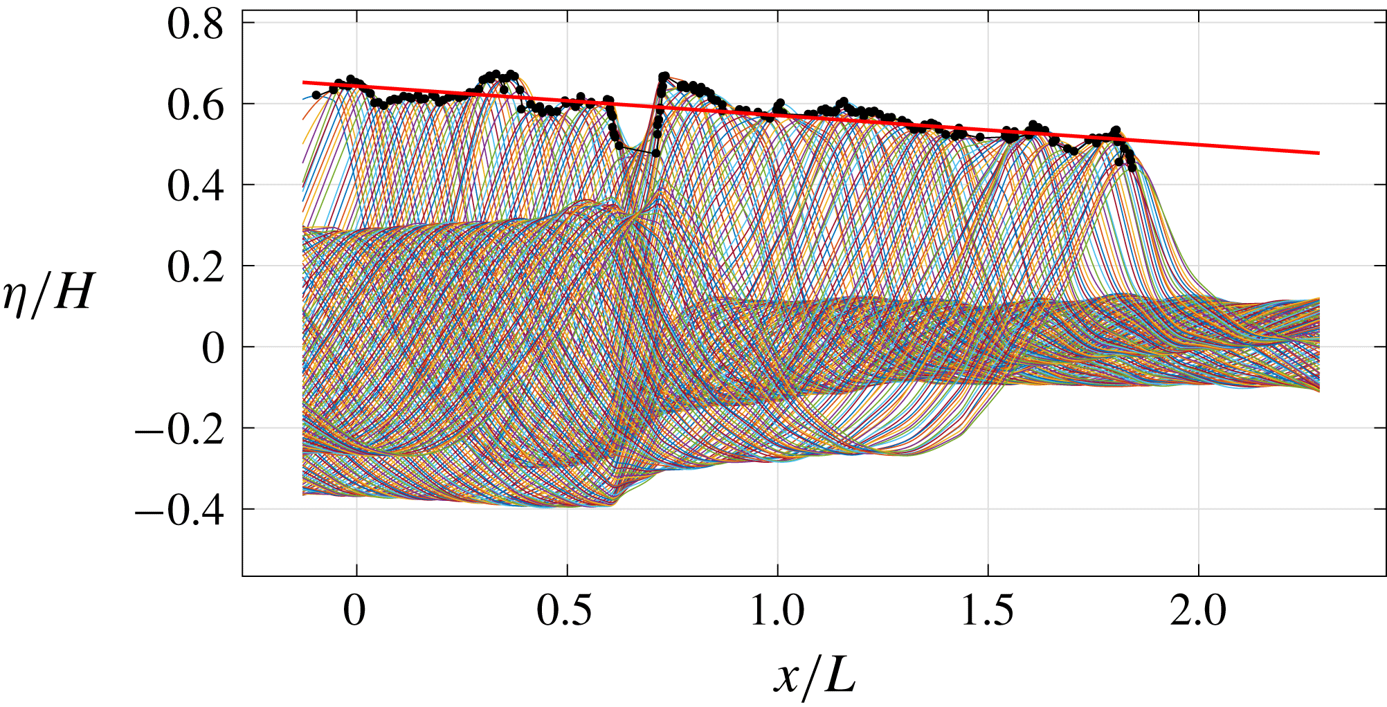
Figure 4 shows the trajectory of the dimensionless breaking wave crest. As shown by the linear least-squares fit, the crest height decreased continuously with a constant slope of
 $-0.08$
over the entire breaking process. Through laboratory experiment, Tian et al. (Reference Tian, Perlin and Choi2012) showed that the crest height of spilling waves is more uniform compared to that of plunging waves. They related the difference in the growth/decay rate of the crest height to the breaking strength parameter,
 $b$
. That is in agreement with Diorio et al. (Reference Diorio, Liu and Duncan2009), while the reason for spillers to have a lower growth rate is their weaker breaking strength. Furthermore, Tian et al. (Reference Tian, Perlin and Choi2012) observed that the crest height of plungers decreases rapidly following the wave breaking, corresponding to a significant loss of potential energy. However, no abrupt decrease of the crest height was observed for the spillers.
Spatial variation of the dimensionless crest profiles and trajectory. The crest profiles were identified using the BIV images while the solid circles indicate the local maxima. The solid line is the linear least-squares fit of the local maxima with a slope of
 $-0.08$
.

3.2 Flow kinematics, vorticity and turbulence
The instantaneous velocity fields measured using PIV were ensemble-averaged to obtain the mean velocity fields
 $(U,W)$
from 20 repeated runs, i.e.
 $$\begin{eqnarray}\displaystyle & \displaystyle U(x,z,t)=\frac{1}{N}\mathop{\sum }_{i=1}^{N}u_{i}(x,z,t), & \displaystyle\end{eqnarray}$$
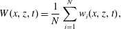 $$\begin{eqnarray}\displaystyle & \displaystyle W(x,z,t)=\frac{1}{N}\mathop{\sum }_{i=1}^{N}w_{i}(x,z,t), & \displaystyle\end{eqnarray}$$
where
 $u_{i}$
and
 $w_{i}$
are the instantaneous horizontal and vertical velocities, the subscript
 $i$
represents the
 $i$
th measurement, and
 $N$
is the total number of repeated runs (
 $N=20$
in the present study). The averaged r.m.s. velocity fluctuations are
 $u_{rms}=0.016~\text{m}~\text{s}^{-1}$
and
 $w_{rms}=0.011~\text{m}~\text{s}^{-1}$
before breaking.
To ensure that the instantaneous velocity field is based on the air bubbles in the measurement plane, we limited the DOF and shortened the exposure time by carefully setting up the camera and lens. By limiting the DOF, the objects located in front of the DOF near the front wall appear to be blurred due to being out of focus. The image intensity of the bubbles in these blurred images is significantly weaker than those in the sharp, focused images, so they have little effect on the correlation process (i.e. much lower image intensity/peak and therefore much lower correlation peak in PIV analysis). Figure 5 in Ryu et al. (Reference Ryu, Chang and Lim2005) showed that the velocity measured from the correlation of the superimposed sharp and blurry images is very close to the velocity measured from the sharp images alone. Moreover, by shortening the exposure time as well as using a weak continuous laser, we minimized image saturation for bubbles illuminated by the laser inside the light sheet, thus providing insignificant light intensity (and thus insignificant correlation contribution) to the bubbles near the front wall outside the light sheet.
Mean relative velocity fields (
 $U-C$
,
 $W$
), with only one-quarter of the velocity vectors plotted, superimposed on mean images for (a)
 $t/T=-0.01$
(FOV1), (b) 0.13 (FOV3), (c) 0.28 (FOV5), (d) 0.40 (FOV7), (e) 0.67 (FOV9), (f) 0.84 (FOV11), (g) 0.99 (FOV13), (h) 1.17 (FOV15), (i) 1.40 (FOV17), (j) 1.66 (FOV19), (k) 1.91 (FOV21) and (l) 2.14 (FOV23). The yellow dots represent the locations of the local maximum horizontal velocity. (m) Temporal variation of the maximum horizontal velocity.
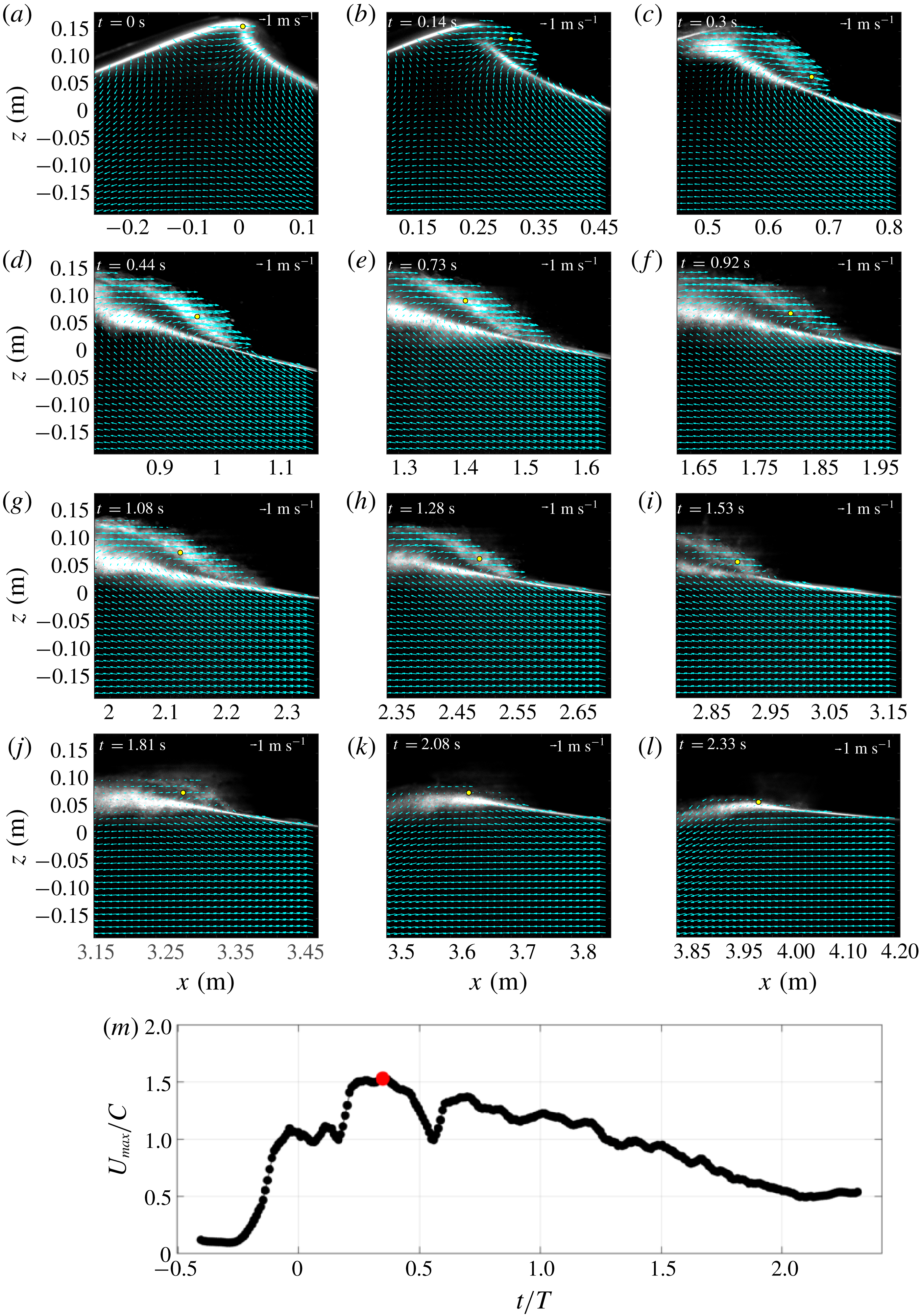
Figure 5 shows the measured mean relative velocity fields
 $(U-C,W)$
with one-quarter of the velocity vectors plotted (every other row and every other column). Note that the velocities were plotted on a moving frame (moving with
 $C$
) so the vortical motion inside the aerated region is legible, and the free surface was identified based on high contrasts between the bright bubble cloud region and the dark air region above in the PIV images. The breaking onset was initiated without an explicit jet impinging onto the quiescent front. When the primary breaking wave front becomes vertical, the maximum horizontal velocity reaches
 $1.1C$
at this breaking point (figure 5
a,m). The same value was found in Duncan (Reference Duncan2001) under weak spilling breaking waves. In plunging breaking waves, higher values of
 $1.3C$
(Perlin, He & Bernal Reference Perlin, He and Bernal1996) and
 $1.4C$
(Lim et al.
Reference Lim, Chang, Huang and Na2015) were reported at the breaking point. Spilling waves may be initiated from the bumpy surface or small jet impingement (Duncan Reference Duncan2001). It is difficult to confirm which of the two processes led to breaking based on figure 5(a–c) and the corresponding BIV images (not shown here). However, it is clear from the images that a small aerated region is formed after the wave passes the breaking point and that this region grows as the wave propagates, similar to what was reported in Duncan et al. (Reference Duncan, Philomin, Qiao and Kimmel1994) and Rojas & Loewen (Reference Rojas and Loewen2010). As the breaking progresses, the vertical location of the maximum horizontal velocity shifts lower (figure 5
a–c), and a shear zone between the high-velocity aerated region and the low-velocity non-aerated region persists, developing turbulence near the lower boundary of the aerated region. At the later stages of breaking (figure 5
e,f), the maximum velocities are found to locate near the middle of the bubble plume as the wave propagates. The magnitude of the maximum horizontal velocity during the entire breaking process is
 $1.5C$
, found near the shear zone at
 $t/T=0.35$
(figure 5
m) occurring in between figures 5(c) and 5(d).
Note that the darker, blurred region dividing the upper and lower foamy (white) regions in figure 5(d–i) is caused by the bubbly flow between the front wall of the wave flume and the light sheet plane (i.e. out-of-focus bubbles near the front wall). These bubbles close to the front wall may block a certain area in the image. Nevertheless, the camera used in the current study has a high light sensitivity and a high dynamic range. With the carefully controlled laser power and camera exposure time, the camera was able to capture even the low-light-intensity tracers within these blurred regions except for the infrequent cases when the entire PIV interrogation window was completely blocked by the bubbles. Note that the original images are much darker in those bright areas but enhanced in the plot for better visualization and identification of the aerated region and boundaries. The instantaneous PIV velocities (not shown here) in the present spilling breakers are similar to those in the plunging breakers reported in Lim et al. (Reference Lim, Chang, Huang and Na2015). It is noted that the number of empty velocity vectors is relatively low even in the highly aerated region.
The instantaneous horizontal and vertical fluctuating velocities,
 $u^{\prime }$
and
 $w^{\prime }$
, are computed as
 $$\begin{eqnarray}\displaystyle & \displaystyle u^{\prime }(x,z,t)=u(x,z,t)-U(x,z,t), & \displaystyle\end{eqnarray}$$
 $$\begin{eqnarray}\displaystyle & \displaystyle w^{\prime }(x,z,t)=w(x,z,t)-W(x,z,t). & \displaystyle\end{eqnarray}$$
Since the cross-tank velocity component was not measured, we define a two-dimensional turbulent intensity
 $I_{2D}$
as
 $$\begin{eqnarray}I_{2D}=\sqrt{\langle u^{\prime \,2}\rangle +\langle w^{\prime \,2}\rangle },\quad I_{x}=\sqrt{\langle u^{\prime \,2}\rangle },\quad I_{z}=\sqrt{\langle w^{\prime \,2}\rangle },\end{eqnarray}$$
where
 $\langle ~\rangle$
denotes the ensemble-average operator. The estimated uncertainty for turbulent intensity using bootstrapping is
 $0.018~\text{m}~\text{s}^{-1}$
, equivalent to
 $0.011C$
.
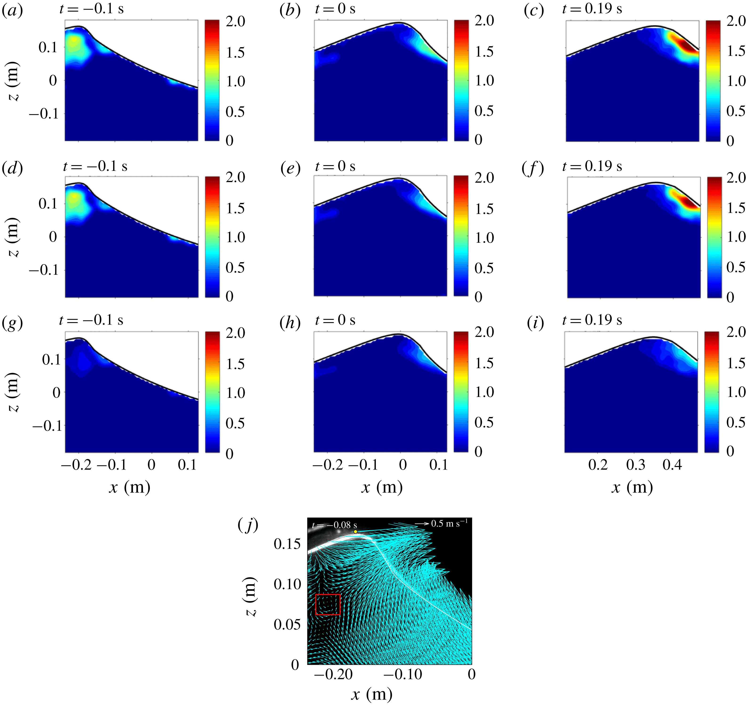
Turbulent intensity fields (
 $\text{m}~\text{s}^{-1}$
) near the onset of breaking at (a,d,g)
 $t/T=-0.09$
, (b,e,h) 0 and (c,f,i) 0.17. (a–c) Turbulent intensity
 $I_{2D}$
; (d–f) horizontal turbulent intensity
 $I_{x}$
; and (g–i) vertical turbulent intensity
 $I_{z}$
. (j) Mean velocity field (
 $U-C,W$
) at
 $t/T=-0.07$
. The estimated uncertainty for turbulent intensity using bootstrapping is
 $0.018~\text{m}~\text{s}^{-1}$
, equivalent to
 $0.011C$
.

Figure 6 shows the turbulent intensity fields near the onset of breaking. Before the wave front becomes vertical, turbulence has already appeared in the middle of the crest (figure 6 a,d). The onset of breaking in the present study was determined from the images by manually identifying the moment when the wave front becomes vertical. This is related to the kinematic breaking criteria, which often involve the horizontal crest particle velocity and the wave phase speed (Perlin et al. Reference Perlin, Choi and Tian2013). Perlin et al. (Reference Perlin, He and Bernal1996) and Chang & Liu (Reference Chang and Liu1998) supported these criteria by experimentally confirming that the horizontal crest particle velocity exceeds the wave phase speed when the wave becomes vertical. Nevertheless, determining the horizontal crest particle velocity is difficult, and defining the phase speed is somewhat ambiguous (Perlin et al. Reference Perlin, Choi and Tian2013). Hence, the onset of breaking may have occurred earlier and caused the turbulence in the middle of the crest (probably transferred from the front face of the crest). By examining the mean velocity before breaking, we observed the presence of a weak roller as depicted in figure 6(j). Although the cause is not clear, this roller may be a possible indication of turbulence in the middle of the crest. The horizontal turbulent intensity is more dominant in the inner region of the crest when compared to the vertical turbulent intensity, as shown in figure 6(d,g). A thin layer of turbulence formed following the wave front is initiated at the beginning of the process (figure 6 a,d,g). This thin layer of turbulence may be generated from the thin shear layer created by the initial impact of the jet (Tulin Reference Tulin, Grue, Gjevik and Weber1996). Nevertheless, we do not believe that this is similar to the jet impingement mechanism in plunging breakers. As the breaking wave progresses, the thin layer of turbulence becomes thicker and increases in intensity. Longuet-Higgins & Turner (Reference Longuet-Higgins and Turner1974) theoretically modelled spilling breakers, predicting that this layer of turbulence moves downslope with a constant acceleration, and its thickness increases linearly with distance from the crest. Similarly, Kimmoun & Branger (Reference Kimmoun and Branger2007) observed that spilling breakers are initiated from a small region of bubbles on the forward side of the crest; the region then becomes turbulent and grows by spreading downslope. Figure 6 and the corresponding BIV images (not shown) qualitatively show the bubble plume evolution.
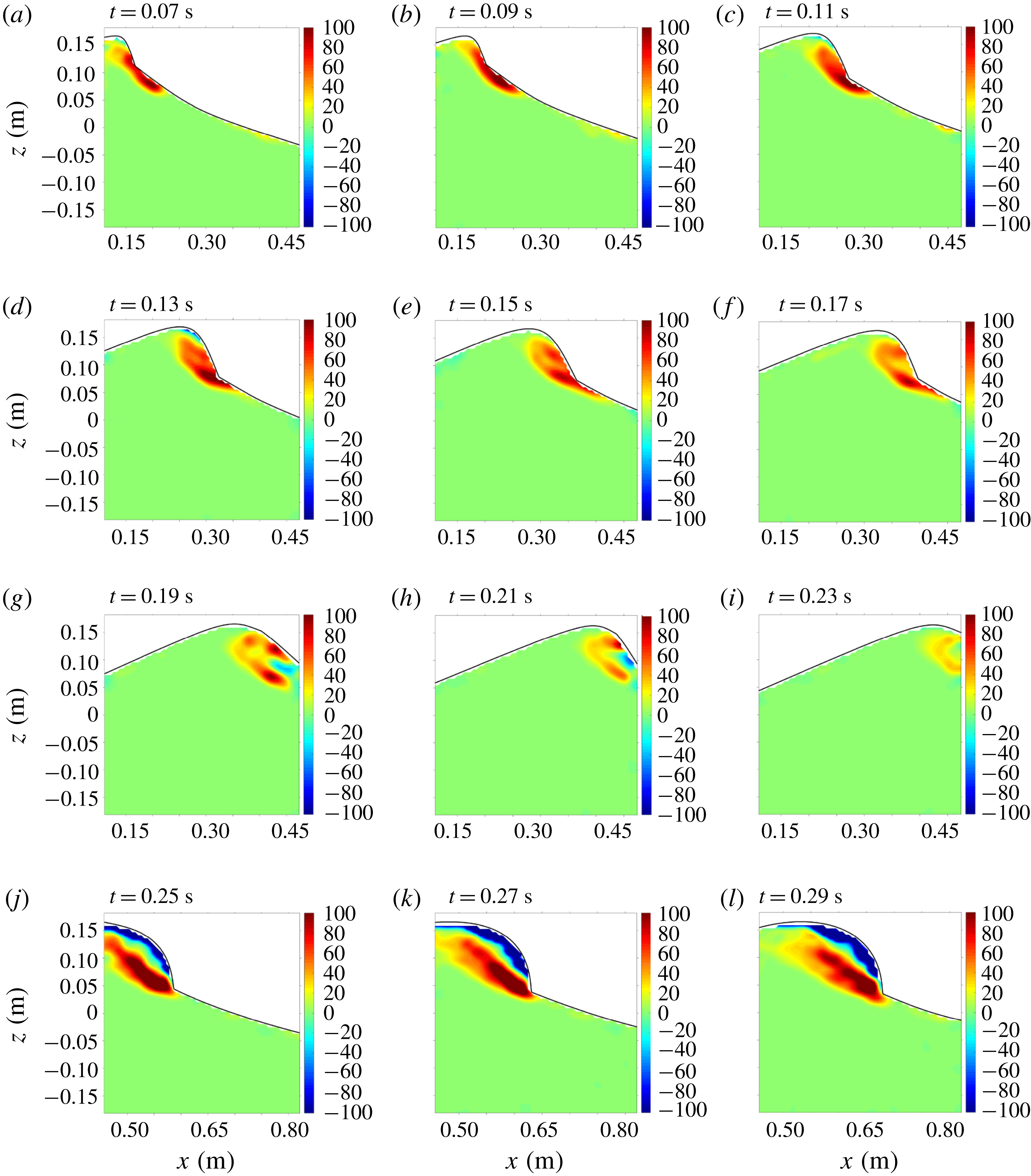
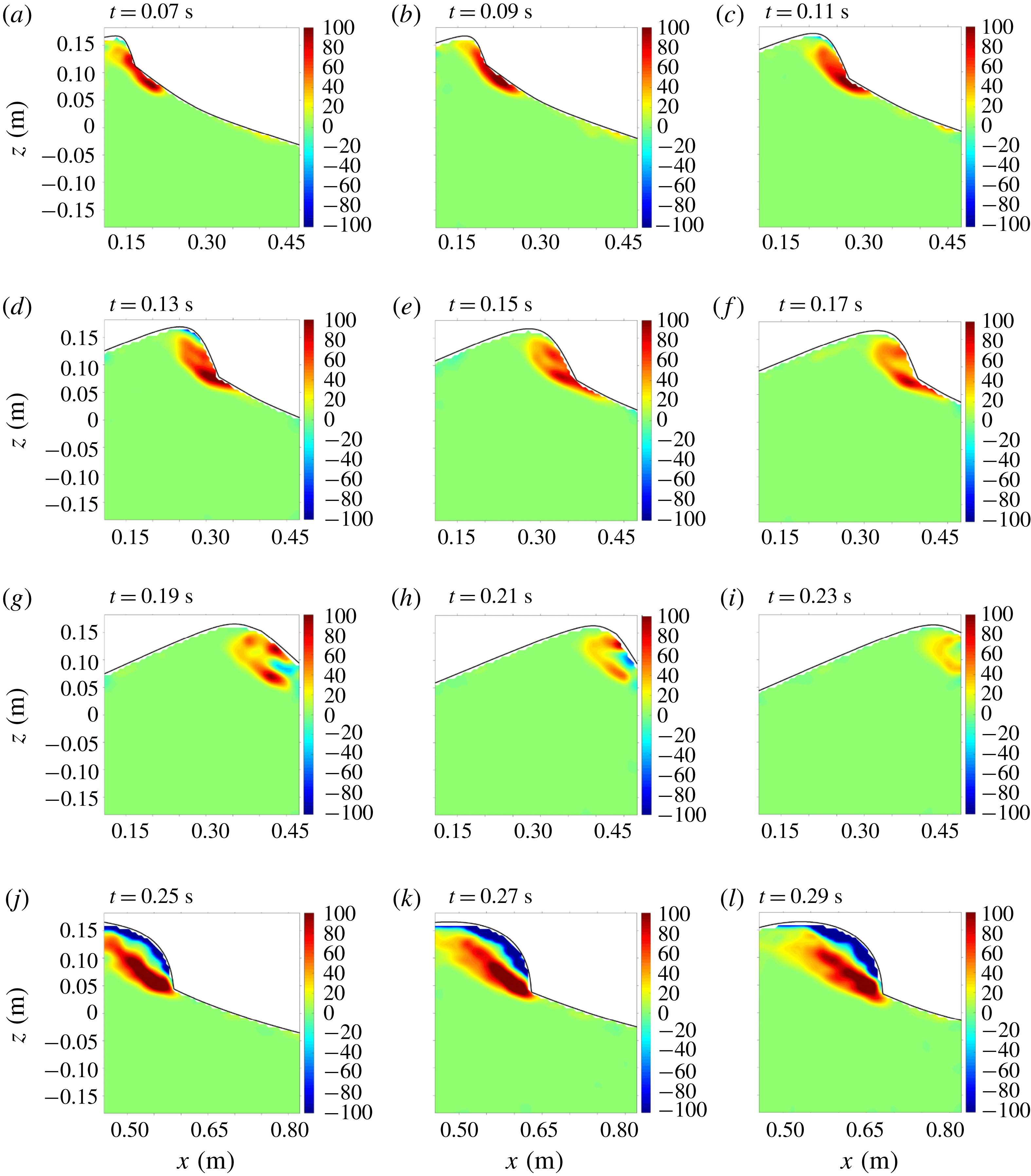
Figure 7 shows the mean vorticity fields. As shown in the figure, a vortical region spreads along the surface located mainly below the toe immediately after breaking. As the breaking progresses, the vortical region stretches and extends to the crest above the toe (figure 7
f). Subsequently, negative vorticity appears near the toe, then moves downward along the wave front (figure 7
i) and fills the upper crest region above the shear zone between the fast-moving aerated region and the quiescent region below (figure 7
l). These processes are in agreement with the finding of Duncan et al. (Reference Duncan, Qiao, Philomin and Wenz1999) and Duncan (Reference Duncan2001). However, Duncan (Reference Duncan2001) extensively discussed the development of the ripples which are not discernible from the present BIV images. The ripples are not likely to be observed in the present study because the breaking wave has a wavelength of
 $L=1.84~\text{m}$
that is much longer than
 $0.77~\text{m}\leqslant L\leqslant 1.18~\text{m}$
generated in Duncan et al. (Reference Duncan, Qiao, Philomin and Wenz1999). Relatively longer-wavelength spillers, such as those in the present study, have weaker dependence on the surface tension forces. As a result, bubbles and spray associated with the intense splashing motions are produced (Duncan Reference Duncan2001), and the effects of the bubbles and spray on the flow become significant.
Mean vorticity fields (
 $\text{s}^{-1}$
) at (a)
 $t/T=0.06$
, (b) 0.08, (c) 0.10, (d) 0.12, (e) 0.14, (f) 0.16, (g) 0.17, (h) 0.19, (i) 0.21, (j) 0.23, (k) 0.25 and (l) 0.27. The estimated uncertainty for vorticity using bootstrapping is
 $0.30~\text{s}^{-1}$
, equivalent to
 $0.05C/H$
.
3.3 Wavelet-educed turbulence length scale
Whether a breaking wave has sufficient turbulent kinetic energy to overcome the stabilizing effects of gravity and surface tension depends on the characteristic turbulent length scale (Brocchini & Peregrine Reference Brocchini and Peregrine2001). If turbulent kinetic energy exceeds the stabilizing energy due to gravity and surface tension, the surface breaks up into bubbles and droplets. In the present study, we used a wavelet-based method to compute the turbulent length scale under the spilling breakers.
Coherent structures can be educed using a wavelet transform with the Morlet mother wavelet defined as
 $$\begin{eqnarray}\unicode[STIX]{x1D711}(z)=\text{e}^{iw_{0}z}\text{e}^{-z^{2}/2},\end{eqnarray}$$
where
 $z$
is the position of the signal for the (different) window of the mother wavelet, and
 $w_{0}=6$
is suggested to satisfy the admissibility condition (Farge Reference Farge1992). The wavelet coefficient of a velocity signal is then defined as the following using the continuous wavelet transform (Farge Reference Farge1992):
 $$\begin{eqnarray}W_{f}(s,z)=\frac{1}{\sqrt{s}}\int _{-\infty }^{\infty }u(\unicode[STIX]{x1D70F})\unicode[STIX]{x1D711}^{\ast }\left(\frac{\unicode[STIX]{x1D70F}-z}{s}\right)\,\text{d}\unicode[STIX]{x1D70F},\end{eqnarray}$$
where
 $u(\unicode[STIX]{x1D70F})$
is the horizontal velocity,
 $s$
is the scale dilation parameter,
 $\unicode[STIX]{x1D70F}$
is the translation parameter,
 $\sqrt{s}$
is for energy normalization across the different scales,
 $^{\ast }$
denotes the complex conjugate, and the integrand represents a convolution product between the dilated and the translated counterpart of the complex conjugate of the mother wavelet. A quantitative local intermittency measure
 $(LIM)$
introduced by Farge (Reference Farge1992) is defined as follows:
 $$\begin{eqnarray}LIM(s,z)=\frac{[W_{f}(s,z)]^{2}}{\langle [W_{f}(s,z)]^{2}\rangle _{z}},\end{eqnarray}$$
where
 $\langle [W_{f}(s,z)]^{2}\rangle _{z}$
is the average of the squared wavelet coefficient along the
 $z$
direction. The
 $LIM$
peak among different scales can be formulated as
 $$\begin{eqnarray}LIMM(z)=\max \{LIM(s,z)\}.\end{eqnarray}$$
The value of
 $LIMM$
represents the energy level of the most excited mode among the scale bands. Camussi & Felice (Reference Camussi and Felice2006) reported that inverting the scale dilation parameter of
 $LIMM$
directly gives the length scale (
 $LS$
) of the identified vortex. Following Na et al. (Reference Na, Chang, Huang and Lim2016), we used a conditional threshold,
 $LIM=0.01$
, assigned to the columns with
 $\langle [W_{f}(s,z)]^{2}\rangle _{z}<0.01$
, to separate the laminar flow region in which the
 $LIM$
approach is not applicable. Na et al. (Reference Na, Chang, Huang and Lim2016) reports that
 $LS$
not only represents the length scale of the most energetic eddies, but also is comparable to the integral length scale. In the present study, the obtained instantaneous
 $LIMM$
and
 $LS$
are ensemble-averaged to obtain the mean
 $LIMM$
and
 $LS$
.
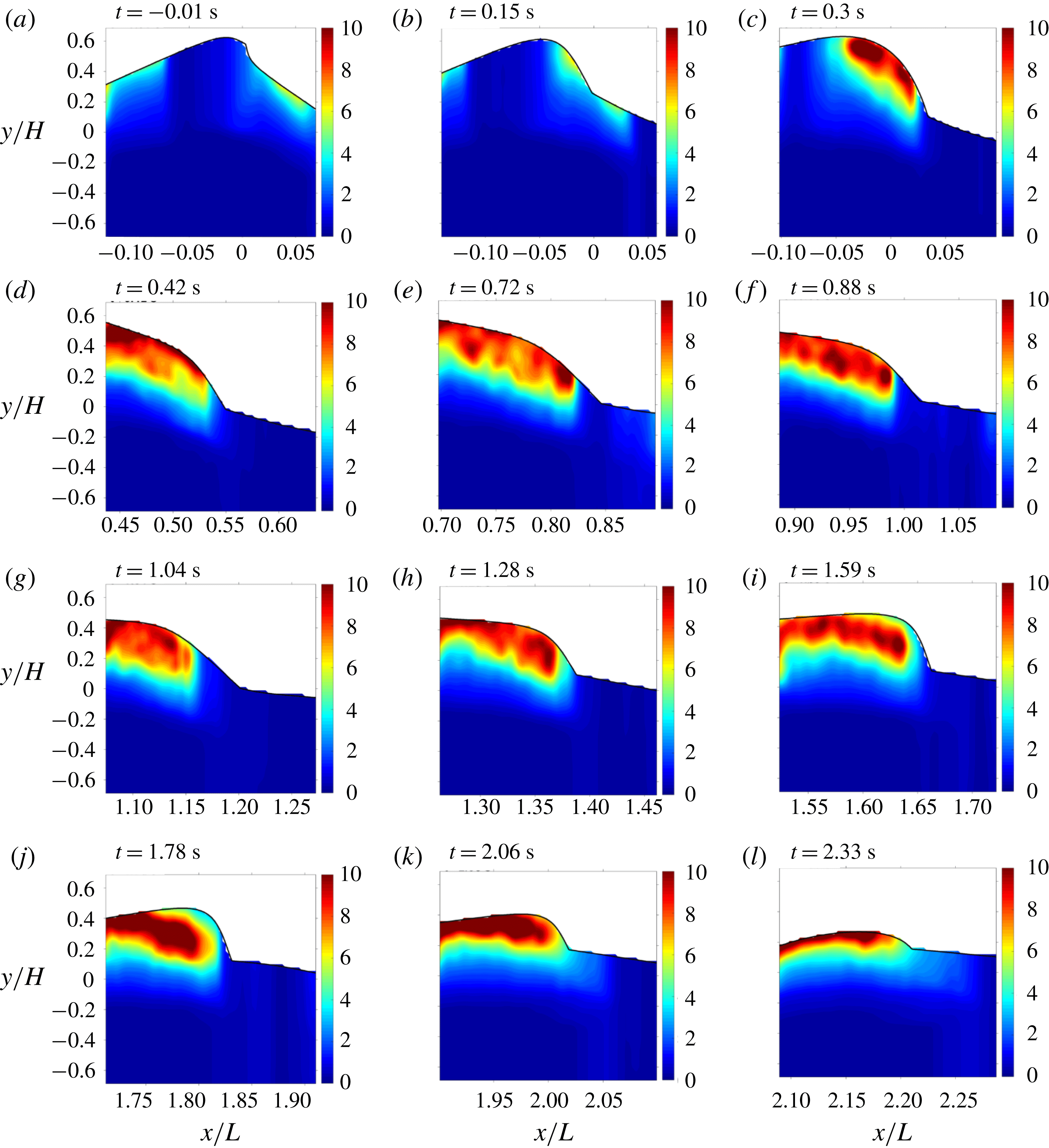
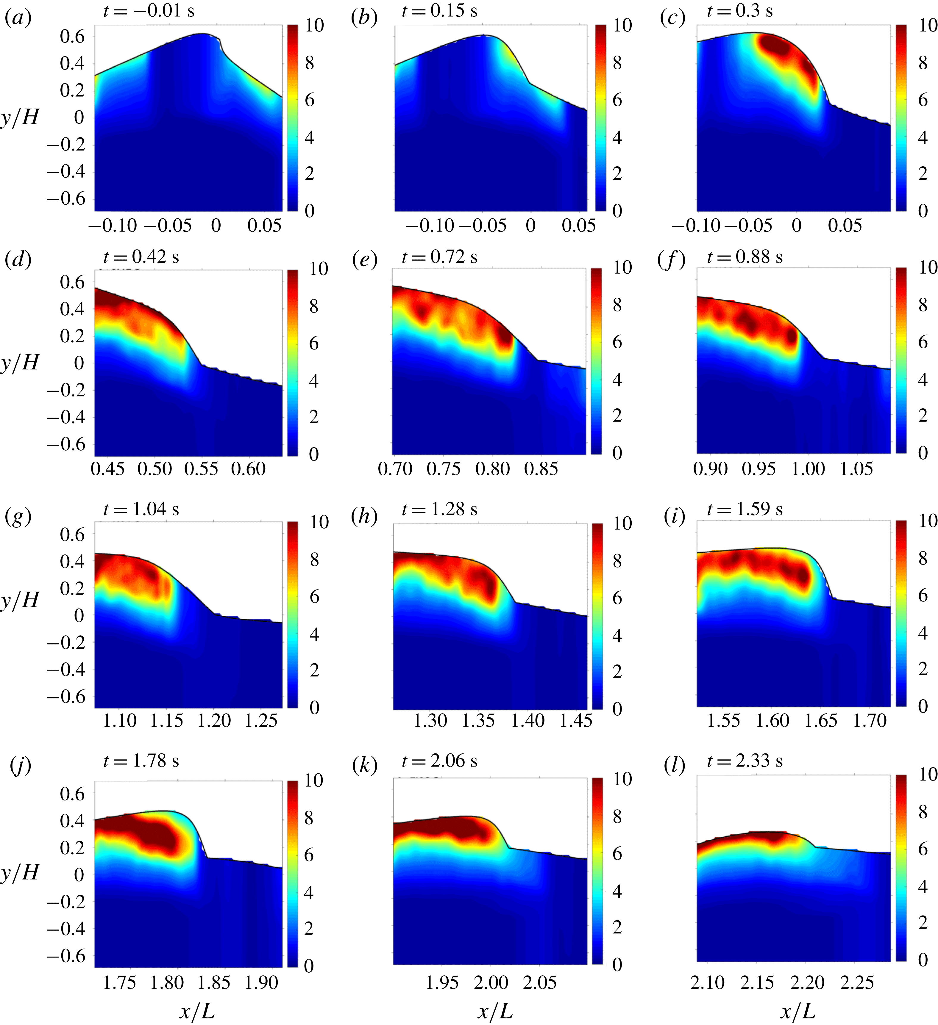
In figure 8, the ensemble-averaged length scale
 $LS$
, normalized by the wave height
 $H$
, is presented. The
 $H/LS$
plots were selected such that the wave front approximately locates at the middle of each FOV. The normalized length scale of eddies inside the aerated region ranges between
 $H/LS=5$
and 12 (i.e. length scale
 $LS=2{-}5~\text{cm}$
) during the entire breaking processes. The length scale increases near the lower boundary of the aerated region. Govender et al. (Reference Govender, Mocke and Alport2004) showed that the length scale increases downwards from crest to trough, ranging from approximately
 $LS=0.1h$
to
 $0.4h$
(approximately
 $0.1h$
at the crest) under surf-zone spillers. This length scale is similar to the value found in the present results (approximately
 $0.07h$
at the crest). Previous studies (e.g. Govender et al.
Reference Govender, Mocke and Alport2004; Longo Reference Longo2009; Huang et al.
Reference Huang, Hwung and Chang2010) reported that the turbulence length scales are less than the wave height. The normalized turbulent length scales are in the range of
 $LS/H=0.05$
to 0.3 in Govender et al. and Huang, and
 $LS/H=0.02$
to 1.0 in Longo. Note that the laboratory spilling breaker heights vary from
 $H=3$
to 16 cm among these three studies. In the present study featuring a much greater wave height of
 $H=26.5~\text{cm}$
, the turbulence length scale is in the range of
 $LS/H=0.08{-}0.2$
under the spillers, comparable to the reported length scales above.
Normalized length scale (
 $H/LS$
) at (a)
 $t/T=-0.01$
(FOV1), (b) 0.14 (FOV3), (c) 0.28 (FOV5), (d) 0.39 (FOV7), (e) 0.66 (FOV9), (f) 0.81 (FOV11), (g) 0.95 (FOV13), (h) 1.17 (FOV15), (i) 1.46 (FOV17), (j) 1.63 (FOV19), (k) 1.89 (FOV21) and (l) 2.14 (FOV23).
When compared to the values of
 $H/LS=7{-}20$
in the highly aerated region of plunging breakers in Na et al. (Reference Na, Chang, Huang and Lim2016), the
 $LS$
values are comparable but confined to a narrower range in the present spilling breakers. Interestingly, figure 8(a) depicts that
 $H/LS$
just downstream of the toe increases to
 $H/LS=4{-}7$
near the onset of breaking. Duncan (Reference Duncan2001) discussed that for long-wavelength spilling breakers, like the ones in the current study, the spilling process starts with the appearance of a rough surface, which probably causes the increased turbulent length scales on the forward face of the crest. In the present study, the
 $LS$
value stays less than
 $0.2H$
above the shear zone between the fast-moving aerated region and the quiescent water region below (figure 8
b–j). By examining figures 5 and 8, one can see that the region above the lower boundary of the white foamy region exhibits a characteristic length scale of approximately
 $LS/H\sim 0.1{-}0.2$
(with some variations inside) in figure 8. However, in figure 8 the length scale immediately to the left of the toe is almost one order of magnitude greater
 $(LS/H\sim 1{-}2)$
. We used a conditional threshold,
 $LIM=0.01$
, assigned to the columns with
 $\langle [W_{f}(s,z)]^{2}\rangle _{z}<0.01$
, to separate the laminar flow region in which the
 $LIM$
approach is not applicable. The abrupt change of the length scale near the toe is due to
 $\langle [W_{f}(s,z)]^{2}\rangle _{z}$
being barely below 0.01 at this location. The discrete jump in the conditional threshold approach forces this abrupt and unrealistic change.
4 Effects of void fraction
4.1 Void fraction and its effects on flow structures
The FOR technique was used to resolve phases (air and water in this study) with a high temporal resolution. With 20 repeated instantaneous void fraction (
 $\unicode[STIX]{x1D6FC}$
) measurements at each measurement point, the mean void fraction is computed by ensemble averaging, i.e.
 $$\begin{eqnarray}\langle \unicode[STIX]{x1D6FC}(x,z,t)\rangle =\frac{1}{N}\mathop{\sum }_{i=1}^{N}\unicode[STIX]{x1D6FC}_{i}(x,z,t),\end{eqnarray}$$
where
 $\langle \unicode[STIX]{x1D6FC}(x,z,t)\rangle$
is the mean void fraction,
 $\unicode[STIX]{x1D6FC}_{i}$
is the
 $i$
th local instantaneous void fraction and
 $N=20$
is the number of repeat runs in the experiment. To match the temporal resolution of the PIV velocity measurements, the original sampling rate of 100 kHz was averaged over every 1000 points, resulting in a final rate of 100 Hz for
 $\langle \unicode[STIX]{x1D6FC}\rangle$
. Furthermore, the wave-averaged (wet-period-averaged) void fraction
 $\unicode[STIX]{x1D6FC}_{wa}$
is defined as
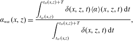 $$\begin{eqnarray}\unicode[STIX]{x1D6FC}_{wa}(x,z)=\frac{\displaystyle \int _{t_{tr}(x,z)}^{t_{tr}(x,z)+T}\unicode[STIX]{x1D6FF}(x,z,t)\langle \unicode[STIX]{x1D6FC}\rangle (x,z,t)\,\text{d}t}{\displaystyle \int _{t_{tr}(x,z)}^{t_{tr}(x,z)+T}\unicode[STIX]{x1D6FF}(x,z,t)\,\text{d}t},\end{eqnarray}$$
where
 $t_{tr}(x,z)$
is the time when the front trough reaches the specific FOR measurement cross-section and
 $T$
is the wave period. Here
 $\unicode[STIX]{x1D6FF}(x,z,t)=1$
when the point is in water and
 $\unicode[STIX]{x1D6FF}(x,z,t)=0$
otherwise.
After wave breaking, the entrained bubble cloud penetrates downwards. In the present spilling breakers, it is interesting to note that the maximum penetration depth (i.e. the maximum depth at which the bubble cloud was detected by the FOR probe) remained above the still-water level at all three FOR stations (station 1 at
 $x=0.5L$
, station 2 at
 $x=L$
and station 3 at
 $x=1.55L$
) during the entire breaking process. The penetration depth at FOR stations 1, 2 and 3 reached
 $z=5~\text{cm}$
,
 $z=2~\text{cm}$
and
 $z=2~\text{cm}$
, respectively. Void fraction measurements below these depths were also conducted (but not shown here) to ensure that the void fraction was negligibly small. This is in accordance with the finding in Rojas & Loewen (Reference Rojas and Loewen2010), which reported a maximum penetration depth of
 $z=5~\text{cm}$
under mechanically generated spilling breakers. The current results are also not significantly different from the maximum penetration depth of
 $z=3~\text{cm}$
under wind-generated breaking waves reported by Leifer & de Leeuw (Reference Leifer and de Leeuw2006).
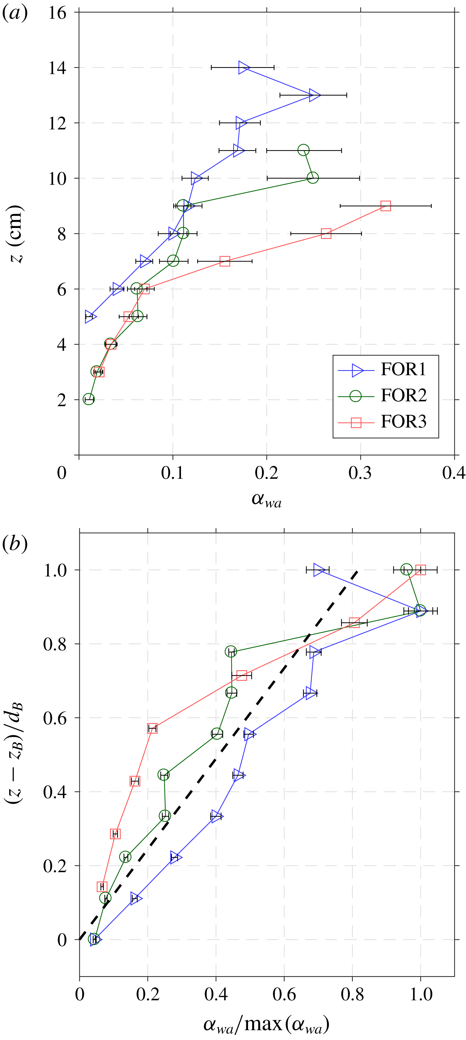
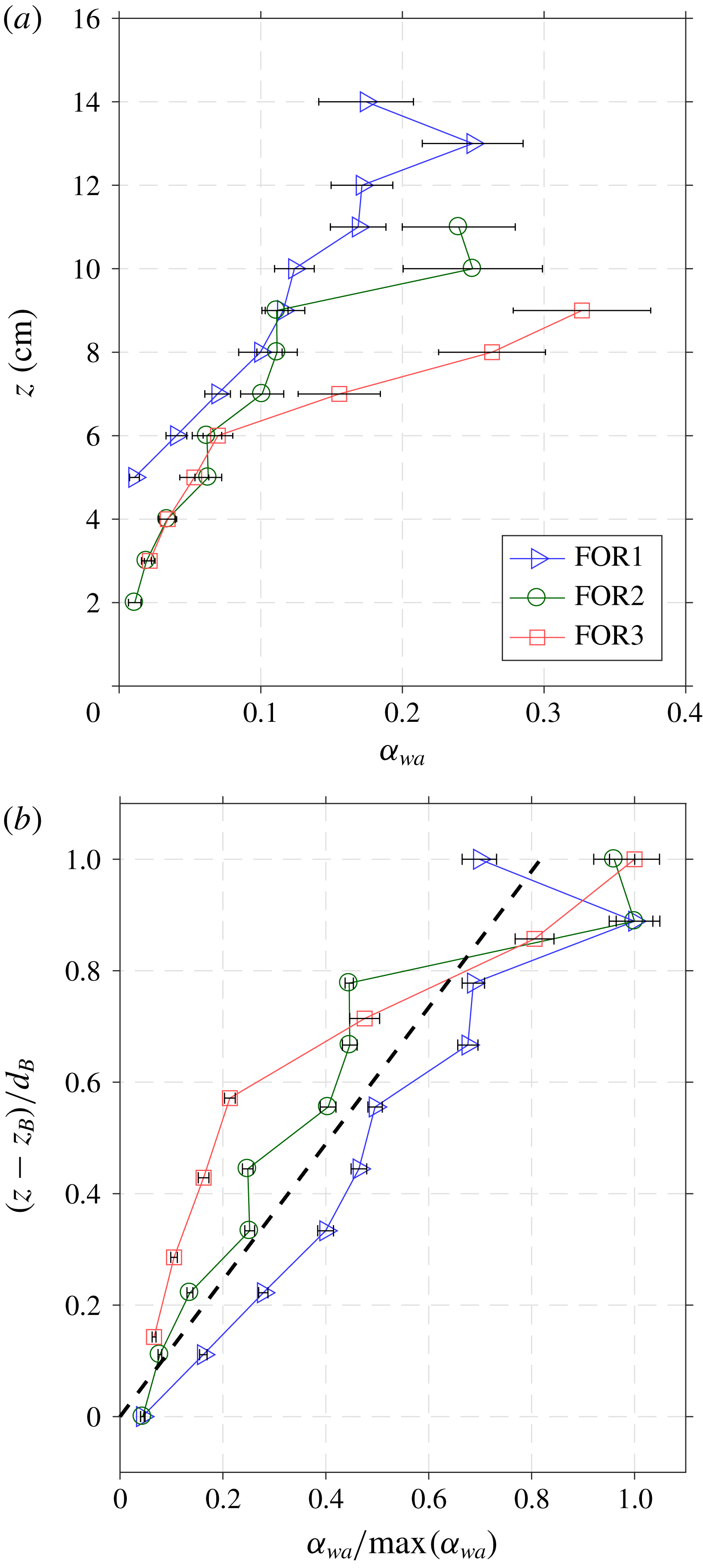
Vertical profiles of (a) wave-averaged void fraction (
 $\unicode[STIX]{x1D6FC}_{wa}$
) and (b) corresponding normalized wave-averaged void fraction. The void fraction is normalized by the maximum void fraction and the vertical axis is shifted with the penetration depth
 $(z_{B})$
and then normalized by the cloud thickness
 $(d_{B})$
at each FOR station. The thick dashed line in (b) is a linear least-squares fit over all the data points, expressed as
 $\unicode[STIX]{x1D6FC}_{wa}/\text{max}(\unicode[STIX]{x1D6FC}_{wa})=0.82(z-z_{B})/d_{B}$
. The error bars are standard deviations of the averaged quantities.
Temporal evolution of void fraction at (a) FOR station 1 (
 $x/L=0.50$
), (b) FOR station 2 (
 $x/L=1.00$
) and (c) FOR station 3 (
 $x/L=1.55$
). The dashed line is the contour boundary of
 $\langle \unicode[STIX]{x1D6FC}\rangle =0.2$
, and the solid line is the contour boundary of
 $\langle \unicode[STIX]{x1D6FC}\rangle =0.1$
. (d) Estimated bubble plume thickness at each FOR station.
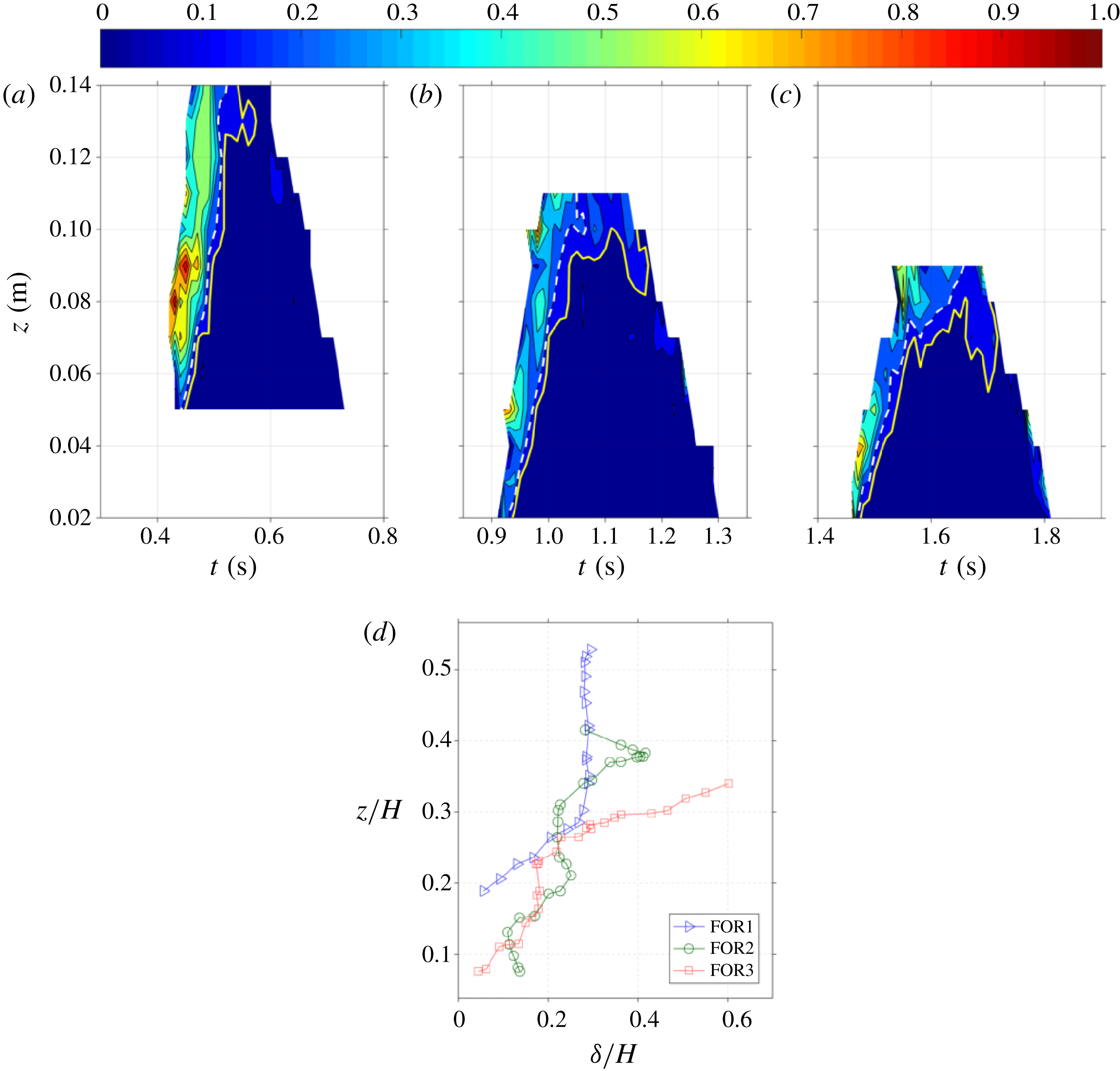
Figure 9(a) shows the vertical profiles of the wave-averaged void fraction measurements at FOR stations 1 (
 $x=0.5L$
), 2 (
 $x=L$
) and 3 (
 $x=1.55L$
); the corresponding maximum wave-averaged void fraction at each FOR station is 0.25, 0.25 and 0.33, respectively. In addition, the bubble cloud thicknesses (i.e. the vertical distance from the highest to the lowest edges of the cloud) are 7–9 cm. The cloud thickness was found to depend on the wind speed (the thickness increases with the increase of wind speed in general) and vary from 5 cm to 17 cm (Anguelova & Huq Reference Anguelova and Huq2012). These measured bubble cloud thicknesses also agree with those reported in Koga (Reference Koga1982), Thorpe (Reference Thorpe1982) and Kalvoda et al. (Reference Kalvoda, Xu and Wu2003). Rojas & Loewen (Reference Rojas and Loewen2010) measured the time-averaged void fractions of 0.17, 0.29, 0.20 and 0.26 at
 $x/L=0.31$
, 0.57, 0.83 and 1.08. In their study, instantaneous void fractions were averaged over the time interval only when the void fraction was less than 0.5 and, at each horizontal location, void fraction measurements were taken at only one vertical location, determined by the occurrence of the largest number of bubbles. The present study (
 $ka=0.45$
,
 $H=0.265~\text{m}$
) may be directly comparable to that of Rojas & Loewen (Reference Rojas and Loewen2010) because of the similar wave properties used
 $(ka=0.38,H=0.200~\text{m})$
in their study. The measured maximum void fraction of 0.25 in the present study is similar to that measured by Rojas & Loewen (Reference Rojas and Loewen2010) at
 $x/L=0.5$
and 1.0, but reaches 0.33 at
 $x/L=1.5$
in the present study (no data from Rojas & Loewen at this location). However, void fraction estimates by Leifer & de Leeuw (Reference Leifer and de Leeuw2006) under wind-generated spillers are lower than our values by one to two orders of magnitude, partly because their void fraction estimates are not time-averaged values. It is expected that less air entrainment occurs during breaking for less energetic spillers. The wavelength and the wave height of the wind-generated spillers in Leifer & de Leeuw (Reference Leifer and de Leeuw2006) are 1.3 m and 0.12 m, respectively; these are shorter than those in the present study. The discrepancy is supported by the void fraction comparison in Rojas & Loewen (Reference Rojas and Loewen2010) and Loewen, O’Dor & Skafel (Reference Loewen, O’Dor and Skafel1996). The latter under very gentle spillers has void fraction approximately two orders of magnitude lower than that of the former under similar spillers as in the present study.
Figure 9(b) shows the normalized vertical profiles of the wave-averaged void fraction at the three FOR stations. At each station, the void fraction was normalized by the corresponding maximum void fraction, and the vertical axis was shifted with the penetration depth
 $z_{B}$
and then normalized by the corresponding cloud thickness
 $d_{B}$
. Figure 9(b) suggests that the normalized void fractions are self-similar, even though they are one wavelength apart at
 $x=0.5L$
,
 $1.0L$
and
 $1.55L$
. The normalized void fraction can be formulated as
 $$\begin{eqnarray}\unicode[STIX]{x1D6FC}_{wa}/\text{max}(\unicode[STIX]{x1D6FC}_{wa})=0.82(z-z_{B})/d_{B}.\end{eqnarray}$$
The self-similar behaviour was also reported in the first, second and third splash-ups for plunging breaking waves in deep water by Lim et al. (Reference Lim, Chang, Huang and Na2015).
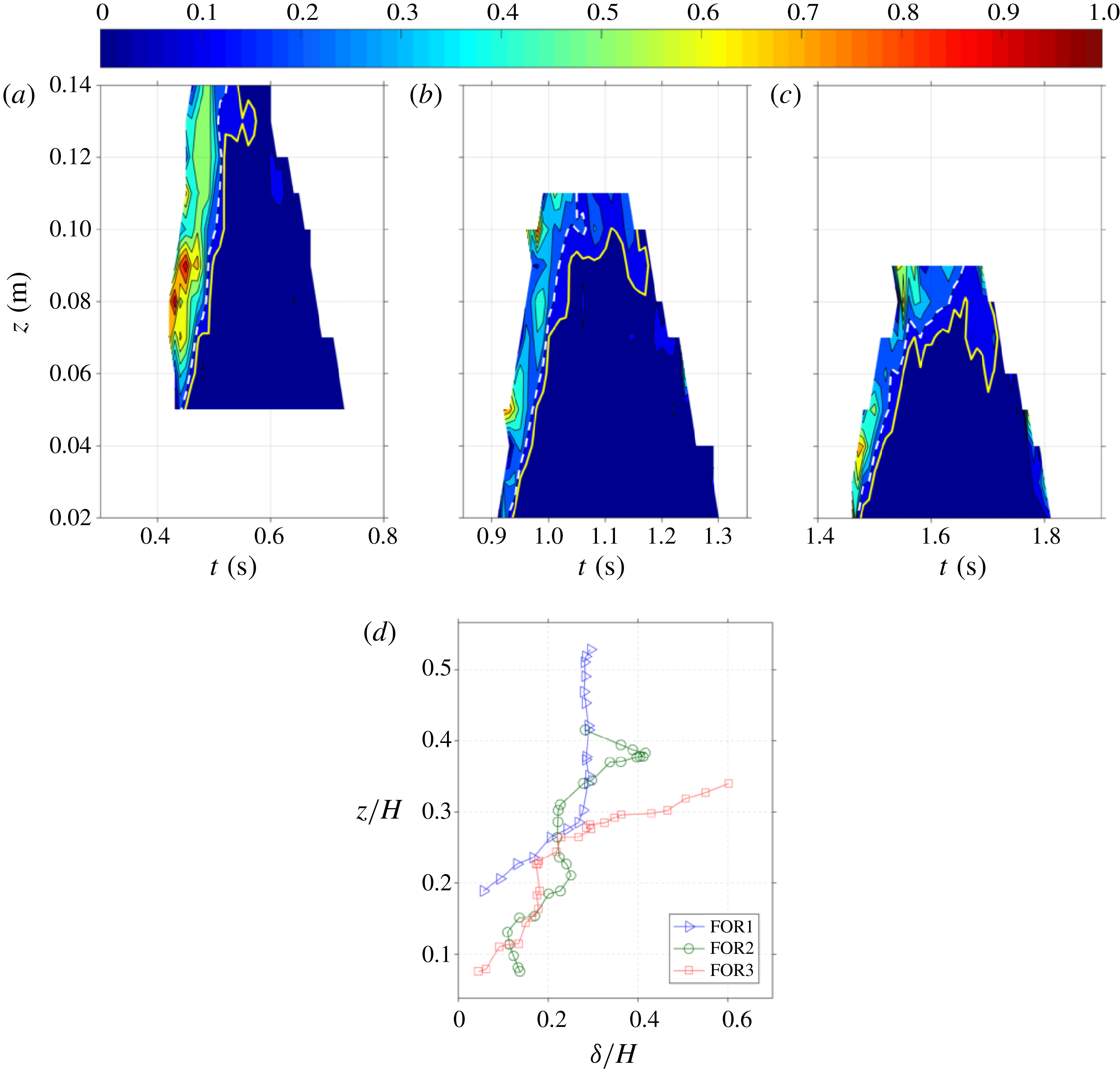
Figure 10 shows the temporal evolution of void fraction at each FOR station. The contours were obtained with a temporal resolution of 0.01 s and a spatial resolution of 10 mm. At FOR station 1
 $(x/L=0.5)$
, a void fraction higher than 0.6 is found in the lower half of the aerated region (at
 $t=0.43{-}0.47~\text{s}$
or
 $t/T=0.39{-}0.43$
in figure 10
a). In the upper half of the aerated region, the void fraction is relatively lower (around 0.4–0.5). Bubbles are concentrated near the shear zone and fragmented during this initial phase. Leifer & de Leeuw (Reference Leifer and de Leeuw2006) refer to this as the ‘injection phase’ when bubbles are advected downwards after the bubble plume is formed and before the bubbles rise. We believe that the high void fraction in the lower half of the plume is strongly related to the injection phase.
At FOR station 2
 $(x/L=1.0)$
, the contour in figure 10(b) shows that the discrepancy in void fraction between the upper half and the lower half of the aerated region is less distinguishable as moderately high void fraction appears sporadically within the region. At this stage, the bubble plume is likely to be in transition from the ‘rise phase’ (Leifer & de Leeuw Reference Leifer and de Leeuw2006) to the ‘senescence phase’, when the aerated region is mixed with dispersed larger bubbles that are rising due to buoyancy and smaller bubbles that are left at deeper locations. During the rise phase, the dominant advective process is buoyant rise for the larger bubbles in the plume; while during the senescence phase, turbulence and wave motion are important (Leifer & de Leeuw Reference Leifer and de Leeuw2006). During this transition phase, buoyancy, turbulence and wave motion are likely to affect the trajectories of the bubbles, resulting in the unorganized aeration levels within the region as shown in figure 10(b).
At FOR station 3
 $(x/L=1.55)$
, figure 10(c) may indicate that the majority of the larger bubbles have approached or risen and burst at the free surface, but the remaining smaller bubbles rise more slowly. The highly aerated layer (the warm colour region centred at around
 $z=0.08~\text{m}$
) at the left face of figure 10(a) initially stretched vertically with high void fraction, then gradually deformed into two separate patches – centred at around
 $z=0.05~\text{m}$
and
 $z=0.10~\text{m}$
in figure 10(b) and then around
 $z=0.04~\text{m}$
and
 $z=0.09~\text{m}$
in figure 10(c) – with moderate void fraction divided by a relatively lower aerated area in between the patches. This feature was not observed in the plunging breakers (Lim et al.
Reference Lim, Chang, Huang and Na2015; Na et al.
Reference Na, Chang, Huang and Lim2016). Leifer & de Leeuw (Reference Leifer and de Leeuw2006) referred this to the ‘senescence phase’. In the present spillers, once the larger bubbles rise to the surface, the remaining smaller bubbles rise at their relatively slow velocities and persist within the cloud. In contrast, in plungers, the plunging jets continuously introduce large bubbles from the splash-ups and breaking-up of entrapped air cavities. The large bubbles rise faster and scavenge the smaller, slowly rising bubbles, leaving a relatively lower number of smaller bubbles (Anguelova & Huq Reference Anguelova and Huq2018).
Blenkinsopp & Chaplin (Reference Blenkinsopp and Chaplin2007) used a threshold void fraction of 0.5 under plunging breaking waves to separate the highly aerated region (splash-up) above the free surface and moderately aerated region (impinging) below the free surface. As the void fraction level is lower in the present spilling breakers, we used a threshold of
 $\langle \unicode[STIX]{x1D6FC}\rangle =0.2$
in figure 10 (shown as a dashed line) to approximately mask the weakly aerated region. For each vertical measurement location, the time elapsed from detecting the arrival of the wave front to this dashed line is considered as the duration when the probe is in an ‘active bubble plume’. Lamarre & Melville (Reference Lamarre and Melville1992), Stansell & MacFarlane (Reference Stansell and MacFarlane2002) and Anguelova & Huq (Reference Anguelova and Huq2012) reported that the horizontal velocity of the bubble plume normalized by the phase speed of the wave is between 0.5 and 1. The mid-value of 0.75 was used to approximate the bubble plume horizontal thickness
 $\unicode[STIX]{x1D6FF}$
. The time interval in which we assumed that the plume is moving with a speed of
 $0.75C$
is essentially the coloured region in figure 10 from the front surface (the left surface) to the yellow solid line (with a mean void fraction = 0.1) in each panel. The mean time interval used is
 $0.07T$
,
 $0.11T$
and
 $0.10T$
at FOR station 1, 2 and 3, respectively. Figure 10(d) shows the bubble plume thickness at the three FOR stations. At FOR station 1, the vertical profile of the thickness is ‘curving upwards’ (shaped like the right half of
 $U$
) from the lower boundary to approximately
 $z/H=0.3$
, above which the bubble plume thickness is nearly constant. The plume thickness is in transition at FOR station 2, eventually transforming to ‘curving downwards’ (shaped like the left half of an upside-down U) at FOR station 3 after roughly one wavelength downstream from FOR station 1.
Rojas & Loewen (Reference Rojas and Loewen2010) reported that the minimum averaged void fraction ranges approximately from
 $\langle \unicode[STIX]{x1D6FC}\rangle =0.1$
to 0.2 at four measurement points under the spillers. We noticed that the contour lines of
 $\langle \unicode[STIX]{x1D6FC}\rangle =0.1$
and
 $\langle \unicode[STIX]{x1D6FC}\rangle =0.2$
show distinct evolution patterns, as shown specifically in figure 11(b,c) of Rojas & Loewen (Reference Rojas and Loewen2010). Accordingly, we used the lower bound of
 $\langle \unicode[STIX]{x1D6FC}\rangle =0.1$
(and below) as a criterion to define the weak bubble plume and the higher bound of
 $\langle \unicode[STIX]{x1D6FC}\rangle =0.2$
(and above) to define the active bubble plume. Thus, the volume of the active bubble plume was estimated by integrating the thickness over
 $z$
using the trapezoidal method based on the defined threshold of
 $\langle \unicode[STIX]{x1D6FC}\rangle =0.2$
. Similarly, the volume of the weak bubble plume was estimated using a threshold of
 $\langle \unicode[STIX]{x1D6FC}\rangle =0.1$
based on the same procedure as above. The estimated volumes of the active bubble plume per unit width are
 $0.0059~\text{m}^{2}$
,
 $0.0054~\text{m}^{2}$
and
 $0.0043~\text{m}^{2}$
at
 $x=0.5L$
,
 $x=L$
and
 $x=1.55L$
, respectively, while the estimated volumes of plume per unit width are
 $0.0078~\text{m}^{2}$
,
 $0.0078~\text{m}^{2}$
and
 $0.0062~\text{m}^{2}$
. Thus, the ratios of the weak bubble plume to the plume volume are 0.76, 0.69 and 0.69. The decreasing rate of these ratios is more significant at the earlier stage of breaking (
 $x/L=0.5$
–1.0), but insignificant at the later stage of breaking (
 $x/L=1.0$
–1.55). Lamarre & Melville (Reference Lamarre and Melville1992), Leifer & de Leeuw (Reference Leifer and de Leeuw2006) and Blenkinsopp & Chaplin (Reference Blenkinsopp and Chaplin2007) showed that the normalized volume of bubble plume follows an exponential decay. However, the number of measurement locations in the present study is too small to observe that.
Vertical profiles of time-averaged quantities: (a,d,g) void fraction; (b,e,h) turbulent intensity; and (c,f,i) swirling strength. (a–c) FOR station 1 (
 $x/L=0.50$
); (d–f) FOR station 2 (
 $x/L=1.00$
); and (g–i) FOR station 3 (
 $x/L=1.55$
). Horizontal lines indicate standard deviations. The horizontal error bars are standard deviations of the time-averaged quantities.
Based on the local velocity gradient tensors, the swirling strength
 $\unicode[STIX]{x1D713}$
, defined as the imaginary eigenvalue of the local deformation matrix
 $$\begin{eqnarray}DM=\left[\begin{array}{@{}cc@{}}\displaystyle \frac{\unicode[STIX]{x2202}u}{\unicode[STIX]{x2202}x} & \displaystyle \frac{\unicode[STIX]{x2202}u}{\unicode[STIX]{x2202}z}\\ \displaystyle \frac{\unicode[STIX]{x2202}w}{\unicode[STIX]{x2202}x} & \displaystyle \frac{\unicode[STIX]{x2202}w}{\unicode[STIX]{x2202}z}\end{array}\right]\end{eqnarray}$$
(Zhou et al.
Reference Zhou, Adrian, Balachandar and Kendall1999; Adrian, Christensen & Liu Reference Adrian, Christensen and Liu2000; Camussi Reference Camussi2002) can be computed. The swirling strength is proportional to the rotational speed of the vortical structures and has been proven useful in revealing the local vortical structures (Adrian et al.
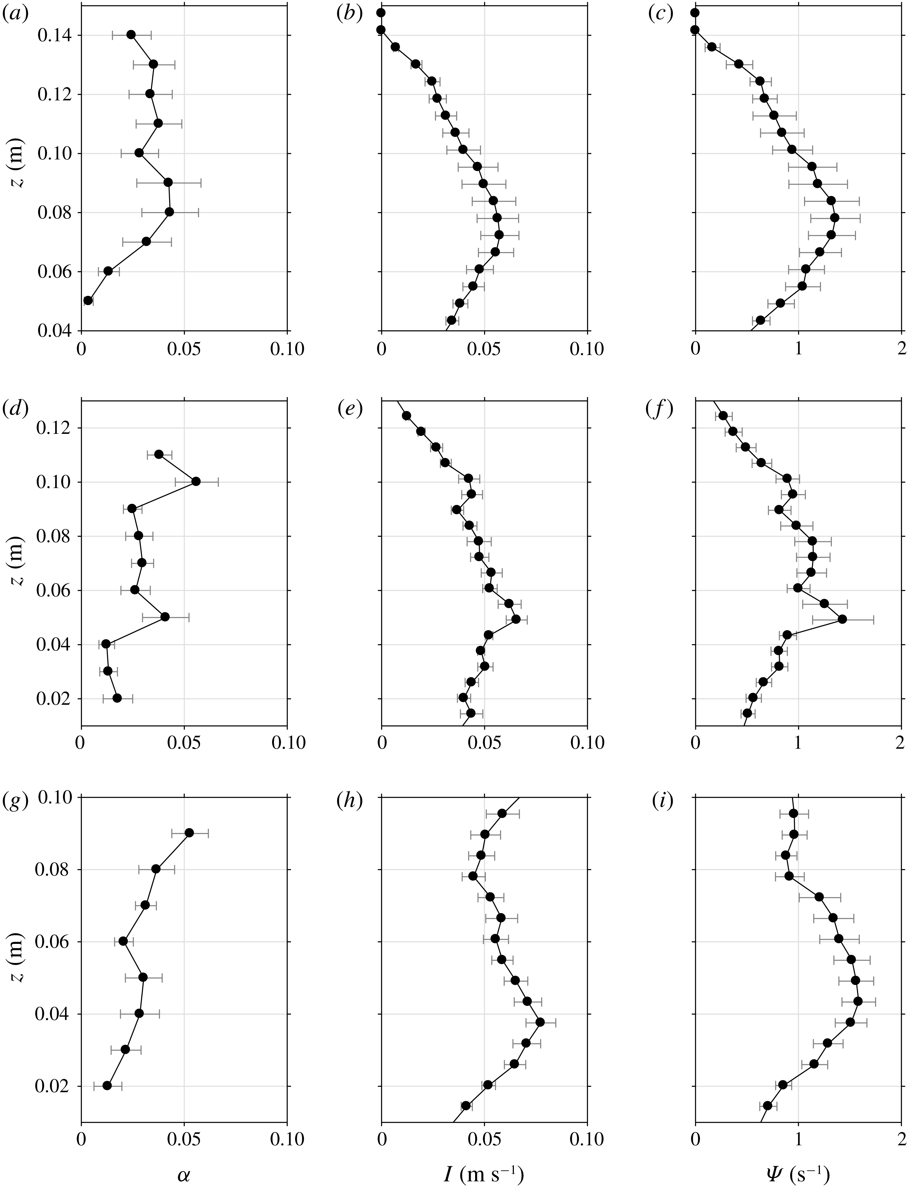
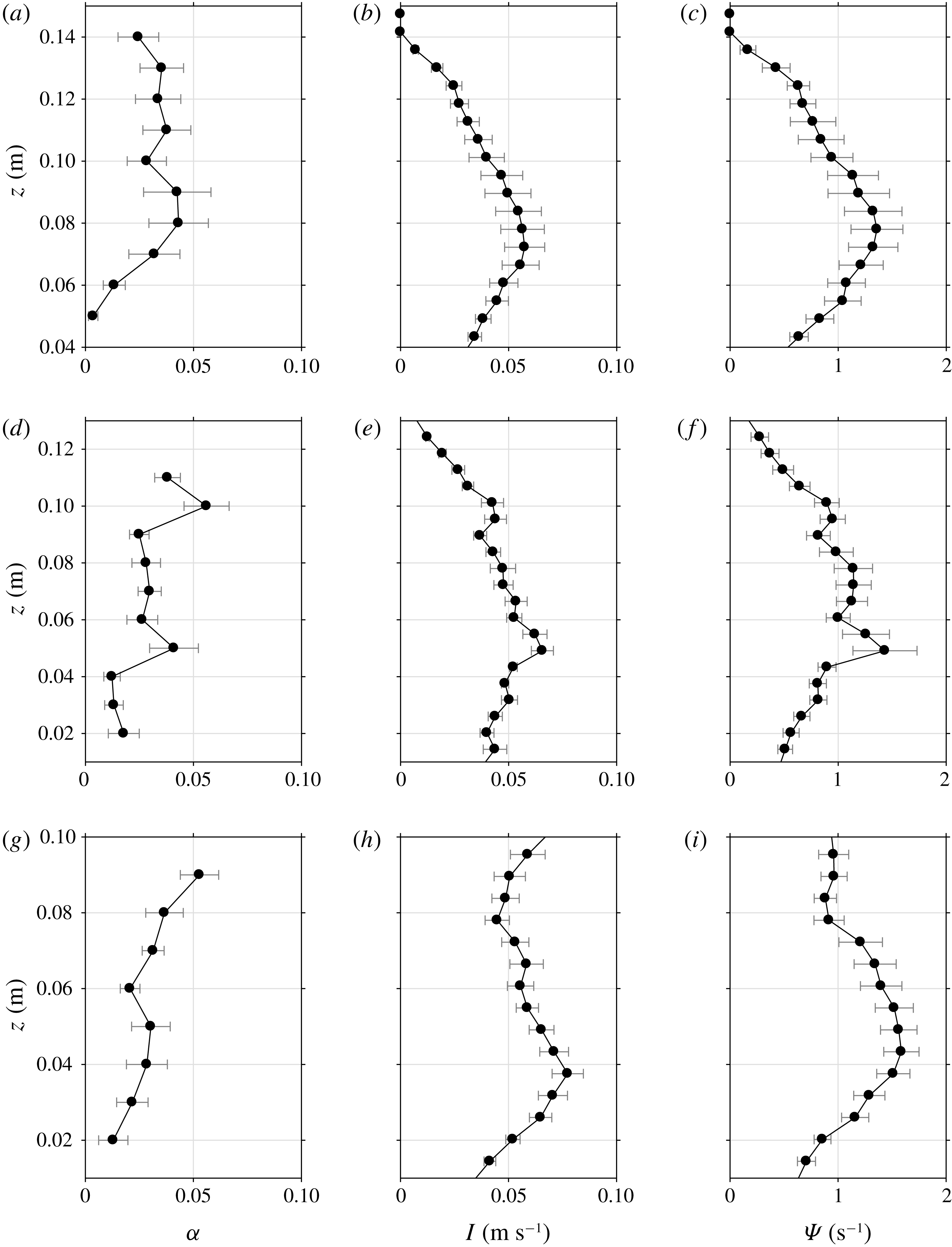
Reference Adrian, Christensen and Liu2000). Adrian et al. (Reference Adrian, Christensen and Liu2000) showed experimentally using PIV velocity maps that swirling strength is less noisy in identifying eddies and more effective in isolating eddies from local shear layers. On the contrary, vorticity identifies not only vortex cores but also any shearing motion present in the flow. Figure 11 shows the time-averaged quantities of void fraction, turbulent intensity and swirling strength in the active bubble plume region confined by the
 $\langle \unicode[STIX]{x1D6FC}\rangle =0.2$
threshold. A time-averaged quantity is defined as
 $$\begin{eqnarray}q_{ta}(x,z)=\frac{\displaystyle \int _{t_{tr}(x)}^{t_{tr}(x)+T}\unicode[STIX]{x1D709}(x,z,t)q(x,z,t)\,\text{d}t}{\displaystyle \int _{t_{tr}(x)}^{t_{tr}(x)+T}\unicode[STIX]{x1D709}(x,z,t)\,\text{d}t},\end{eqnarray}$$
where
 $q_{ta}$
is the time-averaged quantity (i.e. void fraction, turbulent intensity and swirling strength) and
 $\unicode[STIX]{x1D709}(x,z,t)=1$
when
 $\langle \unicode[STIX]{x1D6FC}\rangle \geqslant 0.2$
and
 $\unicode[STIX]{x1D709}(x,z,t)=0$
when
 $\langle \unicode[STIX]{x1D6FC}\rangle <0.2$
. As discussed in figure 11, the transition of the vertical profiles of void fraction from curving upwards to curving downwards can be seen in figure 11(a,d,g). The vertical profiles of void fraction, turbulent intensity and swirling strengths (especially the latter two) show depending trends and similar locations of the local peaks at all three FOR stations. In particular, the secondary local peaks located at
 $z=0.1~\text{m}$
at FOR station 2 are consistent among void fraction, turbulent intensity and swirling strengths in figure 11(d–f). These equivalent local peaks, caused by the weak jet impingement of the breaking waves, are barely visible at
 $z=0.13~\text{m}$
at FOR station 1. The apparent secondary local peak at FOR station 2 is probably caused by the mild overturning and subsequent jet impingement. Although this weak overturning was not evidently confirmed by the PIV and BIV images, it is supported by the local peak of
 $B$
near
 $t/T=0.9$
as shown in figure 3. At FOR station 3, the void fraction increases near the surface because of the risen bubbles due to buoyancy. This may in turn increase the magnitudes of turbulent intensity and swirling strength as shown in figure 11(g–i). The results imply that turbulent intensity is positively correlated with void fraction under spilling breaking waves. Lim et al. (Reference Lim, Chang, Huang and Na2015) also reported a strong correlation between turbulent intensity and void fraction in highly aerated plunging breaking waves. However, Deane & Stokes (Reference Deane and Stokes2002) argued that the coincidence of high void fraction with high turbulence in breaking waves may not be sufficient to conclude that the turbulent properties are strongly enhanced by void fraction. Note that the distribution of the swirling strength in figure 11 is very similar to that of the vorticity magnitude (not plotted in the figure).
Although the present study was performed in fresh water, its goal is to deepen our understanding of the wave breaking process and its induced air entrainment in open oceans. It is worth pointing out the potential effects of salinity on void fraction and bubble generation. Anguelova & Huq (Reference Anguelova and Huq2018) experimentally showed that salinity alters the bubble size and number by performing a single case of jet impingement to mimic a plunging breaker. The number of large bubbles and void fraction increase with salinity, reaching the maximum at salinity of
 $S=12{-}25~\text{g}~\text{kg}^{-1}$
. Both the number of large bubbles and void fraction decrease with further increase of salinity beyond
 $S=25$
. They referred this to a non-monotonic dependence of the number of bubbles and void fraction on salinity, which may explain the previously contradictory literature (Monahan & Zietlow Reference Monahan and Zietlow1969; Carey et al.
Reference Carey, Fitzgerald, Monahan and Wang1993; Monahan et al.
Reference Monahan, Wang, Wang and Wilson1994). Although Anguelova & Huq (Reference Anguelova and Huq2018) tested only one case, they further argued that the dependence of their results on various breaking strengths may not be significant based on Blenkinsopp & Chaplin’s (Reference Blenkinsopp and Chaplin2007, Reference Blenkinsopp and Chaplin2011) results.
4.2 Wave energy variation considering void fraction
Void fraction is essential for investigating the flow properties that involve fluid density variation, such as the mean kinetic energy, turbulent kinetic energy and potential energy in the present study. Lim et al. (Reference Lim, Chang, Huang and Na2015) showed that the discrepancy of estimated kinetic energy with and without considering void fraction reached 52 % under plunging breaking waves. They concluded that the mixture density of highly aerated flows such as breaking waves must be accounted for in estimating energy and dissipation. However, density variations have rarely been considered in experimental studies of wave breaking. This hurdle is probably caused by difficulties in measuring both velocities and void fraction (and hence the mixture density) simultaneously in experiments.
In the present study, the mean kinetic energy per unit water mass
 $(K)$
was obtained from the mean horizontal velocity
 $(U)$
and the mean vertical velocity
 $(W)$
with the assumption that the mean cross-tank velocity
 $(V)$
is zero, i.e.
 $$\begin{eqnarray}K={\textstyle \frac{1}{2}}(U^{2}+W^{2}).\end{eqnarray}$$
The corresponding turbulent kinetic energy
 $k$
was approximated as
 $$\begin{eqnarray}k=\frac{1.33}{2}(\langle u^{\prime \,2}\rangle +\langle w^{\prime \,2}\rangle )=\frac{1.33}{2}I_{2D}^{2},\end{eqnarray}$$
where the constant 1.33 accounts for the missing
 $y$
-direction velocity (e.g. Chang & Liu Reference Chang and Liu1999). Note that the factor of 1.33, suggested by Svendsen (Reference Svendsen1987) and used in many wave breaking studies, has been verified for surf-zone plunging breaking waves (Christensen Reference Christensen2006).
The period-averaged mean kinetic energy
 $(K_{pa})$
and turbulent kinetic energy
 $(k_{pa})$
considering void fraction are given as
 $$\begin{eqnarray}\left.\begin{array}{@{}c@{}}\displaystyle K_{pa}(x,z)=\frac{\displaystyle \int _{t_{tr}(x)}^{t_{tr}(x)+T}\unicode[STIX]{x1D6FF}(x,z,t)(1-\langle \unicode[STIX]{x1D6FC}\rangle )K(x,z,t)\,\text{d}t}{\displaystyle \int _{t_{tr}(x)}^{t_{tr}(x)+T}\,\text{d}t},\\ \displaystyle k_{pa}(x,z)=\frac{\displaystyle \int _{t_{tr}(x)}^{t_{tr}(x)+T}\unicode[STIX]{x1D6FF}(x,z,t)(1-\langle \unicode[STIX]{x1D6FC}\rangle )k(x,z,t)\,\text{d}t}{\displaystyle \int _{t_{tr}(x)}^{t_{tr}(x)+T}\,\text{d}t}.\end{array}\right\}\end{eqnarray}$$
Furthermore, the depth-integrated mean kinetic energy
 $(K_{di})$
and turbulent kinetic energy
 $(k_{di})$
were computed by integrating the corresponding period-averaged quantities from the bottom to the free water surface
 $(\unicode[STIX]{x1D702})$
as
 $$\begin{eqnarray}\left.\begin{array}{@{}c@{}}\displaystyle K_{di}(x)=\int _{-h}^{\unicode[STIX]{x1D702}(x)}K_{pa}(x,z)\,\text{d}z,\\ \displaystyle k_{di}(x)=\int _{-h}^{\unicode[STIX]{x1D702}(x)}k_{pa}(x,z)\,\text{d}z.\end{array}\right\}\end{eqnarray}$$
The total kinetic energy
 $(KE)$
can be obtained by summing the mean kinetic energy and turbulent kinetic energy, i.e.
 $KE=K_{di}+k_{di}$
. Note that in the present study the PIV measurement covered only from
 $z=-0.64h$
(equivalent to
 $0.28L$
) to the free surface. The missing values between
 $z=-0.64h$
and
 $z=-h$
can be interpolated in the integration but their contributions are insignificant and thus neglected.
In the present study, the potential energy
 $(PE)$
was determined using the free-surface elevation from the images with void fraction considered as follows:
 $$\begin{eqnarray}PE=\int _{-h}^{\unicode[STIX]{x1D702}}(1-\langle \unicode[STIX]{x1D6FC}\rangle )gz\,\text{d}z-\frac{1}{2}gh^{2}.\end{eqnarray}$$
Lim et al. (Reference Lim, Chang, Huang and Na2015) showed that the presence of aeration in plunging breakers led to an underestimated potential energy when using only the free-surface elevation measured by resistance wave gauges, whereas using only the free-surface elevation obtained from images led to an overestimated value.
Figure 12(a) compares the variation of period-averaged, depth-integrated mean kinetic energy (
 $K_{di}$
) and turbulent kinetic energy (
 $k_{di}$
) with and without considering void fraction. If void fraction is not considered, the mean kinetic energy would be overestimated by 23 %, 49 % and 43 % at the three FOR stations at
 $x=0.5L$
,
 $L$
and
 $1.55L$
, respectively. The corresponding ratios of
 $k_{di}/K_{di}$
are 3 %, 5 % and 7 % with void fraction considered. These ratios are significantly lower than the 25 % ratio at the first impingement in the plunging breaking waves reported by Lim et al. (Reference Lim, Chang, Huang and Na2015). Note that, without considering void fraction, the ratios of
 $k_{di}/K_{di}$
increase slightly to 4 %, 8 % and 10 % in the present study. In figure 12(a), if the mean kinetic energy at the pre-breaking region at
 $x/L=-0.14$
is used as a reference with void fraction considered, the mean kinetic energy decreases by 16 %, 45 % and 58 % at
 $x/L=0.5$
, 1.0 and 1.55, respectively.
(a) Comparison of depth-integrated mean kinetic energy (
 $K_{di}$
) and turbulent kinetic energy (
 $k_{di}$
) with and without considering void fraction. (b) Turbulent kinetic energy (
 $k_{di}$
) with and without considering void fraction.
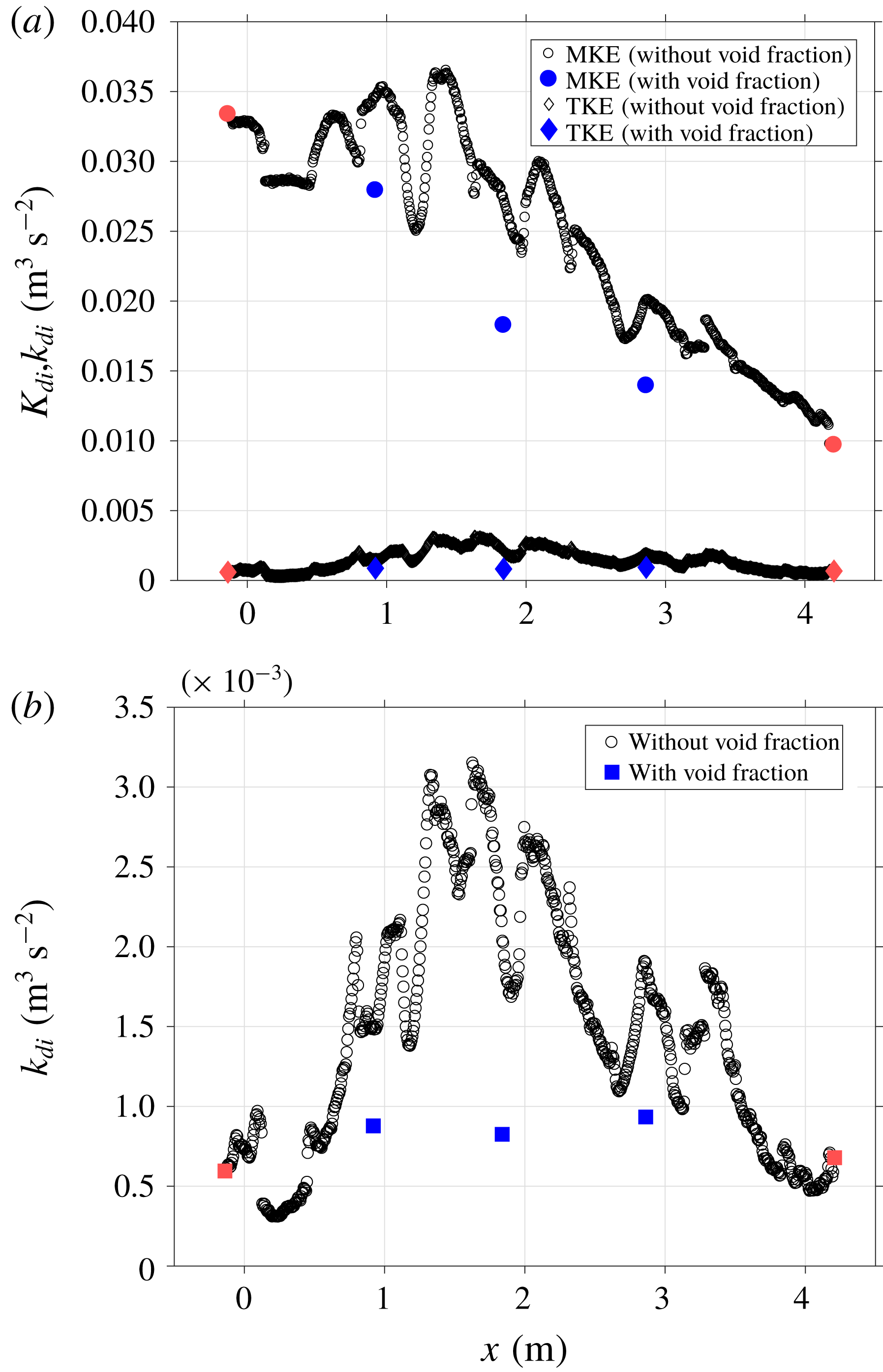
(a) Depth-integrated total kinetic energy (
 $KE=K_{di}+k_{di}$
) and (b) potential energy
 $(PE)$
with and without considering void fraction. (c) Total wave energy (
 $E_{\unicode[STIX]{x1D6FC}}=KE+PE$
) accounting for void fraction normalized by the corresponding pre-breaking wave energy (
 $E_{L}$
). The dashed line for
 $E_{\unicode[STIX]{x1D6FC}}/E_{L}$
is from the empirical formula
 $E_{\unicode[STIX]{x1D6FC}}/E_{L}=1.06\text{e}^{-0.55x/L}$
for
 $x/L>0.1$
and
 $E_{\unicode[STIX]{x1D6FC}}/E_{L}=1.0$
for
 $x/L\leqslant 0.1$
.
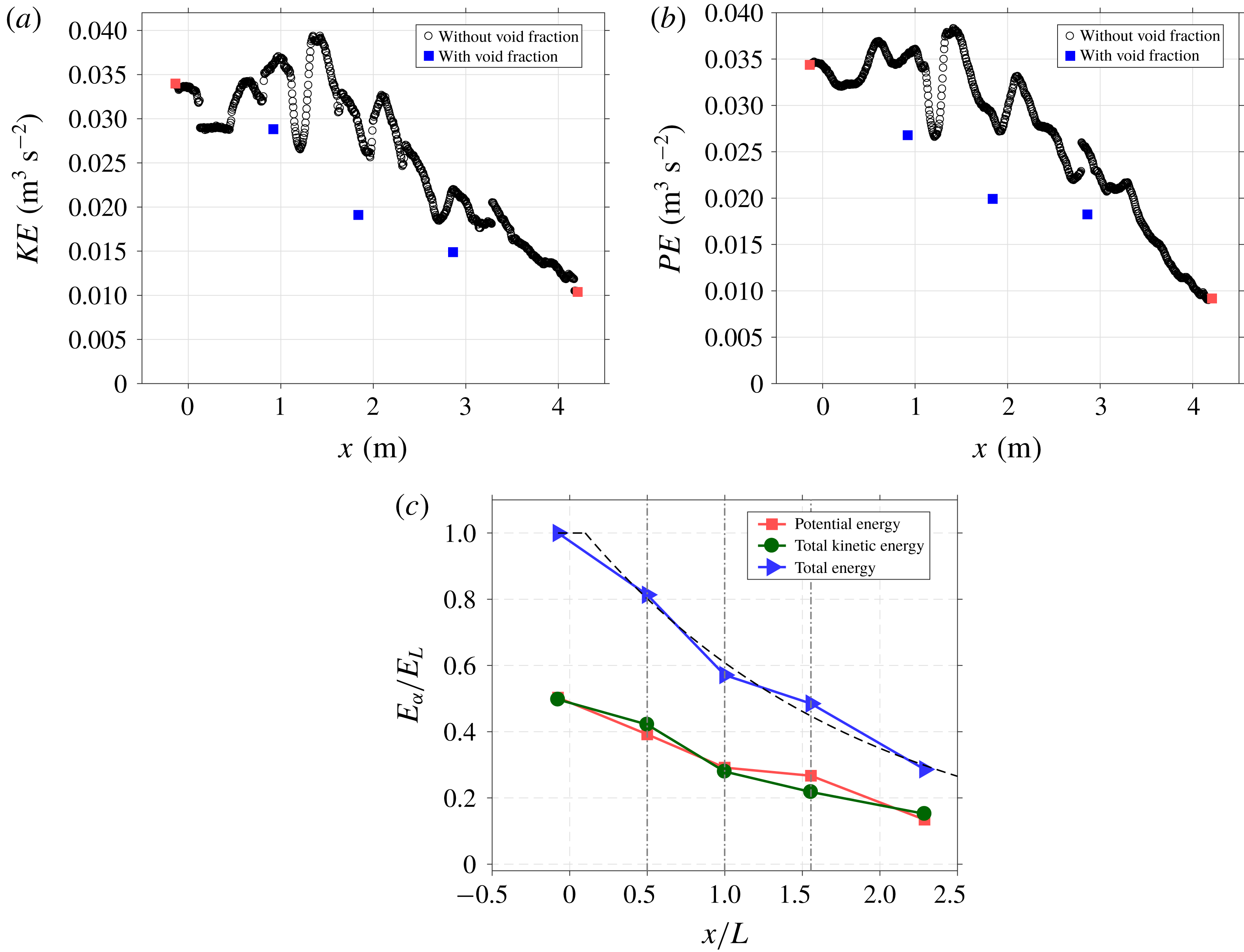
Figure 12(b) shows the variation of turbulent kinetic energy (
 $k_{di}$
) with and without considering void fraction. If void fraction is not considered, the turbulent kinetic energy would be overestimated by 69 %, 163 % and 104 % at the three FOR stations at
 $x=0.5L$
,
 $L$
and
 $1.55L$
, respectively, and probably more than 300 % at some other locations based on figure 12(b). Note that at the pre-breaking location of
 $x/L=-0.14$
the value of
 $k_{di}$
is not zero (also shown in figure 6). The value of
 $k_{di}$
then increases 47 %, 39 % and 57 % from the pre-breaking region, as shown in figure 12(b). The flow seems to maintain a somewhat even level of turbulent kinetic energy as the spilling wave propagates from
 $x=0.5L$
to
 $1.55L$
. This is consistent with the relatively even aeration levels measured at the three FOR stations shown in figure 9(a) and the implication between void fraction and turbulence intensity. Nevertheless, that trend is very different from the observation in plunging breaking waves, where the aeration level decreases significantly near
 $x=L$
(see figure 13a,b in Lim et al.
Reference Lim, Chang, Huang and Na2015).
Figure 13(a) shows the variation of depth-integrated total kinetic energy (
 $KE=K_{di}+k_{di}$
) with and without considering void fraction. If void fraction is not considered, the total kinetic energy would be overestimated by 25 %, 56 % and 47 % at
 $x/L=0.5$
, 1.0 and 1.55, respectively. With the density variation accounted for, the total kinetic energy drops 15 %, 44 % and 56 % at
 $x/L=0.5$
, 1.0 and 1.55, respectively, when compared to the total kinetic energy at the pre-breaking region at
 $x/L=-0.14$
. On the contrary, in plunging breaking waves the total kinetic energy increases by 18 % at
 $x/L=0.4$
because of the significant increase in the turbulent kinetic energy during the first impingement and splash-up processes (Lim et al.
Reference Lim, Chang, Huang and Na2015). This comparison shows that the production of the turbulent kinetic energy in the spilling breakers is not as significant as that in the plunging breakers.
Figure 13(b) compares the spatial variation of potential energy
 $(PE)$
with and without considering void fraction. If void fraction is not considered, the potential energy, based on video images, would be overestimated by 32 %, 47 % and 39 % at
 $x/L=0.5$
, 1.0 and 1.55, respectively. With the density variation accounted for, the potential energy drops 22 %, 42 % and 47 % at
 $x/L=0.5$
, 1.0 and 1.55, respectively, when compared to the pre-breaking potential energy at
 $x/L=-0.14$
. Interestingly, the potential energy has a significant decrease between
 $x/L=0$
and
 $x/L=1.0$
but only a slight decrease between
 $x/L=1.0$
and
 $x/L=1.55$
. Similarly, in plunging breaking waves, the potential energy has a significant decrease of approximately 32 % between
 $x/L=0.4$
and
 $x/L=0.8$
and a slight decrease of 2 % between
 $x/L=0.8$
and
 $x/L=1.1$
(Lim et al.
Reference Lim, Chang, Huang and Na2015).
Figure 13(c) shows the spatial variation of potential energy, total kinetic energy and total energy
 $(KE+PE)$
accounting for the mixture density. The total energy decreases relatively quickly before
 $x/L=1$
and then more slowly beyond that point. In particular, the total energy drops 19 %, 43 % and 52 % at
 $x/L=0.5$
, 1.0 and 1.55 when compared to the total energy at the pre-breaking region at
 $x/L=-0.14$
. The total energy is dissipated following an exponential decay similar to that under plunging breaking waves in Lim et al. (Reference Lim, Chang, Huang and Na2015). The wave energy variation considering void fraction under spilling breakers may be formulated as
 $$\begin{eqnarray}E_{\unicode[STIX]{x1D6FC}}/E_{L}=1.06\text{e}^{-0.55x/L}\quad \text{for }x/L>0.1,\end{eqnarray}$$
where
 $E_{\unicode[STIX]{x1D6FC}}$
is the breaking wave energy with void fraction considered and
 $E_{L}$
is the pre-breaking wave energy. For
 $x/L\leqslant 0.1$
,
 $E_{\unicode[STIX]{x1D6FC}}/E_{L}=1.0$
is assumed, based on the curve fitting. Note that this exponential decay rate of
 $-0.55$
in the equation is approximately one-half of the rate of
 $-1.17$
in the plunging breaking waves in Lim et al. (Reference Lim, Chang, Huang and Na2015).
The spatial variations of total kinetic energy and potential energy in figure 13(c) exhibit similarities which suggest that the equipartition assumption may be valid not only outside of the actively breaking zone, but also inside the active aerated region under the spilling breakers. In contrast, Lim et al. (Reference Lim, Chang, Huang and Na2015) showed that the equipartition assumption is not applicable during the highly aerated phase and is valid only beyond
 $x/L=2$
with a relatively low aeration level under the plunging breaking waves. Based on figure 13(c), approximately 65 % and 71 % of the total energy is dissipated at
 $x/L=2.0$
and 2.3, respectively.
Based on figure 13(c), the rate of loss of total energy (i.e. the non-dimensional slope
 $\text{d}(E_{\unicode[STIX]{x1D6FC}}/E_{L})/\text{d}(x/L)$
) for the spiller is milder near the breaking point at
 $x=0.5L$
when compared to that for the plunger in Lim et al. (Reference Lim, Chang, Huang and Na2015). The difference in the slope between the spiller and the plunger becomes less prominent near
 $x=1.5L$
. Of particular interest is that the magnitude of the slope showed an increase during the active breaking stage around
 $0.5L$
, followed by a decrease around
 $1.0L$
in both the spiller and the plunger. The measured data confirm the simulated results in Derakhti & Kirby (Reference Derakhti and Kirby2014) in which the dissipation rate increased during active breaking and decreased at the end of active breaking.
The ratio of potential energy to total energy has been known to depend on the breaking strength. Derakhti & Kirby (Reference Derakhti and Kirby2016) found that the ratio of potential energy density to total energy density,
 $PE/E$
, varied from approximately 0.6 in the pre-breaking stage to approximately 0.5 near the breaking onset with presence of breaking-induced bubbles. Derakhti & Kirby (Reference Derakhti and Kirby2016) suggested that
 $PE/E$
varies but is centred around 0.6 in the spiller. However, figure 13(c) in the present study shows that this ratio stays close to 0.5 (i.e. following equipartition) throughout the breaking process in the spiller. In the plunger, Lim et al. (Reference Lim, Chang, Huang and Na2015) reported that
 $PE/E$
decreases from 0.5 in the pre-breaking stage to around 0.4 near the onset. These are inconsistent with the reported values in Derakhti & Kirby (Reference Derakhti and Kirby2016). Additionally, a steep increase of
 $PE/E$
near
 $t/T=1$
was not observed in the present study.
5 Conclusions
In the current study, flow kinematics, turbulence, void fraction and the effects of void fraction were investigated based on laboratory measurements of spilling breaking waves. The spilling breakers were generated using a wave focusing technique; each wave train in a test run only generates one breaking event. Velocity fields were measured using a modified PIV technique while free-surface elevations were measured using both images and wave gauges. Void fraction profiles were measured using the FOR technique at three locations relative to the wavelength. Ensemble averaging was performed to obtain the mean and turbulence properties. Through combined velocity and void fraction measurements, the data uniquely highlight kinematic and dynamic properties of the multiphase flow, as well as characteristics of the flow structure in the highly aerated region under spilling breaking waves, where gravity is the predominant restoring force. The findings are mostly consistent with existing experimental studies and aligned with recent numerical simulations. The main findings are summarized and grouped into the following categories.
(1) Breaking onset. The normalized local wave period, defined as the time interval between two troughs – the front trough and the rear trough of the progressing breaker – linearly decreases in space. The phase speed based on the local position of maximum surface elevation is increased by 6 %. In addition, our results have confirmed the 0.85 threshold ratio reported in Barthelemy et al. (Reference Barthelemy, Banner, Peirson, Fedele, Allis and Dias2018) for the normalized energy flux at the wave crest for the wave to proceed irreversibly to break. We also measured the relationship between the breaking strength parameter and the non-dimensional rate of change of normalized energy flux at the crest at the breaking onset threshold. We found that it is consistent with the result based on numerical simulations presented in Derakhti et al. (Reference Derakhti, Banner and Kirby2018). Indeed, multiple increases of local energy exceeding the threshold were observed in the present spilling breakers after wave breaking. Through video images, the occurrences of very weak impingements of the overturning jets were coincident with those exceedances.
(2) Kinematics and turbulence. Near the breaking point where the wave front becomes vertical, the maximum horizontal velocity reaches
 $1.1C$
, agreeing with the findings of Duncan (Reference Duncan2001) under weak spilling breaking waves. The maximum magnitude of the horizontal velocity during the entire breaking process is
 $1.5C$
at
 $t/T=0.35$
. Close to the onset of breaking, a thin layer of turbulence is initiated at the crest. It later becomes thicker with increased turbulence intensity as the wave progresses. The measured vorticity fields show that a vortical region, located mainly below the toe immediately after breaking, stretches and extends to the crest above the toe as the breaking progresses. The wavelet-educed turbulent length scale inside the aerated region was found as
 $H/LS=5{-}12$
(i.e.
 $LS=2{-}5~\text{cm}$
in the present study). The length scale estimates are in agreement with the values reported in Longo (Reference Longo2009) and Huang et al. (Reference Huang, Hwung and Chang2010) in the surf-zone spillers with different wave parameters. The comparisons suggest that there may not be significant scale effects in the spilling breakers. The measured turbulence length scale under the current spilling breakers is also favourably comparable to the values under plunging breakers of similar physical dimensions in Na et al. (Reference Na, Chang, Huang and Lim2016).
(3) Void fraction and flow structures. The penetration depth of the aerated bubble cloud detected by FOR reaches 5, 2 and 2 cm at
 $x=0.5L$
,
 $L$
and
 $1.55L$
. The bubble cloud remains above the still-water level during the entire breaking process. It was found that the normalized void fraction is self-similar, even though the measurement locations are one wavelength apart at
 $x=0.5L$
,
 $L$
and
 $1.55L$
. The measured maximum wave-averaged void fraction levels are 0.25, 0.25 and 0.33 at these three locations. The temporal evolution of void fraction is compared to the four stages of bubble plume evolution proposed by Leifer & de Leeuw (Reference Leifer and de Leeuw2006). The void fraction profiles under the spilling breaking waves exhibit the characteristics of the ‘injection’, ‘rise’ and ‘senescence’ phases (Leifer & de Leeuw Reference Leifer and de Leeuw2006) under the spilling breakers. The measured data showed that the highly aerated layer shortly after breaking initially stretched vertically with high void fraction, then gradually deformed into two separate patches with moderate void fraction divided by a relatively lower aerated area in between the patches. This implies that, once the larger bubbles rise to the surface, the remaining smaller bubbles rise at their relatively slow velocities and persist within the cloud. In addition, the vertical profiles among void fraction, turbulent intensity and swirling strengths show dependent trends with the coincident local peaks, despite minor variations.
(4) Wave energy considering void fraction. The spatial variations of mean kinetic energy, turbulent kinetic energy and potential energy are compared with and without considering void fraction. These quantities are considerably overestimated if void fraction is not accounted for. The total kinetic energy is overestimated by approximately 60 % and the potential energy is overestimated by approximately 40 % at
 $x=L$
. When void fraction is considered, the kinetic energy shows a decreasing trend under the current spilling breaking waves. In contrast, in plunging breaking waves the kinetic energy increases by approximately 18 % at
 $x/L=0.4$
, in comparison to a 15 % decrease at
 $x/L=0.5$
in the present spilling breakers. The discrepancy is caused by the significant increase of the turbulent kinetic energy during the first impingement and splash-up processes in plunging breakers (Lim et al.
Reference Lim, Chang, Huang and Na2015). In the spilling breaker, the spatial distribution of total wave energy was observed to follow an exponential decay
 $E_{\unicode[STIX]{x1D6FC}}/E_{L}=1.06\text{e}^{-0.55x/L}$
for
 $x/L>0.1$
. It showed that the rate of total energy dissipation with respect to its horizontal propagation distance is enhanced at
 $0.5L$
and decreased at
 $1.0L$
. In comparison to plunging breaking waves, the total energy is dissipated following a similar exponential decay rate, except that the rate is approximately 50 % slower. The equipartition assumption remains applicable before and during the entire breaking process in the present spilling breakers, whereas the assumption becomes invalid shortly after wave breaking occurs in the plunging breakers (Lim et al.
Reference Lim, Chang, Huang and Na2015). The ratio of potential energy to the total energy,
 $PE/E$
, remained close to 0.5 in the spiller from pre-breaking
 $(x/L<0)$
to the measurement domain of
 $x/L=2.2$
.
Acknowledgements
The authors wish to express thanks for the partial financial support provided by the Offshore Technology Research Center (OTRC) through its Industry Consortium under the project entitled ‘Implementation of Bubble Image Velocimetry in OTRC Wave Basin’. The data used in generating the results in this study will be available upon request by contacting the corresponding author (K.A.C.) at kchang@tamu.edu.