1 Introduction
Lagrangian stochastic models are widely used to describe complex turbulent flows (Pope Reference Pope2000; Fox Reference Fox2003; Chibbaro & Minier Reference Chibbaro and Minier2014), and are of particular relevance for turbulent dispersion (Wilson & Sawford Reference Wilson and Sawford1996), reactive flows (Pope Reference Pope1985; Fox Reference Fox2003) and inertial particles (Minier & Peirano Reference Minier and Peirano2001; Peirano et al. Reference Peirano, Chibbaro, Pozorski and Minier2006; Minier Reference Minier2016). They are also appealing when Lagrangian properties are under investigation (Yeung & Pope Reference Yeung and Pope1989; Mordant et al. Reference Mordant, Delour, Léveque, Arnéodo and Pinton2002; Meneveau Reference Meneveau2011; Watteaux et al. Reference Watteaux, Sardina, Brandt and Iudicone2019).
Lagrangian stochastic models produce collections of synthetic trajectories that reproduce the statistical and, in some less accurate weak sense (i.e. the convergence is assured only in distribution), the dynamical properties of particles advected by the flow (Pope Reference Pope1985; Kloeden & Platen Reference Kloeden and Platen1992). In this framework, stochastic models focus generally on the dynamics of the one-point and one-time probability density function (PDF) of the state vector of the system (Pope Reference Pope2000).
The choice of the relevant variables for the model (i.e. the appropriate state vector) is key to an accurate description of a given turbulent flow. In particular, it is essential to retain enough variables to have a state vector that can be described as Markovian (Onsager & Machlup Reference Onsager and Machlup1953; Gardiner Reference Gardiner1990; Marconi et al. Reference Marconi, Puglisi, Rondoni and Vulpiani2008). Since these models are mainly conceived to tackle general non-homogeneous flows relevant for applications, the state vector is usually limited to the position and velocity of the fluid particles  $(\boldsymbol{x},\boldsymbol{U})$. These observables are modelled as a diffusion process, which is justified in relation to Kolmogorov theory (Pope Reference Pope1994a). A variety of models have been proposed for such a process (Lundgren Reference Lundgren1969; Pope Reference Pope1981), but one of the more widely accepted is the so-called generalised Langevin model, which reads as
 $$\begin{eqnarray}\displaystyle \left.\begin{array}{@{}l@{}}\text{d}x_{i}=U_{i}\,\text{d}t,\\[3.0pt] \text{d}U_{i}=-{\displaystyle \frac{1}{\unicode[STIX]{x1D70C}}}{\displaystyle \frac{\unicode[STIX]{x2202}\langle P\rangle }{\unicode[STIX]{x2202}x_{i}}}\,\text{d}t+\unicode[STIX]{x1D60E}_{ij}(U_{j}-\langle U_{j}\rangle )\,\text{d}t+\sqrt{C_{0}\langle \unicode[STIX]{x1D716}\rangle }\,\text{d}W_{i},\end{array}\right\} & & \displaystyle\end{eqnarray}$$
where  $\boldsymbol{W}$ is an isotropic Wiener process (Gardiner Reference Gardiner1990) and
 $$\begin{eqnarray}\unicode[STIX]{x1D60E}_{ij}=-\frac{1}{T_{L}}\unicode[STIX]{x1D6FF}_{ij}+\unicode[STIX]{x1D60E}_{ij}^{a}\quad \text{and}\quad T_{L}=\left(\frac{1}{2}+\frac{3}{4}C_{0}\right)^{-1}\frac{k}{\langle \unicode[STIX]{x1D716}\rangle },\end{eqnarray}$$
where  $\unicode[STIX]{x1D60E}_{ij}^{a}$ is a traceless matrix with the dimension of the inverse of time,
 $k(\boldsymbol{x})$ is the turbulent kinetic energy,
 $\langle \unicode[STIX]{x1D716}\rangle (\boldsymbol{x})=\unicode[STIX]{x1D708}\langle |\unicode[STIX]{x1D735}\boldsymbol{u}|^{2}\rangle$ is the average dissipation rate and
 $C_{0}$ is a dimensionless constant of the model. The specification of
 $C_{0}$ and
 $\unicode[STIX]{x1D60E}_{ij}$ define the particular model.
These models have some limitations, and their validity may become questionable in some circumstances. In particular, in stationary isotropic turbulence the autocorrelation of the velocity for such models is given by (Pope Reference Pope2000)
 $$\begin{eqnarray}\unicode[STIX]{x1D70C}(s)=\frac{\langle U(t)U(t+\unicode[STIX]{x1D70F})\rangle }{\langle U^{2}\rangle }=\exp \left(\frac{-|s|}{T_{L}}\right).\end{eqnarray}$$
This formula shows that the autocorrelation is non-differentiable at the origin, reflecting the fact that the velocity process is not differentiable. Only one time scale, namely  $T_{L}$ that is related to large energy-containing scales, is included in the model, and there is no Reynolds-number effect. Indeed, the separation of time scales
 $\unicode[STIX]{x1D70F}_{\unicode[STIX]{x1D702}}\ll T_{L}$, where
 $\unicode[STIX]{x1D70F}_{\unicode[STIX]{x1D702}}$ is the Kolmogorov time scale
 $\unicode[STIX]{x1D70F}_{\unicode[STIX]{x1D702}}\equiv (\unicode[STIX]{x1D708}/\langle \unicode[STIX]{x1D716}\rangle )^{1/2}$, allows these models to neglect high time–frequency behaviour, and limit the state vector to fluid particle position and velocity. This criterion is no longer met at low Reynolds numbers, with the Reynolds number defined as
 $Re=UL/\unicode[STIX]{x1D708}$, where
 $U$ and
 $L$ are typical velocity and length of large scales and
 $\unicode[STIX]{x1D708}$ is the kinematic viscosity. This assumption is not valid everywhere in a turbulent boundary layer, where the characteristic time scale of the flow in the near-wall region is of the order of the Kolmogorov scale. In this case, there is not a separation of scales sufficient to justify the Markovian description of the process
 $(\boldsymbol{x},\boldsymbol{U})$.
Some proposals have been made to address these issues in isotropic turbulence (Krasnoff & Peskin Reference Krasnoff and Peskin1971; Sawford Reference Sawford1991) by introducing a second time scale, which consequently introduces Reynolds-number dependence. Furthermore, experimental measurements of Lagrangian fluid acceleration in isotropic flows (Voth, Satyanarayan & Bodenschatz Reference Voth, Satyanarayan and Bodenschatz1998; Voth et al. Reference Voth, La Porta, Crawford, Alexander and Bodenschatz2002; Mordant, Lévêque & Pinton Reference Mordant, Lévêque and Pinton2004b) have motivated several models with the purpose of fitting the experimental data, but without a sound link to turbulence theory (Gotoh & Kraichnan Reference Gotoh and Kraichnan2004), with the notable exception of Lamorgese et al. (Reference Lamorgese, Pope, Yeung and Sawford2007). An important step forward has been taken by Pope (Reference Pope2002), who has proposed the use of a general diffusion stochastic model for fluid particle velocity and acceleration, and has considered in detail the case of homogeneous anisotropic turbulence. The goal of that work was not to propose a specific model, but rather to show that a diffusion process may reproduce quite well the direct numerical simulation (DNS) data if coefficients are correctly prescribed. However, no attempt has been made to develop a consistent model for general non-homogeneous flows, although this is the more realistic and relevant situation for applications.
The aim of the work reported here is to propose a first model that includes the acceleration of fluid particles for the general case of statistical inhomogeneous turbulence, and it follows recent experimental and DNS measurements of the acceleration of tracer particles in a turbulent channel flow at high Reynolds number (Stelzenmuller et al. Reference Stelzenmuller, Polanco, Vignal, Vinkovic and Mordant2017). The model is developed in the general framework of a diffusion process for the fluid particle velocity and acceleration (Pope Reference Pope2002), and can be applied also to statistical unsteady flows, even though the present work is focused on a statistical stationary channel flow. The coefficients of the model are not constrained by measurements, but rather on the basis of Kolmogorov theory and by the general analysis of the behaviour of the statistical moments, notably the Reynolds stresses, which can be extracted from the model. In the simplest case of isotropic flows, the model reverts to one that has been previously proposed (Krasnoff & Peskin Reference Krasnoff and Peskin1971; Sawford Reference Sawford1991). In non-homogeneous flows, when the acceleration can be considered as a fast process, i.e. when the observation scale is much larger than the characteristic acceleration scale, the model is consistent instead with the standard Langevin models for the fluid velocity given by (1.1). The resulting model therefore fulfils the criteria set down to characterise an acceptable model for general applications (Pope Reference Pope2000; Minier, Chibbaro & Pope Reference Minier, Chibbaro and Pope2014), and thus it could be applied to realistic flows of practical interest. Still, limitations inherent to the present approach are expected to require some improvements, at least in specific cases and for particular questions. Some possible ameliorations are discussed in the conclusions.
As well as being interesting in its own right, we also regard the present model as an intermediate step in the development of an improved Lagrangian stochastic model for inertial particles. In particular, the possible Reynolds number dependency has not yet been considered for such phenomena.
The paper is organised as follows. In § 2, we propose the new theoretical model and how to specify the coefficients of the governing equations. The different limit cases are also discussed. In § 3, the numerical approach is analysed, and we describe the numerical scheme developed to deal with the set of stochastic equations, which is stiff. In § 4, the results are reported: mean, variance and PDF of the acceleration components are compared against DNS and experimental data. A discussion and conclusions are given in § 5.
2 Theoretical model
In this work, we develop a Lagrangian stochastic model that consists of an ordinary differential equation for  $\boldsymbol{U}$, which models the exact fluid particle velocity
 $\boldsymbol{U}^{+}$, and a stochastic differential equation (SDE) for an acceleration variable
 $\boldsymbol{A}$, which models the exact acceleration:
 $$\begin{eqnarray}\boldsymbol{A}^{+}=\frac{\text{d}\boldsymbol{U}^{+}}{\text{d}t}=\boldsymbol{A}[\boldsymbol{X}^{+}(t),t],\end{eqnarray}$$
where  $\boldsymbol{X}^{+}(t)$ is the position of the fluid particle. The acceleration can be decomposed into its mean and fluctuating parts, based on the mean (
 $\langle P\rangle ,\langle \boldsymbol{U}\rangle$) and fluctuating (
 $p^{\prime },\boldsymbol{u}$) components of the pressure and velocity:
 $$\begin{eqnarray}A_{i}=-\frac{1}{\unicode[STIX]{x1D70C}}\frac{\unicode[STIX]{x2202}\langle P\rangle }{\unicode[STIX]{x2202}x_{i}}-\frac{1}{\unicode[STIX]{x1D70C}}\frac{\unicode[STIX]{x2202}p^{\prime }}{\unicode[STIX]{x2202}x_{i}}+\unicode[STIX]{x1D708}\frac{\unicode[STIX]{x2202}^{2}\langle U_{i}\rangle }{\unicode[STIX]{x2202}x_{k}\unicode[STIX]{x2202}x_{k}}+\unicode[STIX]{x1D708}\frac{\unicode[STIX]{x2202}^{2}u_{i}}{\unicode[STIX]{x2202}x_{k}\unicode[STIX]{x2202}x_{k}}.\end{eqnarray}$$
We propose a model in terms of a fluctuating component of the acceleration denoted by  $\boldsymbol{a}(t)$, as suggested in earlier works (Krasnoff & Peskin Reference Krasnoff and Peskin1971; Pope Reference Pope2002). The model we propose reads as
 $$\begin{eqnarray}\displaystyle & \displaystyle \text{d}x_{i}=U_{i}\,\text{d}t, & \displaystyle\end{eqnarray}$$
 $$\begin{eqnarray}\displaystyle & \displaystyle \text{d}U_{i}=-\frac{1}{\unicode[STIX]{x1D70C}}\frac{\unicode[STIX]{x2202}\langle P\rangle }{\unicode[STIX]{x2202}x_{i}}\,\text{d}t+\unicode[STIX]{x1D60B}_{ij}(U_{j}-\langle U_{j}\rangle )\,\text{d}t+a_{i}\,\text{d}t, & \displaystyle\end{eqnarray}$$
 $$\begin{eqnarray}\displaystyle & \displaystyle \text{d}a_{i}=-\unicode[STIX]{x1D6FD}a_{i}\,\text{d}t+\sqrt{B}\,\text{d}W_{i}. & \displaystyle\end{eqnarray}$$
Comparing equations (2.2) and (2.4) reveals that the mean pressure term is included in the equation for the particle velocity, as well as a term that is linear in the velocity fluctuations. This approach follows directly from the form of the first-order models as expressed by (1.1), and the linear term models a part of the fluctuating pressure gradient. Therefore,  $\boldsymbol{a}(t)$ models the viscous contribution and pressure effects not taken into account in the model. In particular,
 $$\begin{eqnarray}\unicode[STIX]{x1D60B}_{ij}~(U_{j}-\langle U_{j}\rangle )+a_{i}(t)\equiv A_{i}(t)-\langle A_{i}(t)|\boldsymbol{x}(t)\rangle ,\end{eqnarray}$$
where  $\boldsymbol{x}(t)$ represents the position of the model particle. The tensor coefficients depend on space
 $\boldsymbol{x}$, namely
 $\langle P\rangle (\boldsymbol{x},t),\unicode[STIX]{x1D60B}_{ij}(\boldsymbol{x},t),\langle \unicode[STIX]{x1D61C}_{i}\rangle (\boldsymbol{x},t)$; also, in general, the coefficients
 $\unicode[STIX]{x1D6FD}$ and
 $B$ are functions of
 $\boldsymbol{x}$, as will be made explicit shortly.
The structure of the model is such that some terms contributing to acceleration, namely those evolving on a slower time scale, are included directly in the equation for the velocity (2.4); we recognise the mean pressure gradient and the return-to-the-mean term modelling the pressure fluctuations in the generalised Langevin model (Pope Reference Pope2000, Reference Pope2002) as such terms. The other contributions to the acceleration, whose dynamics are generally faster, are modelled via the SDE (2.5) for  $\boldsymbol{a}(t)$. The neglected part of the fluctuating pressure gradient and the viscous contribution are hence included in this term. A similar reasoning informs the structure of the model proposed in the framework of homogeneous turbulence (Pope Reference Pope2002), when the mean
 $\langle \boldsymbol{A}(t)|\boldsymbol{x}(t)\rangle$ is zero. In any case, this formulation is equivalent to that based on the total acceleration
 $\boldsymbol{A}(t)=\text{d}\boldsymbol{U}/\text{d}t$, as pointed out by Sawford (Reference Sawford1991) for the isotropic case.
Within the present structure of the model, it is possible to highlight the differences with respect to models that include only the position and velocity of the fluid parcels  $(\boldsymbol{x},\boldsymbol{U})$, as shown in general in (1.1)–(1.2). Indeed, the model we propose is based on the idea of retaining the generalised Langevin modelling for the mean and fluctuating pressure gradients, while replacing the white noise appearing in the velocity equation (1.1) with a differentiable process
 $\boldsymbol{a}$, treated as an independent variable. In particular, we replace the white-noise term, which is a delta-correlated stochastic process, with a coloured noise, which is a differentiable process
 $\boldsymbol{a}$ with a finite correlation time. In this work, we have chosen to model
 $a_{i}$ as an Ornstein–Uhlenbeck process (Gardiner Reference Gardiner1990). This process is the solution of the linear stochastic equation (2.5), and is a continuous process with time correlation given by
 $$\begin{eqnarray}\langle a_{i}(t)a_{j}(t^{\prime })\rangle =\langle a^{2}\rangle \exp (\unicode[STIX]{x1D6FD}|t-t^{\prime }|)\unicode[STIX]{x1D6FF}_{ij};\end{eqnarray}$$
as a consequence, the typical time scale of  $\boldsymbol{a}(t)$ is given by
 $\unicode[STIX]{x1D6FD}^{-1}$. Given that
 $\boldsymbol{a}$ is the fast fluctuating part of the total acceleration, this will also be a characteristic time scale of the total acceleration, as already pointed out for homogeneous turbulence (Sawford Reference Sawford1991; Pope Reference Pope2002). This means that the choice of the time scale
 $\unicode[STIX]{x1D6FD}^{-1}$ should be directly related to the typical correlation time of the full acceleration.
Some properties of the model can be deduced even before fixing the coefficients. In the case of homogeneous turbulence, the model takes the form of a linear SDE with constant coefficients, and therefore it yields Gaussian processes. More specifically, the two variables  $\boldsymbol{a}(t)$ and
 $\boldsymbol{U}(t)$ are jointly Gaussian. While the one-point PDF of the velocity has been found to be Gaussian (Tavoularis & Corrsin Reference Tavoularis and Corrsin1981), it is well known from experimental measurements (Voth et al. Reference Voth, Satyanarayan and Bodenschatz1998; La Porta et al. Reference La Porta, Voth, Crawford, Alexander and Bodenschatz2001; Mordant et al. Reference Mordant, Metz, Michel and Pinton2001) and numerical simulations (Yeung & Pope Reference Yeung and Pope1989) that acceleration is highly non-Gaussian. This departure from Gaussianity in homogeneous turbulence is not described by the present model. It is possible to correctly reproduce this intermittent effect by making the coefficients stochastic processes (Pope & Chen Reference Pope and Chen1990; Lamorgese et al. Reference Lamorgese, Pope, Yeung and Sawford2007). However, since we consider here non-homogeneous flows we retain constant coefficients, and do not attempt to represent these higher-order effects. In fact, it is worth emphasising that the Gaussianity of the model is confined to homogeneous turbulence. For inhomogeneous flows, non-Gaussian statistics such as the velocity triple correlation can be accurately calculated by such linear stochastic models, because the coefficients may change in space. The internal intermittent corrections are usually negligible in these cases (Pope Reference Pope2000).
In homogeneous isotropic turbulence, the mean gradients are zero and the coefficients are isotropic, so the three components are statistically independent. In this case, our model becomes simply
 $$\begin{eqnarray}\displaystyle & \displaystyle \text{d}U=D\,U\,\text{d}t+a\,\text{d}t, & \displaystyle\end{eqnarray}$$
 $$\begin{eqnarray}\displaystyle & \displaystyle \text{d}a=-\unicode[STIX]{x1D6FD}a\,\text{d}t+\sqrt{B}\,\text{d}W. & \displaystyle\end{eqnarray}$$
In this way, we retrieve the original model of Krasnoff & Peskin (Reference Krasnoff and Peskin1971), which is in turn identical to the model proposed by Sawford (Reference Sawford1991) in terms of different coefficients. In this case, the velocity time correlation can be calculated analytically as the sum of two decaying exponentials with two different time scales, which are the inverse of the eigenvalues of the system (Pope Reference Pope2002). The coefficients  $D,\unicode[STIX]{x1D6FD}$ and
 $B$ are unique functions of the variance of the processes
 $\langle a^{2}\rangle ,\langle U^{2}\rangle$ and the integral time scale
 $T_{L}$. This shows again that the choice of the coefficient
 $\unicode[STIX]{x1D6FD}$ is related to the time scale of the acceleration. The fact that our model reverts to this previous model in the isotropic case is valuable since the predictions of this model are excellent with respect to DNS data (Sawford Reference Sawford1991).
Let us now fix the unknown coefficients. The first requirement we ask of the model is to be consistent with the Langevin model for non-homogeneous flows given by (1.1). This condition fixes immediately  $\unicode[STIX]{x1D60B}_{ij}=\unicode[STIX]{x1D60E}_{ij}$. As displayed in (1.2), this tensor is composed of an isotropic term related to the integral time scale with the possible addition of another anisotropic trace-less term. The first term forms the core of the current PDF approach to turbulent flows, while the second term allows for a more refined representation of the Reynolds-stress dynamics through the adequate choice of the matrix
 $\unicode[STIX]{x1D60E}_{ij}^{a}$, as explained in detail by Pope (Reference Pope1994b). In particular, a realisable Reynolds-stress model corresponds to each acceptable choice of this matrix, and the adding of such a term is important in shear flows to reproduce complex behaviour not properly taken into account by the isotropic term, notably the rapid distortion effects (Pope Reference Pope2000). It is important to stress here this correspondence between the Lagrangian stochastic models of turbulence and the second-order closures in anisotropic flows. Since in this work we use a refined Reynolds-averaged Navier–Stokes (RANS) model (to obtain average quantities) together with the addition of the acceleration variable in the stochastic model, we want to appraise the effect of this inclusion and therefore we take
 $\unicode[STIX]{x1D60E}_{ij}^{a}=0$ for the sake of simplicity. As will be clear later, even with this approximation the model is satisfactory.
To fix the coefficients for the acceleration process  $\boldsymbol{a}(t)$, first we use dimensional arguments à la Kolmogorov to give an estimate of the time scale, and then we impose that the form given by (1.1) is retrieved in the limit of infinite
 $\unicode[STIX]{x1D6FD}$, that is, when the acceleration process is so fast that it can be considered as white noise and adiabatically eliminated (Gardiner Reference Gardiner1990).
Concerning the time scales of the problem, we consider the time increment  $\unicode[STIX]{x1D6FF}U_{\unicode[STIX]{x1D70F}}=|\boldsymbol{U}(t+\unicode[STIX]{x1D70F})-\boldsymbol{U}(t)|$ and then the second-order Lagrangian structure function
 $D^{L}(\unicode[STIX]{x1D70F})=\langle (\unicode[STIX]{x1D6FF}U_{\unicode[STIX]{x1D70F}})^{2}\rangle =v_{\unicode[STIX]{x1D702}}^{2}\unicode[STIX]{x1D701}(\unicode[STIX]{x1D719})$, where the Kolmogorov scales have been used,
 $v_{\unicode[STIX]{x1D702}}\equiv (\unicode[STIX]{x1D708}/\langle \unicode[STIX]{x1D716}\rangle )^{1/4}$,
 $\unicode[STIX]{x1D70F}_{\unicode[STIX]{x1D702}}\equiv (\unicode[STIX]{x1D708}/\langle \unicode[STIX]{x1D716}\rangle )^{1/2}$ and
 $\unicode[STIX]{x1D701}(\unicode[STIX]{x1D719})$ is a universal function of a dimensionless time
 $\unicode[STIX]{x1D719}=\unicode[STIX]{x1D70F}/\unicode[STIX]{x1D70F}_{\unicode[STIX]{x1D702}}$. In the inertial range similarity hypothesis gives
 $D^{L}(\unicode[STIX]{x1D70F})\sim {\mathcal{C}}_{0}\langle \unicode[STIX]{x1D716}\rangle \,\unicode[STIX]{x1D70F}$, where
 ${\mathcal{C}}_{0}$ is the Kolmogorov constant. This implies for the velocity autocorrelation function that
 $$\begin{eqnarray}R_{L}(\unicode[STIX]{x1D70F})\equiv \frac{\langle U(t)U(t+\unicode[STIX]{x1D70F})\rangle }{\langle U^{2}\rangle }=1-\frac{D^{L}(\unicode[STIX]{x1D70F})}{2\langle U^{2}\rangle }\sim 1-\frac{{\mathcal{C}}_{0}}{2}\frac{\unicode[STIX]{x1D70F}}{T},\end{eqnarray}$$
with  $T$ the time scale of large scales, such that
 $R_{L}(\unicode[STIX]{x1D70F})\sim 1$ in the inertial range far from boundaries when
 $\unicode[STIX]{x1D70F}\ll T$ (Pope Reference Pope1994a; Monin & Yaglom Reference Monin and Yaglom2013). It is worth remarking that
 ${\mathcal{C}}_{0}$ should not be confused with the model constant
 $C_{0}$ as the link between the two is not straightforward, notably in the inhomogeneous case. This issue will be discussed later.
We can generalise this result for the correlation of velocity derivatives in the case of locally isotropic variables:
 $$\begin{eqnarray}B_{n}^{L}(\unicode[STIX]{x1D70F})=\left\langle \frac{\text{d}^{n}U}{\text{d}t^{n}}(t)\frac{\text{d}^{n}U}{\text{d}t^{n}}(t+\unicode[STIX]{x1D70F})\right\rangle ,\end{eqnarray}$$
where the same hypotheses yields
 $$\begin{eqnarray}B_{n}^{L}(\unicode[STIX]{x1D70F})=\left(\frac{v_{\unicode[STIX]{x1D702}}}{\unicode[STIX]{x1D70F}_{\unicode[STIX]{x1D702}}^{n}}\right)^{2}\unicode[STIX]{x1D6FC}_{n}(\unicode[STIX]{x1D719})=\unicode[STIX]{x1D708}^{1/2-n}\langle \unicode[STIX]{x1D716}\rangle ^{n+1/2}\unicode[STIX]{x1D6FC}_{n}(\unicode[STIX]{x1D719}),\end{eqnarray}$$
where  $\unicode[STIX]{x1D6FC}_{n}(\unicode[STIX]{x1D719})$ should be universal functions. In particular, using the definition of
 $D^{L}$, we find
 $$\begin{eqnarray}B_{n}^{L}(\unicode[STIX]{x1D70F})=\frac{(-1)^{(n-1)}}{2}\frac{\text{d}^{2n}D^{L}}{\text{d}\unicode[STIX]{x1D70F}^{2n}},\end{eqnarray}$$
which means
 $$\begin{eqnarray}\unicode[STIX]{x1D6FC}_{n}(\unicode[STIX]{x1D719})=\frac{(-1)^{(n-1)}}{2}\frac{\text{d}^{2n}\unicode[STIX]{x1D701}(\unicode[STIX]{x1D719})}{\text{d}\unicode[STIX]{x1D719}^{2n}}.\end{eqnarray}$$
If  $\unicode[STIX]{x1D70F}$ is in the inertial range, we require that the function
 $B_{n}^{L}$ be independent of
 $\unicode[STIX]{x1D708}$. We then obtain
 $$\begin{eqnarray}B_{n}^{L}(\unicode[STIX]{x1D70F})\approx \langle \unicode[STIX]{x1D716}\rangle \unicode[STIX]{x1D70F}^{1-2n},\quad \text{i.e. }\unicode[STIX]{x1D6FC}_{n}(\unicode[STIX]{x1D719})\sim \unicode[STIX]{x1D719}^{(1-2n)}.\end{eqnarray}$$
For  $n=1$, the same formulas give for the mean square of the turbulent acceleration
 $$\begin{eqnarray}\langle A^{2}\rangle =K\unicode[STIX]{x1D708}^{-1/2}\langle \unicode[STIX]{x1D716}\rangle ^{3/2},\end{eqnarray}$$
where  $K$ is a universal constant. Hence we can find the acceleration correlation behaviour
 $$\begin{eqnarray}R_{A}(\unicode[STIX]{x1D70F})=\frac{\langle A(t+\unicode[STIX]{x1D70F})A(t)\rangle }{\langle A^{2}\rangle }\sim \frac{\unicode[STIX]{x1D70F}_{\unicode[STIX]{x1D702}}}{\unicode[STIX]{x1D70F}}\end{eqnarray}$$
and in the same way that of the derivative of acceleration for  $n=2$
 $$\begin{eqnarray}R_{{\dot{A}}}(\unicode[STIX]{x1D70F})\sim \left(\frac{\unicode[STIX]{x1D70F}_{\unicode[STIX]{x1D702}}}{\unicode[STIX]{x1D70F}}\right)^{3}.\end{eqnarray}$$
These formulas show that the turbulent acceleration and higher derivatives are correlated for a time comparable to  $\unicode[STIX]{x1D70F}_{\unicode[STIX]{x1D702}}$. Furthermore, the mean acceleration, as displayed by (2.16), as well as its derivatives depend explicitly on the fluid viscosity
 $\unicode[STIX]{x1D708}$. Since for high Reynolds numbers the viscosity affects only the very small scales of turbulent motion, in locally isotropic turbulence these variables are determined largely by scales
 $l\leqslant \unicode[STIX]{x1D702}$. On the basis of these estimates, the fluid particle acceleration time scale
 $\unicode[STIX]{x1D6FD}^{-1}$ is taken as proportional to the local Kolmogorov time scale, and assuming a constant of proportionality of one we get
 $$\begin{eqnarray}\unicode[STIX]{x1D6FD}^{-1}=\unicode[STIX]{x1D70F}_{\unicode[STIX]{x1D702}}.\end{eqnarray}$$
Our derivation shows also that the higher the derivative the faster the process loses correlation, so that higher-order variables can be considered random noise. Nevertheless, for  $\unicode[STIX]{x1D70F}\lesssim \unicode[STIX]{x1D70F}_{\unicode[STIX]{x1D702}}$ this reasoning ceases to be true and higher-order models may have some justification (Reynolds Reference Reynolds2003b).
Once the time scale of the process  $\boldsymbol{a}$ is fixed, the requirement of consistency with the velocity model (1.1) allows us to fix the diffusion term in (2.5). The SDEs (2.3)–(2.5) constitute a diffusion process, or more loosely are Langevin equations, and therefore correspond to a Fokker–Planck equation for the Lagrangian PDF (Gardiner Reference Gardiner1990). In the case of the incompressible fluids treated here, this equation is identical to the equation for the Eulerian PDF (Pope Reference Pope1985). In this way, starting from (2.3)–(2.5), it is possible to formally derive the corresponding equations for the statistical moments, and notably the Reynolds-stress equations (Pope Reference Pope1994b):
 $$\begin{eqnarray}\displaystyle \frac{\unicode[STIX]{x2202}\langle u_{i}u_{j}\rangle }{\unicode[STIX]{x2202}t}+\langle U_{k}\rangle \frac{\unicode[STIX]{x2202}\langle u_{i}u_{j}\rangle }{\unicode[STIX]{x2202}x_{k}}+\frac{\unicode[STIX]{x2202}\langle u_{i}u_{j}u_{k}\rangle }{\unicode[STIX]{x2202}x_{k}} & = & \displaystyle -\langle u_{i}u_{k}\rangle \frac{\unicode[STIX]{x2202}\langle U_{j}\rangle }{\unicode[STIX]{x2202}x_{k}}-\langle u_{j}u_{k}\rangle \frac{\unicode[STIX]{x2202}\langle U_{i}\rangle }{\unicode[STIX]{x2202}x_{k}}\nonumber\\ \displaystyle & & \displaystyle +\,\langle u_{i}a_{j}\rangle +\langle u_{j}a_{i}\rangle -\frac{2}{T_{L}}\langle u_{i}u_{j}\rangle ,\end{eqnarray}$$
where the correlations  $\langle u_{i}a_{j}\rangle$ are solutions of transport equations, which reflect the non-zero memory effects due to the coloured noise in the velocity. Specifically, the transport equations for the
 $\langle u_{i}a_{j}\rangle$ correlation are
 $$\begin{eqnarray}\frac{\unicode[STIX]{x2202}\langle u_{i}a_{j}\rangle }{\unicode[STIX]{x2202}t}+\langle U_{k}\rangle \frac{\unicode[STIX]{x2202}\langle u_{i}a_{j}\rangle }{\unicode[STIX]{x2202}x_{k}}+\frac{\unicode[STIX]{x2202}\langle u_{i}a_{j}u_{k}\rangle }{\unicode[STIX]{x2202}x_{k}}=-\frac{1}{T_{L}}\langle a_{j}u_{i}\rangle +\langle a_{i}a_{j}\rangle -\langle a_{j}u_{k}\rangle \frac{\unicode[STIX]{x2202}\langle U_{i}\rangle }{\unicode[STIX]{x2202}x_{k}}-\frac{\langle u_{i}a_{j}\rangle }{\unicode[STIX]{x1D70F}_{\unicode[STIX]{x1D702}}};\end{eqnarray}$$
and for the covariance of the process  $\boldsymbol{a}$:
 $$\begin{eqnarray}\frac{\unicode[STIX]{x2202}\langle a_{i}a_{j}\rangle }{\unicode[STIX]{x2202}t}+\langle U_{k}\rangle \frac{\unicode[STIX]{x2202}\langle a_{i}a_{j}\rangle }{\unicode[STIX]{x2202}x_{k}}+\frac{\unicode[STIX]{x2202}\langle a_{i}a_{j}u_{k}\rangle }{\unicode[STIX]{x2202}x_{k}}=-2\frac{\langle a_{i}a_{j}\rangle }{\unicode[STIX]{x1D70F}_{\unicode[STIX]{x1D702}}}+B\unicode[STIX]{x1D6FF}_{ij}.\end{eqnarray}$$
The finite value of the time scale  $\unicode[STIX]{x1D70F}_{\unicode[STIX]{x1D702}}$ is responsible for the memory effect. Thus, in the limit of
 $\unicode[STIX]{x1D70F}_{\unicode[STIX]{x1D702}}\rightarrow 0$, the same source term in the Reynolds-stress equations as given by the model (1.1) should be found. Considering the limit in the homogeneous case, we have
 $$\begin{eqnarray}\langle a_{i}a_{j}\rangle \rightarrow \frac{B\unicode[STIX]{x1D70F}_{\unicode[STIX]{x1D702}}}{2}\unicode[STIX]{x1D6FF}_{ij}\Rightarrow \langle u_{i}a_{j}\rangle =\unicode[STIX]{x1D70F}_{\unicode[STIX]{x1D702}}\left(\langle a_{i}a_{j}\rangle -\frac{\langle u_{i}a_{j}\rangle }{T_{L}}\right),\end{eqnarray}$$
and thus
 $$\begin{eqnarray}\langle u_{i}a_{j}\rangle \rightarrow \frac{B}{2}\unicode[STIX]{x1D70F}_{\unicode[STIX]{x1D702}}\left(\frac{1}{\unicode[STIX]{x1D70F}_{\unicode[STIX]{x1D702}}}+\frac{1}{T_{L}}\right)^{-1}\unicode[STIX]{x1D6FF}_{ij};\end{eqnarray}$$
therefore, in order to have the correct limit, it is necessary to impose
 $$\begin{eqnarray}B=\frac{C_{0}\langle \unicode[STIX]{x1D716}\rangle }{\unicode[STIX]{x1D70F}_{\unicode[STIX]{x1D702}}}\left(\frac{1}{\unicode[STIX]{x1D70F}_{\unicode[STIX]{x1D702}}}+\frac{1}{T_{L}}\right)\approx \frac{C_{0}\langle \unicode[STIX]{x1D716}\rangle }{\unicode[STIX]{x1D70F}_{\unicode[STIX]{x1D702}}^{2}}.\end{eqnarray}$$
In this way, we have fixed all the parameters and the model is complete, except for the value of the constant  $C_{0}$. Some comments are in order concerning this issue. In principle, given the relationship between the Langevin equation (1.1) and the Kolmogorov theory, one might think that
 $C_{0}$ would be related to the Kolmogorov constant
 ${\mathcal{C}}_{0}$ and hence should be universal. However, extensive analyses (Sawford & Guest Reference Sawford and Guest1988; Pope Reference Pope2000) have shown that this is not the case even in homogeneous turbulence, and this is why we distinguish in the notation between the stochastic model parameter
 $C_{0}$ and the Kolmogorov constant
 ${\mathcal{C}}_{0}$. Specifically, even different laboratory data of homogeneous turbulence are best fitted with different values of
 $C_{0}$ (Sawford & Guest Reference Sawford and Guest1988), and, for example, excellent agreement with atmospheric data has been obtained with
 $C_{0}\approx 2.1$ (Pope Reference Pope2000), whereas best experimental and numerical data indicate a value greater than 6 (Biferale et al. Reference Biferale, Bodenschatz, Cencini, Lanotte, Ouellette, Toschi and Xu2008) for isotropic turbulence. As a matter of fact,
 $C_{0}$ must be considered a free parameter that may be calibrated for different test cases. In particular, as detailed in Pope (Reference Pope2000), in the general case of non-homogeneous flows,
 $C_{0}$ and the matrix
 $\unicode[STIX]{x1D642}$ simply define the particular model, and the only constraint is that
 $C_{0}$ is non-negative and that
 $C_{0}$ and
 $\unicode[STIX]{x1D60E}_{ij}$ are bounded to ensure the realisability of the model (Pope Reference Pope1985). No link is now present with the Kolmogorov constant
 ${\mathcal{C}}_{0}$. The value of
 $C_{0}$ will be made clear once the numerical approach is presented in the next section.
Finally, as discussed by Pope (Reference Pope2014), a link can be made between the acceleration–velocity correlation and Reynolds-stress turbulence models. In the present acceleration-based model, these correlations appear as closed terms in the equation for the second-order velocity tensor equation (2.20). We can therefore deduce for our model the following relation:
 $$\begin{eqnarray}\displaystyle \langle u_{i}A_{j}\rangle & = & \displaystyle \left\langle \frac{p^{\prime }}{\unicode[STIX]{x1D70C}}\left(\frac{\unicode[STIX]{x2202}u_{i}}{\unicode[STIX]{x2202}x_{j}}+\frac{\unicode[STIX]{x2202}u_{j}}{\unicode[STIX]{x2202}x_{i}}\right)\right\rangle -2\unicode[STIX]{x1D708}\left\langle \frac{\unicode[STIX]{x2202}u_{j}}{\unicode[STIX]{x2202}x_{k}}\frac{\unicode[STIX]{x2202}u_{i}}{\unicode[STIX]{x2202}x_{k}}\right\rangle -\frac{1}{\unicode[STIX]{x1D70C}}\left(\frac{\unicode[STIX]{x2202}\langle p^{\prime }u_{i}\rangle }{\unicode[STIX]{x2202}x_{j}}+\frac{\unicode[STIX]{x2202}\langle p^{\prime }u_{j}\rangle }{\unicode[STIX]{x2202}x_{i}}\right)+\unicode[STIX]{x1D708}\unicode[STIX]{x0394}\langle u_{i}u_{j}\rangle \nonumber\\ \displaystyle & = & \displaystyle \langle u_{i}a_{j}\rangle +\langle u_{j}a_{i}\rangle -\frac{2}{T_{L}}\langle u_{i}u_{j}\rangle ,\end{eqnarray}$$
where  $A_{i}=\text{d}U_{i}/\text{d}t$ as above. The second term on the right-hand side of the first line is the pseudo-dissipation that to an excellent approximation is equal to the mean dissipation
 $\unicode[STIX]{x1D716}_{ij}=(2/3)\langle \unicode[STIX]{x1D716}\rangle \unicode[STIX]{x1D6FF}_{ij}$, and the last term is the viscous transport and is known to be negligible in almost all situations. The second line clarifies how the pressure transport and the viscous dissipation are modelled in the present picture. Taking the trace of the equation, the equation for turbulent kinetic energy is retrieved, and hence the mean dissipation rate is implicitly defined by the relation
 $$\begin{eqnarray}\mathop{\sum }_{i}\langle u_{i}A_{i}\rangle =2\langle u_{i}a_{i}\rangle -\frac{2}{T_{L}}\langle u_{i}u_{i}\rangle \approx -\langle \unicode[STIX]{x1D716}\rangle .\end{eqnarray}$$
These relations are valuable, since measurements of the velocity–acceleration correlation allow us to better reproduce the corresponding Reynolds-stress equation terms in the model.
3 Numerical approach
We study the turbulent flow in a channel between two parallel walls separated by a distance  $2h$ using the same Reynolds number (
 $Re_{\unicode[STIX]{x1D70F}}=(u_{\unicode[STIX]{x1D70F}}h/\unicode[STIX]{x1D708})\approx 1440$) chosen in a recent campaign of experiments and DNS (Stelzenmuller et al. Reference Stelzenmuller, Polanco, Vignal, Vinkovic and Mordant2017), where
 $u_{\unicode[STIX]{x1D70F}}$ is the friction velocity associated with the shear stress
 $\unicode[STIX]{x1D70F}_{w}$ at the wall and
 $\unicode[STIX]{x1D708}$ is the kinematic viscosity. In the following, a superscript + indicates quantities expressed in wall units by
 $u_{\unicode[STIX]{x1D70F}}$ and
 $\unicode[STIX]{x1D708}$. By convention,
 $x$ is the streamwise direction,
 $y$ the wall-normal direction and
 $z$ the spanwise direction.
We give a brief account of how experimental data were obtained. More details about the experimental techniques and their validation can be found in a recent article (Stelzenmuller et al. Reference Stelzenmuller, Polanco, Vignal, Vinkovic and Mordant2017), where also the DNS approach is described. Experiments are carried out with a centreline velocity  $U_{0}=1.75~\text{m}~\text{s}^{-1}$, which corresponds to a bulk Reynolds number
 $Re=U_{0}h/\unicode[STIX]{x1D708}=34\,000$. The experiment consists of measurements made in a closed-loop water tunnel. The experimental test section is 3.2 m long with a cross-section of 37.5 mm × 316 mm. The development length is
 $155h$ and the channel height is
 $16.9h$, ensuring statistical homogeneity in the streamwise and spanwise directions. The wall unit is
 $\unicode[STIX]{x1D6FF}=\unicode[STIX]{x1D708}/u_{\unicode[STIX]{x1D70F}}=13~\unicode[STIX]{x03BC}\text{m}$ in our conditions. Three-dimensional particle trajectories are measured by particle tracking velocimetry (Ouellette, Xu & Bodenschatz Reference Ouellette, Xu and Bodenschatz2006) in a 35 mm × 20 mm × 8 mm measurement volume. Particle velocity and acceleration are obtained by convolution of the trajectories with Gaussian differentiating kernels, which also serves to filter out noise from the measurements (Mordant, Crawford & Bodenschatz Reference Mordant, Crawford and Bodenschatz2004a). The closest distance at which accurate detection of a particle was possible is
 $y^{+}=4$, i.e. about 50 μm. Thus our range of measurement spans the interval
 $y^{+}\in [4,1400]$, i.e. more than two orders of magnitude in wall distance.
3.1 Fluid–particle hybrid method
We must solve the SDEs (2.3)–(2.5) that contain several mean fields. To cope with this issue, we use here a hybrid RANS–PDF approach. In this approach, first suitable RANS equations are solved on a Eulerian grid for the necessary mean quantities, namely  $\langle \boldsymbol{U}\rangle ,\langle P\rangle ,\langle \unicode[STIX]{x1D716}\rangle ,k$. Then, the stochastic equations are solved through a particle method, and the mean quantities present in the coefficients are interpolated at the position of the particles (Hockney & Eastwood Reference Hockney and Eastwood1988). This method guarantees that the mean fields are not noisy, is efficient and therefore is the main tool for the practical applications of stochastic models to fluid flows (Jenny et al. Reference Jenny, Pope, Muradoglu and Caughey2001; Muradoglu, Pope & Caughey Reference Muradoglu, Pope and Caughey2001), and the only viable choice for flows carrying inertial particles (Peirano et al. Reference Peirano, Chibbaro, Pozorski and Minier2006).
Concerning the RANS model, we have implemented the standard LRR-IP model (Launder, Reece & Rodi Reference Launder, Reece and Rodi1975), with the addition of the near-wall model based on the elliptic relaxation (Durbin Reference Durbin1991). We have used the same parameters and boundary conditions suggested in the original proposal (Durbin Reference Durbin1993). These Reynolds-stress equations together with the equation for  $\langle \unicode[STIX]{x1D716}\rangle$ are solved through a standard finite-difference method.
As explained in the previous section, on the basis of the choice of  $C_{0}$ and the matrix
 $\unicode[STIX]{x1D642}$, each Lagrangian stochastic model corresponds to a realisable Reynolds-stress model (Pope Reference Pope1994b). This points to a specific issue of consistency in the hybrid RANS–PDF approach (Minier et al. Reference Minier, Chibbaro and Pope2014), which can be easily overlooked. In fact, the final results in terms of Lagrangian particles are greatly impacted by the choice of both the Eulerian RANS and Lagrangian models, and large errors may be found when the Lagrangian and RANS models chosen are much different, i.e. inconsistent. In particular, it has been shown numerically that directly using DNS values in the coefficients of a standard stochastic model leads to unphysical results in terms of the Reynolds stress (Chibbaro & Minier Reference Chibbaro and Minier2011). The choice of RANS model should therefore inform the choice of the coefficients in the Lagrangian stochastic model to ensure that the two models are as consistent as possible. In our case, the presence of the acceleration variable in the Lagrangian model makes full consistency between the RANS and Lagrangian models impossible.
We have thus chosen the Lagrangian model in the following way. The RANS models implemented have three components: (1) the Rotta IP model, (2) the LRR term and (3) the elliptic near-wall treatment. We have chosen  $C_{0}$ and
 $\unicode[STIX]{x1D642}$ consistent with the first two terms. Consistency with the Rotta model leads in Lagrangian terms to the relation
 $C_{R}=1+3/2C_{0}$ and
 $\unicode[STIX]{x1D642}^{a}=0$ in (1.2) (Pope Reference Pope2000). Given that the typical value of
 $C_{R}$ is in the range 1.5–1.8, this signifies
 $C_{0}\in [0.3,0.55]$. Adding the LRR terms, which gives the LRR-IP model, means for consistency to apply would lead to the relations
 $\unicode[STIX]{x1D60E}_{ij}=-1/2C_{R}\unicode[STIX]{x1D6FF}_{ij}+C_{2}\unicode[STIX]{x2202}\langle U\rangle _{i}/\unicode[STIX]{x2202}x_{j}$ and
 $C_{R}=1+3/2C_{0}+{\mathcal{P}}/\unicode[STIX]{x1D716}$, from which
 $C_{0}$ can be computed. Parameter
 $C_{R}$ is still the Rotta constant and
 $C_{2}$ is a constant of the RANS LRR model whose standard value is 0.6. For
 $C_{2}=0$, the Rotta model is retrieved. The third term models the viscous and pressure contributions which are important near the walls. Following the rationale behind our model structure, these terms are modelled in the Lagrangian model by the new acceleration variable, at least to some extent, and therefore we do not add other terms in the model. In fact, we have tested our results with both the Rotta (
 $C_{2}=0$) and the LRR-IP models without finding any notable differences in the acceleration statistics, provided the near-wall term is added. For this reason, results are presented in this work only for the simpler Rotta model taking
 $C_{2}=0$. Moreover, the results are robust with regard to the choice of the value of
 $C_{R}$ and hence
 $C_{0}$, such that similar results are obtained in the range
 $C_{0}\in [0.2,1.5]$. In the following, we show the results obtained with
 $C_{0}=0.35$, which is a standard value and appears to give best results. A thorough assessment of the impact of changing Reynolds-stress modelling is certainly interesting for applications and is left to future work.
3.2 Numerical scheme for the SDEs
The coefficients in the SDEs may diverge as the wall is approached. In particular, the matrix  $\unicode[STIX]{x1D60E}_{ij}$ in the linear drift term of (2.4) becomes negatively unbounded. This can be clearly seen from (1.2), since approaching the wall we have
 $$\begin{eqnarray}\unicode[STIX]{x1D60E}_{ij}\sim T_{L}^{-1}\unicode[STIX]{x1D6FF}_{ij}\sim \frac{-\unicode[STIX]{x1D716}}{k}\unicode[STIX]{x1D6FF}_{ij}\sim \frac{-1}{y^{2}}\unicode[STIX]{x1D6FF}_{ij}\end{eqnarray}$$
and because of the no-slip condition on the velocity:
 $$\begin{eqnarray}(U_{i}-\langle U\rangle _{i})\sim y.\end{eqnarray}$$
Using these relations in the the stochastic equations (2.3)–(2.5), which are of the form
 $$\begin{eqnarray}\text{d}\boldsymbol{X}=\boldsymbol{{\mathcal{A}}}\,\text{d}t+\boldsymbol{{\mathcal{D}}}\boldsymbol{X}\,\text{d}t+\boldsymbol{{\mathcal{B}}}\,\text{d}\boldsymbol{W}(t),\end{eqnarray}$$
we find that they are stiff, as we have
 $$\begin{eqnarray}\lim _{y\rightarrow 0}det[\boldsymbol{{\mathcal{D}}}]=-\infty ,\end{eqnarray}$$
since the drift coefficient  $[\boldsymbol{{\mathcal{D}}}]\boldsymbol{U}$ scales with
 $1/y$ and remains unbounded for
 $y\rightarrow 0$.
In our system, the matrix  ${\mathcal{A}}$ may cause numerical problems, because the time scale
 $\unicode[STIX]{x1D6FD}^{-1}$ may be very small, and instabilities may also arise far from the boundaries if the time step is greater than
 $\unicode[STIX]{x1D6FD}^{-1}$ and the numerical scheme is not stable. For these reasons, the stochastic equations must be solved with a special treatment. To address these issues, we have developed a numerical scheme unconditionally stable for the set of equations (2.3)–(2.5), using an approach similar to that of previous works (Dreeben & Pope Reference Dreeben and Pope1998; Peirano et al. Reference Peirano, Chibbaro, Pozorski and Minier2006).
We solve the system (3.3) by taking the matrix coefficients  $\boldsymbol{{\mathcal{A}}},\boldsymbol{{\mathcal{D}}},\boldsymbol{{\mathcal{B}}}$ frozen during a time step
 $\unicode[STIX]{x0394}t$ in order to obtain analytical solutions using the integrating factor
 $\text{e}^{-\boldsymbol{{\mathcal{D}}}t}$. Then, the numerical scheme based on analytical solutions reads
 $$\begin{eqnarray}\displaystyle & \displaystyle x_{i}^{n+1}=x_{i}^{n}+A\,U_{i}^{n}+B\,a_{i}^{n}+C[T_{L}^{n}{\mathcal{A}}_{U,i}^{n}]+\unicode[STIX]{x1D6FA}_{i}^{n}, & \displaystyle\end{eqnarray}$$
 $$\begin{eqnarray}\displaystyle & \displaystyle U_{i}^{n+1}=U_{i}^{n}\,\exp (-\unicode[STIX]{x0394}t/T_{L}^{n})+[T_{L}^{n}{\mathcal{A}}_{U,i}^{n}][1-\exp (-\unicode[STIX]{x0394}t/T_{L}^{n})]+Da_{i}^{n}+\unicode[STIX]{x1D6E4}_{i}^{n}, & \displaystyle\end{eqnarray}$$
 $$\begin{eqnarray}\displaystyle & \displaystyle a_{i}^{n+1}=a_{i}^{n}\,\exp (-\unicode[STIX]{x0394}t/\unicode[STIX]{x1D70F}^{n})+\unicode[STIX]{x1D6FE}_{i}^{n}. & \displaystyle\end{eqnarray}$$
The coefficients  $A,B,C,D$ and
 ${\mathcal{A}}_{U,i}$ are given by
 $$\begin{eqnarray}\displaystyle & \displaystyle A=T_{L}^{n}\,[1-\exp (-\unicode[STIX]{x0394}t/T_{L}^{n})], & \displaystyle \nonumber\\ \displaystyle & \displaystyle B=\unicode[STIX]{x1D703}^{n}\,[\unicode[STIX]{x1D70F}^{n}(1-\exp (-\unicode[STIX]{x0394}t/\unicode[STIX]{x1D70F}^{n}))-A]\quad \text{with }\unicode[STIX]{x1D703}^{n}=(\unicode[STIX]{x1D70F}T_{L}^{n})/(\unicode[STIX]{x1D70F}^{n}-T_{L}^{n}), & \displaystyle \nonumber\\ \displaystyle & \displaystyle C=\unicode[STIX]{x0394}t-A, & \displaystyle \nonumber\\ \displaystyle & \displaystyle D=\unicode[STIX]{x1D703}^{n}[\exp (-\unicode[STIX]{x0394}t/\unicode[STIX]{x1D70F}^{n})-\exp (-\unicode[STIX]{x0394}t/T_{L}^{n})], & \displaystyle \nonumber\\ \displaystyle & \displaystyle {\mathcal{A}}_{U,i}=-(1/\unicode[STIX]{x1D70C})\unicode[STIX]{x2202}\langle P\rangle /\unicode[STIX]{x2202}x_{i}+\langle U_{i}\rangle /T_{L}. & \displaystyle \nonumber\end{eqnarray}$$
The stochastic integrals  $\unicode[STIX]{x1D6FE}_{i}(t)$,
 $\unicode[STIX]{x1D6E4}_{i}(t)$ and
 $\unicode[STIX]{x1D6FA}_{i}(t)$ are given by
 $$\begin{eqnarray}\displaystyle & \displaystyle \unicode[STIX]{x1D6FE}_{i}(t)=\frac{\sqrt{C_{0}\langle \unicode[STIX]{x1D716}\rangle }}{\unicode[STIX]{x1D70F}}\exp (-t/\unicode[STIX]{x1D70F})\int _{t_{0}}^{t}\exp (s/\unicode[STIX]{x1D70F})\,\text{d}W_{i}(s), & \displaystyle\end{eqnarray}$$
 $$\begin{eqnarray}\displaystyle & \displaystyle \unicode[STIX]{x1D6E4}_{i}(t)=\exp (-t/T_{L})\int _{t_{0}}^{t}\exp (s/T_{i})\,\unicode[STIX]{x1D6FE}_{i}(s)\,\text{d}s, & \displaystyle\end{eqnarray}$$
 $$\begin{eqnarray}\displaystyle & \displaystyle \unicode[STIX]{x1D6FA}_{i}(t)=\int _{t_{0}}^{t}\unicode[STIX]{x1D6E4}_{i}(s)\,\text{d}s. & \displaystyle\end{eqnarray}$$
The stochastic integrals are then numerically solved using the Choleski decomposition (Peirano et al. Reference Peirano, Chibbaro, Pozorski and Minier2006).
For the integration of the SDEs, we have used  $N=5\times 10^{5}$ tracer particles. The time step used is
 $\unicode[STIX]{x0394}t^{+}=4\times 10^{-2}$. Concerning the statistics, time average is taken on 106 independent steps whenever possible. Instead, conditional statistics have been obtained tracking an ensemble of 1000 particles for each initial condition and averaging over 5000 independent ensembles.
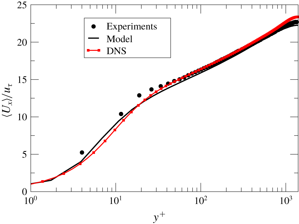
Mean velocity profiles. Comparison between experiments (points), DNS (squares–line) and the present model (solid line). All quantities are normalized in wall units.

4 Results
In figure 1, mean velocity profiles from experiments, DNS and model simulations are compared. The agreement of mean velocity is overall very good. Notably the model behaviour is analogous to that of the DNS, yet some small discrepancies can be detected in the viscous and buffer layers ( $4<y^{+}<50$), pointing to a small difference between experimental and numerical results. As highlighted by Stelzenmuller et al. (Reference Stelzenmuller, Polanco, Vignal, Vinkovic and Mordant2017), the first experimental points computed in the vicinity of the wall are affected by more important errors, due to experimental difficulties in the measurements. In particular, the position is measured with some amount of error.
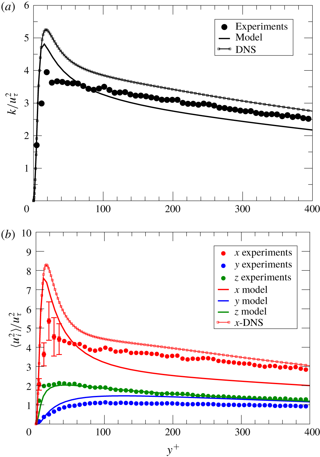
Comparison between experiments (points), DNS (squares–lines) and the present model (solid lines). All quantities are normalized in wall units. (a) Turbulent kinetic energy. (b) Reynolds-stress components.

In figure 2 the turbulent kinetic energy  $k$ is plotted (figure 2a), as well as each diagonal component of the Reynolds stress tensor (figure 2b). Given that we use a hybrid approach, all the Reynolds stresses are computed in the model by the RANS method. In the present model only the turbulent kinetic energy
 $k$ (i.e. the trace of the Reynolds stress tensor) is used in the Lagrangian stochastic model, so this is the key quantity for its performance. As shown in figure 2(a), the agreement among the three datasets is quite satisfactory. In particular, the model correctly represents the physics in the near-wall region, while it underestimates a little the turbulent energy far from the wall. Figure 2(b) shows that the Reynolds-stress model equipped with elliptical relaxation gives a satisfactory representation of each component of the Reynolds stress, notably in the near-wall region. A previous study (Pope Reference Pope2000) has shown that these RANS models tend nonetheless to underestimate the streamwise component in the log-layer region in very high-
 $Re$ flows, and that explains the slight discrepancy already noted for the turbulent energy for
 $y^{+}>200$ (see figure 2a). The model used is the best available among realisable RANS models for general wall-bounded flows (Pope Reference Pope2000), and the development of RANS models is not the focus of this work. Furthermore, as explained in § 3.1, it is more crucial to have consistency between the Eulerian and the Lagrangian models than to get perfect agreement with experiments at the level of mean fluid observables. The chosen model is therefore considered satisfactory with regard to the present purpose.
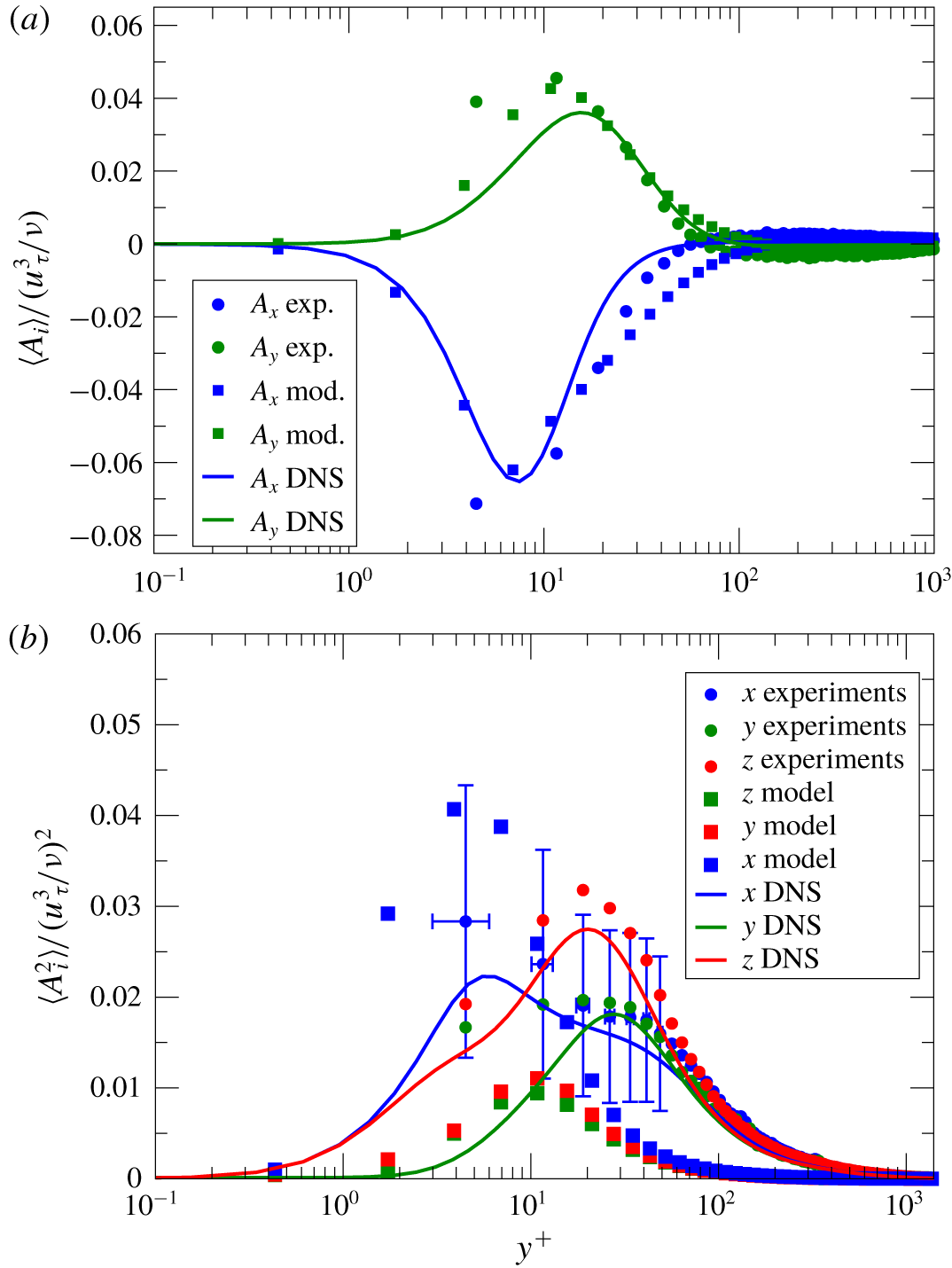
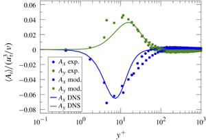
Mean (a) and variance (b) acceleration profiles. Comparison between experiments (points), stochastic model simulations (squares) and DNS (lines). Error bars are displayed for the  $x$ component of variance in experiments. As already remarked, the first experimental data are affected by large errors both in value and in position.

Figure 3 shows the acceleration mean and the acceleration variance profiles obtained from experiments, DNS and the model. The average acceleration is well predicted by the stochastic model in both directions. Notably the model gives correctly the negative peak of mean streamwise acceleration at  $y^{+}\approx 7$, which is a viscous effect. This shows that the acceleration model together with a RANS model including the boundary layer is able to describe this effect, despite the absence of ad hoc low-Reynolds-number terms in the stochastic model. It is also interesting to remark that the anisotropy between streamwise and wall-normal acceleration is correctly captured.
Profiles of acceleration variance (figure 3b) reveal a qualitative overall agreement, although larger discrepancies are found for the model concerning the acceleration variance. A slight overestimation of the streamwise variance is present with respect to DNS, even though the value found is within the experimental error bars. The other two components are instead slightly underestimated, notably the wall-normal component. Furthermore, the model displays a small degree of anisotropy between the  $y$ and
 $z$ components, both in amplitude and in the position of the peak, which is found at around the same position, whereas experiments and DNS show some variability. Yet at their respective peaks the standard deviation of the acceleration is larger than the magnitude of the mean acceleration for all sets, which is one of the salient characteristics of the acceleration process. This indicates that the present stochastic model is able to reproduce the main features of the acceleration fluctuations that govern the dynamics near the wall, although it fails to reproduce the anisotropy between the spanwise and the wall-normal components.
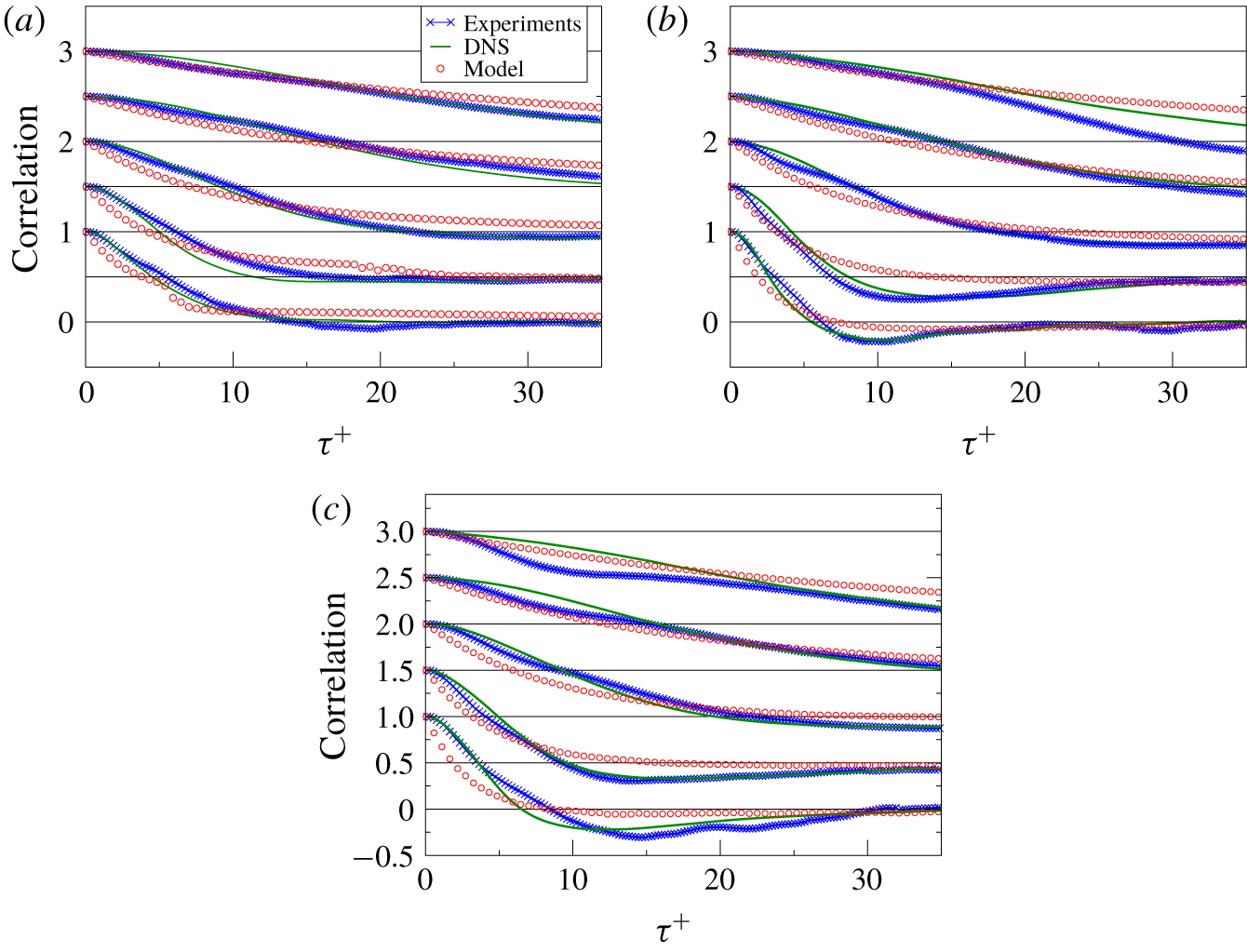
Lagrangian autocorrelations of (a) streamwise ( $\unicode[STIX]{x1D70C}_{xx}$), (b) wall-normal (
 $\unicode[STIX]{x1D70C}_{yy}$) and (c) spanwise (
 $\unicode[STIX]{x1D70C}_{zz}$) fluid particle acceleration. Experimental results are shown by blue lines with crosses, DNS results by solid green lines and model results by red circles. Curves are shifted vertically by increments of 0.5 for clarity. From bottom to top, the curves correspond to particles located initially at
 $y_{0}^{+}=20,60,200,600$ and 1000. Horizontal grid lines show the zero-correlation level for each
 $y_{0}^{+}$.

Figure 4 shows  $x,y$ and
 $z$ components of the acceleration correlation tensor
 $\unicode[STIX]{x1D70C}_{ij}$ calculated at different initial wall distances
 $y_{0}^{+}$. Correlations are computed as
 $$\begin{eqnarray}\unicode[STIX]{x1D70C}_{ij}(\unicode[STIX]{x1D70F},y_{0})=\frac{\langle A_{i}^{\prime }(t_{0},y_{0})A_{j}^{\prime }(t_{0}+\unicode[STIX]{x1D70F},y_{0})\rangle }{\langle A_{i}^{\prime 2}(t_{0},y_{0})\rangle ^{1/2}\langle A_{j}^{\prime 2}(t_{0}+\unicode[STIX]{x1D70F},y_{0})\rangle ^{1/2}},\end{eqnarray}$$
where  $A_{j}^{\prime }(t_{0}+\unicode[STIX]{x1D70F},y_{0})=A_{j}(t_{0}+\unicode[STIX]{x1D70F},y_{0})-\langle A_{j}(t_{0}+\unicode[STIX]{x1D70F},y_{0})\rangle$ is the fluid particle acceleration fluctuation relative to the Lagrangian average, with
 $i=x,y$ or
 $z$. The agreement is satisfactory, showing that the stochastic model fairly reproduces both the inhomogeneity and the anisotropy of the flow, since all components are different and the decorrelation time changes with the distance, as displayed by experiments and DNS. It is worth noting that the spanwise and wall-normal components as given by the stochastic model are a little more isotropic than the experimental results, yet more similar to DNS ones.
Some small differences for small time displacements, notably in the near-wall region, can be traced back to the presence of a white noise in the acceleration process which overlooks very short-memory effects. For long times, although the overall agreement remains fairly good, the stochastic model slightly overestimates the correlation time, so that acceleration appears to remain correlated over a longer time. This can be partially related to the choice of the coefficients of the model, and in particular we have chosen the time scale of the acceleration equal to  $\unicode[STIX]{x1D70F}_{\unicode[STIX]{x1D702}}$, while a coefficient of the order of, but different from, 1 might be used. Moreover, the statistical convergence of the correlations is particularly difficult and, therefore, a small residual bias error may be also present, for a finite number of particles have been used. The bias error is inherent to the stochastic models that include mean fields in the coefficients, whenever these coefficients are computed as averages over particles (Kloeden & Platen Reference Kloeden and Platen1992; Xu & Pope Reference Xu and Pope1999; Minier, Peirano & Chibbaro Reference Minier, Peirano and Chibbaro2003). This is precisely our case, as pointed out by formula (4.1).
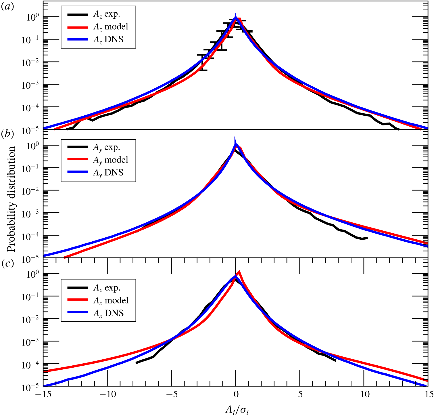
The PDFs of the (a) spanwise ( $z$), (b) wall-normal (
 $y$) and (c) streamwise (
 $x$) fluid particle acceleration. Experimental results are shown as solid black lines, DNS results as blue lines and model results as red lines. The PDFs are normalized by the root-mean-square value of acceleration (denoted
 $\unicode[STIX]{x1D70E}_{i}$ for each component) Reynolds number. The PDFs displayed represent an average over the whole channel in all cases. In experiments as well as in numerical simulations, we have released fluid parcels at different initial positions
 $y_{0}^{+}$, from
 $y_{0}^{+}=15$ to
 $y_{0}^{+}=1200$, every
 $y^{+}=10$. The global PDF is computed integrating the conditional statistics over
 $y_{0}$.

Figure 5 shows the PDFs of the three acceleration components. All curves present very long tails corresponding to extremely high acceleration events usually associated with intermittency (Mordant et al. Reference Mordant, Delour, Léveque, Arnéodo and Pinton2002). The model closely reproduces the experimental and DNS results. In particular, the model captures well the skewness of the acceleration, displaying a positive skewness for the wall-normal component and a negative skewness for the streamwise component. The spanwise component is correctly not skewed. The tails of the extreme events ( $P<10^{-4}$) appear slightly over-predicted by the model for the streamwise component. However, statistical error in this range is significant.
5 Discussion and conclusions
In this work, we have developed a novel stochastic model including fluid particle acceleration for general non-homogeneous turbulent flows, focusing on wall-bounded flows. This model generalises previous propositions of Lagrangian stochastic models for acceleration in isotropic flows, as well as the velocity-based models for non-homogeneous flows. Model results are compared against experimental and DNS measurements in a channel flow.
The Lagrangian stochastic model proposed has the structure of a diffusion process for the variables  $\boldsymbol{x},\boldsymbol{U},\boldsymbol{a}$, where
 $\boldsymbol{a}$ is a random acceleration process. The system appears as a set of SDEs, and it is closed using similarity arguments à la Kolmogorov and consistency with previous models in some limit cases. The coefficients of the resulting equations are functions of space and time, as well as being dependent on average fields. To find the fluid averages necessary for calculating the coefficients, we have used a hybrid RANS–PDF approach, typically used in realistic computations, where average velocity and Reynolds stress are computed in a Eulerian framework. In particular, we have chosen the elliptic-relaxation Reynolds-stress model to get a fair agreement between the RANS fields and the experimental ones.
The inclusion of acceleration in this stochastic model was motivated by the importance of this variable in the modelling of fast processes, which become especially important in the near-wall region. The results presented here are useful for disentangling to what extent the accurate modelling of the acceleration is important, and to what extent more complex closures are required.
The overall agreement between the model and experiments is good, showing that the present model captures most of the features revealed by experiments. In particular, the average acceleration is in very good agreement with experiments and DNS. The Lagrangian autocorrelation given by the model reproduces correctly the time scale and the non-homogeneous effects. These results are very encouraging for the modelling approach we have presented here, especially considering the relative simplicity of the model used for the acceleration variable, and that no free parameter has been calibrated.
The PDFs are also fairly well captured, displaying skewness, anisotropy and highly non-Gaussian tails. In homogeneous turbulence, the very wide tails of the acceleration PDF are associated with intermittency (Mordant et al. Reference Mordant, Metz, Michel and Pinton2001). In order to reproduce these features in stochastic models of homogeneous turbulence, a multiplicative component is added in the noise term to take into account the fluctuations of the dissipation rate  $\unicode[STIX]{x1D716}$ that are often assumed to follow log-normal statistics and to have a rather long correlation time close to
 $T_{L}$ (Pope & Chen Reference Pope and Chen1990; Mordant et al. Reference Mordant, Delour, Léveque, Arnéodo and Pinton2002; Reynolds Reference Reynolds2003a; Zamansky, Vinkovic & Gorokhovski Reference Zamansky, Vinkovic and Gorokhovski2010). Our model does not have such a multiplicative term in (2.5). However, the term
 $B$ incorporates the dissipation rate
 $\langle \unicode[STIX]{x1D716}\rangle$ which varies in space along the particle trajectory due to the inhomogeneity of the flow. It is thus a multiplicative term only related to inhomogeneity, and not with respect to the stochastic fluctuations of
 $\unicode[STIX]{x1D716}$. This contribution is enough to reproduce the wide-tail PDFs of the acceleration components. This confirms that in wall flows most of the extreme events are related to non-homogeneity (Lee, Yeo & Choi Reference Lee, Yeo and Choi2004). It also shows that the present model is able to capture the main statistical features of the near-wall structures that are responsible for the intermittency.
To further assess the acceleration model, we have also carried out simulations with the present stochastic model coupled with a simpler RANS model without the elliptical relaxation (see § 3). In this case, we assure consistency with the coefficients used in the velocity equation, but we lose the description of the near-wall region. For this reason, such a RANS model is much less accurate in wall flows; notably it is known to exaggerate the isotropy of the Reynolds stress, and to underestimate the kinetic energy (Pope Reference Pope2000). Interestingly, while the results obtained with this simpler model are inferior to those obtained with the complete model, the qualitative picture is similar and a fair agreement for all acceleration observables is still obtained. This shows robustness with respect to the RANS model used for the mean fields.
It is important to discuss now the deficiencies of the present model and to point out how to improve it.
(a) The anisotropy of the flow is not fully captured in the present framework. While anisotropy in mean acceleration and the PDF is correctly reproduced, acceleration variances in the spanwise and wall-normal directions turn out to be barely different, yet experiments and DNS show a more significant difference. Even if to a lesser extent, the same deficiency is found also looking at the correlations. This issue is mainly related to the modelling of the slow part of the fluctuating pressure gradient in the velocity equation (2.4), which is given in terms of the matrix  $\unicode[STIX]{x1D60E}_{ij}$. The simple Langevin model used here, equation (1.2) with
 $\unicode[STIX]{x1D60E}_{ij}^{a}=0$, is known to lead towards isotropy with respect to the two components (Pope Reference Pope2000). While the additional acceleration variable partially corrects this tendency, it is found to be insufficient to get a quantitative agreement. An elliptical-relaxation model should be implemented also in the Lagrangian stochastic model, as developed by Dreeben & Pope (Reference Dreeben and Pope1997). Furthermore, that would make the hybrid RANS–PDF approach more consistent, probably helping to recover a better level of the amplitude of the variances.
(b) The mean viscous term in the acceleration, equation (2.2), and the viscous transport term in the Reynolds-stress equations are neglected in the present approach, as displayed by (2.27). These terms are known to be very small except in a tiny region adjacent to walls (Pope Reference Pope2000). That is consistent with the fact the mean acceleration is so well reproduced by the present model. However, the viscous transport term would introduce explicitly the viscous time scale in the model and could help to further improve the prediction of the variances. Various models have been already proposed to include these terms (Dreeben & Pope Reference Dreeben and Pope1998; Wacławczyk, Pozorski & Minier Reference Wacławczyk, Pozorski and Minier2004).
(c) Although most of the intermittency is already captured, it would be possible to add also the internal intermittency due to the fluctuations of the turbulent dissipation (Pope Reference Pope2000; Lamorgese et al. Reference Lamorgese, Pope, Yeung and Sawford2007). Of course, these improvements bring a price in terms of computational and mathematical complexity.
In conclusion, despite some limitations, we believe that the present form of the stochastic model is adequate for modelling the acceleration dynamics in wall flows relevant for applications. As for general perspectives, concerning fluid flows, it would be interesting to pursue the analysis of conditional statistics for dispersion studies. Finally, the present model should be the starting point for developing an acceleration-based model for inertial particles.
Declaration of interests
The authors report no conflict of interest.