1 Introduction
The entropy wave generated in the flame zone of a combustor is a source of entropy noise and it can also affect combustion instability of the combustor. An accelerated entropy wave generates indirect noise and an entropy wave can also change the acoustic properties at the end of a combustor exit, becoming a source of combustion instability. A comprehensive review on this topic can be found in Morgans & Duran (Reference Morgans and Duran2016).
Polifke, Paschereit & Döbbeling (Reference Polifke, Paschereit and Döbbeling2001) reported that entropy waves can couple acoustic waves both constructively and destructively, and may significantly influence combustion stability. It was suggested that combustion stability analysis with a choked exit should consider the effects of entropy waves. Nicoud & Wieczorek (Reference Nicoud and Wieczorek2009) showed that the assumption of zero mean flow can lead to an erroneous prediction of combustion stability, as the zero mean flow is not able to accommodate entropy wave convection. Using a linearized Euler equation (LEE) model, Yu et al. (Reference Yu, Sisco, Sankaran and Anderson2010) numerically confirmed the location-dependent effects of an entropy wave on longitudinal combustion instability. Karimi, Brear & Moase (Reference Karimi, Brear and Moase2010) studied the interaction between sound waves and flows with steady heat communication and found that, at low frequencies, heat-induced entropy can generate sound comparable to the one caused by steady heat communication.
The dissipation and dispersion characteristics of an entropy wave after its generation at a flame zone has attracted much attention. Sattelmayer (Reference Sattelmayer2002) proposed a transfer function description of entropy wave dispersion due to combustor aerodynamics, and observed that the influence of an entropy wave on combustion stability can be overestimated unless the dispersion effect is appropriately compensated. Goh & Morgans (Reference Goh and Morgans2013) studied the effects of dissipation and dispersion of entropy waves on the stability of the combustor, and reported a combustor that can be driven to instability because of entropy waves. Fattahi, Hosseinalipour & Karimi (Reference Fattahi, Hosseinalipour and Karimi2017) showed that the high-frequency components of an entropy wave are easily attenuated and that the degree of low-frequency dissipation depends on turbulence intensity and thermal boundary conditions. An experimental study in Giusti et al. (Reference Giusti, Worth, Mastorakos and Dowling2017) revealed that the amplitude of entropy fluctuations decays as a function of wave parameters and propagation distance, and that the cause and extent of fluctuation decay can be well explained in terms of the local Helmholtz number. A simulation study in Morgans, Goh & Dahan (Reference Morgans, Goh and Dahan2013) suggested that entropy wave dissipation, predominantly caused by mean flow shear dispersion, can be negligible and consequently entropy-generated acoustic waves can be significant in combustion stability. Chen, Bomberg & Polifke (Reference Chen, Bomberg and Polifke2016) found that the assumption of an infinitesimally thin flame at rest can result in an incorrect prediction of entropy wave strength and, for a resolution, an interesting idea of a moving flame was proposed. Giusti, Magri & Zedda (Reference Giusti, Magri and Zedda2018) suggested that non-negligible fluctuations of temperature (entropy spots) and composition can reach a combustor exit, and that temperature fluctuations typically make stronger indirect noise than the compositional inhomogeneity. An experimental combustion instability believed to be a mixed entropy–acoustic mode was investigated by applying the dynamic mode decomposition technique to large-eddy simulation results in Motheau, Nicoud & Poinsot (Reference Motheau, Nicoud and Poinsot2014).
In spite of diverse research either emphasizing the importance of entropy waves in combustion stability study, or investigating the dissipation and dispersion of entropy waves inside a combustion chamber, surprisingly only a few studies in the literature have focused on entropy wave generation inside a flame zone with a non-zero thickness. A differential equation describing entropy wave transport was presented in Dowling (Reference Dowling1995), and its low- and high-frequency approximations were studied. In addition, Karimi, Brear & Moase (Reference Karimi, Brear and Moase2008) studied the spectral property of entropy waves from the perspective of disturbance energy for a model problem with a non-reflecting boundary condition. The concept of the ‘corner’ frequency, above which disturbance energy is dominated by acoustic disturbance, was introduced. This corner frequency, however, was implicitly defined as a root of a complicated algebraic equation, and hence it hardly allows physical interpretations in terms of system parameters.
It seems that the thin flame assumption and associated jump conditions are adopted in most theoretical studies of combustion stability in the literature. An inevitable consequence of assuming an infinitesimally thin flame, however, is that all wave dynamics inside a flame zone are totally ignored. This is typically harmless for acoustic waves, as they are sufficiently fast compared to a typical flame thickness. In contrast, an entropy wave can be arbitrarily slow and its behaviour inside a flame zone can matter to the overall acoustics of the combustor if the entropy wave significantly interacts with acoustic waves at a combustor outlet. A theoretical study on the generation of entropy waves inside a flame will be presented in this paper.
The properties of an entropy wave at the end of a flame zone should be known precisely, above all else, for the aforementioned study on entropy wave dissipation and dispersion to be practically useful. It will be shown in this paper that the strength of the entropy wave at the end of a flame zone depends heavily on the spatial distribution of flame fluctuations: a spatially concentrated flame gives rise to a stronger entropy wave with more high-frequency components in it, provided that all other system parameters are fixed. Since the thin flame hypothesis assumes an infinitesimally concentrated flame, a logical consequence is that the strength of the entropy wave obtained from the thin flame assumption is an extreme overestimation. This fact might be related to a possible overstatement of entropy wave dissipation and dispersion effects in a combustion chamber. Moreover, it suggests that one should be very cautious in characterizing the frequency dependence of entropy wave dissipation in a flame tube, for the entropy wave just after a flame zone itself depends significantly on the frequency.
We will also answer the fundamental question in this paper: What is a source of entropy waves? In other words, what physical conditions will result in no entropy waves? Heat inputs are responsible obviously, but this is not a satisfactory answer, since we know that a certain combination of non-zero heat inputs and acoustic fluctuations can also give no entropy waves. Dowling & Mahmoudi (Reference Dowling and Mahmoudi2015) claimed that the fluctuation of heat and mass flow rates is a source of entropy waves, which, however, is not generally true, as will be shown in this paper.
This paper is structured as follows. After a quick summary of a linearized Euler equation, a differential equation governing entropy wave generation is given and the source of entropy waves is identified in § 2.1. For a uniformly distributed steady/unsteady heat input, an analytic solution of the entropy transport equation is found in § 2.2. From that solution, we characterize key parameters and properties of entropy waves in § 2.3. We propose a temporal-spatial filtering interpretation of the entropy transport equation in § 2.4 for arbitrarily distributed flames. Our entropy models are compared to a popular model based on the jump conditions in § 2.5. After a numerical example illustrating our findings in § 3, a conclusion is given in § 4.
2 Entropy wave model
Let us start with notational conventions. As usual,  $\mathbb{R}$ and
 $\mathbb{C}$ denote the fields of real and complex numbers, respectively. For a time function
 $f(t)\in \mathbb{R}$ or a space–time function
 $g(x,t)\in \mathbb{R}$, we stick to the same function name but will use a new independent variable
 $s\in \mathbb{C}$ or
 $w\in \mathbb{R}$ to denote the Laplace or Fourier transform of that function. For example,
 $f(w)$ is the Fourier transform of
 $f(t)$ and
 $g(x,s)$ denotes the Laplace transform of
 $g(x,t)$. The letter
 $s\in \mathbb{C}$ is a complex variable but
 $\mathfrak{s}=\mathfrak{s}(x,t)$ denotes an entropy function. The symbol ‘
 $:=$’ means a definition. For a general space–time function
 $a(x,t)$, its steady and unsteady parts are denoted by
 $\overline{a}(x)$ and
 $a^{\prime }(x,t)$, respectively.
2.1 Linearized Euler equations
One-dimensional combustor model.

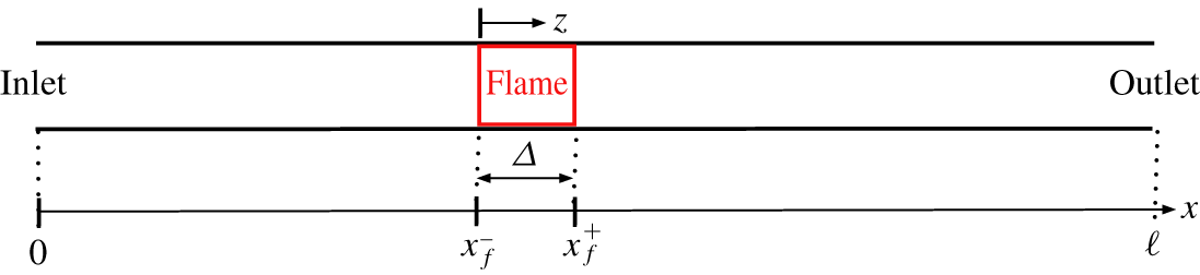
We consider a one-dimensional flow (left to right) through a duct of constant area  ${\mathcal{A}}\in \mathbb{R}$ and length
 $\ell \in \mathbb{R}$, along with heat communications over a compact interval
 $[x_{f}^{-},x_{f}^{+}]\subset [0,\ell ]$ as illustrated in figure 1.
The one-dimensional Euler equation is given
 $$\begin{eqnarray}\frac{\unicode[STIX]{x2202}}{\unicode[STIX]{x2202}x}\left[\begin{array}{@{}c@{}}\unicode[STIX]{x1D70C}u\\ p+\unicode[STIX]{x1D70C}u^{2}\\ \displaystyle \frac{\unicode[STIX]{x1D6FE}}{\unicode[STIX]{x1D6FE}-1}pu+\frac{1}{2}\unicode[STIX]{x1D70C}u^{3}\end{array}\right]+\frac{\unicode[STIX]{x2202}}{\unicode[STIX]{x2202}t}\left[\begin{array}{@{}c@{}}\unicode[STIX]{x1D70C}\\ \unicode[STIX]{x1D70C}u\\ \displaystyle \frac{p}{\unicode[STIX]{x1D6FE}-1}+\frac{1}{2}\unicode[STIX]{x1D70C}u^{2}\end{array}\right]=\left[\begin{array}{@{}c@{}}0\\ 0\\ 1\end{array}\right]q,\end{eqnarray}$$
with pressure  $p$, velocity
 $u$, density
 $\unicode[STIX]{x1D70C}$, heat rate input
 $q$ per unit volume, and
 $\unicode[STIX]{x1D6FE}:=c_{p}/c_{v}$, where
 $c_{p}$ and
 $c_{v}$ denote the heat capacity at constant pressure and volume, respectively.
Physical quantities  $\{p,u,\unicode[STIX]{x1D70C},q\}$ can be partitioned into their steady (mean) and unsteady (fluctuation) parts,
 $$\begin{eqnarray}\displaystyle p(x,t)=\overline{p}(x)+p^{\prime }(x,t),\quad u(x,t)=\overline{u}(x)+u^{\prime }(x,t), & & \displaystyle\end{eqnarray}$$
 $$\begin{eqnarray}\displaystyle \unicode[STIX]{x1D70C}(x,t)=\overline{\unicode[STIX]{x1D70C}}(x)+\unicode[STIX]{x1D70C}^{\prime }(x,t),\quad q(x,t)=\overline{q}(x)+q^{\prime }(x,t), & & \displaystyle\end{eqnarray}$$
and the Euler equation (2.1) can also be divided into its steady and unsteady parts neglecting nonlinear terms. The time-invariant steady part is
 $$\begin{eqnarray}\displaystyle & \displaystyle \unicode[STIX]{x1D642}\,\frac{\text{d}}{\text{d}x}\left[\begin{array}{@{}c@{}}\overline{p}\\ \overline{u}\\ \overline{\unicode[STIX]{x1D70C}}\end{array}\right]=\left[\begin{array}{@{}c@{}}0\\ 0\\ 1\end{array}\right]\overline{q}, & \displaystyle\end{eqnarray}$$
 $$\begin{eqnarray}\displaystyle & \displaystyle \unicode[STIX]{x1D642}:=\left[\begin{array}{@{}ccc@{}}0 & \overline{\unicode[STIX]{x1D70C}} & \overline{u}\\ 1 & 2\overline{\unicode[STIX]{x1D70C}}\,\overline{u} & \overline{u}^{2}\\ \displaystyle \frac{\unicode[STIX]{x1D6FE}}{\unicode[STIX]{x1D6FE}-1}\overline{u} & \displaystyle \frac{\unicode[STIX]{x1D6FE}}{\unicode[STIX]{x1D6FE}-1}\overline{p}+\frac{3}{2}\overline{\unicode[STIX]{x1D70C}}\,\overline{u}^{2} & \displaystyle \frac{1}{2}\overline{u}^{3}\end{array}\right], & \displaystyle\end{eqnarray}$$
and the matrix inversion  $\unicode[STIX]{x1D642}^{-1}$ gives a more explicit form:
 $$\begin{eqnarray}\frac{\text{d}}{\text{d}x}\left[\begin{array}{@{}c@{}}\overline{p}\\ \overline{u}\\ \overline{\unicode[STIX]{x1D70C}}\end{array}\right]=\frac{\unicode[STIX]{x1D6FE}-1}{\unicode[STIX]{x1D6FE}\overline{p}-\overline{\unicode[STIX]{x1D70C}}\overline{u}^{2}}\left[\begin{array}{@{}c@{}}-\overline{\unicode[STIX]{x1D70C}}\,\overline{u}\\ 1\\ -\overline{\unicode[STIX]{x1D70C}}/\overline{u}\end{array}\right]\overline{q}.\end{eqnarray}$$
The unsteady part is given as
 $$\begin{eqnarray}\displaystyle & \displaystyle \frac{\unicode[STIX]{x2202}}{\unicode[STIX]{x2202}x}\left(\unicode[STIX]{x1D642}\left[\begin{array}{@{}c@{}}p^{\prime }\\ u^{\prime }\\ \hat{\unicode[STIX]{x1D70C}}^{\prime }\end{array}\right]\right)+\unicode[STIX]{x1D641}\,\frac{\unicode[STIX]{x2202}}{\unicode[STIX]{x2202}t}\left[\begin{array}{@{}c@{}}p^{\prime }\\ u^{\prime }\\ \hat{\unicode[STIX]{x1D70C}}^{\prime }\end{array}\right]=\left[\begin{array}{@{}c@{}}0\\ 0\\ 1\end{array}\right]q^{\prime } & \displaystyle\end{eqnarray}$$
 $$\begin{eqnarray}\displaystyle & \displaystyle \unicode[STIX]{x1D641}:=\left[\begin{array}{@{}ccc@{}}0 & 0 & 1\\ 0 & \overline{\unicode[STIX]{x1D70C}} & \overline{u}\\ \displaystyle \frac{\unicode[STIX]{x1D6FE}}{\unicode[STIX]{x1D6FE}-1} & \overline{\unicode[STIX]{x1D70C}}\overline{u} & \displaystyle \frac{1}{2}\overline{u}^{2}\end{array}\right]. & \displaystyle\end{eqnarray}$$
By representing the component-wise matrix derivative  $\unicode[STIX]{x2202}\unicode[STIX]{x1D642}/\unicode[STIX]{x2202}x$ that appears in (2.7) as a linear function of the mean heat
 $\overline{q}$ from (2.6) and then applying the Laplace transform, we can obtain an unsteady dynamics
 $$\begin{eqnarray}\displaystyle \frac{\text{d}}{\text{d}x}\left[\begin{array}{@{}c@{}}p^{\prime }\\ u^{\prime }\\ \hat{\unicode[STIX]{x1D70C}}^{\prime }\end{array}\right] & = & \displaystyle \frac{s}{\unicode[STIX]{x1D6FE}\overline{p}-\overline{\unicode[STIX]{x1D70C}}\,\overline{u}^{2}}\left[\begin{array}{@{}ccc@{}}\overline{\unicode[STIX]{x1D70C}}\,\overline{u} & -\unicode[STIX]{x1D6FE}\overline{p}\,\overline{\unicode[STIX]{x1D70C}} & 0\\ -1 & \overline{\unicode[STIX]{x1D70C}}\,\overline{u} & 0\\ \overline{\unicode[STIX]{x1D70C}}/\overline{u} & -\overline{\unicode[STIX]{x1D70C}}^{2} & -(\unicode[STIX]{x1D6FE}\overline{p}-\overline{\unicode[STIX]{x1D70C}}\overline{u}^{2})/\overline{u}\end{array}\right]\left[\begin{array}{@{}c@{}}p^{\prime }\\ u^{\prime }\\ \hat{\unicode[STIX]{x1D70C}}^{\prime }\end{array}\right]\nonumber\\ \displaystyle & & \displaystyle +\,\frac{(\unicode[STIX]{x1D6FE}-1)}{\unicode[STIX]{x1D6FE}\overline{p}-\overline{\unicode[STIX]{x1D70C}}\,\overline{u}^{2}}\left[\begin{array}{@{}c@{}}-\overline{\unicode[STIX]{x1D70C}}\,\overline{u}\\ 1\\ -\overline{\unicode[STIX]{x1D70C}}/\overline{u}\end{array}\right]q^{\prime }(x,s)\nonumber\\ \displaystyle & & \displaystyle +\,\frac{(\unicode[STIX]{x1D6FE}-1)}{(\unicode[STIX]{x1D6FE}\overline{p}-\overline{\unicode[STIX]{x1D70C}}\,\overline{u}^{2})^{2}}\left[\begin{array}{@{}ccc@{}}\unicode[STIX]{x1D6FE}\overline{\unicode[STIX]{x1D70C}}\,\overline{u} & -\overline{\unicode[STIX]{x1D70C}}(\overline{\unicode[STIX]{x1D70C}}\,\overline{u}^{2}+\unicode[STIX]{x1D6FE}\overline{p}) & -\unicode[STIX]{x1D6FE}\overline{p}\,\overline{u}\\ -\unicode[STIX]{x1D6FE} & 2\overline{\unicode[STIX]{x1D70C}}\,\overline{u} & \overline{u}^{2}\\ \unicode[STIX]{x1D6FE}\overline{\unicode[STIX]{x1D70C}}/\overline{u} & \overline{\unicode[STIX]{x1D70C}}(\unicode[STIX]{x1D6FE}\overline{p}-3\overline{\unicode[STIX]{x1D70C}}\,\overline{u}^{2})/\overline{u}^{2} & -\unicode[STIX]{x1D6FE}\overline{p}/\overline{u}\end{array}\right]\left[\begin{array}{@{}c@{}}p^{\prime }\\ u^{\prime }\\ \hat{\unicode[STIX]{x1D70C}}^{\prime }\end{array}\right]\overline{q}(x),\quad\end{eqnarray}$$
with a zero temporal initial condition  $[p^{\prime }(x,0)~u^{\prime }(x,0)~\unicode[STIX]{x1D70C}^{\prime }(x,0)]=[0~0~0]$.
The steady dynamics (2.6) is associated with a given spatial initial condition  $[\overline{p}(0)~\overline{u}(0)~\overline{\unicode[STIX]{x1D70C}}(0)]$ and the unsteady dynamics (2.9) is subject to boundary conditions
 $$\begin{eqnarray}[b_{1}(s)b_{2}(s)]\left[\begin{array}{@{}c@{}}p^{\prime }(0,s)\\ u^{\prime }(0,s)\end{array}\right]=0,\quad [c_{1}(s)c_{2}(s)c_{3}(s)]\left[\begin{array}{@{}c@{}}p^{\prime }(x,\ell )\\ u^{\prime }(x,\ell )\\ \hat{\unicode[STIX]{x1D70C}}^{\prime }(x,\ell )\end{array}\right]=0\end{eqnarray}$$
for a given set of scalar transfer functions  $\{b_{1,2}(s),c_{1,2,3}(s)\}$.
The steady dynamics (2.6) is an initial value problem and can be easily solved with any numerical integration method. In contrast, the unsteady dynamics (2.9)–(2.10) is an ordinary boundary value problem for each  $s\in \mathbb{C}$.
A differentiation of the unsteady entropy relation  $\mathfrak{s}^{\prime }=c_{v}(p^{\prime }/\overline{p}-\unicode[STIX]{x1D6FE}\unicode[STIX]{x1D70C}^{\prime }/\overline{\unicode[STIX]{x1D70C}})$ gives
 $$\begin{eqnarray}\frac{1}{c_{v}}\frac{\unicode[STIX]{x2202}\mathfrak{s}^{\prime }}{\unicode[STIX]{x2202}x}=\left[\begin{array}{@{}ccc@{}}1/\overline{p} & 0 & -\unicode[STIX]{x1D6FE}/\overline{\unicode[STIX]{x1D70C}}\end{array}\right]\frac{\unicode[STIX]{x2202}}{\unicode[STIX]{x2202}x}\left[\begin{array}{@{}c@{}}p^{\prime }\\ u^{\prime }\\ \hat{\unicode[STIX]{x1D70C}}^{\prime }\end{array}\right]+\left[\begin{array}{@{}ccc@{}}-p^{\prime }/\overline{p}^{2} & 0 & \unicode[STIX]{x1D6FE}\unicode[STIX]{x1D70C}^{\prime }/\overline{\unicode[STIX]{x1D70C}}^{2}\end{array}\right]\frac{\text{d}}{\text{d}x}\left[\begin{array}{@{}c@{}}\overline{p}\\ \overline{u}\\ \overline{\unicode[STIX]{x1D70C}}\end{array}\right],\end{eqnarray}$$
which can be combined with (2.9) and (2.11) to yield
 $$\begin{eqnarray}\frac{1}{R}\left(\frac{\unicode[STIX]{x2202}\mathfrak{s}^{\prime }}{\unicode[STIX]{x2202}x}+\frac{1}{\overline{u}}\frac{\unicode[STIX]{x2202}\mathfrak{s}^{\prime }}{\unicode[STIX]{x2202}t}\right)=\frac{\overline{q}}{\overline{p}\overline{u}}\,\left(\frac{q^{\prime }}{\overline{q}}-\frac{p^{\prime }}{\overline{p}}-\frac{u^{\prime }}{\overline{u}}\right),\end{eqnarray}$$
where  $R:=c_{p}-c_{v}=c_{p}/\unicode[STIX]{x1D702}$ is the specific gas constant and
 $\unicode[STIX]{x1D702}:=\unicode[STIX]{x1D6FE}/(\unicode[STIX]{x1D6FE}-1)$.
By multiplying mean flow  $\overline{u}$ to both sides of (2.12), one can recover a familiar entropy transport equation written as a material derivative. However, the form (2.12) is advantageous in that it clearly shows a physical source of entropy waves. To be concrete, from an elementary identity
 $$\begin{eqnarray}\frac{\overline{q}}{\overline{p}\overline{u}}\,\left(\frac{q^{\prime }}{\overline{q}}-\frac{p^{\prime }}{\overline{p}}-\frac{u^{\prime }}{\overline{u}}\right)=\left(\frac{q}{pu}\right)^{\prime },\end{eqnarray}$$
the entropy equation (2.12) and the fact that
 $$\begin{eqnarray}\frac{q}{pu}=\frac{q{\mathcal{A}}}{pu{\mathcal{A}}}=\frac{\text{heat}\;\text{power}}{\text{flow}\;\text{power}},\end{eqnarray}$$
we discover that the fluctuation of the heat/flow power ratio (2.14) is the source of the entropy wave.
Consequently, no entropy wave is generated if and only if  $q=k\cdot pu$ holds for a constant
 $k\in \mathbb{R}$. A trivial condition
 $q=0$ for no entropy waves corresponds to the choice
 $k=0$.
If temperature  $T$ is constant, then we have
 $(q/pu)^{\prime }R\,\overline{T}=(q{\mathcal{A}}/{\dot{m}})^{\prime }$ with the mass flow rate
 ${\dot{m}}:=\unicode[STIX]{x1D70C}{\mathcal{A}}u$ from the ideal gas law. Conversely, for the condition
 $(q{\mathcal{A}}/{\dot{m}})^{\prime }=0$ to give
 $(q/pu)^{\prime }=0$, an equality
 $\unicode[STIX]{x1D70C}^{\prime }/\overline{\unicode[STIX]{x1D70C}}=p^{\prime }/\overline{p}$ should hold and this equality requires a constant
 $T$ from the ideal gas law. To sum up, the claim in Dowling & Mahmoudi (Reference Dowling and Mahmoudi2015) that the fluctuation of the heat/mass flow ratio generates the entropy wave is correct only when the temperature is constant.
2.2 Solution of entropy transport equation
The transfer function of an input–output pair of a general linear system is the Laplace transform of the impulse response, which is an output corresponding to an impulse input. Thus, for a transfer function representation of entropy wave, we need to solve the entropy transport equation (2.12) for given steady heat input  $\overline{q}(x)$ and normalized unsteady heat input
 $$\begin{eqnarray}q^{\prime }(x,t):=q_{x}^{\prime }(x)q_{t}^{\prime }(t),\quad \int _{0}^{\ell }q_{x}^{\prime }(x,t)\,\text{d}x=1,\end{eqnarray}$$
where  $q_{t}^{\prime }(t)=\unicode[STIX]{x1D6FF}(t)$ is the Dirac delta function. For a survey of transfer function approaches for partial differential equations, see Curtain & Morris (Reference Curtain and Morris2009).
It should be noted here that the pressure and velocity fluctuations  $p^{\prime }$ and
 $u^{\prime }$ on the right-hand side of the entropy transport equation (2.12) are solutions of the unsteady dynamics (2.9) with the same heat inputs and given boundary conditions.
In the following developments, even though  $q_{t}^{\prime }(s)=1$ as
 $q_{t}^{\prime }(t)=\unicode[STIX]{x1D6FF}(t)$, we will write
 $q_{t}^{\prime }(s)$ in order to express the dependence of the entropy wave on three fluctuations (heat
 $q^{\prime }$, pressure
 $p^{\prime }$ and velocity
 $v^{\prime }$) separately.
For an analytical solution of the entropy transport equation (2.12), we need some assumptions. Before proceeding, let us make a notational convention that every physical quantity before and after a flame zone will be represented by the two subscripts ‘1’ and ‘2’, respectively. For instances, mean flow before a flame is  $\overline{u}(x_{f}^{-}):=\overline{u}_{1}$ and pressure fluctuation at the end of a flame zone is written as
 $p^{\prime }(x_{f}^{+},t):=p_{2}^{\prime }(t)$.
We suppose that both steady and unsteady heat inputs have uniform distribution over an interval  $[x_{f}^{-},x_{f}^{+}]\subset [0,\ell ]$:
 $$\begin{eqnarray}\frac{\overline{q}(x)}{\overline{Q}_{m}}=q_{x}^{\prime }(x)=\left\{\begin{array}{@{}ll@{}}1/\unicode[STIX]{x1D6E5},\quad & x\in [x_{f}^{-},x_{f}^{+}],\\ 0,\quad & \text{elsewhere},\end{array}\right.\end{eqnarray}$$
where  $\unicode[STIX]{x1D6E5}:=x_{f}^{+}-x_{f}^{-}$ and
 $\overline{Q}_{m}:=\int _{x_{f}^{-}}^{x_{f}^{+}}\overline{q}(x)\,\text{d}x$.
In addition, we adopt the compact flame assumption that the flame thickness  $\unicode[STIX]{x1D6E5}$ is much shorter than the acoustic wavelengths under consideration. We also assume that the steady pressure is constant,
 $\overline{p}(x)=\overline{p}_{1}=\overline{p}_{2}$, and that the square of the mean flow Mach number can be neglected, that is,
 $\unicode[STIX]{x1D6FE}\overline{p}\gg \overline{\unicode[STIX]{x1D70C}}\overline{u}^{2}$ holds.
Under these assumptions, the steady energy conservation
 $$\begin{eqnarray}c_{p}\overline{\unicode[STIX]{x1D70C}}_{1}\overline{u}_{1}[\overline{T}_{2}-\overline{T}_{1}]=\int _{x_{f}^{-}}^{x_{f}^{+}}\overline{q}(x)\,\text{d}x=\overline{Q}_{m}\end{eqnarray}$$
across a flame, combined with the ideal gas law, gives
 $$\begin{eqnarray}\displaystyle \overline{Q}_{m}=c_{p}\overline{\unicode[STIX]{x1D70C}}_{1}\overline{u}_{1}\overline{T}_{1}(\unicode[STIX]{x1D6FC}-1)=\unicode[STIX]{x1D702}\overline{p}_{1}\overline{u}_{1}(\unicode[STIX]{x1D6FC}-1), & & \displaystyle\end{eqnarray}$$
where
 $$\begin{eqnarray}\unicode[STIX]{x1D6FC}=\unicode[STIX]{x1D6FC}(\overline{Q}_{m},\overline{u}_{1}):=\frac{\overline{T}_{2}}{\overline{T}_{1}}=\frac{\overline{Q}_{m}}{\unicode[STIX]{x1D702}\overline{p}_{1}\overline{u}_{1}}+1\end{eqnarray}$$
denotes the ratio of mean temperatures across a flame.
In addition, the assumption  $\unicode[STIX]{x1D6FE}\overline{p}\gg \overline{\unicode[STIX]{x1D70C}}\overline{u}^{2}$ allows us to easily find the mean flow from (2.6) as
 $$\begin{eqnarray}\overline{u}(x)-\overline{u}_{1}=\frac{1}{\unicode[STIX]{x1D702}\overline{p}_{1}}\int _{x_{f}^{-}}^{x}\overline{q}(x)\,\text{d}x=\frac{(\unicode[STIX]{x1D6FC}-1)\overline{u}_{1}}{\unicode[STIX]{x1D6E5}}\,(x-x_{f}^{-}),\end{eqnarray}$$
and thus  $\overline{u}_{2}=\unicode[STIX]{x1D6FC}\,\overline{u}_{1}$ holds. A combination of (2.20) and (2.19) yields
 $$\begin{eqnarray}\overline{u}_{2}\rightarrow \frac{\overline{Q}_{m}}{\unicode[STIX]{x1D702}\overline{p}_{1}}\quad \text{as }\overline{u}_{1}\rightarrow 0.\end{eqnarray}$$
This simple fact should be kept in mind in order to avoid confusion regarding the strength of the entropy wave under a zero mean flow condition, as will be discussed later.
We have a constant pressure and a known mean flow in (2.20) but the entropy transport equation (2.12) still includes two space-dependent unknown source terms  $\{p^{\prime },u^{\prime }\}$. This is a critical bottleneck in seeking an analytic solution, and a further approximation is needed. For this, it is first noted that
 $p^{\prime }(x,s)$ and
 $u^{\prime }(x,s)$ are continuous functions of the spatial variable
 $x$, being solutions of the differential equation (2.9). Secondly, we note that typical sinusoidal mode shapes of
 $p^{\prime }(x,\text{j}w^{\ast })$ and
 $u^{\prime }(x,\text{j}w^{\ast })$ at a low resonance frequency
 $w^{\ast }$ have only a couple of nodes in the full range
 $[0,\ell ]$ and vary smoothly overall. These two observations suggest that the variations of
 $p^{\prime }$ and
 $u^{\prime }$ over a compact interval
 $\unicode[STIX]{x1D6E5}\ll \ell$, i.e. a flame zone, will be small. In contrast to this, the entropy wave
 $s^{\prime }(x,\text{j}w)$ is fully generated inside the interval
 $\unicode[STIX]{x1D6E5}$ only. This rationale motivates us to adopt an approximation,
 $$\begin{eqnarray}p^{\prime }(x,t)\approx p_{1}^{\prime }(t)\approx p_{2}^{\prime }(t),\quad u^{\prime }(x,t)\approx u_{1}^{\prime }(t)\approx u_{2}^{\prime }(t),\end{eqnarray}$$
for all  $x\in [x_{f}^{-},x_{f}^{+}]$ in solving the entropy transport equation (2.12). For a quick intuition on the validity of such approximations, readers may look in advance at figures 10–12 where the shaded rectangle around
 $x=0.8$ represents the flame zone.
One might be concerned that the second approximation in (2.22) is incompatible with the famous velocity jump
 $$\begin{eqnarray}u^{\prime }(x_{f}^{+},s)-u^{\prime }(x_{f}^{-},s)=\frac{1}{\unicode[STIX]{x1D702}\overline{p}_{1}}q_{{\mathcal{A}}}^{\prime }(x_{f},s)\end{eqnarray}$$
across a thin flame  $\unicode[STIX]{x1D6E5}\approx 0$ with a heat rate input
 $q_{{\mathcal{A}}}^{\prime }$ per unit area under the zero mean flow condition (e.g. see (46) of Dowling & Stow (Reference Dowling and Stow2003)). One can also find numerical results in the literature where velocity mode shapes are far from sinusoidal, alluding to the approximation
 $u_{1}^{\prime }\approx u_{2}^{\prime }$ being unjustifiable (e.g. see figure 6 of Nicoud & Wieczorek (Reference Nicoud and Wieczorek2009) or figure 3 of Wieczorek et al. (Reference Wieczorek, Sensiau, Polifke and Nicoud2011)). A critical fact, however, is that, in those papers, an
 $n{-}\unicode[STIX]{x1D70F}$ flame transfer function
 $$\begin{eqnarray}\frac{q_{{\mathcal{A}}}^{\prime }(x_{f},s)}{u^{\prime }(x_{f}^{-},s)}=\frac{\overline{Q}_{m}}{\overline{u}_{1}}\,n\text{e}^{-\unicode[STIX]{x1D70F}s}\quad (n,\unicode[STIX]{x1D70F}\in \mathbb{R})\end{eqnarray}$$
was employed and hence, in reality, they observed behaviours of a closed-loop system composed of the LEE (2.9) and the feedback input (2.24). An unstable closed-loop system and the jump relation (2.23) gave large velocity jumps and non-sinusoidal mode shapes. In contrast, in this paper, we seek a solution (output) of the non-homogeneous LEE (an open-loop system) with a fixed driving term (input)  $q^{\prime }(x,t)=q_{x}^{\prime }(x)\unicode[STIX]{x1D6FF}(t)$ in (2.16). It cannot be overemphasized that the approximation (2.22) is for that particular input, not the feedback input (2.24).
Now a coordinate translation  $z:=x-x_{f}^{-}$ and (2.20) give
 $$\begin{eqnarray}\overline{u}(z)=\unicode[STIX]{x1D6FD}z+\overline{u}_{1},\quad \unicode[STIX]{x1D6FD}:=\frac{(\unicode[STIX]{x1D6FC}-1)\overline{u}_{1}}{\unicode[STIX]{x1D6E5}},\end{eqnarray}$$
and the Laplace transform of (2.12) with a time-initial condition  $\mathfrak{s}^{\prime }(z,0)=0$ gives a linear differential equation for entropy transport
 $$\begin{eqnarray}\frac{\text{d}\mathfrak{s}^{\prime }}{\text{d}z}+\frac{s}{\overline{u}(z)}\mathfrak{s}^{\prime }=\frac{A}{\overline{u}(z)}+\frac{B}{\overline{u}^{2}(z)},\end{eqnarray}$$
where
 $$\begin{eqnarray}A:=\frac{R}{\unicode[STIX]{x1D6E5}\overline{p}_{1}}q_{t}^{\prime }(s)-\frac{R\overline{Q}_{m}}{\unicode[STIX]{x1D6E5}\overline{p}_{1}^{2}}\,p_{1}^{\prime }(s),\quad B:=-\frac{R\,\overline{Q}_{m}}{\unicode[STIX]{x1D6E5}\overline{p}_{1}}\,u_{1}^{\prime }(s).\end{eqnarray}$$
We make use of the integral factor
 $$\begin{eqnarray}\displaystyle \unicode[STIX]{x1D713}(z):=\exp \left(\int _{0}^{z}\frac{s}{\unicode[STIX]{x1D6FD}z+\overline{u}_{1}}\,\text{d}z\right)=(\unicode[STIX]{x1D6FD}z/\overline{u}_{1}+1)^{s/\unicode[STIX]{x1D6FD}} & & \displaystyle\end{eqnarray}$$
of the differential equation (2.26) and apply a spatial initial condition  $\mathfrak{s}^{\prime }(z,s)=0$ for
 $z\leqslant 0$, to find
 $$\begin{eqnarray}\displaystyle \mathfrak{s}^{\prime }(z,s) & = & \displaystyle \frac{1}{\unicode[STIX]{x1D713}(z)}\int _{0}^{z}\unicode[STIX]{x1D713}(z)\left[\frac{A}{\overline{u}(z)}+\frac{B}{\overline{u}^{2}(z)}\right]\,\text{d}z=\frac{A}{s}[1-(\unicode[STIX]{x1D6FD}z/\overline{u}_{1}+1)^{-s/\unicode[STIX]{x1D6FD}}]\nonumber\\ \displaystyle & & \displaystyle +\,\frac{B}{\overline{u}_{1}(s-a)}[(\unicode[STIX]{x1D6FD}z/\overline{u}_{1}+1)^{-1}-(\unicode[STIX]{x1D6FD}z/\overline{u}_{1}+1)^{-s/\unicode[STIX]{x1D6FD}}].\end{eqnarray}$$
Substituting  $A$ and
 $B$ in (2.27) back into (2.29) and doing some algebraic rearrangements, we obtain the entropy wave at flame exit
 $z=\unicode[STIX]{x1D6E5}$ given by
 $$\begin{eqnarray}\frac{\mathfrak{s}_{2}^{\prime }(s)}{c_{p}}=\frac{1-\unicode[STIX]{x1D6FC}^{-s/\unicode[STIX]{x1D6FD}}}{(\unicode[STIX]{x1D6FC}-1)s/\unicode[STIX]{x1D6FD}}\,\frac{q_{t}^{\prime }(s)}{\unicode[STIX]{x1D702}\overline{p}_{1}\overline{u}_{1}}-\frac{1-\unicode[STIX]{x1D6FC}^{-s/\unicode[STIX]{x1D6FD}}}{s/\unicode[STIX]{x1D6FD}}\,\frac{p_{1}^{\prime }(s)}{\overline{p}_{1}}-\frac{1-\unicode[STIX]{x1D6FC}^{-(s/\unicode[STIX]{x1D6FD}-1)}}{\unicode[STIX]{x1D6FC}(s/\unicode[STIX]{x1D6FD}-1)}\,\frac{u_{1}^{\prime }(s)}{\overline{u}_{1}}.\end{eqnarray}$$
Note that the term ‘ $s/\unicode[STIX]{x1D6FD}$’ appears as a whole in this representation and hence
 $\unicode[STIX]{x1D6FD}$ serves as a scaling factor of the Laplace variable
 $s\in \mathbb{C}$, for a given set of space-independent fluctuations
 $\{q_{t}^{\prime }(s),p_{1}^{\prime }(s),u_{1}^{\prime }(s)\}$ at a flame.
After a flame zone  $x>x_{f}^{+}$, there being no heat, entropy fluctuation is a homogeneous solution of (2.12) given
 $$\begin{eqnarray}\mathfrak{s}^{\prime }(x,s)=\mathfrak{s}_{2}^{\prime }(s)\,\text{e}^{-((x-x_{f}^{+})/\overline{u}_{2})s}\end{eqnarray}$$
and its magnitude is constant  $|\mathfrak{s}_{2}^{\prime }(\text{j}w)|=|\mathfrak{s}^{\prime }(x,\text{j}w)|$ for all
 $x\geqslant x_{f}^{+}$.
2.3 Entropy transfer functions
Recall that, for given boundary conditions, the pressure and velocity fluctuations in the entropy wave representation (2.30) are determined by steady and unsteady heat inputs. Notwithstanding this fact, for generality, we will regard the heat, pressure and velocity fluctuations as independent sources of entropy waves, because assuming particular boundary conditions will fix dynamic interrelation among those fluctuations.
Let us rewrite (2.30) as
 $$\begin{eqnarray}\displaystyle \frac{\mathfrak{s}_{2}^{\prime }(s)}{c_{p}}=\unicode[STIX]{x1D719}_{h}(s)\frac{q_{t}^{\prime }(s)}{\unicode[STIX]{x1D702}\overline{p}_{1}\overline{u}_{1}}+\unicode[STIX]{x1D719}_{p}(s)\frac{p_{1}^{\prime }(s)}{\overline{p}_{1}}+\unicode[STIX]{x1D719}_{v}(s)\frac{u_{1}^{\prime }(s)}{\overline{u}_{1}}, & & \displaystyle\end{eqnarray}$$
 $$\begin{eqnarray}\displaystyle \unicode[STIX]{x1D719}_{h}:=\frac{1}{\unicode[STIX]{x1D6FC}-1}\,\frac{1-\unicode[STIX]{x1D6FC}^{-s/\unicode[STIX]{x1D6FD}}}{s/\unicode[STIX]{x1D6FD}},\quad \unicode[STIX]{x1D719}_{p}:=-\frac{1-\unicode[STIX]{x1D6FC}^{-s/\unicode[STIX]{x1D6FD}}}{s/\unicode[STIX]{x1D6FD}},\quad \unicode[STIX]{x1D719}_{v}:=-\frac{1}{\unicode[STIX]{x1D6FC}}\,\frac{1-\unicode[STIX]{x1D6FC}^{-(s/\unicode[STIX]{x1D6FD}-1)}}{s/\unicode[STIX]{x1D6FD}-1},\qquad \quad & & \displaystyle\end{eqnarray}$$
where the subscripts of  $\unicode[STIX]{x1D719}_{h,p,v}$ denote heat, pressure and velocity.
We will call the complex-valued functions  $\{\unicode[STIX]{x1D719}_{h,p,v}\}$ entropy transfer functions, as they represent transfer functions from the heat, pressure and velocity fluctuations to entropy fluctuation at the end of a flame zone.
First we consider the case of zero mean heat  $\overline{Q}_{m}=0$. For this, we take a limit
 $\unicode[STIX]{x1D6FC}\rightarrow 1$ in (2.33) to obtain
 $\unicode[STIX]{x1D719}_{h}(s)=1$,
 $\unicode[STIX]{x1D719}_{p}(s)=\unicode[STIX]{x1D719}_{v}(s)=0$ and
 $$\begin{eqnarray}\lim _{\overline{Q}_{m}\rightarrow 0}\mathfrak{s}_{2}^{\prime }(s)=\frac{c_{p}}{\unicode[STIX]{x1D702}\overline{p}_{1}\overline{u}_{1}}\,q_{t}^{\prime }(s)\end{eqnarray}$$
from (2.32), which shows that only heat fluctuation can generate an entropy wave in this case. This result is consistent with the observation that  $\overline{Q}_{m}=0$ makes both the pressure and velocity disturbances on the right-hand side of (2.12) disappear.
We note that every entropy transfer function given in the form (2.33) has a common pole and zero at either  $s=0$ or
 $s=\unicode[STIX]{x1D6FD}$ and, after a pole–zero cancellation, it becomes an entire function with no poles. The zeros of transfer functions
 $\{\unicode[STIX]{x1D719}_{h}(s),\unicode[STIX]{x1D719}_{p}(s)\}$ are the roots of the equation
 $\unicode[STIX]{x1D6FC}^{-s/\unicode[STIX]{x1D6FD}}=\text{e}^{-(s\ln \unicode[STIX]{x1D6FC})/\unicode[STIX]{x1D6FD}}=1$:
 $$\begin{eqnarray}\left\{s=\text{j}\frac{2\unicode[STIX]{x03C0}\unicode[STIX]{x1D6FD}}{\ln \unicode[STIX]{x1D6FC}}\ell ;~\ell =\pm 1,\pm 2,\ldots \right\}\end{eqnarray}$$
situated on the imaginary axis of  $\mathbb{C}$, and similarly the zeros of
 $\unicode[STIX]{x1D719}_{v}(s)$ are
 $$\begin{eqnarray}\left\{s=\unicode[STIX]{x1D6FD}+\text{j}\frac{2\unicode[STIX]{x03C0}\unicode[STIX]{x1D6FD}}{\ln \unicode[STIX]{x1D6FC}}\ell ;~\ell =\pm 1,\pm 2,\ldots \right\}.\end{eqnarray}$$
It is noted that the zeros in (2.35) and (2.36) share the same imaginary parts. However, the zeros of the velocity–entropy transfer  $\unicode[STIX]{x1D719}_{v}(s)$ in (2.36) have a positive real part
 $\unicode[STIX]{x1D6FD}>0$ when
 $\unicode[STIX]{x1D6FC}>1$ and thus
 $\unicode[STIX]{x1D719}_{v}(s)$ is a non-minimum phase transfer function.
It is a standard fact in control theory that a non-minimum phase transfer function is prone to feedback instability (e.g. see Morgans & Annaswamy (Reference Morgans and Annaswamy2008)). This fact and the non-minimum phase property of  $\unicode[STIX]{x1D719}_{v}(s)$ suggest an instability mechanism in which an entropy wave convected to the combustor exit makes a reflected velocity fluctuation upstream, constituting a feedback loop (e.g. see Goh & Morgans (Reference Goh and Morgans2013) and Nicoud & Wieczorek (Reference Nicoud and Wieczorek2009)). Under this scenario, we can conjecture from
 $\unicode[STIX]{x1D6FD}=(\unicode[STIX]{x1D6FC}-1)\overline{u}_{1}/\unicode[STIX]{x1D6E5}$ in (2.25) that both a thinner flame and a faster mean flow can provoke this sort of combustion instability.
Choosing  $s=\text{j}w$,
 $w\in \mathbb{R}$, and a temperature ratio
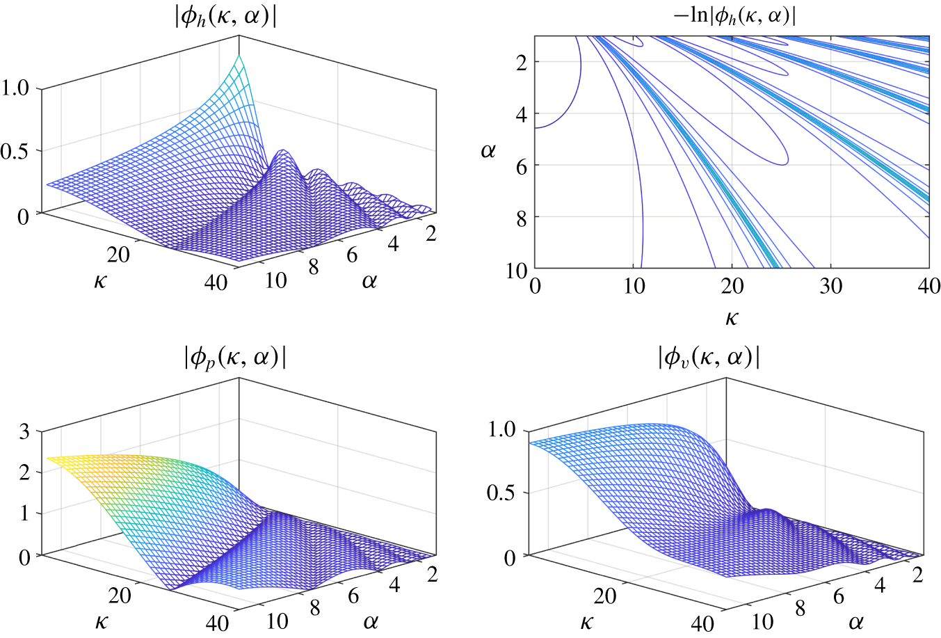
 $\unicode[STIX]{x1D6FC}\in [1,7]$ as two independent parameters, the magnitudes of entropy transfer functions
 $\{|\unicode[STIX]{x1D719}_{h,p,v}(s)|\}$ are shown in figure 2 with a normalized frequency
 $$\begin{eqnarray}\unicode[STIX]{x1D705}:=T_{p}\,w,\end{eqnarray}$$
where the quantity
 $$\begin{eqnarray}T_{p}:=\frac{\unicode[STIX]{x1D6E5}}{\,\overline{u}_{1}}=\frac{\unicode[STIX]{x1D6FC}-1}{\unicode[STIX]{x1D6FD}}\end{eqnarray}$$
denotes the flame passage time for the entropy wave to pass through the flame zone.
Magnitude of entropy transfer functions.

We can see a general dependence of entropy wave strength on temperature ratio and frequency in figure 2. The contour plot of  $-\ln |\unicode[STIX]{x1D719}_{h}(\unicode[STIX]{x1D705},\unicode[STIX]{x1D6FC})|$ in the upper-right corner highlights the set of pair
 $\{(\unicode[STIX]{x1D705},\unicode[STIX]{x1D6FC})\}$ for a small
 $|\unicode[STIX]{x1D719}_{h}(\unicode[STIX]{x1D705},\unicode[STIX]{x1D6FC})|$.
The overall decline of all magnitudes in figure 2 as the frequency  $\unicode[STIX]{x1D705}$ increases proves the low-pass filtering property of entropy waves. Another interesting observation is that a higher temperature ratio (equivalently, more steady heat) hinders heat fluctuation from generating an entropy wave. Contrariwise, it promotes entropy wave generation by both pressure and velocity fluctuations.
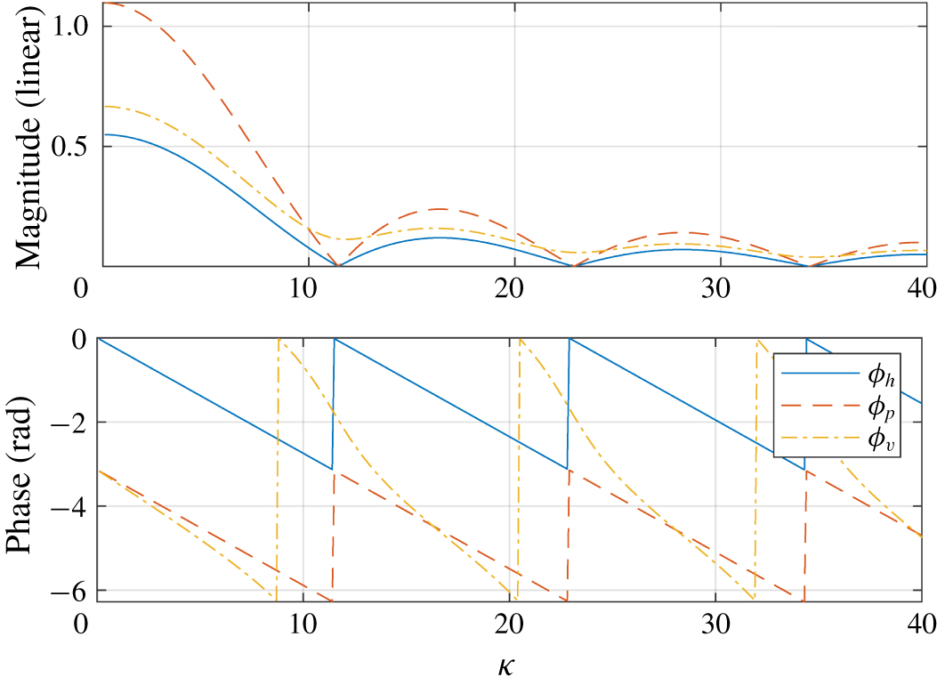
Being cross-sections of the plots in figure 2 at  $\unicode[STIX]{x1D6FC}=3$, the Bode (frequency response) magnitude plots of entropy transfer functions are shown in figure 3. Remarkably, the three transfer functions have local minima at the same frequencies and, in particular,
 $|\unicode[STIX]{x1D719}_{h}|=|\unicode[STIX]{x1D719}_{p}|=0$ holds at those frequencies.
Bode plot of entropy transfer functions ( $\unicode[STIX]{x1D6FC}=3$).

The pairs  $\{(\unicode[STIX]{x1D705},\unicode[STIX]{x1D6FC})\}$ giving a small magnitude, situated at the valleys in figure 2, and the set of frequencies achieving local minima of the Bode plot in figure 3 come from the zeros of transfer functions in (2.35) and (2.36) and thus such a pair
 $(\unicode[STIX]{x1D705},\unicode[STIX]{x1D6FC})$ satisfies
 $$\begin{eqnarray}\unicode[STIX]{x1D705}=\frac{2\unicode[STIX]{x03C0}(\unicode[STIX]{x1D6FC}-1)\ell }{\ln \unicode[STIX]{x1D6FC}}\quad (\ell =\pm 1,\pm 2,\ldots ).\end{eqnarray}$$
Therefore, when  $(\unicode[STIX]{x1D705},\unicode[STIX]{x1D6FC})$ satisfies (2.39), both the heat and pressure fluctuations do not contribute to entropy wave generation at all. In contrast, even in this case, the velocity fluctuation can generate weak waves.
Figure 2 and a choice of  $\ell =1$ in (2.39) give that the magnitude of the three entropy transfer functions decrease monotonically over a frequency range
 $[0,f_{c}]$ where
 $$\begin{eqnarray}f_{c}:=\left(\frac{\unicode[STIX]{x1D6FC}-1}{\ln \unicode[STIX]{x1D6FC}}\right)\frac{1}{T_{p}}=\left(\frac{\unicode[STIX]{x1D6FC}-1}{\ln \unicode[STIX]{x1D6FC}}\right)\frac{\,\overline{u}_{1}}{\unicode[STIX]{x1D6E5}}.\end{eqnarray}$$
We define  $f_{c}$ as the entropic cutoff frequency for presentational simplicity, against an engineering convention that a frequency achieving
 $-3~\text{dB}$ (70.7 %) attenuation is usually called the cutoff frequency.
One can see from (2.40) and (2.38) that either a thin flame or a fast mean flow makes a large  $f_{c}$ and thus a stronger entropy wave will occur downstream of a flame.
The dynamics of an entropy wave inside a flame zone can be safely ignored in an acoustic study of a combustor only when all entropy transfer functions can be approximated accurately as constants. For this, the cutoff frequency should be sufficiently higher than the maximal acoustic frequency in a particular acoustic study. A judgement on this point can be made from (2.40).
Now we will show that our cutoff frequency is a rigorous generalization of the corner frequency in Karimi et al. (Reference Karimi, Brear and Moase2008). The corner frequency, call it  $w_{n}\in \mathbb{R}$, was loosely defined as a frequency such that the ratio
 $|(\mathfrak{s}_{2}^{\prime }/u_{1}^{\prime })(\text{j}w_{n})|$ is small (recall that we assumed
 $u_{1}^{\prime }\approx u_{2}^{\prime }$) on the premise that there is no reflection at the end of the duct;
 $p_{2}^{\prime }=\overline{\unicode[STIX]{x1D70C}}_{2}\overline{c}_{2}u_{2}^{\prime }$ holds, where
 $\overline{c}_{2}$ denotes the sound speed after a flame.
Our entropy wave for this particular case can be written as
 $$\begin{eqnarray}\frac{\mathfrak{s}_{2}^{\prime }(s)}{c_{p}}=\unicode[STIX]{x1D719}_{h}(s)\frac{q_{t}^{\prime }(s)}{\unicode[STIX]{x1D702}\overline{p}_{1}\overline{u}_{1}}+[\unicode[STIX]{x1D6FE}\unicode[STIX]{x1D719}_{p}(s)/\overline{c}_{2}+\unicode[STIX]{x1D719}_{v}(s)/\overline{u}_{1}]\,u_{1}^{\prime }(s)\end{eqnarray}$$
from (2.32) and the facts  $\overline{p}_{1}=\overline{p}_{2}$ and
 $\unicode[STIX]{x1D6FE}\overline{p}_{2}=\overline{\unicode[STIX]{x1D70C}}_{2}\overline{c}_{2}^{2}$.
We have seen in (2.35) and (2.36) that the complex number  $s^{\ast }=\text{j}w_{c}$, where
 $w_{c}:=2\unicode[STIX]{x03C0}f_{c}\ell$ for any integer
 $\ell \in [1,\infty )$ is a zero of both
 $\unicode[STIX]{x1D719}_{h}(s)$ and
 $\unicode[STIX]{x1D719}_{p}(s)$ and, at the same time, it is a local minimum of
 $\unicode[STIX]{x1D719}_{v}(s)$ (recall figure 2 and figure 3). From this fact and the entropy form (2.41), it follows that
 $|(\mathfrak{s}_{2}^{\prime }/u_{1}^{\prime })(\text{j}w)|$ can be minimized by choosing
 $w=w_{c}=w_{n}$, where the second equality comes from the definition of the corner frequency. In short, the corner frequency of Karimi et al. (Reference Karimi, Brear and Moase2008) is a special case of our entropic cutoff frequency, associated with a reflectionless outlet.
Recall that our entropic cutoff frequency is completely determined by three system parameters, i.e. temperature ratio, mean flow and flame thickness, regardless of thermoacoustic relations among the heat, pressure and velocity fluctuations. This important fact seems to be unnoticed in Karimi et al. (Reference Karimi, Brear and Moase2008).
2.4 Temporal-spatial filtering approach
Up to now we have considered a uniformly distributed flame only. However, we have numerically found that, with other shapes of flame distributions such as Gaussian and triangular distributions, a thinner flame always gives rise to a stronger entropy wave. This section will show that such a tendency is an inherent nature of the entropy transport equation from a new temporal-spatial filtering interpretation.
In order to deal with a general flame distribution, we choose a constant approximation of mean flow,
 $$\begin{eqnarray}\overline{u}(x)\approx \frac{\overline{u}_{1}+\overline{u}_{2}}{2}=\left(\frac{\unicode[STIX]{x1D6FC}+1}{2}\right)\overline{u}_{1}:=\overline{u}_{m},\end{eqnarray}$$
inside a flame zone instead of the linear one in (2.25). This makes the entropy transport equation (2.12) have constant coefficients:
 $$\begin{eqnarray}\frac{\unicode[STIX]{x2202}\mathfrak{s}^{\prime }}{\unicode[STIX]{x2202}x}+\frac{1}{\overline{u}_{m}}\frac{\unicode[STIX]{x2202}\mathfrak{s}^{\prime }}{\unicode[STIX]{x2202}t}=n(x,t),\end{eqnarray}$$
where
 $$\begin{eqnarray}\displaystyle n(x,t):=\frac{R}{\overline{p}_{1}\overline{u}_{m}}\left[q_{x}^{\prime }(x)q_{t}^{\prime }(t)-\left(\frac{p^{\prime }(t)}{\overline{p}_{1}}+\frac{u^{\prime }(t)}{\overline{u}_{m}}\right)\overline{q}(x)\right]. & & \displaystyle\end{eqnarray}$$
The temporal-spatial (two-dimensional) Fourier transform of a real-valued space–time function  $f(x,t)\in \mathbb{R}$ is defined as a bijective mapping
 $$\begin{eqnarray}\displaystyle f(x,t)\quad \Longleftrightarrow \quad f(k,w):=\int _{-\infty }^{\infty }\int _{-\infty }^{\infty }f(x,t)\text{e}^{-\text{j}(kx+wt)}\,\text{d}x\,\text{d}t, & & \displaystyle\end{eqnarray}$$
where  $k\in \mathbb{R}$ and
 $w\in \mathbb{R}$ denote the wavenumber and frequency, respectively.
After extending the domain of the entropy function by defining  $s^{\prime }(x,t):=0$ for
 $x\in (-\infty ,0]$ harmlessly, we apply the temporal-spatial Fourier transform to both sides of (2.43) to obtain
 $$\begin{eqnarray}\frac{\mathfrak{s}^{\prime }(k,w)}{n(k,w)}=h(k,w),\end{eqnarray}$$
where the transfer function  $h(k,w)$ and the input
 $n(k,w)$ are given as
 $$\begin{eqnarray}\displaystyle & \displaystyle h(k,w):=\frac{1}{\text{j}(k+w/\overline{u}_{m})}, & \displaystyle\end{eqnarray}$$
 $$\begin{eqnarray}\displaystyle & \displaystyle n(k,w):=\frac{R}{\overline{p}_{1}\overline{u}_{m}}\left[q_{x}^{\prime }(k)q_{t}^{\prime }(w)-\left(\frac{p^{\prime }(w)}{\overline{p}_{1}}+\frac{u^{\prime }(w)}{\overline{u}_{m}}\right)\overline{q}(k)\right]. & \displaystyle\end{eqnarray}$$
A key interpretation of (2.46) is that the transfer function  $h(k,w)$ is a first-order low-pass filter with both the temporal variable
 $w\in \mathbb{R}$ and the spatial variable
 $k\in \mathbb{R}$. For a fixed spatial variable
 $k$, an entropy wave is an output of the temporal low-pass filter and, conversely, it can be seen as the output of a spatial low-pass filter when the temporal variable
 $w$ is fixed.
For a given input  $n(k,w)$, an entropy wave is the output of the filter
 $h(k,w)$ and thus its strength is a monotonically decreasing function of both the wavenumber
 $k$ and the temporal frequency
 $w$. The temporal low-pass filtering of an entropy wave has already been addressed before. Our focus here is that an entropy wave is an output of a spatial low-pass filter too and thus its strength depends on how much the input
 $n(k,w)$ includes high-wavenumber components in it. This fact and the following scaling relation of the Fourier transform,
 $$\begin{eqnarray}n(ax,t)\quad \Longleftrightarrow \quad \frac{1}{a}\,n(k/a,w)\quad (a>0),\end{eqnarray}$$
imply that the entropy wave will become stronger as the flame gets more localized in the spatial domain, i.e. when the flame gets thinner. To conclude, our spatial filtering interpretation of the entropy transport equation provides an elegant explanation for why a thinner flame will result in a stronger entropy wave, regardless of the flame distribution.
Arguably, the constant mean flow approximation in (2.42), which was technically essential for our filtering approach, is a crude one. Nevertheless, we will show that, in the case of a uniform distribution at least, the fundamental properties of an entropy wave obtained from the filtering approach are similar to those from the analytic approach in the previous section.
The uniform flame distribution gives
 $$\begin{eqnarray}\displaystyle n(k,w)=\frac{R}{\overline{p}_{1}\overline{u}_{m}}\left[q_{t}^{\prime }(w)-\left(\frac{p^{\prime }(w)}{\overline{p}_{1}}+\frac{u^{\prime }(w)}{\overline{u}_{m}}\right)\overline{Q}_{m}\right]\frac{1-\text{e}^{-\text{j}k\unicode[STIX]{x1D6E5}}}{\text{j}k\unicode[STIX]{x1D6E5}}, & & \displaystyle\end{eqnarray}$$
and thus from (2.46) and (2.19) the entropy wave becomes
 $$\begin{eqnarray}\displaystyle \frac{\overline{p}_{1}\overline{u}_{1}}{c_{p}}\,\mathfrak{s}^{\prime }(k,w) & = & \displaystyle \frac{1-\text{e}^{-\text{j}k\unicode[STIX]{x1D6E5}}}{\text{j}k\unicode[STIX]{x1D6E5}(\text{j}k+\text{j}w/\overline{u}_{m})}\frac{2}{(\unicode[STIX]{x1D6FC}+1)}\nonumber\\ \displaystyle & & \displaystyle \times \left[q_{t}^{\prime }(w)/\unicode[STIX]{x1D702}-(\unicode[STIX]{x1D6FC}-1)\left(\overline{u}_{1}\,p^{\prime }(w)+\frac{2\,\overline{p}_{1}}{\unicode[STIX]{x1D6FC}+1}u^{\prime }(w)\right)\right].\end{eqnarray}$$
An application of the inverse spatial Fourier transform gives
 $$\begin{eqnarray}\displaystyle \frac{\overline{p}_{1}\overline{u}_{1}}{c_{p}}\,\mathfrak{s}^{\prime }(x,w) & = & \displaystyle \frac{\overline{u}_{1}}{\text{j}w\unicode[STIX]{x1D6E5}}[(1-\text{e}^{-\text{j}wx/\overline{u}_{m}})\boldsymbol{u}(x)-(1-\text{e}^{-\text{j}w(x-\unicode[STIX]{x1D6E5})/\overline{u}_{m}})\boldsymbol{u}(x-\unicode[STIX]{x1D6E5})]\nonumber\\ \displaystyle & & \displaystyle \times \left[q_{t}^{\prime }(w)/\unicode[STIX]{x1D702}-(\unicode[STIX]{x1D6FC}-1)\left(\overline{u}_{1}\,p^{\prime }(w)+\frac{2\,\overline{p}_{1}}{(\unicode[STIX]{x1D6FC}+1)}u^{\prime }(w)\right)\right],\end{eqnarray}$$
where  $\boldsymbol{u}(x):=1$ if
 $x\geqslant 0$ and
 $\boldsymbol{u}(x):=0$ elsewhere. Consequently, the entropy wave at the end of the flame zone
 $x=x_{f}^{+}$ is given as
 $$\begin{eqnarray}\frac{\mathfrak{s}_{2}^{\prime }(w)}{c_{p}}=\unicode[STIX]{x1D713}_{h}(w)\frac{q_{t}^{\prime }(w)}{\unicode[STIX]{x1D702}\overline{p}_{1}\overline{u}_{1}}+\unicode[STIX]{x1D713}_{p}(w)\frac{p^{\prime }(w)}{\overline{p}_{1}}+\unicode[STIX]{x1D713}_{v}(w)\frac{u^{\prime }(w)}{\overline{u}_{1}},\end{eqnarray}$$
where
 $$\begin{eqnarray}\left.\begin{array}{@{}c@{}}\displaystyle \unicode[STIX]{x1D713}_{h}(w):=\frac{2}{\unicode[STIX]{x1D6FC}+1}\,\frac{1-\text{e}^{-\text{j}\unicode[STIX]{x1D707}w/\unicode[STIX]{x1D6FD}}}{\text{j}\unicode[STIX]{x1D707}w/\unicode[STIX]{x1D6FD}},\quad \unicode[STIX]{x1D713}_{p}(w):=-\frac{2(\unicode[STIX]{x1D6FC}-1)}{\unicode[STIX]{x1D6FC}+1}\,\frac{1-\text{e}^{-\text{j}\unicode[STIX]{x1D707}w/\unicode[STIX]{x1D6FD}}}{\text{j}\unicode[STIX]{x1D707}w/\unicode[STIX]{x1D6FD}},\\ \displaystyle \unicode[STIX]{x1D713}_{v}(w):=-\frac{4(\unicode[STIX]{x1D6FC}-1)}{(\unicode[STIX]{x1D6FC}+1)^{2}}\,\frac{1-\text{e}^{-\text{j}\unicode[STIX]{x1D707}w/\unicode[STIX]{x1D6FD}}}{\text{j}\unicode[STIX]{x1D707}w/\unicode[STIX]{x1D6FD}},\quad \unicode[STIX]{x1D707}:=2\frac{\unicode[STIX]{x1D6FC}-1}{\unicode[STIX]{x1D6FC}+1}.\end{array}\right\}\end{eqnarray}$$
Keeping the identity  $\unicode[STIX]{x1D6FC}^{-s/\unicode[STIX]{x1D6FD}}=\text{e}^{-(s\ln \unicode[STIX]{x1D6FC})/\unicode[STIX]{x1D6FD}}$ in mind and choosing
 $s=\text{j}w$, one can compare the heat/pressure entropy transfer functions in (2.54) with those in (2.33) of the previous section to find that the parameter
 $\unicode[STIX]{x1D707}=2(\unicode[STIX]{x1D6FC}-1)/(\unicode[STIX]{x1D6FC}+1)$ in (2.54) serves as a substitute for the quantity ‘
 $\ln \unicode[STIX]{x1D6FC}$’ that appeared implicitly in (2.33).
Bode magnitude plots of entropy transfer functions:  $\unicode[STIX]{x1D6FC}=2$ (a) and
 $\unicode[STIX]{x1D6FC}=4$ (b).

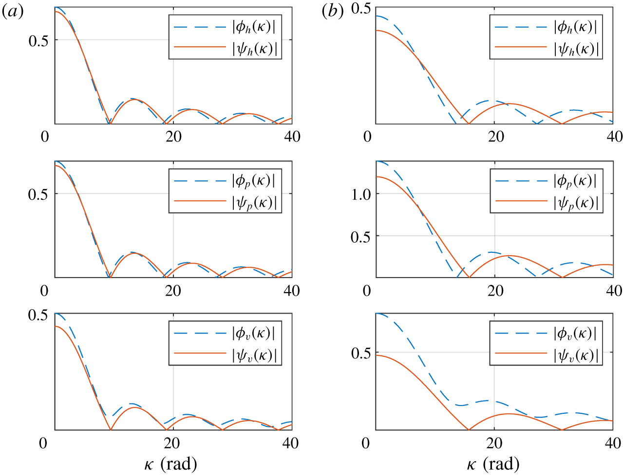
The frequency response of entropy transfer functions from the filtering approach in (2.54) and those from the analytic approach in (2.33) are compared in figure 4. To save space, only magnitudes with temperature ratios  $\unicode[STIX]{x1D6FC}\in \{2,4\}$ are shown. The case
 $\unicode[STIX]{x1D6FC}=2$ in figure 4(a) shows that the two groups of entropy transfer functions are surprisingly close to each other. The similarity gets weaker with
 $\unicode[STIX]{x1D6FC}=4$ in figure 4(b) but the overall shapes and magnitudes are still comparable.
The structural difference between the two velocity–entropy transfer functions in (2.54) and (2.33) even after the replacement of  $\unicode[STIX]{x1D707}$ with
 $\ln \unicode[STIX]{x1D6FC}$, and the numerical mismatch evident in figure 4 with
 $\unicode[STIX]{x1D6FC}=4$, seem to be consequences of the constant approximation of mean flow in (2.42).
2.5 Thin flame limit
When a flame is infinitesimally thin, entropy waves lose their dependence on the spatial domain and become static functions independent of frequency.
Since  $\unicode[STIX]{x1D705}=w\unicode[STIX]{x1D6E5}/\overline{u}_{1}=(\unicode[STIX]{x1D6FC}-1)w/\unicode[STIX]{x1D6FD}$, either
 $\unicode[STIX]{x1D6E5}\rightarrow 0$ or
 $w\rightarrow 0$ gives the same limit
 $\unicode[STIX]{x1D705}\rightarrow 0$. This fact and the dependence of entropy transfer functions (2.32) on the term
 $w/\unicode[STIX]{x1D6FD}$ give that the thin flame limit of our entropy wave solution is the same as its low-frequency limit. To be concrete, by taking the limit
 $\unicode[STIX]{x1D6FD}\rightarrow \infty$ in (2.33), we obtain the following thin flame limit or the low-frequency limit of the entropy wave:
 $$\begin{eqnarray}\lim _{\unicode[STIX]{x1D6E5}\rightarrow 0}\left[\frac{\overline{p}_{1}\overline{u}_{1}}{c_{p}}\,\mathfrak{s}_{2}^{\prime }(s)\right]=\frac{\ln \unicode[STIX]{x1D6FC}}{\unicode[STIX]{x1D702}(\unicode[STIX]{x1D6FC}-1)}\,q_{t}^{\prime }(s)-\ln \unicode[STIX]{x1D6FC}\cdot \overline{u}_{1}\,p_{1}^{\prime }(s)-\frac{\unicode[STIX]{x1D6FC}-1}{\unicode[STIX]{x1D6FC}}\,\overline{p}_{1}\,u_{1}^{\prime }(s).\end{eqnarray}$$
Now suppose further that the mean flow approaches zero, i.e.  $\overline{u}_{1}\rightarrow 0$, on top of the thin flame limit
 $\unicode[STIX]{x1D6E5}\rightarrow 0$. Then, from (2.19) and (2.21), we have
 $\ln \unicode[STIX]{x1D6FC}\cdot \overline{u}_{1}=(\ln \unicode[STIX]{x1D6FC}/\unicode[STIX]{x1D6FC})\overline{u}_{2}\rightarrow 0$ as
 $\overline{u}_{1}\rightarrow 0$. This fact and (2.55) give
 $$\begin{eqnarray}\lim _{\overline{u}_{1},\unicode[STIX]{x1D6E5}\rightarrow 0}[\overline{u}_{1}\,\mathfrak{s}_{2}^{\prime }(s)]=-c_{p}\,u_{1}^{\prime }(s),\end{eqnarray}$$
which means that only velocity fluctuation can generate an entropy wave in this case and that the strength of the entropy wave increases unboundedly as  $\overline{u}_{1}\rightarrow 0$.
The unboundedness of entropy strength with a zero mean flow has already been reported in the literature, including Dowling (Reference Dowling1995) and Dowling & Stow (Reference Dowling and Stow2003). However, the claim that  $\overline{u}_{2}\mathfrak{s}_{2}^{\prime }(s)$ is bounded as
 $\overline{u}_{2}\rightarrow 0$ in those papers is misleading and requires clarification in our view. First of all, we recall (2.21) that the limit
 $\overline{u}_{2}\rightarrow 0$ is not a correct description of the physical situation of zero mean flow
 $\overline{u}_{1}\rightarrow 0$. Moreover, by multiplying
 $\unicode[STIX]{x1D6FC}$ to both sides of (2.55) and setting
 $\overline{u}_{2}=\unicode[STIX]{x1D6FC}\overline{u}_{1}$, we obtain
 $$\begin{eqnarray}\lim _{\unicode[STIX]{x1D6E5}\rightarrow 0}\left[\frac{\overline{p}_{1}\overline{u}_{2}}{c_{p}}\,\mathfrak{s}_{2}^{\prime }(s)\right]=\frac{\unicode[STIX]{x1D6FC}\ln \unicode[STIX]{x1D6FC}}{\unicode[STIX]{x1D702}(\unicode[STIX]{x1D6FC}-1)}\,q_{t}^{\prime }(s)-\ln \unicode[STIX]{x1D6FC}\cdot \overline{u}_{2}\,p_{1}^{\prime }(s)-(\unicode[STIX]{x1D6FC}-1)\,\overline{p}_{1}\,u_{1}^{\prime }(s),\end{eqnarray}$$
where the three transfer functions on the right-hand side become unbounded as  $\unicode[STIX]{x1D6FC}\rightarrow \infty$, disputing the boundedness of
 $\overline{u}_{2}\mathfrak{s}_{2}^{\prime }(s)$.
A resolution comes from an observation that the limit  $\overline{u}_{1}\rightarrow 0$ with a fixed non-zero
 $\overline{Q}_{m}\neq 0$ is unrealistic since then the temperature after a flame increases unboundedly. A more practical situation is when both
 $\overline{u}_{1}\rightarrow 0$ and
 $\overline{Q}_{m}\rightarrow 0$ hold simultaneously in such a way as to keep a fixed temperature ratio
 $\unicode[STIX]{x1D6FC}$. The entropy wave in this case is given from (2.55) setting
 $\overline{u}_{1}=0$,
 $$\begin{eqnarray}\lim _{\overline{u}_{1},\unicode[STIX]{x1D6E5}\rightarrow 0}[\overline{u}_{1}\,\mathfrak{s}_{2}^{\prime }(s)]=\frac{R\ln \unicode[STIX]{x1D6FC}}{(\unicode[STIX]{x1D6FC}-1)\overline{p}_{1}}\,q_{t}^{\prime }(s)-c_{p}\frac{\unicode[STIX]{x1D6FC}-1}{\unicode[STIX]{x1D6FC}}\,u_{1}^{\prime }(s),\end{eqnarray}$$
which is valid only if the equality  $\overline{Q}_{m}=\unicode[STIX]{x1D702}\overline{p}_{1}(\unicode[STIX]{x1D6FC}-1)\overline{u}_{1}$ keeps holding during the limiting process
 $\overline{u}_{1}\rightarrow 0$. The boundedness of
 $\lim _{\overline{u}_{1}\rightarrow 0}\overline{u}_{2}\mathfrak{s}_{2}^{\prime }(s)=\unicode[STIX]{x1D6FC}\lim _{\overline{u}_{1}\rightarrow 0}\overline{u}_{1}\mathfrak{s}_{2}^{\prime }(s)$ now follows from (2.58) as
 $\unicode[STIX]{x1D6FC}$ therein is now a fixed constant by construction.
Under the assumption of an infinitesimally thin flame, the so-called jump conditions give an entropy model
 $$\begin{eqnarray}\frac{\overline{p}_{1}\overline{u}_{1}}{c_{p}}\,\mathfrak{s}_{2}^{\prime }(s)=\frac{1}{\unicode[STIX]{x1D702}\unicode[STIX]{x1D6FC}}\,q_{t}^{\prime }(s)-\frac{\unicode[STIX]{x1D6FC}-1}{\unicode[STIX]{x1D6FC}}\,\overline{u}_{1}\,p_{1}^{\prime }(s)-\frac{\unicode[STIX]{x1D6FC}-1}{\unicode[STIX]{x1D6FC}}\,\overline{p}_{1}\,u_{1}^{\prime }(s)\end{eqnarray}$$
after neglecting nonlinear terms (e.g. see equation (122) of Li et al. (Reference Li, Yang, Luzzato and Morgans2017)).
We first note that the zero mean flow limit (2.56) can also be obtained from (2.59) by taking the two limits  $\overline{u}_{1}\rightarrow 0$ and
 $\unicode[STIX]{x1D6FC}\rightarrow \infty$ simultaneously. Secondly, from a comparison of (2.59) with (2.55), we find a somewhat unexpected fact that the jump condition model is not identical to the thin flame limit of our model.
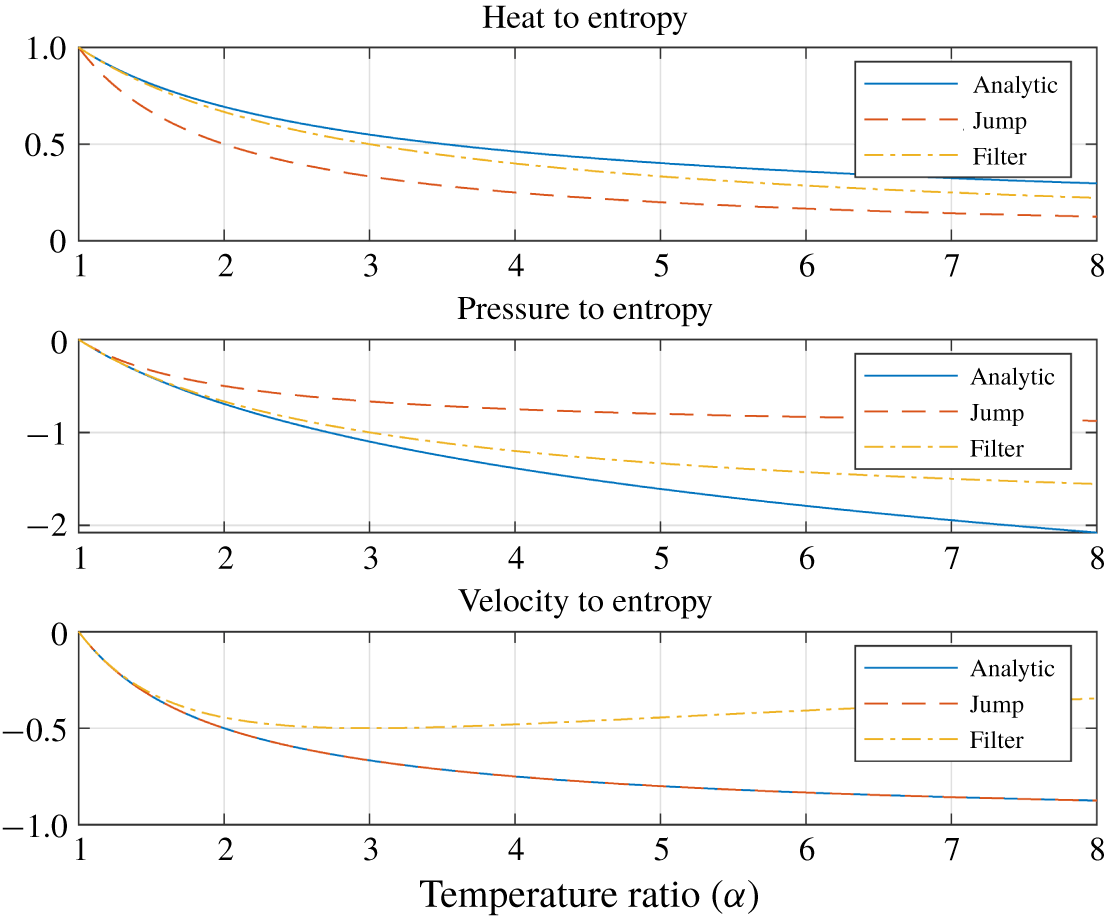
Figure 5 compares three groups of entropy transfer functions: the thin flame limit of our model in (2.55), the jump condition model (2.59) and the thin flame limit of the filter model (2.54) given by
 $$\begin{eqnarray}\frac{\overline{p}_{1}\overline{u}_{1}}{c_{p}}\mathfrak{s}_{2}^{\prime }(\text{j}w)=\frac{2}{\unicode[STIX]{x1D702}(\unicode[STIX]{x1D6FC}+1)}q_{t}^{\prime }(\text{j}w)-\frac{2(\unicode[STIX]{x1D6FC}-1)}{\unicode[STIX]{x1D6FC}+1}\overline{u}_{1}p_{1}^{\prime }(\text{j}w)-\frac{4(\unicode[STIX]{x1D6FC}-1)}{(\unicode[STIX]{x1D6FC}+1)^{2}}\overline{p}_{1}u_{1}^{\prime }(\text{j}w).\end{eqnarray}$$
Comparison of entropy transfer functions for a thin flame.

In addition to the overall similarity among the three groups of entropy transfer functions in figure 5, we can also see that, compared to the jump condition model, the analytic model and the filter model are closer to each other when it comes to the heat–entropy and pressure–entropy transfer functions. In contrast, in the case of the velocity–entropy transfer function, the filter model significantly deviates from the other two identical models, presumably due to the rough constant approximation in (2.42).
It is also noticeable that, compared to the thin flame limit of the analytic model, the jump condition model overestimates and underestimates the magnitudes of the pressure–entropy and heat–entropy transfer functions, respectively.
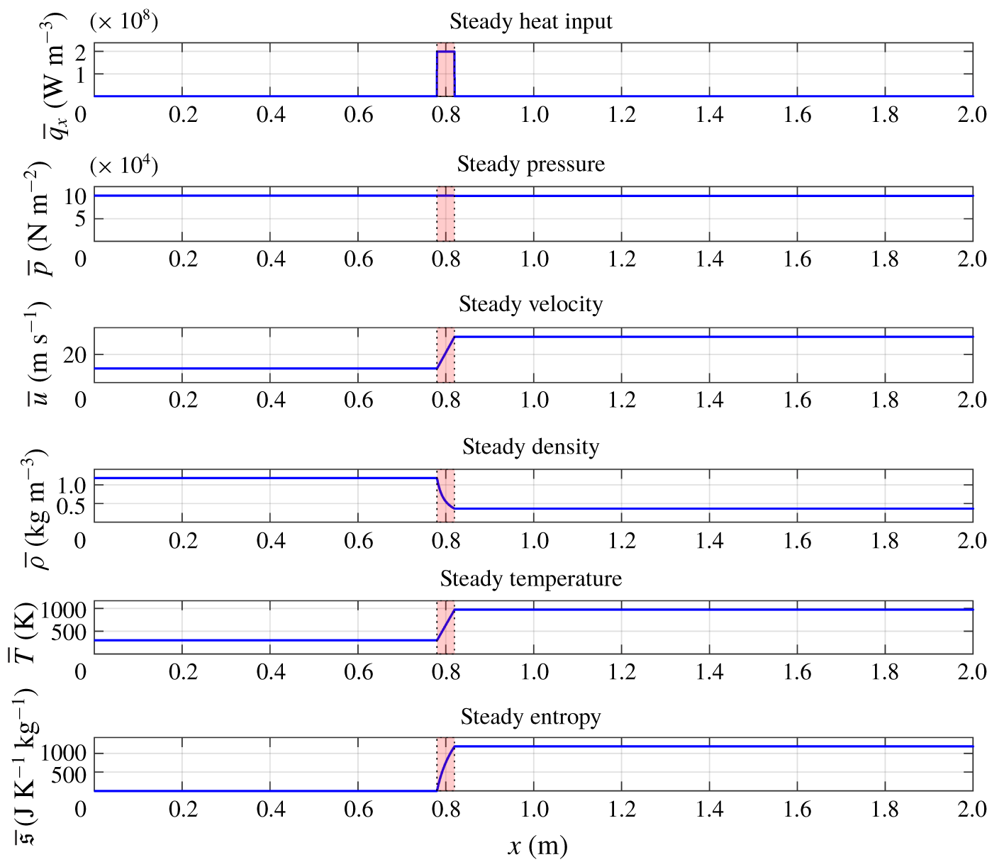
Steady properties.

3 An illustrative example
This section presents a numerical example substantiating our theoretical findings.
Consider air flows in a circular duct of radius 0.02 m and length 2.0 m in figure 1, with inlet parameters of pressure  $\overline{p}_{1}=10^{5}~\text{N}~\text{m}^{-2}$, temperature
 $\overline{T}_{1}=300~\text{K}$, mean flow
 $\overline{u}_{1}=10~\text{m}~\text{s}^{-1}$ and
 $\unicode[STIX]{x1D6FE}=1.4$, subject to the open–closed boundary conditions:
 $$\begin{eqnarray}p^{\prime }(0,t)=0,\quad u^{\prime }(\ell ,t)=0\quad (t\geqslant 0).\end{eqnarray}$$
We assumed a flame uniformly distributed with a centre  $(x_{f}^{+}+x_{f}^{-})/2=0.8~\text{m}$, thickness
 $\unicode[STIX]{x1D6E5}=0.04~\text{m}$ and steady heat release rate
 $\overline{Q}_{m}=10^{4}~\text{W}~\text{m}^{-2}$.
By solving (2.6), the mean physical quantities after the flame were found to be  $\overline{p}_{2}=1.01\times 10^{5}$,
 $\overline{u}_{2}=32.5$,
 $\overline{T}_{2}=973$ and
 $\unicode[STIX]{x1D6FC}=3.244$. The spatial distribution of steady heat input, pressure, velocity, density, temperature and entropy are shown in figure 6, where the shaded rectangle around
 $x=0.8$ indicates the flame zone.
The solutions of the Euler equation (2.9), which is a distributed transfer function from the heat fluctuation to the acoustic and entropic fluctuations, were computed using the function bvp4c.m of the software MATLAB© with  $10^{4}$ spatial grids and
 $600$ frequency points in the interval
 $[1,600]~\text{Hz}$. The computation time depended slightly on the particular flame thickness and heat distribution shapes, but typically it took only a couple of minutes with a standard desktop computer.
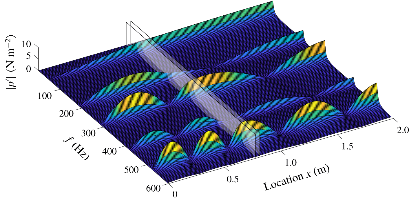
Magnitude of pressure wave  $|p^{\prime }(x,\text{j}2\unicode[STIX]{x03C0}f)|$.

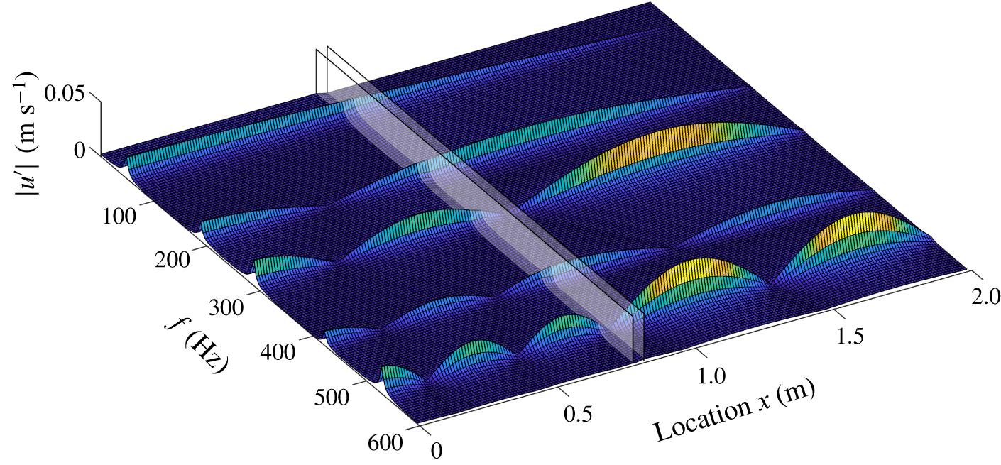
Magnitude of velocity wave  $|u^{\prime }(x,\text{j}2\unicode[STIX]{x03C0}f)|$.

Magnitude of entropy wave  $|\mathfrak{s}^{\prime }(x,\text{j}2\unicode[STIX]{x03C0}f)|$.

Pressure mode shape  $|p^{\prime }(x,\text{j}2\unicode[STIX]{x03C0}f)|$.

Velocity mode shape  $|u^{\prime }(x,\text{j}2\unicode[STIX]{x03C0}f)|$.

Entropy mode shape  $|\mathfrak{s}^{\prime }(x,\text{j}2\unicode[STIX]{x03C0}f)|$.

Entropy magnitudes at resonance frequency.

Entropy magnitude with normalized frequency.

Bode (magnitude) plot of entropy wave.

Entropy energy versus flame thickness.

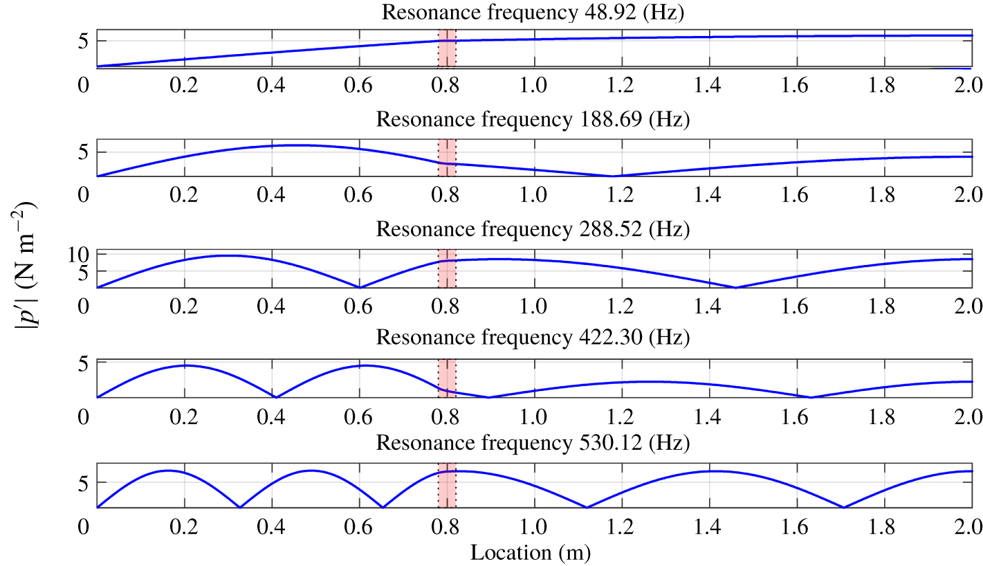
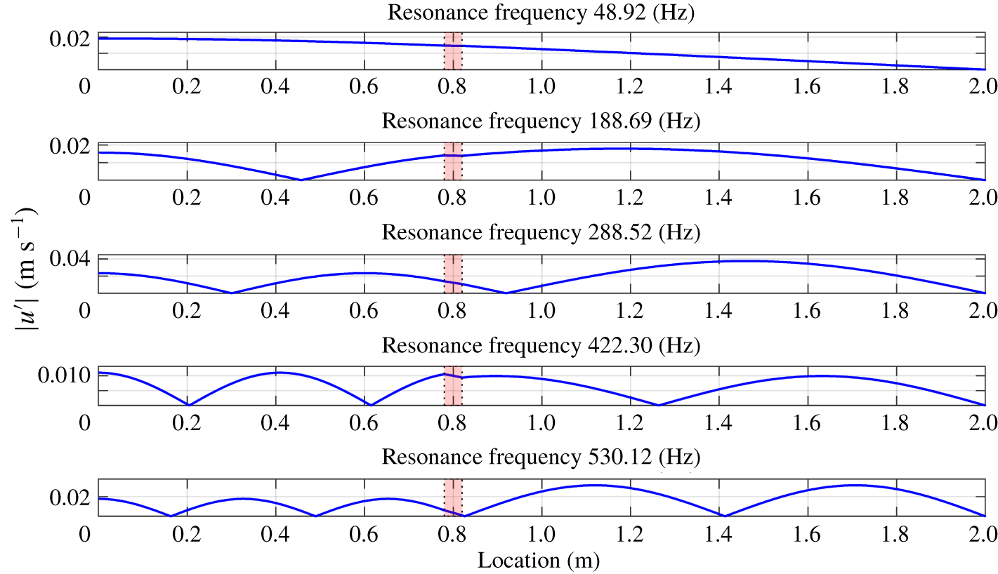
The magnitudes of pressure and velocity fluctuations are, respectively, shown in figure 7 and figure 8, in which the two shaded rectangle planes indicate the start and end of a flame zone. Both figures clearly show five resonance frequencies (Hz)
 $$\begin{eqnarray}\{48.92,~188.69,~288.52,~422.30,~530.12\}\end{eqnarray}$$
and corresponding mode shapes simultaneously.
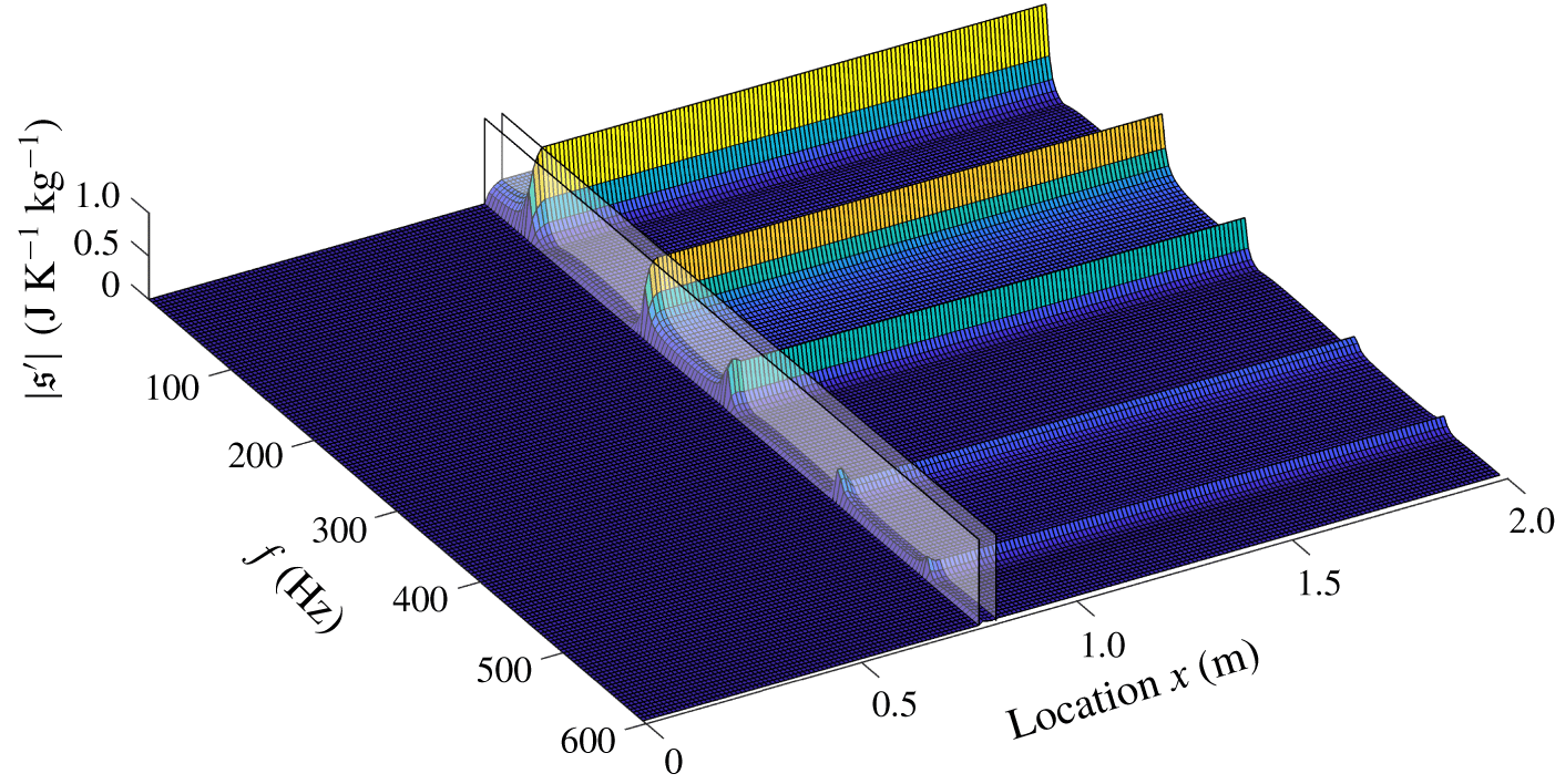
Figure 9 shows the magnitude of entropy fluctuations  $|\mathfrak{s}^{\prime }(x,\text{j}2\unicode[STIX]{x03C0}f)|$. We can see that the entropy wave has peaks at the same acoustic resonance frequencies as in (3.2) but its peaks are significantly attenuated at higher frequencies, supporting the low-pass filtering property. The entropic cutoff frequency (2.40) of this example is
 $f_{c}=238.4~\text{Hz}$.
The pressure and velocity mode shapes are shown in figures 10 and 11, respectively, and the entropy magnitude along the flow direction for each resonance frequency, call it an entropy mode shape, is shown in figure 12. The shaded box with dotted edges in each figure indicates the flame zone and the dashed horizontal lines in figure 12 indicates our theoretical estimations of entropy wave strength in (2.33).
It is first noted that our analytic prediction of entropy magnitude nicely matches with the simulation results in figure 12. Secondly, we can see that the rapid variations of entropy strength inside the flame zone in figure 12 sharply contrasts with the gentle variations of both the pressure and velocity fluctuations in figures 10 and 11, which numerically justifies our approximation (2.22).
We have found that five different flame thicknesses from  $\unicode[STIX]{x1D6E5}=0.04$ to
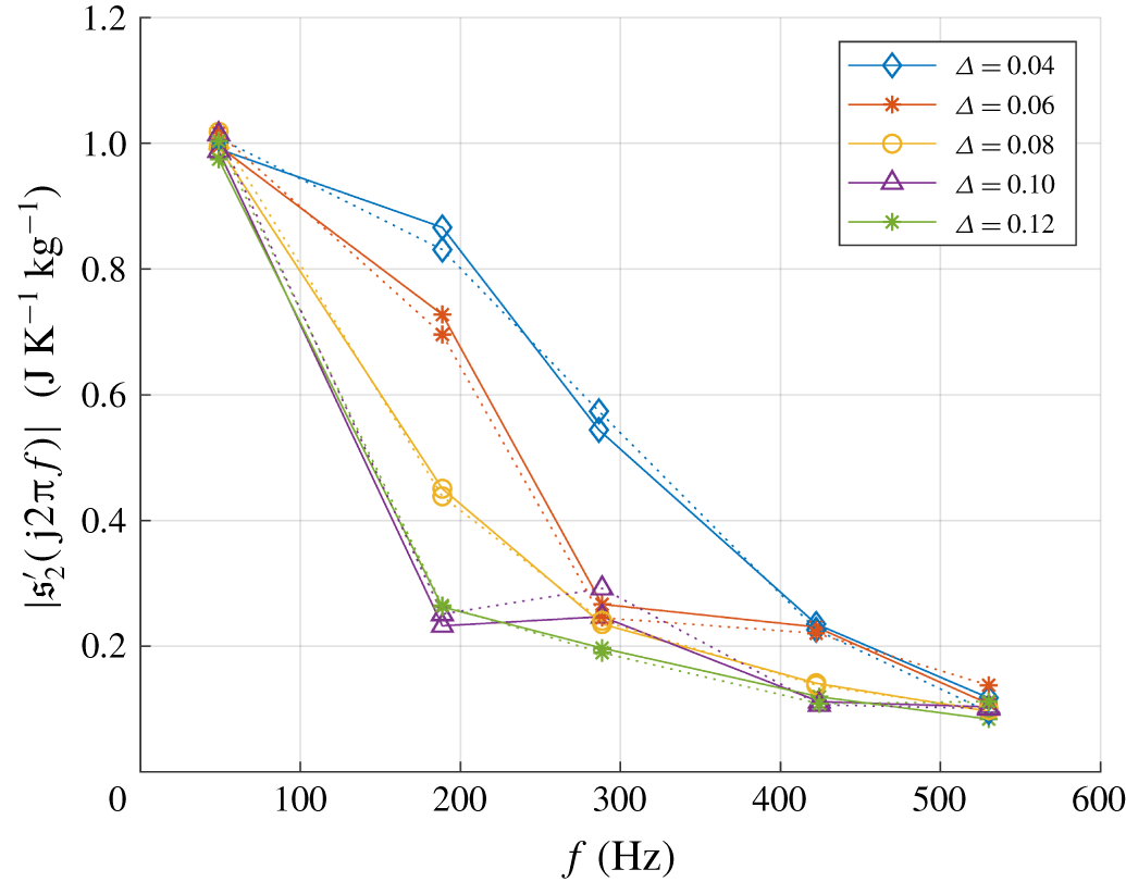
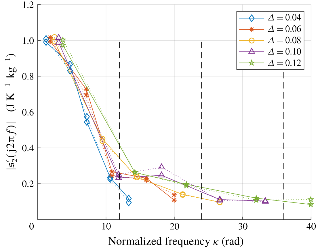
 $\unicode[STIX]{x1D6E5}=0.12~\text{m}$ give almost identical resonance frequencies. For this set of flame thicknesses, figure 13 compares the magnitude of the entropy wave at resonance frequencies, where data on the solid lines come from simulations and those on the dotted lines are theoretical predictions. The temporal low-pass filtering property of the entropy wave is again apparent in each case, and we can also see a tendency that, as flame thickness increases, the entropy magnitude at each resonance frequency steadily decreases overall. The sudden rise at the third resonance frequency 288 Hz when
 $\unicode[STIX]{x1D6E5}=0.10$ needs an explanation, and for it we plot the data of figure 13 with the normalized frequency in figure 14 in which the dashed vertical lines denote the multiples of the entropic cutoff frequency. The apparent similarity between figure 14 and a typical shape of the entropy transfer function (recall figures 3 and 4) is remarkable. This similarity suggests that the rise near 288 Hz in figure 13, which is
 $\unicode[STIX]{x1D705}=18.1$ in figure 14, corresponds to the second local peak of a typical magnitude plot of an entropy transfer function.
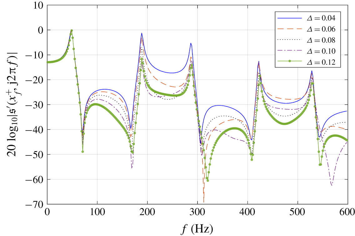
The spectrum of the entropy wave at the flame exit  $|\mathfrak{s}^{\prime }(x_{f}^{+},\text{j}2\unicode[STIX]{x03C0}f)|$ over the frequency range
 $f\in [1,600]~\text{Hz}$ is shown in figure 15 for different flame thicknesses (magnitude only). We can see that generally entropy waves of a thinner flame have more abundant frequency components, especially between resonance frequencies. The low-frequency components below 70 Hz, however, are virtually independent of the flame thickness, as expected.
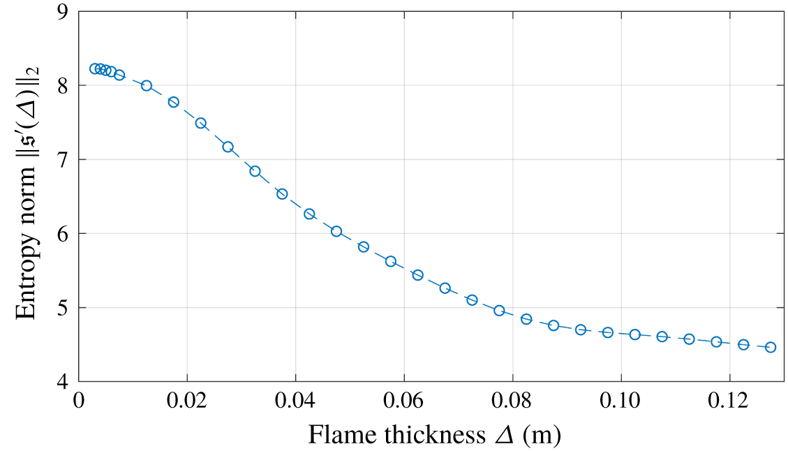
For a concrete quantification of the entropy wave strength, we considered the  $L_{2}$ norm of entropy wave defined as
 $$\begin{eqnarray}\Vert \mathfrak{s}^{\prime }(\unicode[STIX]{x1D6E5})\Vert _{2}:=\left(\int _{-\infty }^{\infty }|\mathfrak{s}^{\prime }(x_{f}^{+},t)|^{2}\,\text{d}t\right)^{1/2}=\left(\frac{1}{2\unicode[STIX]{x03C0}}\int _{-\infty }^{\infty }|\mathfrak{s}^{\prime }(x_{f}^{+},\text{j}w)|^{2}\,\text{d}w\right)^{1/2},\end{eqnarray}$$
where the second equality is Parseval’s theorem.
By approximating the integration interval in (3.3) with  $[-1200\unicode[STIX]{x03C0},1200\unicode[STIX]{x03C0}]~\text{rad}~\text{s}^{-1}$, justified from the low-pass filtering property, we obtained figure 16, which shows an indisputable inverse proportionality between flame thickness and the
 $L_{2}$ norm of the entropy wave.
4 Conclusion
By analytically solving the entropy wave equation for a one-dimensional duct with heat communications, the entropy wave generated inside the flame zone could be characterized. The analytic solution allowed us to see the entropy wave as an output of the entropy transfer functions with unsteady heat and acoustic fluctuation inputs. By investigating the zeros of the entropy transfer function, we obtained a deeper understanding of the low-pass filtering property and found that the entropic cutoff frequency is inversely proportional to the flame transit time. This means that, in the case of either a slow mean flow or a thick flame, the dynamics of entropy generation inside a flame should not be blindly ignored in an acoustic analysis. We could also explain why a thinner flame gives rise to a stronger entropy wave downstream, irrespective of the specific form of flame distribution, from a temporal-spatial filtering interpretation of the entropy wave equation.
The entropy wave solution found in this paper can be applied to the study of entropy wave dissipation and dispersion in flame chambers, and to more sophisticated acoustic models of combustors, particularly when mean flow is slow or a flame is not thin. In addition, our findings on the strength and dynamics of entropy waves can provide a more precise prediction of combustion instability when the outlet boundary condition of a combustor involves an entropy, equivalently density or temperature, fluctuation.
Acknowledgement
The author appreciates the constructive comments and suggestions of the anonymous reviewers, which significantly enhanced the quality of this paper.