1 Introduction
Two-phase bubbly flows are found in many engineering applications. They involve a wide range of scales, from the Kolmogorov scale to the macroscopic flow structures and, in between, the bubble diameter. For industrial applications such as nuclear reactor safety analysis, it is essential to correctly model the main characteristics of such flows. The wide range of flow regimes as well as the diversity of turbulence regimes require detailed information mostly related to local phenomena such as wake development, interfacial forces, bubble break-up and coalescence. Several experiments have provided useful information allowing the development of models for the interfacial forces (e.g. through the work of Tomiyama et al. (Reference Tomiyama, Tamai, Zun and Hosokawa2002)) or the turbulence (Riboux & Legendre Reference Riboux and Legendre2013; Amoura, Besnaci & Risso Reference Amoura, Besnaci and Risso2017). However, restrictions imposed by limitations of experimental methods prevent the access to bubbly flow characteristics. Thus, the only tool currently available to provide further information is direct numerical simulation (DNS) as a ‘numerical experiment’. Although several DNS studies have already been performed, none of them has yet provided the maximum amount of information that is potentially extractable from such local calculations. Following the work by Kim, Moin & Moser (Reference Kim, Moin and Moser1987) and Vreman & Kuerten (Reference Vreman and Kuerten2014) on single-phase flows, a database of statistical results for bubbly channel up-flow obtained using the computational fluid dynamics code TrioCFD is proposed here. The statistical data are available for further analysis (see http://triocfd.cea.fr/recherche/modelisation-physique/). Although several two-phase DNS calculations have already been performed (Lu & Tryggvason Reference Lu and Tryggvason2008; Santarelli & Fröhlich Reference Santarelli and Fröhlich2016; Bois et al. Reference Bois, du Cluzeau, Toutant and Martinez2017; Feng et al. Reference Feng, Yang, Mao, Lu and Tryggvason2018), there is still no database available like those of Kim et al. (Reference Kim, Moin and Moser1987) or Vreman & Kuerten (Reference Vreman and Kuerten2014) for single-phase flows. The aim of this article is to deepen our physical understanding of interfacial forces and velocity fluctuations in channel flow.
As suggested by Ilic (Reference Ilic2006), Hosokawa, Suzuki & Tomiyama (Reference Hosokawa, Suzuki and Tomiyama2012), Santarelli, Roussel & Fröhlich (Reference Santarelli, Roussel and Fröhlich2016), budgets of averaged equations can be used in order to understand the physics of two-phase flows and to bring to light first-order phenomena. Whether we are considering the one-fluid or the two-fluid formulation, the budget of the momentum equation provides information on the relative importance of interfacial forces, buoyancy, turbulence, surface tension and viscosity. Then, the phenomenology of such flows is clearer and can be analysed. Interfacial forces such as drag, lift and turbulent dispersion forces have been extensively studied in the literature but mostly on isolated bubbles in a liquid at rest or in simple linear shear flow (Tomiyama et al. Reference Tomiyama, Tamai, Zun and Hosokawa2002). However, there is still a lack of knowledge about the effect of surface tension which is classically reduced to its impact on the bubble shape. Indeed, in a point-size particle approach, the averaged surface tension source term is zero whereas in the case of resolved finite-size particles, other effects may exist. For second-order quantities, the kinetic energy budget originally proposed by Kataoka & Serizawa (Reference Kataoka and Serizawa1989) has been generalized into a tensorial transport equation (Morel Reference Morel2015). In addition to the classical terms of production, dissipation, redistribution and diffusion, this equation also contains interfacial transfer related to the kinetic energy exchanged at bubble interfaces. Many studies have already addressed these terms, numerically or experimentally, in order to propose an improved modelling of turbulence based on the kinetic energy equation. Even with optical methods, the measurement of several terms of these equations involving interfacial pressure or interfacial velocity is complicated at least, if not impossible with the state-of-the-art measuring techniques (Fujiwara, Minato & Hishida Reference Fujiwara, Minato and Hishida2004; Shawkat & Ching Reference Shawkat and Ching2011). These limitations complicate the analysis of the results whose experimental uncertainty is also difficult to estimate. On the other hand, the careful treatment with numerical tools of the interfacial quantities can lead to smaller errors (Santarelli et al. Reference Santarelli, Roussel and Fröhlich2016); the assessment of the kinetic energy budget is then simpler. Previous studies have already succeeded in measuring the terms of the kinetic energy equation, leading to an improvement of turbulence model (Ilic Reference Ilic2006; Hosokawa et al. Reference Hosokawa, Suzuki and Tomiyama2012; Santarelli et al. Reference Santarelli, Roussel and Fröhlich2016).
Turbulent fluctuations in two-phase flows are divided into bubble-induced fluctuations (BIF) and single-phase turbulence (SPT). Following this idea, the Reynolds stresses can be written as:
 $$\begin{eqnarray}\unicode[STIX]{x1D619}_{ij}=\unicode[STIX]{x1D619}_{ij}^{SPT}+\unicode[STIX]{x1D619}_{ij}^{BIF}.\end{eqnarray}$$
SPT arises from the local shear not produced directly by the wakes. It is frequently seen as ‘turbulence in the absence of bubbles’ whereas BIF represents the contribution added by the bubbles (Lance & Bataille Reference Lance and Bataille1991). Nowadays, this vision is questionable because it neglects the interaction between SPT and BIF which has been observed for instance through the phenomenon of turbulence reduction (Mazzitelli, Lohse & Toschi Reference Mazzitelli, Lohse and Toschi2003; Colin, Fabre & Kamp Reference Colin, Fabre and Kamp2012; Cisse et al. Reference Cisse, Saw, Gibert, Bodenschatz and Bec2015; Alméras et al. Reference Alméras, Mathai, Lohse and Sun2017). In most cases, the total kinetic energy is increased by BIF in regard to the single-phase equivalent. If so, the added part of turbulence is always considered as BIF without considering the possibility of SPT reduction. In order to perform the analysis of this possible interaction, SPT and BIF have to be separated. In the present study, different cases are specifically designed for such a decomposition.
Schematic decomposition of the fluctuations in two-phase bubbly flows in different parts.

Concerning the BIF, Risso et al. (Reference Risso, Roig, Amoura, Riboux and Billet2008) have proposed a splitting of the BIF into a turbulent and a non-turbulent part. The non-turbulent part (coined wake-induced fluctuations, WIF), is related to coherent structures around the bubbles such as the averaged wake or the potential flow. These fluctuations do not possess the chaotic features of turbulence leading to a dissipation process and to an energy cascade. The turbulent part (coined wake-induced turbulence, WIT), is related to wake instabilities (such as von Kármán alleys) and wake interactions. The BIF part of the Reynolds stresses is split into two contributions:
 $$\begin{eqnarray}\unicode[STIX]{x1D619}_{ij}^{BIF}=\unicode[STIX]{x1D619}_{ij}^{WIT}+\unicode[STIX]{x1D619}_{ij}^{WIF}.\end{eqnarray}$$
Moreover, different studies have shown that WIF and WIT are statistically independent, meaning that there is no interaction between them (Riboux, Risso & Legendre Reference Riboux, Risso and Legendre2010; Riboux & Legendre Reference Riboux and Legendre2013; Risso Reference Risso2016; Amoura et al. Reference Amoura, Besnaci and Risso2017; Risso Reference Risso2018). A schematic view of those different parts of turbulence is sketched in figure 1. These works brought clarity to two-phase turbulence phenomenology, but additional studies are mandatory for an improvement of turbulence modelling. The classical way to model two-phase turbulence involves only the splitting of turbulence into SPT and BIF. In order to adapt single-phase turbulence models to two-phase flows, many authors have implicitly assumed that WIF and WIT may be modelled together (Hosokawa & Tomiyama Reference Hosokawa and Tomiyama2013; Colombo & Fairweather Reference Colombo and Fairweather2015; Vaidheeswaran & Hibiki Reference Vaidheeswaran and Hibiki2017). Although there have been several attempts to use other decompositions based on physical considerations (Risso Reference Risso2018), to the best of our knowledge all turbulence models are still based on a coarse vision of two-phase flow (except for the work of Chahed, Roig & Masbernat (Reference Chahed, Roig and Masbernat2003) who proposed distinguishing between the dissipative and the non-dissipative parts of BIF). The separate study of WIT and WIF is complicated because it often relies on calculations in the reference frame of the bubbles (see Riboux & Legendre (Reference Riboux and Legendre2013) or Amoura et al. (Reference Amoura, Besnaci and Risso2017) for more details). Alternatives works such as Bouche, Roig & Risso (Reference Bouche, Roig and Risso2012) and Bouche, Roig & Risso (Reference Bouche, Roig and Risso2014) succeeded in studying WIF alone in a Hele-Shaw cell by preventing the appearance of WIT with the strong containment. Amoura et al. (Reference Amoura, Besnaci and Risso2017) also observed that the nonlinear interactions leading to WIT production do not occur for a bubble Reynolds number less than 200. Thus, for the small bubble Reynolds numbers encountered for instance in low gravity conditions, BIF is expected to be comprised of WIF exclusively, which allows the study of WIF through the analysis of the Reynolds stress transport equations. The article is organized as follows. Our simulations are described in § 2. In order to validate the front-tracking algorithm of TrioCFD briefly described in § 2, a comparison of averaged statistical quantities with the results of Lu & Tryggvason (Reference Lu and Tryggvason2008) is performed along with a mesh convergence study. Section 3 focuses on physical interpretations of the momentum budget in order to study the impact of the surface tension source term. Sections 4 and 5 deal with two-phase turbulence phenomenology and modelling. In § 4, an in-depth analysis of BIT and SPT interactions is performed. Section 5 presents an analysis of the second-order statistics of two-phase turbulence, a discussion on numerical issues for a better estimation of the Reynolds stress budget and modelling of WIF.
Numerical and physical parameters for calculations at
 $Re_{\unicode[STIX]{x1D70F}}=127$
for
 $h=1$
(the characteristic length scale of the channel). The bubble diameter is
 $d_{b}$
,
 $N_{b}$
is the number of bubbles,
 $L_{x}$
and
 $N_{x}$
are respectively the length and the number of cells in
 $x$
direction and
 $\unicode[STIX]{x0394}x^{+}=(L_{x}/N_{x})Re_{\unicode[STIX]{x1D70F}}/h$
. The Eötvös number is
 $Eo=\unicode[STIX]{x1D70C}_{l}gd_{b}^{2}/\unicode[STIX]{x1D70E}$
. The parietal Reynolds number is defined as
 $Re_{\unicode[STIX]{x1D70F}}=hu_{\unicode[STIX]{x1D70F}}/\unicode[STIX]{x1D708}_{l}$
, with
 $u_{\unicode[STIX]{x1D70F}}=\sqrt{(\unicode[STIX]{x1D707}_{l}/\unicode[STIX]{x1D70C}_{l})(\unicode[STIX]{x2202}\overline{u}/\unicode[STIX]{x2202}y|_{y=0})}$
.
 $Re_{c}=D_{h}\langle u\rangle /\unicode[STIX]{x1D708}_{l}$
is the channel Reynolds number, with the hydraulic diameter
 $D_{h}=4h$
.
 $Re_{b}=d_{b}\langle u_{r}\rangle /\unicode[STIX]{x1D708}_{l}$
is the bubble Reynolds number, with
 $u_{r}=\overline{u_{v}}^{v}-\overline{u_{l}}^{l}$
, the mean upstream relative velocity of the bubbles.
 $\unicode[STIX]{x0394}t_{ave}$
,
 $\unicode[STIX]{x0394}t_{ave}^{\unicode[STIX]{x1D70F}}$
,
 $\unicode[STIX]{x0394}t_{ave}^{\unicode[STIX]{x1D708}}$
are the time intervals within which statistical results have been measured. They are expressed respectively in time units
 $t.u.=h/\langle u\rangle$
,
 $t.u.\unicode[STIX]{x1D70F}=h/u_{\unicode[STIX]{x1D70F}}$
,
 $t.u.\unicode[STIX]{x1D708}=h^{2}/\unicode[STIX]{x1D708}$
.

2 Direct numerical simulations
The physical interpretation presented in this article is based on the ‘numerical experiments’ described in this section. Section 2.1 introduces the algorithm of TrioCFD and the numerical set-up of the different cases. Then, § 2.2 presents a code verification (benchmark) by comparing the results given by TrioCFD with the work of Lu & Tryggvason (Reference Lu and Tryggvason2008). A mesh convergence study is also performed on isolated bubbles. Finally, a general description of the results in § 2.3 gives the main mechanisms of turbulent two-phase channel flows.
2.1 Definition of simulations
The computational domain is a
 $h\unicode[STIX]{x03C0}\times 2h\times h\unicode[STIX]{x03C0}/2$
channel at
 $Re_{\unicode[STIX]{x1D70F}}=127$
(see table 1) between two vertical walls perpendicular to the direction 2 (
 $y$
). The distance between the walls is
 $2h=2$
where
 $h$
is the characteristic length of the channel. There are periodic conditions in direction 1 (
 $x$
, streamwise) and direction 3 (
 $z$
, spanwise). The flow is driven upward by a mean pressure gradient calculated to satisfy an imposed velocity gradient at the wall, while the acceleration due to gravity acts downwards (along the
 $x$
-axis). Different populations of bubbles travel in this domain (as listed in table 1). For the smallest bubbles, the cell size of the mesh is decreased to maintain a bubble resolution at approximately
 $30$
cells per bubble diameter in the wall-normal direction.
TrioCFD resolves the one-fluid equations of Kataoka (Reference Kataoka1986) as written for channel up-flow by Lu & Tryggvason (Reference Lu and Tryggvason2008):
 $$\begin{eqnarray}\unicode[STIX]{x1D735}\boldsymbol{\cdot }\boldsymbol{u}=0,\end{eqnarray}$$
 $$\begin{eqnarray}\displaystyle \frac{\unicode[STIX]{x2202}\unicode[STIX]{x1D70C}\boldsymbol{u}}{\unicode[STIX]{x2202}t}+\unicode[STIX]{x1D735}\boldsymbol{\cdot }(\unicode[STIX]{x1D70C}\boldsymbol{u}\otimes \boldsymbol{u}) & = & \displaystyle -\unicode[STIX]{x1D735}P^{\prime }+(\unicode[STIX]{x1D70C}-\langle \unicode[STIX]{x1D70C}\rangle )\boldsymbol{g}-\unicode[STIX]{x1D6FD}\boldsymbol{e}_{x}\nonumber\\ \displaystyle & & \displaystyle +\,\unicode[STIX]{x1D735}\boldsymbol{\cdot }[\unicode[STIX]{x1D707}(\unicode[STIX]{x1D735}\boldsymbol{u}+\unicode[STIX]{x1D735}^{\text{T}}\boldsymbol{u})]+\unicode[STIX]{x1D70E}\unicode[STIX]{x1D705}\boldsymbol{n}_{v}\unicode[STIX]{x1D6FF}^{i},\end{eqnarray}$$
where each of the one-fluid variables is defined as a mixture of phase variables:
 $\unicode[STIX]{x1D719}=\sum _{k}\unicode[STIX]{x1D712}_{k}\unicode[STIX]{x1D719}_{k}$
where
 $\unicode[STIX]{x1D719}_{k}$
can be
 $u_{k}$
,
 $\unicode[STIX]{x1D70C}_{k}$
,
 $\unicode[STIX]{x1D707}_{k}$
or
 $P_{k}$
, respectively the velocity, the density, the viscosity and the pressure in phase
 $k$
. Here
 $\unicode[STIX]{x1D712}_{k}$
is the phase indicator function, which is equal to 1 in phase
 $k$
and 0 otherwise. The transport equation is then
 $\unicode[STIX]{x2202}\unicode[STIX]{x1D712}_{v}/\unicode[STIX]{x2202}t+\boldsymbol{u}_{i}\boldsymbol{\cdot }\unicode[STIX]{x1D735}\unicode[STIX]{x1D712}_{v}=0$
, where
 $\boldsymbol{u}_{i}$
is the interfacial velocity of the front. Here, in the absence of phase change, the velocity is continuous across the interface and
 $\boldsymbol{u}_{i}=\boldsymbol{u}$
. Following the proposal of Lu & Tryggvason (Reference Lu and Tryggvason2008), the pressure gradient
 $\unicode[STIX]{x1D735}P$
is split into mean
 $\unicode[STIX]{x1D735}\langle P\rangle$
and fluctuating
 $\unicode[STIX]{x1D735}P^{\prime }$
parts (
 $\langle \unicode[STIX]{x1D719}\rangle$
is the space average of
 $\unicode[STIX]{x1D719}$
over the whole domain);
 $\unicode[STIX]{x1D6FD}$
is a constant source term containing the spatially averaged weight of the mixture and the driving pressure gradient so that
 $\unicode[STIX]{x1D6FD}=\unicode[STIX]{x1D735}\langle P\rangle -\langle \unicode[STIX]{x1D70C}\rangle \boldsymbol{g}$
. It corresponds to an imposed shear stress at the wall. The surface tension is
 $\unicode[STIX]{x1D70E}$
,
 $\unicode[STIX]{x1D705}=-\unicode[STIX]{x1D735}\boldsymbol{\cdot }\boldsymbol{n}_{v}$
is the local curvature and
 $\boldsymbol{n}_{v}$
is the interface normal defined by
 $\unicode[STIX]{x1D735}\unicode[STIX]{x1D712}_{v}=-\boldsymbol{n}_{v}\unicode[STIX]{x1D6FF}^{i}$
, where
 $\unicode[STIX]{x1D6FF}^{i}$
is the Dirac impulse at the interface
 $i$
.
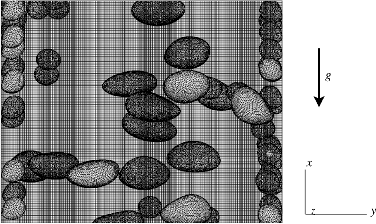
Following the proposal of Tryggvason et al. (Reference Tryggvason, Bunner, Esmaeeli and Al-Rawahi2003), a front-tracking method is used to solve this set of equations in the whole computational domain, including both the gas and liquid phases. The interface is followed by connected marker points (see figure 2). The Lagrangian markers are advected by the velocity field interpolated from the Eulerian grid. In order to preserve the mesh quality and to limit the need for a smoothing algorithm, only the normal component of the velocity field is used in the marker transport. After transport, the front is used to update the phase indicator function, the density and the viscosity at each Eulerian grid point. The Navier–Stokes equations are then solved by a projection method (Puckett et al. Reference Puckett, Almgren, Bell, Marcus and Rider1997) using fourth-order central differentiation for evaluation of the convective and diffusive terms on a fixed, staggered Cartesian grid. Fractional time stepping leads to a third-order Runge–Kutta scheme (Williamson Reference Williamson1980). In the two-step prediction–correction algorithm, a surface tension source is added to the main flow source term and to the evaluation of the convection and diffusion operators in order to obtain the predicted velocity (see Mathieu (Reference Mathieu2003) for further information). Then, an elliptic pressure equation is solved by an algebraic multigrid method to impose a divergence-free velocity field. TrioCFD has already been used for two-phase (Toutant et al. Reference Toutant, Labourasse, Lebaigue and Simonin2008, Reference Toutant, Chandesris, Jamet and Lebaigue2009a ,Reference Toutant, Chandesris, Jamet and Lebaigue b ; Toutant, Mathieu & Lebaigue Reference Toutant, Mathieu and Lebaigue2012; Bois, Fauchet & Toutant Reference Bois, Fauchet and Toutant2016; Bois Reference Bois2017; Bois et al. Reference Bois, du Cluzeau, Toutant and Martinez2017) and single-phase (Chandesris & Jamet Reference Chandesris and Jamet2006; Dupuy, Toutant & Bataille Reference Dupuy, Toutant and Bataille2018) flow studies.
Illustration of part of the computational domain with Eulerian and Lagrangian meshes for case B.

The flow is governed by dimensionless numbers (see table 1) such as the Eötvös number
 $Eo=\unicode[STIX]{x1D70C}_{l}gd_{b}^{2}/\unicode[STIX]{x1D70E}$
and the parietal Reynolds number
 $Re_{\unicode[STIX]{x1D70F}}=hu_{\unicode[STIX]{x1D70F}}/\unicode[STIX]{x1D708}_{l}$
. Five cases are studied; Sb and Ss refer to spherical cases with big and small bubbles respectively; D denotes the deformable case and B corresponds to the bidisperse case. Finally, SP is the single-phase case. The Eötvös number takes different values in the simulations with quasi-spherical bubbles (
 $Eo=0.45$
for case Sb,
 $Eo=1.36$
for case Ss) or with strongly deformable bubbles (case D,
 $Eo=4.5$
). The bidisperse case (case B) combines bubbles from cases D and Ss. Cases D and Sb are identical to those of Lu & Tryggvason (Reference Lu and Tryggvason2008) in order to perform the following code verification. Cases Ss and B have been especially designed to study separately SPT and BIF. Continuity of the viscosity at the interface and incompressibility of the flow allow us to neglect the transposed velocity gradient in the viscous operator. The density ratio of
 $10$
with a dynamic viscosity ratio of
 $1$
is in agreement with a kinematic viscosity ratio of
 $1/10$
between liquid and gas, as encountered in air/water flows. The viscosity ratio is taken as unity for convenience. The low void fraction of 3 % for monodisperse cases (6 % for case B) justifies us not considering bubble coalescence and the Eötvös numbers have been chosen such that break-up is not encountered (Lu & Tryggvason Reference Lu and Tryggvason2008).
2.2 Validation
The validation is carried out by comparing statistical profiles from the DNS to single-phase (Vreman & Kuerten Reference Vreman and Kuerten2014) and two-phase (Lu & Tryggvason Reference Lu and Tryggvason2008) flow references in the literature. In order to study statistical profiles, the ensemble averaging is defined as a temporal averaging, particularized to a space and time average by application of the ergodicity hypothesis to the periodic directions of the flow:
 $$\begin{eqnarray}\overline{\unicode[STIX]{x1D719}(y)}=\frac{1}{\unicode[STIX]{x0394}t_{ave}L_{x}L_{z}}\int _{t-\unicode[STIX]{x0394}t_{ave}/2}^{t+\unicode[STIX]{x0394}t_{ave}/2}\int _{0}^{L_{x}}\int _{0}^{L_{z}}\unicode[STIX]{x1D719}(x,y,z,\unicode[STIX]{x1D70F})\,\text{d}x\,\text{d}z\,\text{d}\unicode[STIX]{x1D70F},\end{eqnarray}$$
where
 $L_{x}$
and
 $L_{z}$
are respectively the length and depth of the channel and
 $\unicode[STIX]{x0394}t_{ave}$
is the time interval of the average expressed in time units
 $t.u.=h/\langle u\rangle$
. For a single-phase case at
 $Re_{\unicode[STIX]{x1D70F}}=180$
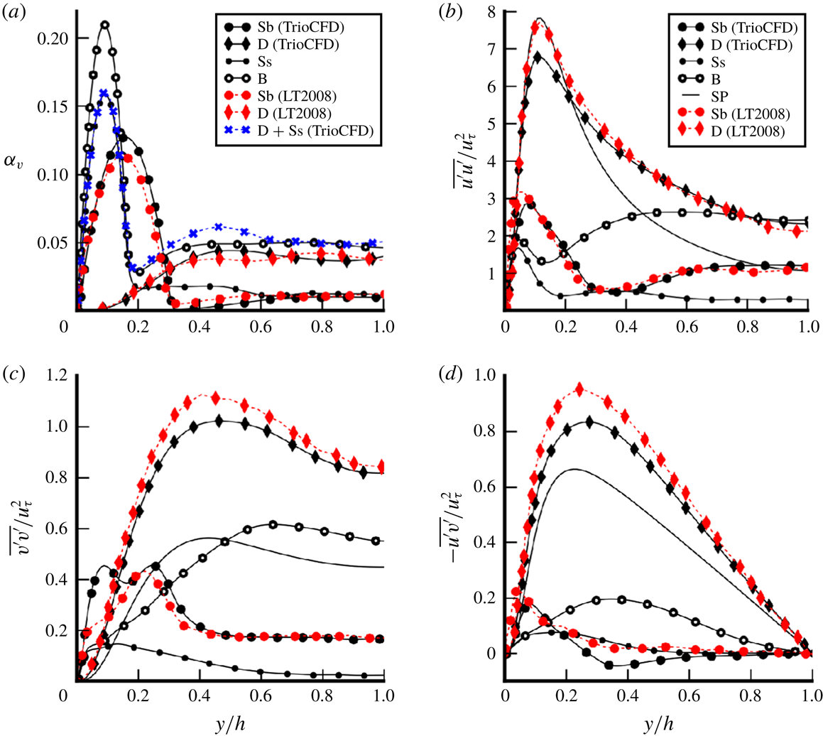
, the results of TrioCFD are very close to those of Vreman & Kuerten (Reference Vreman and Kuerten2014). Reynolds stress tensor components are presented to illustrate this validation in figure 3. For two-phase validation, the void fraction and the Reynolds stress tensor components are compared with the reference from Lu & Tryggvason (Reference Lu and Tryggvason2008) in figure 4. The results are in good agreement and the differences can probably be explained mainly by the time interval used for averages. Lu & Tryggvason (Reference Lu and Tryggvason2008) have averaged over a time interval of
 $\unicode[STIX]{x0394}t_{ave}=150$
t.u. for the spherical case and
 $\unicode[STIX]{x0394}t_{ave}=120$
t.u. for the deformable one. The results presented here have been averaged over a time interval of 140 t.u. for the spherical case and 300 t.u. for the deformable case. Indeed, our statistics are sufficiently converged to present higher-order statistics such as those of the transport equation of the Reynolds stress tensor (see § 5). However, this explanation does not clarify the presence of the second peak in figure 4(c). As in Lu & Tryggvason (Reference Lu and Tryggvason2008), in the deformable case, some break-up has been artificially removed. In the averaging time interval, only one break-up occurs for the deformable case and none for the spherical cases. The bidisperse case does not exhibit any break-up because of the slight decrease in turbulence. Thus, it can be concluded that the small amount of break-up does not disturb the statistics.
Single-phase validation: comparison between TrioCFD results and the Vreman database (Vreman & Kuerten Reference Vreman and Kuerten2014) for single-phase channel flow at
 $Re_{\unicode[STIX]{x1D70F}}=180$
.

Two-phase validation: comparison of standard quantities versus wall-normal coordinate between TrioCFD and the reference results of Lu & Tryggvason (Reference Lu and Tryggvason2008) as well as the results from our calculations (SP, Ss, Sb, D and B) at
 $Re_{\unicode[STIX]{x1D70F}}=127$
: (a) void fraction; (b)
 $\overline{u^{\prime }u^{\prime }}/u_{\unicode[STIX]{x1D70F}}^{2}$
; (c)
 $\overline{v^{\prime }v^{\prime }}/u_{\unicode[STIX]{x1D70F}}^{2}$
; (d)
 $-\overline{u^{\prime }v^{\prime }}/u_{\unicode[STIX]{x1D70F}}^{2}$
.

Mesh convergence tests on isolated bubble for
 $Re_{b}$
from
 $20$
to
 $128$
compared to experimental data of Bertakis et al. (Reference Bertakis, Großss, Grande, Fortmeier, Reusken and Pfennig2010);
 $\infty$
is the exponential extrapolation as proposed by Richardson (Reference Richardson1911) for an infinitely refined mesh.

Instantaneous illustrations of the flows. Interfaces are coloured to indicate the local curvature and the blue scale represents isovalues of the
 $\unicode[STIX]{x1D706}_{2}$
criterion (Jeong & Hussain Reference Jeong and Hussain1995).

Initially, the mesh resolution has been chosen in order to be compatible with the assessment of the Kolmogorov length scale. For the SPT, the
 $y^{+}$
criterion is used. For the BIF, an assessment of the Kolmogorov length scale is given by Risso (Reference Risso2018):
 $\unicode[STIX]{x1D702}=(\unicode[STIX]{x1D708}^{3}/\unicode[STIX]{x1D716})^{1/4}$
where
 $\unicode[STIX]{x1D716}$
is approximated by the work of buoyancy forces estimated by
 $\unicode[STIX]{x1D716}=\unicode[STIX]{x1D6FC}_{v}g\langle u_{r}\rangle$
. Considering the relative homogeneity of bubble repartition in the domain, a uniform mesh is preferred (figure 2). Confidence in this resolution has also been strengthened by additional mesh convergence study on an isolated bubble in a periodic box of
 $20d_{b}\times 5d_{b}\times 5d_{b}$
. Because the wake undergoes transition to turbulence, the resolution of the domain has to increase with the bubble Reynolds number (
 $Re_{b}=d_{b}\langle u_{r}\rangle /\unicode[STIX]{x1D708}_{l}$
where
 $\langle u_{r}\rangle$
is the relative velocity between bubbles and liquid). Cases in table 1 correspond to low gravity conditions so that the bubble Reynolds number is approximately
 $140$
for cases D and B, and even smaller for case Ss. The mesh convergence study has been performed comparing DNS of isolated bubbles with the experimental results obtained by Bertakis et al. (Reference Bertakis, Großss, Grande, Fortmeier, Reusken and Pfennig2010) at different bubble Reynolds numbers. The results are presented in table 2. A strong convergence criterion based on the accurate prediction of the terminal velocity is chosen. Indeed, the terminal velocity is more difficult to capture than the Reynolds stresses or other second-order quantities. Table 2 shows that for bubble Reynolds numbers from
 $20$
to
 $128$
, an error including numerical convergence and experimental uncertainty below
 $10\,\%$
is reached for a resolution of
 $25$
cells per diameter and it weakly depends on further mesh refinement. Further refinement is not necessary because DNS values converge towards slightly different values than experiments (
 $\infty$
is the exponential extrapolation as proposed by Richardson (Reference Richardson1911) for an infinitely refined mesh). It may be due to containment effects in our calculations or to interface contamination by surfactant in the experiment (Alves, Orvalho & Vasconcelos Reference Alves, Orvalho and Vasconcelos2005). Finally, the criterion of
 $25$
cells per diameter has been used for the DNS of table 1 (
 $28.8$
cells/diameter for cases Sb and D;
 $31.7$
cells/diameter for cases Ss and B). This mesh convergence study is performed for
 $Re_{b}<130$
. It gives confidence in the following results concerning cases Ss, D and B which are included in this range of bubble Reynolds numbers. The mesh convergence study is not extended further to case Sb (
 $Re_{b}=263$
) because this case is used solely as a validation tool for the benchmark with Lu & Tryggvason (Reference Lu and Tryggvason2008).
2.3 General remarks
Figure 5 shows the instantaneous fields for cases B, D, Ss and SP. Turbulent streaks and wakes are materialized by values near zero of the
 $\unicode[STIX]{x1D706}_{2}$
criterion (Jeong & Hussain Reference Jeong and Hussain1995). These results are in accordance with those of Lu & Tryggvason (Reference Lu and Tryggvason2008) and explain the differences in bulk Reynolds number between cases (see table 1). The strongest effect of an increasing Eötvös number is the reversal of the lift force starting from a critical value
 $Eo_{c}(Re_{\unicode[STIX]{x1D70F}}=127)\approx 2.5$
(Tryggvason et al.
Reference Tryggvason, Dabiri, Aboulhasanzadeh and Lu2013). The two cases
 $Eo=0.45$
and
 $Eo=1.36$
do not present significant differences, because they are both below
 $Eo_{c}$
. For bubbly flows, the preservation of a parietal Reynolds number
 $Re_{\unicode[STIX]{x1D70F}}=hu_{\unicode[STIX]{x1D70F}}/\unicode[STIX]{x1D708}_{l}$
corresponds to very different channel Reynolds numbers
 $Re_{c}=D_{h}\langle u\rangle /\unicode[STIX]{x1D708}_{l}$
depending on the bubble distribution (see table 1). For case D, the channel Reynolds number
 $Re_{c}\approx 7200$
is rather close to the reference single-phase flow (at
 $Re_{c}\approx 7700$
) whereas it is strongly reduced to
 $Re_{c}\approx 3000$
for case Ss. In the case of bigger spherical bubbles (case Sb), it has an intermediate value of
 $Re_{c}\approx 4000$
. Lastly, the bidisperse case (B) is strongly influenced by the smallest bubbles at the wall, but a small increase in flow rate is created by the large bubbles in the core region of the flow hence leading to a slightly higher value than case Ss,
 $Re_{c}\approx 3200$
(averaged liquid velocity profiles are also shown in figure 12
b). From figure 5, the length of the domain is satisfactory with respect to the size of turbulent structures. Indeed, bubble disturbance usually tends to a decrease of the length of the turbulent structures, so that a two-phase periodic channel can be slightly shorter than the single-phase equivalent. This is indeed the case for simulations B and Ss. However, for a typical core-peaking flow (case D), the boundary layer is free of bubbles; turbulent structures are not disturbed by bubbles and the channel length is comparable to the largest turbulent structure developing. Lu & Tryggvason (Reference Lu and Tryggvason2008) show from (2.2) that the shear stresses are balanced in a statistical steady state by the local-to-average difference in mixture weight and the mean pressure gradient
 $\unicode[STIX]{x1D6FD}$
:
 $$\begin{eqnarray}\frac{\text{d}(\unicode[STIX]{x1D70F}_{\unicode[STIX]{x1D707}}+\unicode[STIX]{x1D70F}_{turb})}{\text{d}y}-\unicode[STIX]{x1D6FD}-(\overline{\unicode[STIX]{x1D70C}(y)}-\langle \unicode[STIX]{x1D70C}\rangle )g=0,\end{eqnarray}$$
where
 $\unicode[STIX]{x1D70F}_{\unicode[STIX]{x1D707}}=\unicode[STIX]{x1D707}_{l}\unicode[STIX]{x2202}\overline{u}/\unicode[STIX]{x2202}y$
and
 $\unicode[STIX]{x1D70F}_{turb}=-\overline{\unicode[STIX]{x1D70C}u^{\prime }v^{\prime }}$
. For case Ss, the bubble distribution is in agreement with the hydrostatic model proposed in Lu, Biswas & Tryggvason (Reference Lu, Biswas and Tryggvason2006) (not shown here); the shear-induced lift force creates bubble clustering at the wall by a kind of Magnus effect until the average weight of the mixture in the core flow compensates for the pressure gradient. Then, the bubble distribution reaches hydrostatic equilibrium. When the averaged mixture weight compensates for the pressure gradient (as in cases Ss and Sb), Lu & Tryggvason (Reference Lu and Tryggvason2008) as well as Dabiri & Bhuvankar (Reference Dabiri and Bhuvankar2016) observed an overall reduction in turbulent structures because of the shear-stress balance in a statistical steady state (
 $\text{d}\unicode[STIX]{x1D70F}_{turb}/\text{d}y\approx 0$
). In that case, all the flow complexity is restricted to the thin layer between the wall and the bubbles where dissipation is the greatest. The proximity between wall and bubbles combined with the relative velocity caused by buoyancy create strong local shear at the wall easily satisfying the criterion
 $Re_{\unicode[STIX]{x1D70F}}=127$
, thus explaining the equilibrium between mixture weight and pressure gradient in the bulk.
The core-peaked profile of the void fraction for case D in figure 4(a) shows the reversal of the lift force caused by bubble deformability. Ervin & Tryggvason (Reference Ervin and Tryggvason1997) explain this phenomenon by a reversal of the total vorticity inside the bubble caused by the flattened shapes of deformable bubbles. Thus, the mean void fraction reveals a typical core-peaking distribution. In order to reach
 $Re_{\unicode[STIX]{x1D70F}}=127$
, the turbulent boundary layer then freely develops in the absence of bubbles (figure 5 shows that the classical streaks of the wall-induced turbulence in case D are similar to the streaks of case SP).
3 Surface tension effect
This section presents an analysis of two complementary formulations of the momentum balance in two-phase flows. With the first, which employs a one-fluid averaged momentum equation, study of the surface tension source term is possible because it appears directly in the equations (§ 3.1). The second formulation, which employs two-fluid averaged momentum equations, links the interfacial forces to the surface tension source term (§ 3.2).
3.1 One-fluid averaged momentum equation
Integrating the averaged equation (2.2) at statistical equilibrium gives the averaged stress equation:
 $$\begin{eqnarray}\displaystyle 0 & = & \displaystyle \underbrace{-\int _{0}^{y}\unicode[STIX]{x1D735}\overline{P^{\prime }}\,\text{d}y}_{DP}+\underbrace{\int _{0}^{y}[(\overline{\unicode[STIX]{x1D70C}}-\langle \unicode[STIX]{x1D70C}\rangle )\boldsymbol{g}-\unicode[STIX]{x1D6FD}\boldsymbol{e}_{x}]\,\text{d}y}_{S}+\underbrace{\int _{0}^{y}\unicode[STIX]{x1D735}\boldsymbol{\cdot }\overline{\unicode[STIX]{x1D749}}\,\text{d}y}_{D\unicode[STIX]{x1D70F}}\nonumber\\ \displaystyle & & \displaystyle \underbrace{-\int _{0}^{y}\unicode[STIX]{x1D735}\boldsymbol{\cdot }(\overline{\unicode[STIX]{x1D70C}\boldsymbol{u}^{\prime }\otimes \boldsymbol{u}^{\prime }})\,\text{d}y}_{D\unicode[STIX]{x1D619}_{ij}}+\underbrace{\int _{0}^{y}\overline{\unicode[STIX]{x1D70E}\unicode[STIX]{x1D705}\boldsymbol{n}_{v}\unicode[STIX]{x1D6FF}^{i}}\,\text{d}y}_{\boldsymbol{M}_{\unicode[STIX]{x1D70E}}}.\end{eqnarray}$$
Each term of (3.1) is plotted in figure 6 for the four comparable cases (namely SP, Ss, D and B). In the interest of readability, the results are presented as stresses instead of forces since they allow ranking of the different terms. Obviously, for single-phase flow (SP), the term
 $M_{\unicode[STIX]{x1D70E}}$
and the first term of
 $S$
are removed from (3.1) and one-fluid variables become classical variables. Figure 6(a) confirms the observations in § 2.3 that the typical impact of bubble wall clustering in the case Ss is a balance between the averaged weight of the mixture and the pressure gradient source term in the bulk of the channel (
 $S\approx cte$
for
 $y/h>0.2$
); thus, this flow is almost laminar (
 $D\unicode[STIX]{x1D619}_{ij}\approx 0$
). Case B presents a similar behaviour with a slight increase of turbulence in the bulk due to the presence of deformable bubbles. In contrast, the turbulent term
 $D\unicode[STIX]{x1D619}_{ij}$
is bigger for case D, slightly above the SP value, due to the core-peaking process described in § 2.3 which does not disturb the turbulent boundary layer development and adds additional fluctuations due to the presence of bubbles in the bulk.
Contributions to the one-fluid equation (3.1) versus the wall-normal coordinate: (a) streamwise momentum budget; (b) wall-normal momentum budget for cases D and SP; (c) wall-normal momentum budget for cases Ss and B. The first parts of the legends identify the terms of the momentum equation by a colour and/or a line style (dashed or solid line). The second part (in black) identifies the case by a specific marker (only the case SP is plotted without marker).

3.1.1 Surface tension and wall repulsion
At the wall, the interpretation of the forces changes. For instance, in figure 4(a), the void-fraction peak at
 $y/h\approx 0.15$
for case Sb can easily be interpreted as the expression of a repulsive force from the wall (see, e.g. Antal, Lahey & Flaherty Reference Antal, Lahey and Flaherty1991). However, this type of interpretation leads to a misunderstanding of the wall effect. Actually, the position of the void-fraction peak is determined by the finite size of the bubbles and corresponds here to the location of the centre of gravity of wall-peaking bubbles. Thus, the apparent repulsive effect is not a hydrodynamic force but a manifestation of the surface tension force coming from the averaging operator and the use of a particle approach. In order to quantify the bubble size-induced repulsive force, Lubchenko et al. (Reference Lubchenko, Magolan, Sugrue and Baglietto2017) have proposed a new closure that is relevant to further investigations based on DNS data. This sort of consideration arises for any variable linked to interfacial position. In particular, the surface tension source term
 $\boldsymbol{M}^{\unicode[STIX]{x1D748}}$
presents similar features with void fraction profiles in figure 6(c). Further investigations are required to understand the consequences of this non-Eulerian effect.
3.1.2 Surface tension and dispersion
From the interaction forces point of view, the dispersion of bubbles in the wall-normal direction is usually assumed to be proportional to the turbulent kinetic energy (Reeks Reference Reeks1991). This force is called turbulent dispersion (Lopez de Bertodano Reference Lopez de Bertodano1998; Laviéville et al.
Reference Laviéville, Mérigoux, Guingo, Baudry and Mimouni2015). Figure 4(c) shows that cases D and B have very different levels of root-mean-square (r.m.s.) velocity in the wall-normal component, which is a direct consequence of the lower flow rate for case B. Thus, most models will predict a large increase in the dispersion phenomenon in case D whereas figure 4(a) shows that the averaged void fractions are equally spread for both cases for
 $y/h>d_{b}$
, hence suggesting similar levels of dispersion. Additionally, figure 7 shows the individual wall-normal positions of large bubbles over time in cases D and B. The bubbles present very similar oscillations of the trajectory in both cases with similar frequencies and magnitudes. Considering the wide difference of surrounding turbulence from the liquid phase between cases B and D, this oscillating trajectory can be associated with an inherent feature of the collective swarm of bubbles. Here, the oscillating trajectory of bubbles makes clear the presence of bubble interactions. For instance, a bubble located in the wake of another bubble is subjected to the local shear induced by the wake. The reaction of the bubble then depends on its deformation. For
 $Eo<Eo_{c}$
, the bubble is expelled from the wake and Ervin & Tryggvason (Reference Ervin and Tryggvason1997) have shown that a horizontal alignment of bubbles is expected in this case. For the present case where
 $Eo>Eo_{c}$
, the bubbles preferentially stay in the wake and a verticalalignment is expected for a pair of bubbles in quiescent liquid. However, neither of the two configurations is observed here. Consequently, a more complicated interaction of the collective swarm leads to the dispersion of bubbles. Hence, it is necessary to analyse thoroughly the momentum equation in order to understand the interfacial forces responsible for dispersion.
Wall-normal positions of the
 $21$
large bubbles in case D (a); and in case B (b); on a time interval of 100 s.

In the streamwise direction, the momentum budget for deformable bubbles in figure 6(a) shows similar trends to those seen in single-phase channel flow where the pressure gradient source term is compensated by only viscous and turbulent shear. In the two-phase case, the modified source term (
 $S$
) is also compensated for by these two contributions. In the axial direction, the surface tension term is negligible but the transverse component (figure 6
b) brings other observations. Even if the surface tension energy is a particle-size effect, the averaged surface tension source term in the wall-normal direction is directly correlated with the averaged void fraction
 $$\begin{eqnarray}\displaystyle \boldsymbol{M}_{\unicode[STIX]{x1D70E}}\boldsymbol{\cdot }\boldsymbol{e}_{y}=\int _{0}^{y}\overline{\unicode[STIX]{x1D70E}\unicode[STIX]{x1D705}\boldsymbol{n}_{v}\unicode[STIX]{x1D6FF}^{i}}\boldsymbol{\cdot }\boldsymbol{e}_{y}=-\int _{0}^{y}\overline{\unicode[STIX]{x1D70E}\unicode[STIX]{x1D705}\unicode[STIX]{x2202}_{y}\unicode[STIX]{x1D712}_{v}} & = & \displaystyle \overline{\unicode[STIX]{x1D70E}\unicode[STIX]{x1D705}}^{i}[\unicode[STIX]{x1D6FC}_{v}(y)-\underbrace{\unicode[STIX]{x1D6FC}_{v}(0)}_{=0}]+C_{\unicode[STIX]{x1D705}}^{n},\nonumber\\ \displaystyle & {\approx} & \displaystyle \overline{\unicode[STIX]{x1D70E}\unicode[STIX]{x1D705}}^{i}\unicode[STIX]{x1D6FC}_{v}(y),\end{eqnarray}$$
where
 $\overline{\unicode[STIX]{x1D719}}^{i}=\overline{\unicode[STIX]{x1D719}\unicode[STIX]{x1D6FF}^{i}}/\overline{\unicode[STIX]{x1D6FF}^{i}}$
is the interfacial average;
 $C_{\unicode[STIX]{x1D705}}^{n}$
is the cross-correlation term between the curvature and the normal to the interface. At first order,
 $C_{\unicode[STIX]{x1D705}}^{n}$
can be neglected because
 $\boldsymbol{M}_{\unicode[STIX]{x1D70E}}\boldsymbol{\cdot }\boldsymbol{e}_{y}$
is proportional to
 $\unicode[STIX]{x1D6FC}_{v}$
(see the shapes of the void-fraction profile of case D in figure 4
a and of
 $\boldsymbol{M}_{\unicode[STIX]{x1D70E}}$
in figure 6
b). Even though the mean contribution of the surface tension source term on a bubble is zero, equation (3.2) shows that the surface tension source term of a swarm is not cancelled at the bubble scale and becomes significant in the wall-normal component of the momentum budget. Consequently, the question arises about the impact of the surface tension term (figure 6
b) on bubble migration. Indeed, in the wall-normal component, the momentum equation is related to the migration phenomenon. The statistical equilibrium of the wall-normal component is a balance between surface tension, pressure and turbulence. For the single-phase case, turbulence
 $D\unicode[STIX]{x1D619}_{ij}$
and pressure
 $DP$
are opposed in figure 6(b), but the surface tension source term
 $M^{\unicode[STIX]{x1D70E}}$
adds an imbalance for two-phase flow. For less turbulent cases Ss and B (figure 6
c), the pressure term
 $DP$
balances the surface tension
 $M^{\unicode[STIX]{x1D70E}}$
close to the wall, thus reflecting a strong increase of the pressure in the vapour phase related to the local Laplace law at the interfaces. For case D and in the bulk for case B, the balance deviates from the case SP to compensate for the surface tension term. Our results indicate that surface tension should be taken into account. This analysis is consistent with discussions on other mechanisms that may be implicated in the dispersion process.
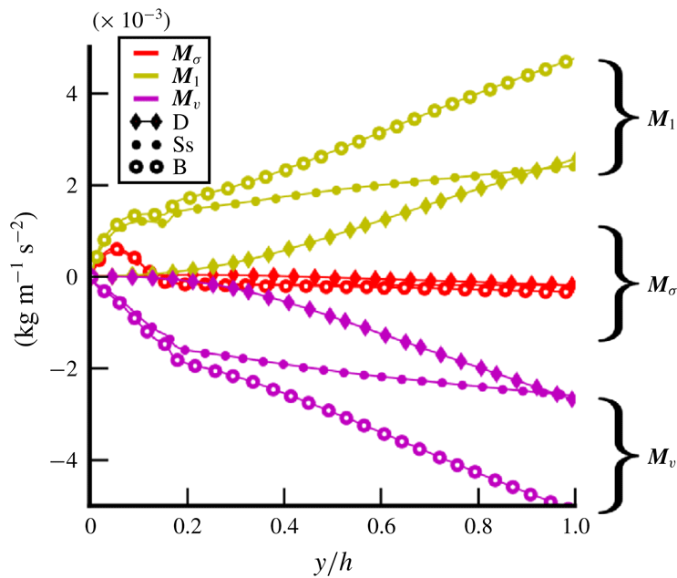
Streamwise components of the two-fluid interfacial terms in (3.4) versus the wall-normal coordinate. The first three items of the legend identify the interfacial term by a colour and/or a line style (dashed or solid line). The second part (in black) identifies the case by a specific marker.

3.2 Two-fluid averaged momentum equation
Multiplying the Navier–Stokes equation in phase
 $k\in [l,v]$
by the indicator function
 $\unicode[STIX]{x1D712}_{k}$
and averaging leads, at statistical equilibrium, to the integrated version of the phase momentum balance:
 $$\begin{eqnarray}\displaystyle -\underbrace{\int _{0}^{y}\overline{P_{i}^{\prime }\unicode[STIX]{x1D735}\unicode[STIX]{x1D712}_{k}-\unicode[STIX]{x1D70F}_{i}\boldsymbol{\cdot }\unicode[STIX]{x1D735}\unicode[STIX]{x1D712}_{k}}\,\text{d}y}_{M_{k}} & = & \displaystyle \underbrace{-\int _{0}^{y}\unicode[STIX]{x1D735}(\unicode[STIX]{x1D6FC}_{k}\overline{P_{k}^{\prime }}^{k})\,\text{d}y}_{DP_{k}}+\underbrace{\int _{0}^{y}[\unicode[STIX]{x1D6FC}_{k}(\unicode[STIX]{x1D70C}_{k}-\langle \unicode[STIX]{x1D70C}\rangle )\boldsymbol{g}-\unicode[STIX]{x1D6FC}_{k}\unicode[STIX]{x1D6FD}\boldsymbol{e}_{z}]\,\text{d}y}_{S_{k}}\nonumber\\ \displaystyle & & \displaystyle +\,\underbrace{\int _{0}^{y}\unicode[STIX]{x1D735}\boldsymbol{\cdot }\unicode[STIX]{x1D6FC}_{k}\overline{\unicode[STIX]{x1D70F}_{k}}^{k}\,\text{d}y}_{D\unicode[STIX]{x1D70F}_{k}}\underbrace{-\int _{0}^{y}\unicode[STIX]{x1D735}\boldsymbol{\cdot }(\unicode[STIX]{x1D6FC}_{k}\overline{\unicode[STIX]{x1D70C}_{k}\boldsymbol{u}_{\boldsymbol{k}}^{\prime }\otimes \boldsymbol{u}_{\boldsymbol{k}}^{\prime }}^{k})\,\text{d}y}_{D\unicode[STIX]{x1D619}_{ij}^{k}},\end{eqnarray}$$
 $$\begin{eqnarray}\boldsymbol{M}_{l}+\boldsymbol{M}_{v}=\boldsymbol{M}_{\unicode[STIX]{x1D70E}}.\end{eqnarray}$$
In this equation,
 $\overline{\unicode[STIX]{x1D719}_{k}}^{k}$
is the phase average defined as
 $\overline{\unicode[STIX]{x1D719}_{k}}^{k}=\overline{\unicode[STIX]{x1D712}_{k}\unicode[STIX]{x1D719}_{k}}/\overline{\unicode[STIX]{x1D712}_{k}}$
. This formulation reveals the term
 $\boldsymbol{M}_{k}$
corresponding to the averaged force exerted by the interface on phase
 $k$
. This formulation is linked to the one-fluid formulation by the jump conditions at the interfaces, at the origin of the relation
 $\boldsymbol{M}_{l}+\boldsymbol{M}_{v}=\boldsymbol{M}_{\unicode[STIX]{x1D70E}}$
;
 $\boldsymbol{M}_{k}$
is classically modelled by the sum of different forces such as drag, lift and turbulent dispersion forces. From DNS, it is calculated as the residue of the right-hand side of (3.3), because its direct evaluation would rely on locally discontinuous fields evaluated at the interface and this would lead to significant interpolation errors.
Figures 8 and 9 show the results obtained for interfacial forces in the axial and wall-normal directions. The consistency of our results is verified because
 $\boldsymbol{M}_{v}+\boldsymbol{M}_{l}$
fits with the surface tension source term
 $\boldsymbol{M}_{\unicode[STIX]{x1D70E}}$
according to (3.4). In the streamwise direction, interfacial forces are compensated for by buoyancy. The one-fluid surface tension source term
 $\boldsymbol{M}_{\unicode[STIX]{x1D748}}$
is negligible compared with
 $\boldsymbol{M}_{k}$
(the drag force) in figure 8. Thus, the surface tension contribution does not play a significant role in the prediction of the terminal bubble velocity in the
 $x$
direction and the action/reaction principle is applicable (
 $\boldsymbol{M}_{\boldsymbol{l}}=-\boldsymbol{M}_{\boldsymbol{v}}$
).
Wall-normal components of the two-fluid interfacial terms in (3.4) versus the wall-normal coordinate: (a) case D; (b) cases Ss and B. The first parts of the legends identify the interfacial term by a colour and/or a line style (dashed or solid line). The second part (in black) identifies the case by a specific marker.

In the wall-normal direction, interfacial forces are responsible for bubble migration. Figures 9(a) and 9(b) show these forces for cases D, Ss and B. Both
 $\boldsymbol{M}_{l}$
and
 $\boldsymbol{M}_{v}$
have positive values for case D, Ss and B. This is allowed by the role of surface tension energy. However, giving a physical interpretation for the impact of surface tension on bubble migration is difficult; its importance in the momentum budget in the direction of migration is clearly demonstrated and should exhort the research in this direction. Further complementary studies are necessary. They should involve the analysis of local instantaneous fields around the bubbles.
4 Analysis of SPT and BIF
As already mentioned in the introduction, the total fluctuations of the flow are comprised of SPT and BIF (1.1), but to the best of our knowledge, there is no methodology that allows us to identify properly SPT and BIF. In this section, a procedure to achieve this distinction is proposed; then, we begin to analyse the interaction between SPT and BIF from the comparison of the different Reynolds stress profiles. Further understanding of the mechanisms involved are presented with the analysis of the Reynolds stress equation in § 5. The methodology used for case comparisons is presented first and then applied to the Reynolds stresses. Further discussions are added at the end of this section. The same methodology is also applied in § 5 to the Reynolds stress transport equation. Based on the classical decomposition of the Reynolds stresses into SPT and BIF, we introduce the following notations for the total Reynolds stress tensor in cases B, Ss and D:
 $$\begin{eqnarray}\displaystyle & \displaystyle \unicode[STIX]{x1D619}_{ij,B}=\unicode[STIX]{x1D619}_{ij,B}^{SPT}+\unicode[STIX]{x1D619}_{ij,B}^{BIF}+\unicode[STIX]{x1D619}_{ij,B}^{bif}, & \displaystyle\end{eqnarray}$$
 $$\begin{eqnarray}\displaystyle & \displaystyle \unicode[STIX]{x1D619}_{ij,Ss}=\unicode[STIX]{x1D619}_{ij,Ss}^{SPT}+\unicode[STIX]{x1D619}_{ij,Ss}^{bif}, & \displaystyle\end{eqnarray}$$
 $$\begin{eqnarray}\displaystyle & \displaystyle \unicode[STIX]{x1D619}_{ij,D}=\unicode[STIX]{x1D619}_{ij,D}^{SPT}+\unicode[STIX]{x1D619}_{ij,D}^{BIF}, & \displaystyle\end{eqnarray}$$
where the subscripts refer to the case considered. The exponent
 $bif$
denotes the impact of small bubbles whereas
 $BIF$
refers to big bubble contributions hence the bidisperse case B has one contribution of bubble-induced fluctuations for each population of bubbles (bif+BIF).
4.1 Methodology to identify SPT and BIF
From cases B, Ss, D and SP, the study of interactions between SPT and BIF is allowed. A three step analysis pictured in figure 10 is proposed in order to quantify the impact of the deformable bubbles on the SPT. The methodology is the following:
(i) Extract from cases Ss and B the BIF induced by deformable bubbles
 $\unicode[STIX]{x1D619}_{ij,B}^{BIF}$
(figure 10
a).
(ii) Justify the assumption of equality between BIF induced by deformable bubbles in case D (
$\unicode[STIX]{x1D619}_{ij,D}^{BIF}$
) and in case B (
$\unicode[STIX]{x1D619}_{ij,B}^{BIF}$
) (transition between (a) and (b) in figure 10).(iii) Extract
$\unicode[STIX]{x1D619}_{ij,D}^{SPT}$
in case D (figure 10
b) and compare it to SPT in the reference single-phase flow (figure 10
c).


The results of this approach are presented in figure 13 and discussed in § 4.2.
Sketch of the methodology for the study of interaction between SPT and BIF from cases B, Ss, D and SP.

Probability density function of the axial velocity obtained for cases B, D and SP in the centre of the channel (
 $0.9<y/h<1.1$
). (b) Instantaneous axial velocity field of case B.

(i) Extract from cases Ss and B the BIF induced by deformable bubbles
$\unicode[STIX]{x1D619}_{ij,B}^{BIF}$
: BIF increases with bubble spreading and with increasing relative velocity. Figures 4(b), 4(c) and 4(d) show that case Ss is less turbulent than case Sb and strongly less turbulent than case SP. The decrease of the Reynolds stresses in comparison with the case SP is in agreement with the flow-rate reduction. Thus, it cannot be interpreted as a turbulence reduction phenomenon, because the cases have very different flow rates. Concerning the difference between Ss and Sb, an increased amount of wall surface is lined with bubbles in case Ss, so the transmission of turbulence between the wall and the bulk is even more complicated than for case Sb. Eventually, case Ss is almost laminar in the centre of the channel (see § 3.1), and thus case B is almost purely BIF; indeed, the bulk is then a kind of bubble swarm without any impact of the wall, because spherical bubbles act as a shield (
$\unicode[STIX]{x1D619}_{ij,Ss}^{SPT}\approx 0$
). Then, case B allows the study of BIF in the core region without the influence of SPT, which is suppressed by the layer of small bubbles at the wall. Figure 4(a) shows that the migrations of spherical and deformable bubbles are rather independent (
$\unicode[STIX]{x1D6FC}_{D}+\unicode[STIX]{x1D6FC}_{Ss}\approx \unicode[STIX]{x1D6FC}_{B}$
) justifying the separation of their independent contribution to the BIF in (4.1). Thus, spherical bubbles move toward the wall and case B (bidisperse) is similar to case Ss (small spherical bubbles) with deformable bubbles added to the bulk. This interpretation is reinforced by figure 12(b) where the liquid velocity profiles close to the wall (
$y/h<0.3$
) of cases B and Ss are almost identical. For
$y/h>0.3$
, a slight increase of the liquid velocity (compared to case Ss) is observed due to the presence of the deformable bubbles in case B. This increase is small because of the low gravity conditions (
$u_{r}<\overline{u_{l}}^{l}$
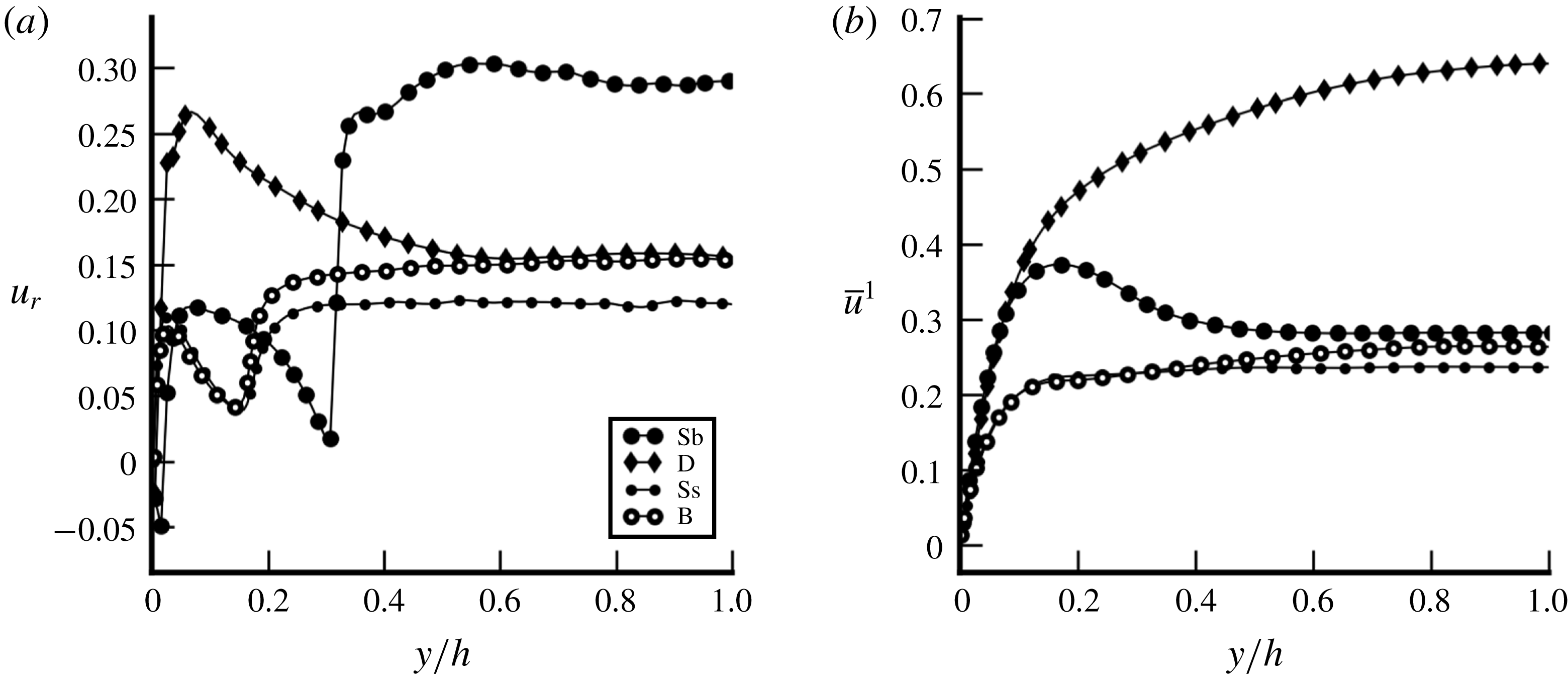
) combined with moderate void fraction. In such configurations, the mean liquid velocity is not sensitive to the evolution of the relative velocity or of the void fraction. Other cases (Ss, Sb and B) show rather similar and flat profiles in the centre of the channel. A sharp increase in the relative velocity of case Sb is observed in figure 12(a) at
$y/h=0.3$
(corresponding to the diameter of the bigger bubbles). It is due to the sudden transition between the large majority of bubbles sliding against the wall and the few others which rise faster, further away from the wall (the same non-Eulerian effect is seen for instance in figure 15). Formally, we can identify: (4.4)$$\begin{eqnarray}\displaystyle & \displaystyle \unicode[STIX]{x1D619}_{ij,Ss}^{SPT}=\unicode[STIX]{x1D619}_{ij,B}^{SPT}, & \displaystyle\end{eqnarray}$$
(4.5)Bringing together (4.1), (4.2), (4.4) and (4.5), the fluctuations induced by deformable bubbles in case B are:$$\begin{eqnarray}\displaystyle & \displaystyle \unicode[STIX]{x1D619}_{ij,Ss}^{bif}=\unicode[STIX]{x1D619}_{ij,B}^{bif}. & \displaystyle\end{eqnarray}$$
(4.6)This equation is illustrated by figure 10(a) where$$\begin{eqnarray}\unicode[STIX]{x1D619}_{ij,B}^{BIF}=\unicode[STIX]{x1D619}_{ij,B}-\unicode[STIX]{x1D619}_{ij,Ss}.\end{eqnarray}$$
$\unicode[STIX]{x1D619}_{ij,B}^{BIF}$
is shown by the purple area.(ii) Justify the assumption of equality between BIF induced by deformable bubbles in case D
$(\unicode[STIX]{x1D619}_{ij,D}^{BIF})$
and in case B (
$\unicode[STIX]{x1D619}_{ij,B}^{BIF}$
): in order to discuss this assumption, the physical nature of BIF in cases B and D has to be understood. Additional knowledge is provided by the probability density function (pdf) of the axial velocity fluctuations plotted in figure 11(a). These pdfs have been calculated on cells in the centre of the channel (
$0.9<y/h<1.1$
) for the three cases SP, B and D at a random time step of the steady state. As expected, the distribution of the velocity fluctuations in case SP follows a Gaussian distribution. In contrast, pdfs of cases B and D present an offset towards positive values. This behaviour of the pdf has been widely studied by Risso (Reference Risso2016) and corresponds to the impact of WIF due to the liquid dragged in the bubble path. The shape of the pdf in cases B and D indicates that BIF is almost entirely comprised of WIF. As said in the introduction, in the present low gravity conditions, the WIF is expected to be the biggest contribution in BIF Reynolds stresses. This interpretation is confirmed in figure 11(b) where velocity fluctuations in case B are mostly related to the wake behind each bubble. Then, the following conclusions can be drawn:(1) The repartitions of deformable bubbles are similar between cases B and D (see figure 4 a). In case B, small bubbles are mainly located at the wall and deformable bubbles mainly in the bulk. Then, the probability of interaction between the two kinds of wakes is low.
(2) For a given Eötvös number, the WIF magnitude is only related to the bubble Reynolds number and therefore to the relative velocity of bubbles. Figure 12(a) shows that cases D and B have the same relative velocity in the bulk of the channel (
$y/h>0.5$
), so that the r.m.s. velocities related to WIF are expected to be equal in that part of the flow.(3) The only difference between deformable bubbles in cases B and D is the surrounding SPT. In case B, as was already stated, the SPT is missing because of the small bubbles at the wall. At this point, the only convincing reason for WIF in case D to be different from WIF in case B would be a modulation of the WIF by the SPT but the hypothesis of a modulation of the SPT by the bubbles is far more convincing. Indeed, the fact that cases D and B have exactly the same level of turbulence in the bulk of the channel could suggest that all the SPT has disappeared for
$y/h>0.8$
. The SPT would have had an impact on the averaged wake of the bubbles and on the potential flow around them. Then the physical interpretation of the turbulence reduction could have come from a reduction of the wake length due to turbulent structures crossing them or to a stronger exponential decay of the wake. But such a phenomenon is not observed in our simulations nor in the literature whereas modulation of SPT by the presence of bubbles is a known phenomenon (Colin et al.
Reference Colin, Fabre and Kamp2012; Alméras et al.
Reference Alméras, Mathai, Lohse and Sun2017). In figure 11(a), the right tails of the pdfs, linked to the decrease of the wakes, almost perfectly overlap between cases B and D. This suggests that the exponential decay of the wake is not impacted by the surrounding SPT and is then very similar in both cases, hence leading to the same amount of WIF in both cases.
Figure 12.(a) Relative and (b) liquid velocity versus wall-normal coordinate.
Based on these statements, there is no reason for WIF in case D to be different from WIF in case B. Thus, with the (4.6), one gets an estimate for the BIF generated by deformable bubbles in cases D and B:
(4.7)$$\begin{eqnarray}\unicode[STIX]{x1D619}_{ij,D}^{BIF}=\unicode[STIX]{x1D619}_{ij,B}^{BIF}=\unicode[STIX]{x1D619}_{ij,B}-\unicode[STIX]{x1D619}_{ij,Ss}.\end{eqnarray}$$
(iii) Extract the SPT in the presence of deformable bubbles in case D and compare it to SPT without bubbles (case SP): the SPT Reynolds stresses of case D are estimated by removing the BIF contribution given by (4.7) from the total Reynolds stresses:
(4.8)This equation is illustrated in figure 10(c).$$\begin{eqnarray}\displaystyle \unicode[STIX]{x1D619}_{ij,D}^{SPT} & = & \displaystyle \unicode[STIX]{x1D619}_{ij,D}-\unicode[STIX]{x1D619}_{ij,D}^{BIF},\nonumber\\ \displaystyle & = & \displaystyle \unicode[STIX]{x1D619}_{ij,D}-(\unicode[STIX]{x1D619}_{ij,B}-\unicode[STIX]{x1D619}_{ij,Ss}).\end{eqnarray}$$
$\unicode[STIX]{x1D619}_{ij,D}^{SPT}$
is shown by the red area. Then, the comparison between
$\unicode[STIX]{x1D619}_{ij,D}^{SPT}$
and the SPT from case SP gives a quantitative assessment of the interaction between SPT and BIF (i.e. the turbulence modulation due to the presence of bubbles).


As previously mentioned in the introduction, the interaction between SPT and BIF is classically neglected (Lance & Bataille Reference Lance and Bataille1991) even if several phenomena, such as the turbulence reduction, are in contradiction with this hypothesis. In the case of turbulence increase, to the best of our knowledge, no methodology before this one has been proposed to assess the impact of a possible interaction. If SPT and BIF do not have interactions, finding
 $\unicode[STIX]{x1D619}_{ij,D}^{SPT}$
equal to the total Reynolds stresses of case SP is expected.
SPT Reynolds stresses versus wall-normal coordinate (a)
 $\overline{u^{\prime }u^{\prime }}/u_{\unicode[STIX]{x1D70F}}^{2}$
; (b)
 $\overline{v^{\prime }v^{\prime }}/u_{\unicode[STIX]{x1D70F}}^{2}$
; (c)
 $\overline{u^{\prime }v^{\prime }}/u_{\unicode[STIX]{x1D70F}}^{2}$
. D
 $-$
B
 $+$
Ss denotes the reconstructed SPT Reynolds stresses for case D.

4.2 Discussion
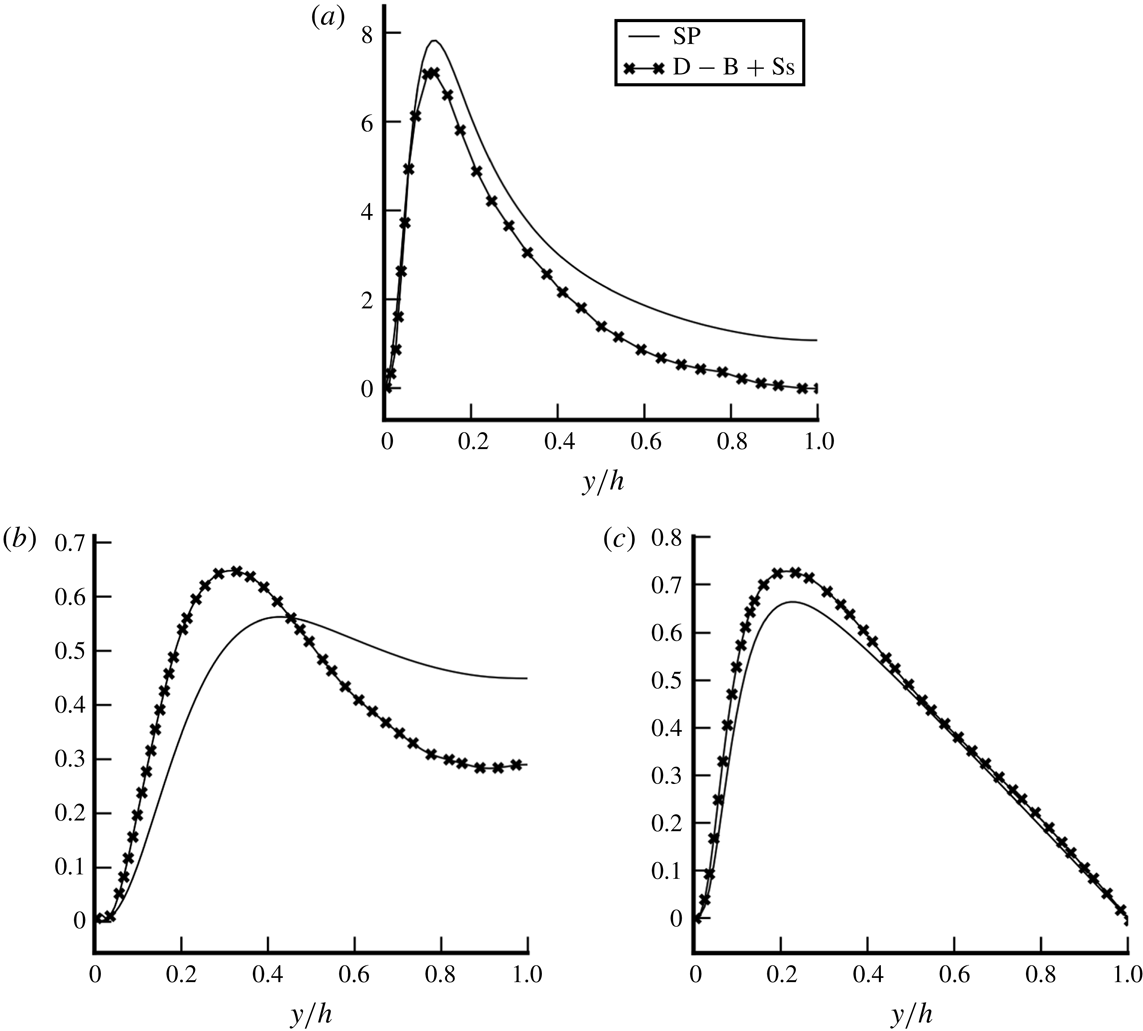
Figures 13(a)–13(c) present the comparison between (4.8) and case SP. For the streamwise component in figure 13(a), it is shown that close to the wall, the shear-induced turbulence is freely developed and the two curves are rather similar. However, a slight decrease of the Reynolds stresses is noticeable at the peak. For the wall-normal component in figure 13(b), the opposite effect is visible. Close to the wall, the Reynolds stresses are increased by the presence of bubbles and the same trend is shown for the cross-correlation
 $\overline{u^{\prime }v^{\prime }}$
in figure 13(c) and for the spanwise component
 $\overline{w^{\prime }w^{\prime }}$
(not shown here). This effect comes from the enhancement of the redistribution process which helps SPT to become more isotropic under the influence of bubbles, taking energy from the streamwise direction and giving it to transverse components. This effect has already been observed by Lance, Marie & Bataille (Reference Lance, Marie and Bataille1991). They show that bubbles reinforce the tendency towards SPT isotropy because the liquid eddies are stretched by the bubbles.
For the streamwise component in figure 13(a), moving from the wall to the bulk of the channel, a reduction of the Reynolds stresses from
 $10\,\%$
to total destruction is observed. Indeed, case SP reaches a finite value at the centre of the channel whereas the SPT in the presence of bubbles reaches zero for case
 $D$
–
 $B$
–
 $Ss$
. A relatively similar process happens in figure 13(b) where the reduction of the wall-normal component of SPT in the bulk is clearly apparent for
 $\overline{v^{\prime }v^{\prime }}$
(the same trend is observed for
 $\overline{w^{\prime }w^{\prime }}$
). This strong reduction of the Reynolds stresses in the bulk can be interpreted as a modulation of the diffusion process by bubbles acting as a shield. However, this hypothesis requires a deeper analysis of turbulent statistics (see § 5) in order to adjudicate on the modulation of SPT. On the other hand, the cross-correlation shown in figure 13(c) behaves differently from diagonal components with almost identical profiles for
 $y/h>0.4$
indicating that the cross-correlation is not affected by the presence of bubbles.
5 Analysis and modelling of the Reynolds stress transport equation
In § 4, we saw that our cases are especially suitable to study BIF and SPT. After the forces, turbulence is the second model required to accurately predict momentum and velocities in two-phase flows. Turbulence predictions are highly empirical because of the lack of knowledge about BIF. Many authors use single-phase modelling extended to two-phase flows by the addition of a specific source term for turbulent kinetic energy and/or dissipation, suggesting that BIF and SPT are statistically independent and that WIF and WIT have features similar to SPT itself (Hosokawa & Tomiyama Reference Hosokawa and Tomiyama2013; Colombo & Fairweather Reference Colombo and Fairweather2015; Vaidheeswaran & Hibiki Reference Vaidheeswaran and Hibiki2017). Besides, there is no consensus about the modelling of these additional terms. As more applications have appeared, a greater variety of models has emerged (see table 5 in the review by Vaidheeswaran & Hibiki (Reference Vaidheeswaran and Hibiki2017)). Thanks to bubble swarm studies (Riboux & Legendre Reference Riboux and Legendre2013; Amoura et al. Reference Amoura, Besnaci and Risso2017; Risso Reference Risso2018), the features of BIF are better understood so that one of the most important questions remaining is the interaction between BIF and SPT. In this section, in addition to the observations made in § 4, the impact of SPT on BIF is investigated. Moreover, in agreement with the demonstration of § 4, BIF in our cases is exclusively comprised of WIF. Several features of WIF are then studied for the purpose of turbulence modelling.
5.1 Transport equation for the Reynolds stress tensor
5.1.1 Physical meaning of the equations
One important characteristic of BIF is the strong anisotropy of the phenomenon. Then, the study of the transport equation for the Reynolds stress tensor is essential and standard
 $k$
–
 $\unicode[STIX]{x1D716}$
models, linear eddy viscosity or Boussinesq approximations are not enough to model two-phase flows. At statistical equilibrium, this transport equation is (Morel Reference Morel2015):
 $$\begin{eqnarray}\displaystyle & & \displaystyle \underbrace{\unicode[STIX]{x1D6FC}_{l}R_{l,ib}\frac{\unicode[STIX]{x2202}\overline{u_{l,j}}^{l}}{\unicode[STIX]{x2202}x_{b}}+\unicode[STIX]{x1D6FC}_{l}R_{l,jb}\frac{\unicode[STIX]{x2202}\overline{u_{l,i}}^{l}}{\unicode[STIX]{x2202}x_{b}}}_{-\unicode[STIX]{x1D617}_{ij}}=\underbrace{\unicode[STIX]{x1D6FC}_{l}\overline{\frac{P_{l}^{\prime }}{\unicode[STIX]{x1D70C}_{l}}\left(\frac{\unicode[STIX]{x2202}u_{l,i}^{\prime }}{\unicode[STIX]{x2202}x_{j}}+\frac{\unicode[STIX]{x2202}u_{l,j}^{\prime }}{\unicode[STIX]{x2202}x_{i}}\right)}^{l}}_{\unicode[STIX]{x1D719}_{ij}}\underbrace{-2\unicode[STIX]{x1D6FC}_{l}\frac{\unicode[STIX]{x1D707}_{l}}{\unicode[STIX]{x1D70C}_{l}}\overline{\frac{\unicode[STIX]{x2202}u_{l,i}^{\prime }}{\unicode[STIX]{x2202}x_{b}}\frac{\unicode[STIX]{x2202}u_{l,j}^{\prime }}{\unicode[STIX]{x2202}x_{b}}}^{l}}_{\unicode[STIX]{x1D716}_{ij}}\nonumber\\ \displaystyle & & \displaystyle \quad \underbrace{-\frac{\unicode[STIX]{x2202}}{\unicode[STIX]{x2202}x_{b}}(\unicode[STIX]{x1D6FC}_{l}\overline{u_{l,i}^{\prime }u_{l,j}^{\prime }u_{l,b}^{\prime }}^{l}-\unicode[STIX]{x1D708}_{l}\frac{\unicode[STIX]{x2202}\unicode[STIX]{x1D6FC}_{l}\unicode[STIX]{x1D619}_{l,ij}}{\unicode[STIX]{x2202}x_{b}}+\frac{\unicode[STIX]{x1D6FC}_{l}}{\unicode[STIX]{x1D70C}_{l}}(\overline{P_{l}^{\prime }u_{l,i}^{\prime }}^{l}\unicode[STIX]{x1D6FF}_{bj}+\overline{P_{l}^{\prime }u_{l,b}^{\prime }}^{l}\unicode[STIX]{x1D6FF}_{ib}))}_{\unicode[STIX]{x1D60B}_{ij}}\nonumber\\ \displaystyle & & \displaystyle \quad \underbrace{-\frac{1}{\unicode[STIX]{x1D70C}_{l}}\overline{(P_{l}^{\prime }u_{l,j}^{\prime }n_{i}+P_{l}^{\prime }u_{l,i}^{\prime }n_{j})\unicode[STIX]{x1D6FF}^{i}}^{l}+\unicode[STIX]{x1D708}_{l}\left[\frac{\unicode[STIX]{x2202}}{\unicode[STIX]{x2202}x_{b}}(\overline{u_{l,i}^{\prime }u_{l,j}^{\prime }n_{b}\unicode[STIX]{x1D6FF}^{i}}^{l})+\overline{\frac{\unicode[STIX]{x2202}u_{l,i}^{\prime }u_{l,j}^{\prime }}{\unicode[STIX]{x2202}x_{b}}n_{b}\unicode[STIX]{x1D6FF}^{i}}^{l}\right]}_{\unicode[STIX]{x1D72B}_{ij}}\;.\end{eqnarray}$$
Previously, Ilic (Reference Ilic2006) and Santarelli et al. (Reference Santarelli, Roussel and Fröhlich2016) have conducted studies for the kinetic energy transport equation. On the basis of their works, the present study is, to the best of our knowledge, the first attempt to leverage DNS data of two-phase flow in order to access the transport equation of the full Reynolds stresses. The production term
 $\unicode[STIX]{x1D617}_{ij}$
corresponds to an energy transfer between the mean kinetic energy and the turbulent kinetic energy. In the context of single-phase channel flows, it is the energy injected at large scales owing to local shear. In two-phase flows, it is expected to exhibit a behaviour similar to that of single-phase flows even if the presence of bubbles can lead to a stronger shear due to the flattening effect (see Colin et al.
Reference Colin, Fabre and Kamp2012).
 $\unicode[STIX]{x1D60B}_{ij}$
is a conservative operator known to diffuse the energy in the flow. Classically, it is split into turbulent, pressure and molecular diffusions. The impact of bubbles on these terms is still unknown by the community. The redistribution term
 $\unicode[STIX]{x1D719}_{ij}$
corresponds to a turbulent energy transfer which redistributes energy between the components through fluctuations in pressure. Lance et al. (Reference Lance, Marie and Bataille1991) show that the redistribution is impacted by the bubbles which reinforce the tendency towards SPT isotropy by stretching the liquid eddies. The dissipation
 $\unicode[STIX]{x1D716}_{ij}$
corresponds to an energy transfer from turbulent kinetic energy to internal energy. This mechanism is also affected by the presence of bubbles, because of the wake structure. Indeed, close to the interface, dissipation strongly increases. Lastly, the interfacial production
 $\unicode[STIX]{x1D6F1}_{ij}$
(which does not exist in single-phase flow) corresponds to an energy transfer between the liquid turbulent kinetic energy and interfacial energy. Classically, it is interpreted as the energy injected at the bubble scale due to the work of the drag force (see Morel Reference Morel2015). It is responsible for the strong anisotropy of two-phase flow turbulence. All these physical mechanisms require a detailed analysis. The aim of this section is to show the complexity of BIF and its interaction with the classical SPT. Except for
 $\unicode[STIX]{x1D6F1}_{ij}$
, all the terms of (5.1) are directly measured numerically. As already argued for the interfacial forces, the interfacial production
 $\unicode[STIX]{x1D6F1}_{ij}$
is also linked to interfacial quantities so that its direct evaluation would lead to significant numerical errors. Instead,
 $\unicode[STIX]{x1D6F1}_{ij}$
is evaluated as the residue of (5.1). Validation of the numerical evaluation of the other terms is achieved by computing the residual of (5.1) on the reference single-phase flow simulation. The numerical residue is below
 $2\,\%$
of the maximal production.
Contributions to the Reynolds stress budget (5.1) for cases D and SP versus the wall-normal coordinate. The colour identifies the terms of the Reynolds stress transport equation (see electronic version). Solid line refers to the single-phase case and markers corresponds to the deformable case.

Averaged terms of (5.1) projected onto the
 $(x,x)$
component: (a) case B; (b) case Ss. The colour identifies the terms of the Reynolds stress transport equation (see electronic version). Empty circles refer to case B whereas small discs correspond to case Ss.

5.1.2 Analysis of the total Reynolds stress transport equation
The terms of (5.1) are shown in figure 14 for cases D and SP and in figure 15 for cases B and Ss. First of all, the zero residue of case SP validates the implementation of statistical measurement. The comparison of cases D and SP in figure 14(a) for the streamwise component shows remarkably well two different areas in the flow. Close to the wall, production
 $\unicode[STIX]{x1D617}_{ij}$
, dissipation
 $\unicode[STIX]{x1D716}_{ij}$
and diffusion
 $\unicode[STIX]{x1D60B}_{ij}$
(but not redistribution
 $\unicode[STIX]{x1D719}_{ij}$
) are rather similar between the two cases so that physical mechanisms are essentially similar to SPT. On the contrary, in the bulk of the channel, single-phase operators tend to zero while interfacial production increases to reach a plateau. At
 $y/h=1$
, the interfacial production is balanced solely by dissipation and redistribution. On the other components of the Reynolds stress tensor, differences are more pronounced. Even close to the wall, terms in case D are larger than for SP. Indeed, a larger amount of turbulent fluctuation is redistributed from component
 $(x,x)$
to other components (as shown by the negative value of
 $\unicode[STIX]{x1D719}_{ij}$
in figure 14(a) and its positive value in figure 14
b or 14
d). Even though the magnitude of
 $\unicode[STIX]{x1D719}_{ij}$
or
 $\unicode[STIX]{x1D716}_{ij}$
is different between SP and D in figures 14(b)–14(d), tendencies across the channel are similar.
For cases B and Ss, only the axial component has been plotted in figures 15(a) and 15(b) because the other components behave similarly. The very strong variations observed around
 $y/h=0.165$
located at the end of the small bubble layer are due to the very sharp transition between the two regimes. To the left of this transition, figures 15(a) and 15(b) are very similar, confirming almost identical flow properties. For case B whose fluctuations are purely due to BIF, figure 15(a) confirms that the interfacial production of turbulent kinetic energy and the redistribution process play important roles in determining the magnitude of
 $\unicode[STIX]{x1D619}_{ij}$
whereas the diffusion is negligible.
5.2 Interaction between SPT and BIF
In § 4, an interaction between SPT and BIF has been brought to light. Furthermore, an innovative methodology has been proposed in § 4.1 for an analysis of this interaction based on cases Ss (small spherical bubbles), B (bidisperse), D (deformable bubbles) and SP (single phase). This process allows to compare the case SP with the SPT part of case D (4.8) and a reduction of the turbulent kinetic energy has been found. The goal of the section is to use this methodology to understand the governing mechanisms involved in this reduction through the analysis of the Reynolds stress transport equation. The decomposition of the Reynolds stresses into SPT and BIF implies the decomposition of the Reynolds stress transport equation such as, at the statistical steady state
 $$\begin{eqnarray}\displaystyle & \displaystyle 0=\unicode[STIX]{x1D719}_{ij}^{SPT}+\unicode[STIX]{x1D716}_{ij}^{SPT}+\unicode[STIX]{x1D60B}_{ij}^{SPT}+\unicode[STIX]{x1D617}_{ij}^{SPT}+\unicode[STIX]{x1D6F1}_{ij}^{SPT}, & \displaystyle\end{eqnarray}$$
 $$\begin{eqnarray}\displaystyle & \displaystyle 0=\unicode[STIX]{x1D719}_{ij}^{BIF}+\unicode[STIX]{x1D716}_{ij}^{BIF}+\unicode[STIX]{x1D60B}_{ij}^{BIF}+\unicode[STIX]{x1D617}_{ij}^{BIF}+\unicode[STIX]{x1D6F1}_{ij}^{BIF}, & \displaystyle\end{eqnarray}$$
where
 $\unicode[STIX]{x1D713}^{SPT}+\unicode[STIX]{x1D713}^{BIF}=\unicode[STIX]{x1D713}$
with
 $\unicode[STIX]{x1D713}\in [\unicode[STIX]{x1D719},\unicode[STIX]{x1D716},D,P,\unicode[STIX]{x1D6F1}]$
. The methodology presented in § 4.1 has been formulated for the Reynolds stresses but it is applicable to each term of (5.1). Thus, the equivalent of (4.7) and (4.8) for
 $\unicode[STIX]{x1D713}\in [\unicode[STIX]{x1D719},\unicode[STIX]{x1D716},D,P,\unicode[STIX]{x1D6F1}]$
is:
 $$\begin{eqnarray}\displaystyle & \displaystyle \unicode[STIX]{x1D713}_{D}^{BIF}=\unicode[STIX]{x1D713}_{B}-\unicode[STIX]{x1D713}_{Ss}, & \displaystyle\end{eqnarray}$$
 $$\begin{eqnarray}\displaystyle & \displaystyle \unicode[STIX]{x1D713}_{D}^{SPT}=\unicode[STIX]{x1D713}_{D}-(\unicode[STIX]{x1D713}_{B}-\unicode[STIX]{x1D713}_{Ss}). & \displaystyle\end{eqnarray}$$
Some of these terms are negligible. For instance, no interfacial production of SPT
 $\unicode[STIX]{x1D6F1}_{ij}^{SPT}$
and no classical production of BIF
 $\unicode[STIX]{x1D617}_{ij}^{BIF}$
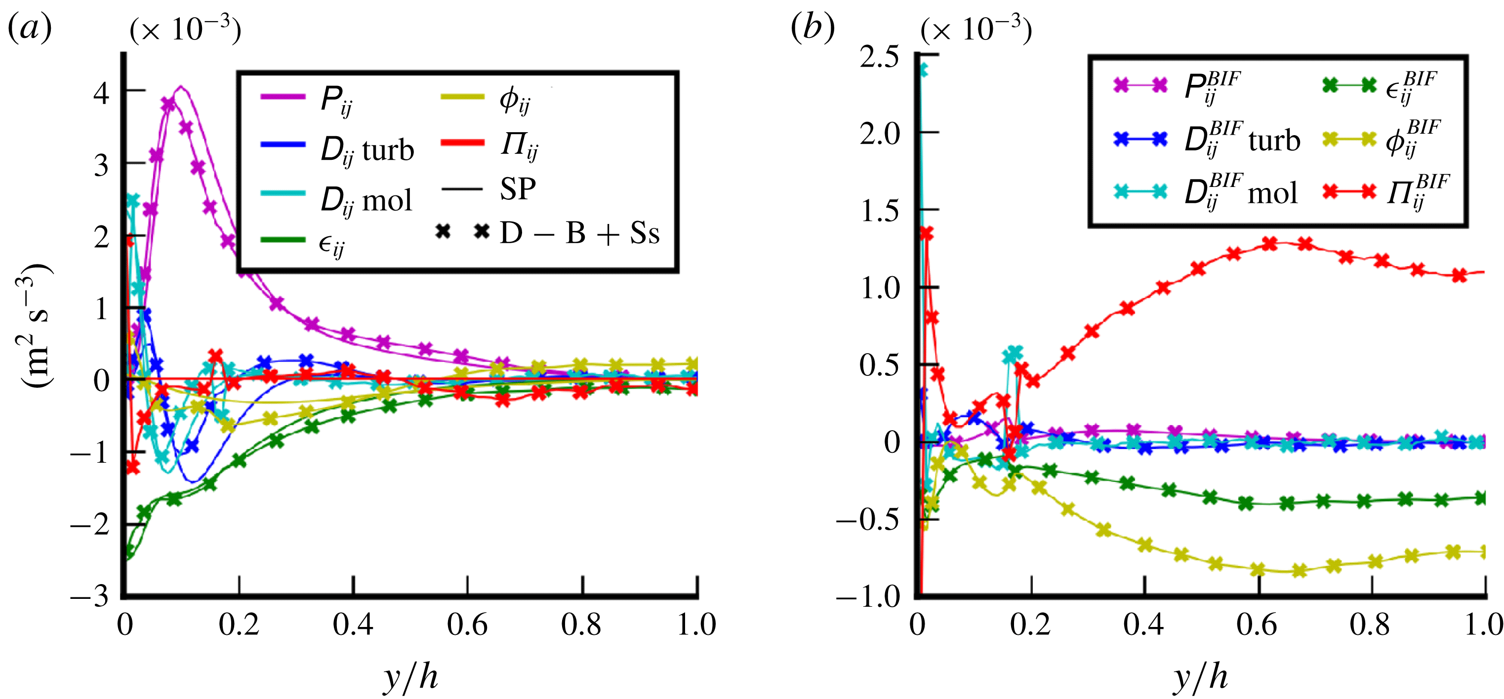
are expected. In figure 16, the terms of (5.2) and (5.3) are plotted and the deviation from zero of
 $\unicode[STIX]{x1D617}_{ij}^{BIF}$
and
 $\unicode[STIX]{x1D6F1}_{ij}^{SPT}$
gives an estimate of the error of this methodology, which appears to be really satisfactory. In figure 16(a), the comparison between
 $\unicode[STIX]{x1D713}_{D}^{SPT}$
given by (5.5) and
 $\unicode[STIX]{x1D713}_{SP}$
is shown in order to understand the impact of bubbles on SPT. Owing to the remarkable similarity between the production terms (
 $\unicode[STIX]{x1D617}_{ij}$
) in this figure, the difference in turbulent kinetic energy cannot be linked to the flattening effect of the velocity profile due to bubbles (as identified in some experiments by Colin et al. (Reference Colin, Fabre and Kamp2012)) because mean velocity gradients are essential in the construction of the production term. In addition, dissipation (
 $\unicode[STIX]{x1D716}_{ij}$
) is rather similar in both cases hence showing no significant modulation by the bubbles even though some effect could be expected due to an increased dissipation in the wakes as in any boundary layer. On the other hand, diffusion presents substantial differences. Both turbulent (
 $\unicode[STIX]{x1D60B}_{ij}$
turb) and molecular (
 $\unicode[STIX]{x1D60B}_{ij}$
mol) diffusion are stronger in the SP case (pressure diffusion is negligible). This means that the bubbles act as a screen on turbulence streaks and prevent the diffusion of the turbulent structures to the bulk of the channel. This interpretation is aligned with the results presented in § 4 where differences between the two cases have been found to be smaller close to the wall. Indeed, the turbulence in the wall boundary layer is ruled by the balance between production and dissipation whereas in the bulk, the diffusion impact becomes significant. Bubbles also act for an increase of the redistribution (
 $\unicode[STIX]{x1D719}_{ij}$
) leading to a more isotropic SPT. This result explains the SPT increase with the presence of bubbles in the wall region for the wall-normal component in figure 13(b). As previously mentioned, this effect has already been observed by Lance et al. (Reference Lance, Marie and Bataille1991). They show that bubbles reinforce the tendency of SPT towards isotropy because the liquid eddies are stretched by the bubbles. This physical coherence between several analyses presented in this paper gives a good confidence in these results. For future work, based on DNS data and theoretical aspects, diffusion and redistribution models for single-phase turbulence will be investigated to take into account the presence of bubbles. For the redistribution, Lance et al. (Reference Lance, Marie and Bataille1991) have already proposed a model to take into account this effect, but to the best of our knowledge, no study has been performed on the modulation of the diffusion.


5.3 WIF modelling
The previous section focused on the analysis of the SPT reduction based on (5.2) and (5.5). This section proposes to study BIF through (5.3) and (5.4). The interpretation of (5.3) is not straightforward. In the present case, BIF is comprised of WIF only, which corresponds to non-turbulent fluctuations due to coherent structures around bubbles. WIF does not present the chaotic features leading to an energy cascade and thus the interpretation of terms such as dissipation or redistribution should be undertaken carefully and the understanding of these notions should evolve in order to break free from the single-phase paradigm. The Reynolds stress transport equation for case B (figure 15
a) shows that WIF proceeds from the balance between interfacial production, redistribution and dissipation. Even for locations where
 $\unicode[STIX]{x1D735}\unicode[STIX]{x1D6FC}_{v}\neq 0$
, the diffusion does not occur (see figure 16
b). This observation is in agreement with WIF features. Indeed, a wake does not ‘diffuse’ into the flow; it always remains located behind a bubble because the dissipation acts quickly so that fluctuations do not have time to diffuse. As long as bubbles are distributed rather homogeneously (
 $\unicode[STIX]{x1D735}\unicode[STIX]{x1D6FC}_{v}\approx 0$
), the gradient of the mean liquid velocity remains small (
 $\unicode[STIX]{x1D735}\overline{u_{l}}\approx 0$
) and the classical production term is then negligible. Eventually, the transport (5.3) for WIF reduces to (see figure 16
b):
 $$\begin{eqnarray}0=\unicode[STIX]{x1D6F1}_{ij}^{WIF}+\unicode[STIX]{x1D719}_{ij}^{WIF}+\unicode[STIX]{x1D716}_{ij}^{WIF}.\end{eqnarray}$$
The following sections provide some insight into the contributions to this equation and propose models for them.
5.3.1 Interfacial production
In figures 14(b) and 14(d), negative interfacial production terms are found. This result is unexpected. Indeed, turbulence modulation usually manifests itself through dissipation or diffusion terms but a negative interfacial production was not expected. Moreover, the interfacial production is often related to the work of the drag force which is zero in the cross-flow directions so that:
 $$\begin{eqnarray}\displaystyle \unicode[STIX]{x1D6F1}_{ij}=\unicode[STIX]{x1D6F1}_{11}\unicode[STIX]{x1D6FF}_{1i}\unicode[STIX]{x1D6FF}_{1j}. & & \displaystyle\end{eqnarray}$$
However, one may wonder whether the difference between the direct evaluation of
 $\unicode[STIX]{x1D6F1}_{ij}$
and this classical assumption comes from the assumption itself or from a numerical error. Indeed, as mentioned previously, the interfacial production is estimated as the residue of (5.1) excluding
 $\unicode[STIX]{x1D6F1}_{ij}$
but measurement of the redistribution term leads to an error which is propagated to the residue. Redistribution is calculated on all cells weighted by the liquid indicator function. The pressure on interfacial cells is an average between liquid and vapour pressures weighted by the phase indicator function. Because of the pressure jump at the interface, the measurement of interfacial terms involving pressure is biased. Thus, the same error can happen on the pressure diffusion term, but in the present case, its global contribution is negligible. A specific procedure could be investigated in future work to prevent numerical errors due to the estimation of redistribution (see Santarelli et al.
Reference Santarelli, Roussel and Fröhlich2016). Meanwhile, the separation of numerical and modelling errors in the estimate of
 $\unicode[STIX]{x1D6F1}_{ij}$
is impossible. As a consequence, (5.7) will be admitted in the following sections as a modelling hypothesis. Then, it is necessary to identify the interfacial production
 $\unicode[STIX]{x1D6F1}_{ij}$
and the redistribution
 $\unicode[STIX]{x1D719}_{ij}$
without resorting to their definitions. The redistribution will not be estimated directly for the following results but a theoretical reconstruction will be used. The sum of interfacial production and redistribution is estimated at the statistical steady state by:
 $$\begin{eqnarray}\displaystyle \unicode[STIX]{x1D719}_{ij}+\unicode[STIX]{x1D6F1}_{ij} & = & \displaystyle -\unicode[STIX]{x1D617}_{ij}-\unicode[STIX]{x1D60B}_{ij}-\unicode[STIX]{x1D716}_{ij}.\end{eqnarray}$$
Then,
 $\unicode[STIX]{x1D719}_{kk}=0$
(Einstein summation convention) because redistribution does not create nor destroy energy. Thus we have:
 $$\begin{eqnarray}\displaystyle \unicode[STIX]{x1D6F1}_{kk}=-\unicode[STIX]{x1D617}_{kk}-\unicode[STIX]{x1D60B}_{kk}-\unicode[STIX]{x1D716}_{kk}. & & \displaystyle\end{eqnarray}$$
Following the idea of (5.7),
 $\unicode[STIX]{x1D6F1}_{11}$
can be estimated as
 $\unicode[STIX]{x1D6F1}_{kk}$
so that:
 $$\begin{eqnarray}\displaystyle \unicode[STIX]{x1D6F1}_{ij}=(-\unicode[STIX]{x1D617}_{kk}-\unicode[STIX]{x1D60B}_{kk}-\unicode[STIX]{x1D716}_{kk})\unicode[STIX]{x1D6FF}_{1i}\unicode[STIX]{x1D6FF}_{1j}. & & \displaystyle\end{eqnarray}$$
Finally, with (5.8), the redistribution is given by:
 $$\begin{eqnarray}\displaystyle \unicode[STIX]{x1D719}_{ij}=-\unicode[STIX]{x1D617}_{ij}-\unicode[STIX]{x1D60B}_{ij}-\unicode[STIX]{x1D716}_{ij}+(\unicode[STIX]{x1D617}_{kk}+\unicode[STIX]{x1D60B}_{kk}+\unicode[STIX]{x1D716}_{kk})\unicode[STIX]{x1D6FF}_{1i}\unicode[STIX]{x1D6FF}_{1j}. & & \displaystyle\end{eqnarray}$$
Thus,
 $\unicode[STIX]{x1D6F1}$
and
 $\unicode[STIX]{x1D719}$
are modelled from
 $P$
,
 $D$
and
 $\unicode[STIX]{x1D716}$
. The comparison between the direct evaluation of redistribution and interfacial production to the model proposed in (5.10) and (5.11) is shown in figure 17 for the three diagonal components of the operators and for the cross-correlation (12). There is no major differences to notice but this model is more convenient for the following physical analysis.
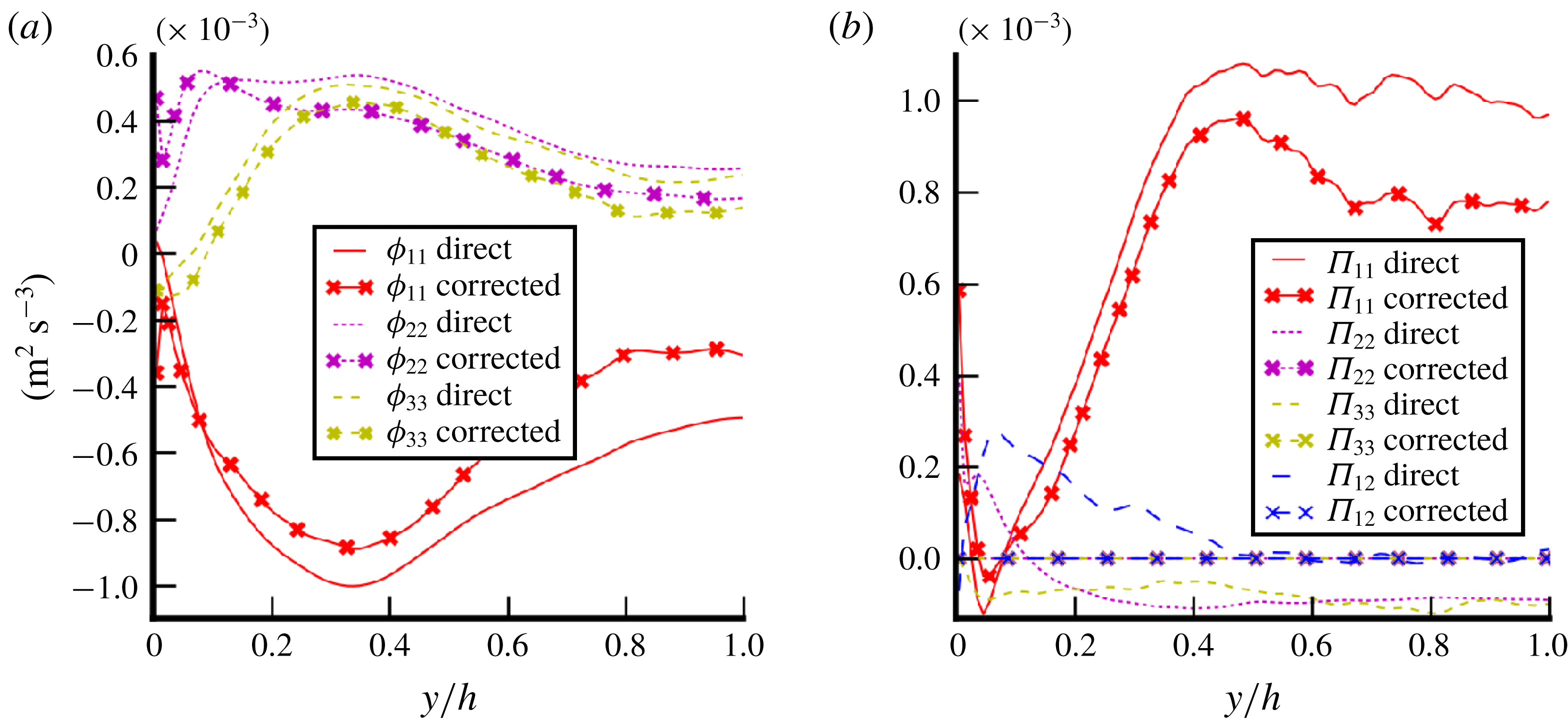
Consensus has been reached in the literature concerning the interfacial production. It is often taken as the work of the drag force such that:
 $$\begin{eqnarray}\unicode[STIX]{x1D6F1}_{ij}=\frac{3}{4d_{b}}\unicode[STIX]{x1D6FC}_{l}C_{D}|u_{r}|^{2}u_{r}\unicode[STIX]{x1D6FF}_{1i}\unicode[STIX]{x1D6FF}_{1j}.\end{eqnarray}$$
Based on this idea, several variations exist (Pfleger & Becker Reference Pfleger and Becker2001; Olmos, Gentric & Midoux Reference Olmos, Gentric and Midoux2003). The drag coefficient
 $C_{D}$
depends on the flow regime but an exact expression is given by the balance of drag with the buoyancy force:
 $$\begin{eqnarray}C_{D}=\frac{4}{3}\frac{\unicode[STIX]{x1D6FC}_{v}d_{b}(\unicode[STIX]{x1D70C}_{v}-\unicode[STIX]{x1D70C}_{l})g}{\unicode[STIX]{x1D70C}_{l}u_{r}^{2}}.\end{eqnarray}$$
In figure 18(b), this model is compared to DNS results. It slightly underpredicts the interfacial production with an error inferior to
 $10\,\%$
. The differences between the work of the drag force and the DNS interfacial source term is caused by (5.12) which derives from (5.1) under several hypotheses (see Morel Reference Morel2015).
5.3.2 Redistribution
WIF is known for being strongly anisotropic because of the averaged contribution of wakes which occurs principally in the longitudinal direction (Amoura et al.
Reference Amoura, Besnaci and Risso2017). The bubble velocity is not purely axial because bubbles are disturbed by transverse forces so that the instantaneous wakes show a slight inclination with respect to the
 $x$
axis (see wakes in figure 11
b). However, this inclination is so small that a huge anisotropy of the flow is expected. The redistribution process is the phenomenon responsible for the energy repartition between components. Basically, the energy is created by the interfacial production on the (
 $x,x$
) component and then a part of this energy is equally redistributed to other directions (see figures 14
b and 14
d for instance). This observation led Hosokawa & Tomiyama (Reference Hosokawa and Tomiyama2013) and Colombo & Fairweather (Reference Colombo and Fairweather2015) to propose a modelling of the redistribution such as:
 $$\begin{eqnarray}\unicode[STIX]{x1D719}_{ij}^{BIF}+\unicode[STIX]{x1D6F1}_{ij}^{BIF}=\left(\begin{array}{@{}ccc@{}}\frac{1}{2} & 0 & 0\\ 0 & \frac{1}{4} & 0\\ 0 & 0 & \frac{1}{4}\end{array}\right)\unicode[STIX]{x1D6F1}_{11}.\end{eqnarray}$$
This expression has been proposed for BIF in a general sense. For reasons developed previously, a generic model cannot exist for both WIF and WIT together. Based on a purely WIF case, the model is tested in figure 18(a). This figure shows that the redistribution model is satisfactory even if it slightly underpredicts the anisotropy of WIF. Actually, this model has been fitted on cases with additional WIT, expected to be less anisotropic than WIF. This could be part of the reasons for the slight differences. Eventually, for purely WIF conditions, our DNS suggests the following model:
 $$\begin{eqnarray}\unicode[STIX]{x1D719}_{ij}^{WIF}+\unicode[STIX]{x1D6F1}_{ij}^{WIF}=\left(\begin{array}{@{}ccc@{}}\frac{3}{5} & 0 & 0\\ 0 & \frac{1}{5} & 0\\ 0 & 0 & \frac{1}{5}\end{array}\right)\unicode[STIX]{x1D6F1}_{11}.\end{eqnarray}$$
For a case entirely comprised of WIF, a larger amount of energy is carried by the streamwise component (
 $3/5\unicode[STIX]{x1D6F1}_{11}$
against
 $1/2\unicode[STIX]{x1D6F1}_{11}$
). In the model of Colombo & Fairweather (Reference Colombo and Fairweather2015), the addition of WIT is responsible for a more isotropic repartition of energy. The variation of the redistribution (matrix (5.15)) in the region where there is a gradient of void fraction (
 $0.2<y/h<0.5$
) suggests an impact of the void-fraction gradient not included in the model. Nevertheless, the variation of this redistribution matrix with the void fraction is weak (from
 $0.5$
to
 $0.6$
for a void fraction increasing from
 $0\,\%$
to
 $4\,\%$
). This observation is in agreement with the literature where the redistribution matrix is often taken as a constant.


Assessment of dissipation relaxation time model in the purely WIF case (B–Ss) (5.16).

5.3.3 Dissipation
The most challenging part for the modelling of WIF is the dissipation term. The most popular method is to define a relaxation time
 $\unicode[STIX]{x1D70F}$
:
 $$\begin{eqnarray}\unicode[STIX]{x1D70F}=\frac{\unicode[STIX]{x1D619}_{ij}}{\unicode[STIX]{x1D716}_{ij}}.\end{eqnarray}$$
The ratio
 $\unicode[STIX]{x1D619}_{ij}/\unicode[STIX]{x1D716}_{ij}$
is rather independent from the component
 $ij$
(see figure 19) so that
 $\unicode[STIX]{x1D70F}$
can be regarded as a scalar. Rzehak & Krepper (Reference Rzehak and Krepper2013) define the relaxation time as the lifetime of turbulent structures (see also Wilcox Reference Wilcox1993). Thus, in the context of pure WIF, the relaxation time can be seen as the time needed to cross the wake. In Rzehak & Krepper (Reference Rzehak and Krepper2013), several definitions are proposed based on different quantities of the flow for BIF in a general sense. They argued that relaxation time can be linked to averaged quantities of bubbles (
 $\unicode[STIX]{x1D70F}=d_{b}/u_{r}$
) or to averaged quantities of the liquid phase (
 $\unicode[STIX]{x1D70F}=k/\unicode[STIX]{x1D716}$
). Cross-definitions have also been proposed but the appropriate relaxation time is still an open question. More definitions are found in Troshko & Hassan (Reference Troshko and Hassan2001) or Pakhomov & Terekhov (Reference Pakhomov and Terekhov2015) for instance. The profusion of models for the relaxation time comes from the fact that a generic model cannot exist for both WIF and WIT together. WIF and WIT are subject to two different relaxation times because of their different natures. Therefore, the model must be adapted, depending on the ratio between WIF and WIT. However, based on the definition of ‘time needed to go through the wake’, the relaxation time for a pure WIF case can be defined as
 $$\begin{eqnarray}\unicode[STIX]{x1D70F}=\frac{L_{w}}{u_{r}},\end{eqnarray}$$
where
 $u_{r}$
is the relative velocity of the bubbles and
 $L_{w}$
is the length of the wake taken as a function of the bubble diameter. In figure 19, diagonal components of the normalized dissipation are plotted and compared to this relaxation time with different values of the wake length from
 $2d_{b}$
to
 $4d_{b}$
. First of all, it confirms that the normalization component per component presents rather similar relaxation times for all the components. No physical explanation could be gathered from our results. Then, a good agreement is found for
 $L_{w}=3$
or
 $4d_{b}$
. In figure 11(b), instantaneous structures of wakes in case B are shown. The length of
 $3d_{b}$
is found to be aligned with the observations. Indeed, in figure 11(b), wakes of large bubbles disappear (transition between green and blue) after approximately
 $3d_{b}$
. Nevertheless, the wake length depends on dimensionless numbers such as the bubble Reynolds number; thus the present value is illustrative but is not expected to be generic. This length should also depend on the void fraction. Indeed, Risso & Ellingsen (Reference Risso and Ellingsen2002) have shown that the decrease of a wake is faster for bubbles in a collective swarm than for an isolated bubble (see also Amoura et al.
Reference Amoura, Roig, Risso and Billet2010). It has to be noticed that the present wake length does not fit with the classical scaling
 $L_{w}=d_{b}/C_{d}$
(Risso et al.
Reference Risso, Roig, Amoura, Riboux and Billet2008). Thus, this wake length estimate is a shortcoming of the present analysis. It should be alleviated by future work dedicated to the quest for a more generic closure.
5.3.4 Algebraic models for WIF
Bringing together (5.6), (5.12), (5.13), (5.15), (5.16) and (5.17), an algebraic closure for the WIF Reynolds stresses is found:
 $$\begin{eqnarray}\unicode[STIX]{x1D619}_{ij}^{WIF}=\left(\begin{array}{@{}ccc@{}}\frac{3}{5} & 0 & 0\\ 0 & \frac{1}{5} & 0\\ 0 & 0 & \frac{1}{5}\end{array}\right)\unicode[STIX]{x1D6FC}_{l}\unicode[STIX]{x1D6FC}_{v}\frac{\unicode[STIX]{x0394}\unicode[STIX]{x1D70C}}{\unicode[STIX]{x1D70C}_{l}}gL_{w}.\end{eqnarray}$$
Another algebraic closure has been proposed by Risso (Reference Risso2016). The reasoning of Risso (Reference Risso2016) is not based on the budget of turbulent kinetic energy but on the wake structure and potential flow around the bubbles. Performing the integration of the velocity field induced by the averaged wake in an infinite domain, he shows that the corresponding Reynolds stress is:
 $$\begin{eqnarray}\unicode[STIX]{x1D619}_{ij}^{wake}=\unicode[STIX]{x1D6FC}_{v}\frac{3u_{r}^{2}L_{w}e^{2}}{16r_{b}^{3}}\left(\begin{array}{@{}ccc@{}}1 & 0 & 0\\ 0 & 0 & 0\\ 0 & 0 & 0\end{array}\right),\end{eqnarray}$$
where
 $e$
is the semi-width of the wake (
 $e\approx 0.2=1.3r_{b}$
in our cases). Then, using the results of Biesheuvel & Wijngaarden (Reference Biesheuvel and Wijngaarden1984), he shows that the Reynolds stress induced by the potential flow around a spherical bubble is:
 $$\begin{eqnarray}\unicode[STIX]{x1D619}_{ij}^{potential}=\unicode[STIX]{x1D6FC}_{v}u_{r}^{2}\left(\begin{array}{@{}ccc@{}}\frac{1}{5} & 0 & 0\\ 0 & \frac{3}{20} & 0\\ 0 & 0 & \frac{3}{20}\end{array}\right).\end{eqnarray}$$
Test of algebraic closure (5.18) for the total kinetic energy (TKE) of BIF for deformable bubbles (case B–Ss) in purely WIF conditions.

The total Reynolds stress
 $\unicode[STIX]{x1D619}_{ij}^{Risso}=\unicode[STIX]{x1D619}_{ij}^{wake}+\unicode[STIX]{x1D619}_{ij}^{potential}$
(5.19)
 $+$
(5.20) is expected to be applicable for bubbles with a purely vertical trajectory. To compare to our case where bubbles are also disturbed by transverse forces, only turbulent kinetic energies (
 $k=\text{tr}(\unicode[STIX]{x1D619}_{ij})$
) are compared. The trace of
 $\unicode[STIX]{x1D619}_{ij}^{Risso}$
is called
 $k_{Risso}$
. The trace of (5.18) is called
 $k_{budget}$
and both are compared to the WIF kinetic energy produced by the deformable bubbles (case B–Ss) in figure 20. Both models underpredict the same kinetic energy for a given
 $L_{w}$
. This is due to the modelling of the interfacial production based on the work of the drag force (see figure 18
b). For
 $y<0.2$
, the model shows a peculiar behaviour due to the void-fraction reconstruction as
 $\unicode[STIX]{x1D6FC}_{D}=\unicode[STIX]{x1D6FC}_{B}-\unicode[STIX]{x1D6FC}_{Ss}$
which should not be included in the discussion. Further away from the wall, the two models give reasonable results. Besides, the validity of this new model is currently limited to specific physical configurations (drag–buoyancy-driven flow, small gravity conditions). It has been developed only for
 $y/h>0.2$
so there is no evaluation of its capabilities in the near-wall region where the wakes could be disturbed by the no-slip boundary condition or by the large amount of SPT. More importantly, the model depends on a wake length
 $L_{w}$
which in turn possibly evolves with the Eötvös number, the bubble Reynolds number and the void fraction. Finally, further analyses are needed in different conditions to extend the closure validity. Explicit testing and validation of the model against experimental or numerical data are also necessary.
5.3.5 Discussion on two-phase turbulence modelling
After carrying out these analyses on SPT modulation and on the WIF transport equation, a thorough analysis of the turbulence has been completed and the first proposal for an innovative two-phase turbulence model can be sketched as follows:
 $$\begin{eqnarray}\displaystyle & \displaystyle \unicode[STIX]{x1D619}_{ij}=\unicode[STIX]{x1D619}_{ij}^{SPT}+\unicode[STIX]{x1D619}_{ij}^{WIT}+\unicode[STIX]{x1D619}_{ij}^{WIF}, & \displaystyle\end{eqnarray}$$
 $$\begin{eqnarray}\displaystyle & \displaystyle \frac{D\unicode[STIX]{x1D619}_{ij}^{SPT}}{Dt}=\unicode[STIX]{x1D617}_{ij}^{SPT}+\unicode[STIX]{x1D719}_{ij}^{SPT}+\unicode[STIX]{x1D716}_{ij}^{SPT}+\unicode[STIX]{x1D60B}_{ij}^{SPT}, & \displaystyle\end{eqnarray}$$
 $$\begin{eqnarray}\displaystyle & \displaystyle \frac{D\unicode[STIX]{x1D619}_{ij}^{WIT}}{Dt}=\unicode[STIX]{x1D6F1}_{ij}^{WIT}+\unicode[STIX]{x1D719}_{ij}^{WIT}+\unicode[STIX]{x1D716}_{ij}^{WIT}+\unicode[STIX]{x1D60B}_{ij}^{WIT}, & \displaystyle\end{eqnarray}$$
 $$\begin{eqnarray}\displaystyle & \displaystyle \unicode[STIX]{x1D619}_{ij}^{WIF}=\left(\begin{array}{@{}ccc@{}}\frac{3}{5} & 0 & 0\\ 0 & \frac{1}{5} & 0\\ 0 & 0 & \frac{1}{5}\end{array}\right)\unicode[STIX]{x1D6FC}_{l}\unicode[STIX]{x1D6FC}_{v}\frac{\unicode[STIX]{x0394}\unicode[STIX]{x1D70C}}{\unicode[STIX]{x1D70C}_{l}}gL_{w}, & \displaystyle\end{eqnarray}$$
where
 $\unicode[STIX]{x1D619}_{ij}^{SPT}$
is the single-phase turbulence classically modelled with a Reynolds stress model (Launder, Reece & Rodi Reference Launder, Reece and Rodi1975; Speziale, Sarkar & Gatski Reference Speziale, Sarkar and Gatski1991). The present study has shown that the redistribution tensor
 $\unicode[STIX]{x1D719}_{ij}^{SPT}$
is disturbed by the presence of bubbles in accordance with the study of Lance et al. (Reference Lance, Marie and Bataille1991). Additionally, diffusion is reduced by the near-wall bubble layer. In the long term, the characteristic scale in the modelling of
 $\unicode[STIX]{x1D60B}_{ij}^{SPT}$
should also be modified in order to take into account the impact of bubbles. Concerning the bubble-induced fluctuations, the present study was focused on finding an algebraic closure for the WIF as proposed in (5.24). The next step is to develop a transport equation dedicated to the WIT related to wake instabilities and interactions.
6 Conclusion and prospects
Five DNS calculations have been performed for a vertical bubbly flow at
 $Re_{\unicode[STIX]{x1D70F}}=127$
and analysed through budget equations of the momentum or Reynolds stresses in order to improve our understanding of such flows. These cases have been compared with both single-phase flow (Vreman & Kuerten Reference Vreman and Kuerten2014) and two-phase flow (Lu & Tryggvason Reference Lu and Tryggvason2008) references and confidence in the results has been reinforced by additional mesh convergence tests on isolated bubbles. Cases have been studied in low gravity conditions such that bubble-induced fluctuations (BIF) are related only to wake-induced fluctuations (WIF). The momentum budget brings into light the influence of surface tension on wall-normal interfacial forces and thus on bubble dispersion. However, further work is necessary to enable a physical interpretation of the impact of surface tension on bubble migration even if its importance in the momentum budget in the direction of migration is demonstrated. Concerning the budget of the Reynolds stresses, the four complementary cases (small spherical bubbles, large deformable bubbles, bidisperse and single-phase cases) are well suited to studying the modulation of SPT (single-phase turbulence) and WIF mechanisms. A statistical dependence between BIF and SPT has been observed, revealing weaknesses in the classical way in which pseudoturbulence and perturbations to standard single-phase turbulence are modelled. Moreover, it has been shown that this SPT reduction is due to an alteration of the diffusion from the wall to the bulk of the channel because of the presence of bubbles. An increase of the redistribution leading to a more isotropic SPT has been observed as well. In the future, SPT modelling should take into account these phenomena. Finally, a physical interpretation of the WIF transport equation has been proposed through the investigation of interfacial production, redistribution and dissipation. The relaxation time responsible for the dissipation was found to be related to the wake length. Two algebraic closures based on physical assertions for the Reynolds stresses have then been tested. The results are encouraging, further analyses are needed at different bubbles Reynolds numbers or void fractions to extend the closure validity (in particular to assess the possible dependency of the characteristic length scale of the wake); further efforts are required to actually estimate the capabilities of the model. In addition, investigations of mechanisms in the near-wall region would be valuable to improve the applicability of the model. Otherwise, the DNS database is now available for further analysis. (See http://triocfd.cea.fr/recherche/modelisation-physique/.)
Acknowledgements
The authors would like to convey their sincere thanks to GENCI and the TGCC and CINES for providing the necessary computational resources to perform DNS calculations. This work was granted access to the HPC resources of TGCC under the allocations X20162B7712 and A0022B07712 made by GENCI.