II. COMPARISON OF PROJECTED CONTACT AREAS FOR CONICAL AND BERKOVICH INDENTATIONS

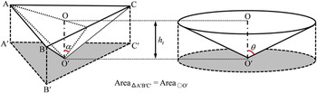
Figure 1 shows a triangular pyramidal indenter, and its equivalent axisymmetric conical indenter giving the same projected area at equal depth; Area of triangle A′B′C′ is equal to area of circle O′. The centerline-to-face angle of the triangular pyramidal indenter (α) and the corresponding half-included angle of the conical indenter (θ) are related to each other via

(3) $$\theta = {\tan ^{ - 1}}\left( {\sqrt {{{3\sqrt 3 } \over \pi }} \tan \alpha } \right)\quad {\rm{.}}$$

FIG. 1.

Schematic diagram of a triangular pyramidal indenter with the indenter angle α, and its equivalent axisymmetric conical indenter with the indenter angle θ giving the same projected area.

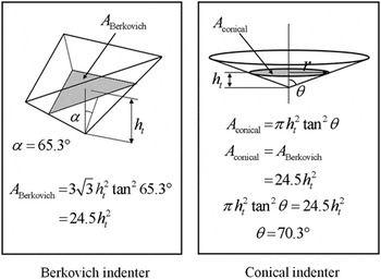
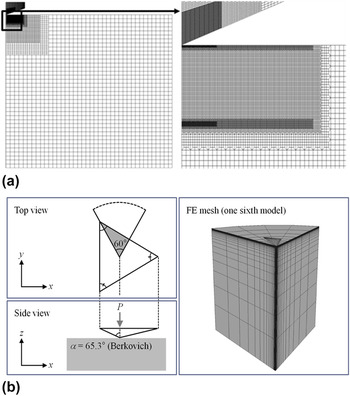
The equivalent cone angle of the Berkovich indenter (α = 65.3°) is θ = 70.3° (Fig. 2). For the same indentation depth, we compare projected contact areas for conical and Berkovich indentations to see whether the theoretical statement is in accordance with FE results. Details on acquiring the contact area will be provided later. Figure 3 shows the finite element model for both indenters. For the FE model for conical indentation, 4-node axisymmetric elements (CAX4, Abaqus ²⁴ ) are used. Considering the symmetry of the triangular pyramidal indenter, only one sixth of indenter and specimen are modeled using three-dimensional 6-node (C3D6, Abaqus ²⁴ ) and 8-node (C3D8, Abaqus ²⁴ ) elements. The indenter is made of tungsten carbide (WC; E _I = 537 GPa and ν_I = 0.24). We adopted the same minimum element size of FE model for conical and triangular pyramidal indentation. In simulations with WC indenters, we consider only elastic deformation of indenter. All simulations are performed to a maximum indentation depth of h _max = 0.05 mm.

FIG. 2.

Schematic of two indenters with the same projected contact area.

FIG. 3.

Overall mesh design (a) using axisymmetric conical indenter and (b) 1/6 triangular pyramidal indenter (α = 65.3°; Berkovich).

The material is assumed to obey the following piecewise power law suggested by Rice and Rosengren ^{Reference Rice and Rosengren25}

(4) $${{\varepsilon _{\rm{t}} } \over {\varepsilon _0 }} = \left\{ {\matrix{\!\!\!\!\!\!\!\!\!\!\!\!\!\!\!\!\!\!\!\!\!\!\!\!\! {{\sigma \over {\sigma _0 }}\quad \;\;\,{\rm{for}}\;\sigma \;\le\; \sigma _0 } \cr {\left( {{\sigma \over {\sigma _0 }}} \right)^n \quad {\rm{for}}\;\sigma > \sigma _0 ;1 \;\lt \;n \;\le \;\infty } \cr } } \right.\quad {\rm{,}}$$

where ε₀ (= σ₀/E) is the yield strain, E is the Young's modulus, and σ₀ is the yield strength. Total strain ε_t can be divided into elastic and plastic strain (ε_t = ε_e + ε_p). Hyun et al. ^{Reference Hyun, Kim, Lee and Lee21} (sharp indentation) and Lee et al. ^{Reference Lee, Lee and Pharr26} (spherical indentation) have shown that the influence of friction coefficient f on the load–depth curve is negligible for nonzero f. Qin et al. ^{Reference Qin, Huang, Hwang, Song and Pharr27} further showed that for indenters with high indenter angles friction does not affect the load–depth curve. Since friction coefficient between metals is usually 0.1 ≤ f ≤ 0.4, we use f = 0.2 in this study.

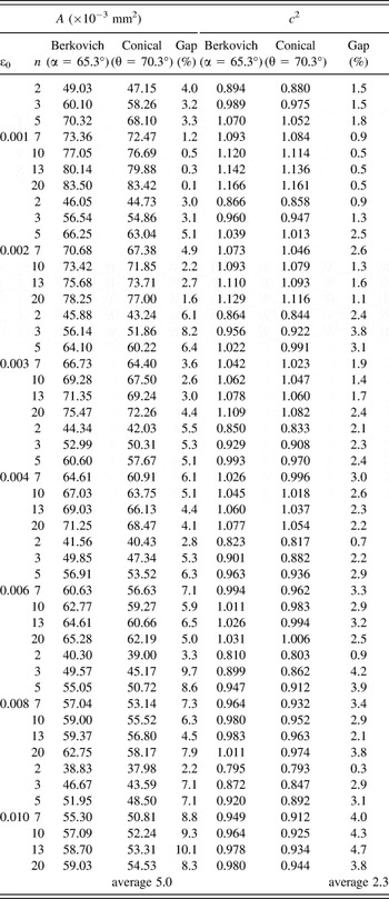
We checked the difference between projected contact areas A for 56 different materials (E = 200 GPa; ε₀ = 0.001, 0.002, 0.003, 0.004, 0.006, 0.008, 0.010; n = 2, 3, 5, 7, 10, 13, 20). Table I shows that the values of A obtained by Berkovich indentation are larger than the values obtained by conical indentation for all the given materials. The average gap between A values increases with increasing ε₀. Our results are consistent with the findings by Shim et al. ^{Reference Shim, Oliver and Pharr22} who reported that conical and Berkovich indenters produce different projected contact areas at equal indentation depths.

TABLE I.

Comparison of A and c ² for two different indenters (E = 200 GPa, h _max = 0.05 mm).

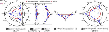
In a fashion equal to Shim et al., ^{Reference Shim, Oliver and Pharr22} Figs. 4(a) and 4(e) provide the projected contact areas at h _max = 0.1 mm for conical and Berkovich indentations of pure elastic and elastic-perfectly-plastic materials (E = 72 GPa, Poisson's ratio ν = 0.17; σ₀ = 5.5 GPa). While for purely elastic indentation, the projected contact area for Berkovich indentation is smaller than that for conical indentation (0.094/0.099 mm² = 94.9%), for elastic-perfectly-plastic indentation, it is larger (0.135/0.128 mm² = 105.5%). Both indenters undergo sink-in for the two materials which are given. More notably, the contact line of Berkovich indenter is not in a plane differently from that of conical indenter. This is illustrated in Figs. 4(b)–4(d) which show the side views of the contact perimeters. Figure 4(b) is the contact lines projected on the rectangle BB′C′C plane of Fig. 1, and Fig. 4(c) is the contact lines for normal view to triangle BO′C of Fig. 1. In Berkovich indentation, the concave appearance of contact impression is caused by further sink-in at the middle of indenter faces than sink-in at edges. It can readily be understood with the 90° clockwise rotation of Fig. 4(c), which results in Fig. 4(d). Nonequal projected contact areas of two indenters and nonplanar contact line of Berkovich indenter are the main sources of different indentation characteristics of two indenters.

FIG. 4.

The plan view and side view of indentation contact geometries in pure elastic material and elastic-perfectly-plastic material.

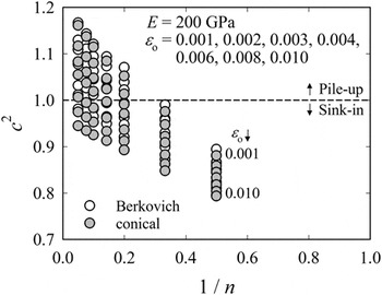
To consider the pile-up/sink-in behavior we introduce the dimensionless parameters c ²|_conical ≡ (h + h _g)/(h _max + h _g), $c_{\left| {{\rm{triangular}}\;{\rm{pyramidal}}} \right.}^2 \equiv \sqrt {{A \mathord{\left/ {\vphantom {A {A_{\rm{t}} }}} \right. \kern-\nulldelimiterspace} {A_{\rm{t}} }}}$ . Here h is the actual indentation depth considering pile-up or sink-in, and h _g is the difference between the depths obtained using conical indenters with zero and finite tip-radius. ^{Reference Lee, Lee and Kim6,Reference Hyun, Kim, Lee and Lee21} A _t is the nominal (theoretical) projected contact area at h _max. In practice, it is very hard to get the projected contact area at maximum load P _max. The key parameter in this study is the actual projected contact area A. To evaluate the actual projected contact area A, we adopt the approach by Hay and Crawford ^{Reference Hay and Crawford28} and take the intersection of the line through the last two surface nodes in contact with the line through the first two nodes not in contact (zero contact pressure) at P _max. For both indenters, c ² is plotted against 1/n in Fig. 5. c ²|_{triangular pyramidal} is always larger than c ²|_conical for all elastic–plastic materials (Table I). For the evaluation of properties by a dual indentation technique, it is therefore necessary to study the triangular pyramidal indenter case separately from the conical indenter case.

FIG. 5.

Comparison of c ² values for two different indenters.

III. CALCULATION OF YOUNG’S MODULUS

From the indentation P–h _t data, Young's modulus can be calculated by ^{Reference Oliver and Pharr29}

(5) $$S = \beta {2 \over {\sqrt \pi }}{E_{\rm{r}}}\sqrt A \quad {\rm{.}}$$

Here S is the contact stiffness; E _r is the effective Young's modulus; and β is a correction factor that depends on the indenter geometry (β_Vickers = 1.012, β_Berk = 1.034). ^{Reference King30} The definition of E _r is

(6) $${1 \over {{E_{\rm{r}}}}} \equiv {{\left( {1 - {\nu ^2}} \right)} \over E} + {{\left( {1 - \mathop {{\nu _{\rm{I}}}}\nolimits^2 } \right)} \over {{E_{\rm{I}}}}}\quad {\rm{.}}$$

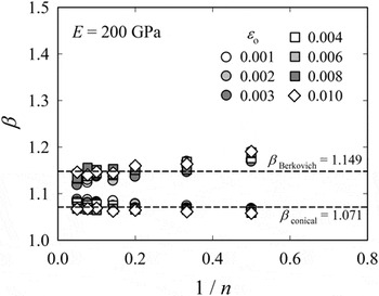
The section regressed to get the contact stiffness S is set to ΔP/P _max = 20%, as in Hyun's study. ^{Reference Hyun, Kim, Lee and Lee21} Hay et al. ^{Reference Hay, Bolshakov and Pharr31} considered the elastic radial displacement and proposed that β is a function of the indenter's half-included angle and Poisson's ratio. Pharr ^{Reference Pharr32} derived β by assuming that the Berkovich indenter can be adequately modeled by a 70.3° cone. Similar to c ², we check β for Berkovich and conical indenters for the same material properties. Figure 6 provides β values obtained for the two indenters. Since the deviation of β from its average is <5%, irrespective of material properties, β can be regarded as a constant. The average β value for Berkovich indentation (β_Berko = 1.149) is 6.8% higher than for conical indentation (β_cone = 1.071). The result is in agreement with Shim et al. ^{Reference Shim, Oliver and Pharr22} who found β_Berko = 1.141–1.158 and β_cone = 1.060–1.072. In this study, we take the average β_Berko = 1.149.

FIG. 6.

β versus 1/n curves for various values of ε₀ with two different indenters.

Young's modulus E can be derived by ^{Reference Oliver and Pharr29}

(7) $$E = {{\left( {1 - {\nu ^2}} \right)S\sqrt \pi {E_{\rm{I}}}} \over {2\beta \sqrt A {E_{\rm{I}}} - \left( {1 - \mathop {{\nu _{\rm{I}}}}\nolimits^2 } \right)S\sqrt \pi }}\quad {\rm{.}}$$

To obtain $\sqrt A$ as a function of ε₀ and n we propose

(8) $$\eqalignb{ &#x0026; {c^2} \equiv \sqrt {{A \mathord{\left/ {\vphantom {A {{A_{\rm{t}}}}}} \right. \kern-\nulldelimiterspace} {{A_{\rm{t}}}}}} = {f^{{\rm{TP}}}}\left( {{\varepsilon _0},n} \right) = f_{1i}^{{\rm{TP}}}\left( {{\varepsilon _0}} \right){n^{ - i}} = \left( {{\kappa _{1ij}}\mathop {{\varepsilon _0}}\nolimits^j } \right){n^{ - i}} \cr &#x0026; \quad\quad\quad\quad\!\! i,j = 0,1,2,3\quad {\rm{.}} \cr}$$

Inserting Eq. (8) into (7) we can write

(9) $$E = {{\left( {1 - {\nu ^2}} \right)S\sqrt \pi {E_{\rm{I}}}} \over {2\beta {c^2}\sqrt {{A_{\rm{t}}}} {E_{\rm{I}}} - \left( {1 - \mathop {{\nu _{\rm{I}}}}\nolimits^2 } \right)S\sqrt \pi }} = {{\left( {1 - {\nu ^2}} \right)S\sqrt \pi {E_{\rm{I}}}} \over {2\beta {f^{{\rm{TP}}}}\left( {{\varepsilon _0},n} \right)\sqrt {{A_{\rm{t}}}} {E_{\rm{I}}} - \left( {1 - \mathop {{\nu _{\rm{I}}}}\nolimits^2 } \right)S\sqrt \pi }}\quad {\rm{.}}$$

IV. CHARACTERISTICS OF INDENTATION DEFORMATION

A. Characteristics of load–depth curves

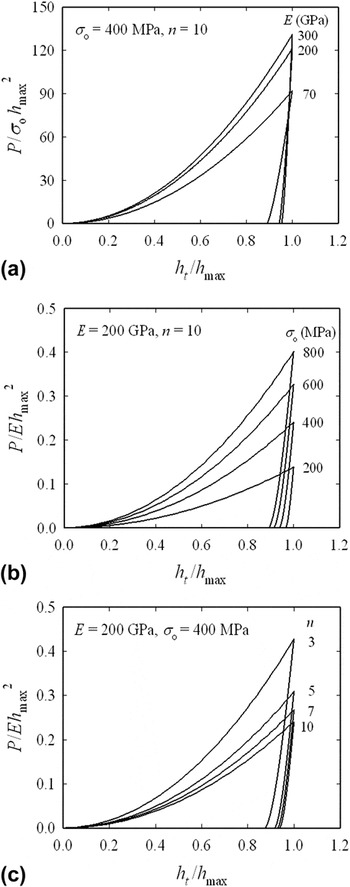
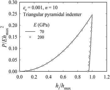
Figure 7 shows the effects of E, σ₀, and n on the P–h _t curves for Berkovich indentation. The load P increases with E and σ₀, but decreases with n for equal h _t. Note that unloading curves vary sensitively with E. While all the material properties affect the P–h _t loading curve, the slope of unloading part is only sensitive to E. Figure 8 shows the P–h _t curve for two different materials with equal ε₀ and n. When horizontal and vertical axes are normalized by h _max and (Eh _max ²), respectively, the load–depth curves coincide, indicating the significance of ε₀ rather than the absolute values of σ₀ and E.

FIG. 7.

Loading curves for various values of (a) Young's modulus and (b) yield strength and (c) strain hardening exponent.

FIG. 8.

Identical load–depth curves for two dissimilar materials.

B. Characteristics of load–depth curves for different indenter angles

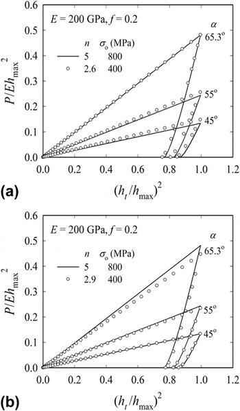
As stated above, Chen et al. ^{Reference Chen, Ogasawara, Zhao and Chiba5} and Lee et al. ^{Reference Lee, Lee and Kim6} demonstrated that different materials may have equal load–depth curves and thus equal Kick's law coefficients C. Therefore, a unique stress–strain curve cannot be obtained from a single P–h _t curve. In this study, we calculate C values by regressing the data for (0.5–1) × h _max as Lee et al. ^{Reference Lee, Lee and Kim6} suggested. Figure 9 shows the load–depth curves of two different materials (case I: σ₀ = 800 MPa, n = 5; σ₀ = 400 MPa, n = 2.6; case II: σ₀ = 800 MPa, n = 5; σ₀ = 400 MPa, n = 2.9) with equal C and E for α = 65.3°, 55°, and 45°. While for some α, the load–depth curves coincide, they do not for other α (Fig. 9). Table II lists the gaps between C values of two materials for three α. For instance in case I, the difference between C values increases from 0 to 11% when α changes from 65.3° to 45°. This means, such two materials can be distinguished by using two self-similar indenters with different centerline-to-face angles.

FIG. 9.

Load versus depth curves for different material properties with the same C and E for (a) α = 65.3° and (b) α = 45°.

TABLE II.

Comparison of C values with three centerline-to-face angles.

V. NUMERICAL APPROACH BASED ON FEA SOLUTION

A. Dual indentation method for triangular pyramidal indenter

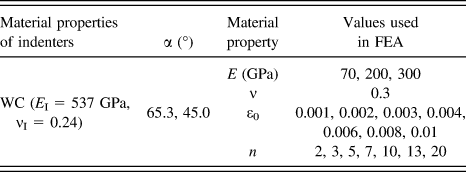
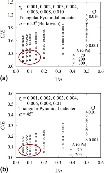
Based on the FE analysis results for a total of 294 cases (E: 3 × ε₀: 7 × n: 7 × α: 2, Table III), we propose a method for determining material properties using two triangular pyramidal indenters. In Fig. 10, C/E versus 1/n curves are shown for various values of ε₀ and α = 65.3° and 45°. The C values normalized by E are regressed to the following function

(10) $$\eqalign{ &#x0026; {{{C_i}} \mathord{\left/ {\vphantom {{{C_i}} E}} \right. \kern-\nulldelimiterspace} E} = \mathop {{f_i}}\nolimits^{{\rm{TP}}} \left( {{\varepsilon _0},n} \right) = \mathop {{f_i}}\nolimits^{{\rm{TP}}} \left( {{\varepsilon _0}} \right){n^{ - j}} = \left( {{\psi _{ijk}}\mathop {{\varepsilon _0}}\nolimits^k } \right){n^{ - j}} \cr &#x0026; \quad\!\quad i = 1,2{\rm{\ }};\quad j,k = 0,1,2,3\quad {\rm{.}} \cr}$$

TABLE III.

Material properties for FE analyses.

FIG. 10.

C/E versus 1/n curves for various values of yield strain for (a) α = 65.3° and (b) α = 45°.

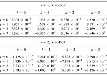
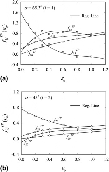
The indices i = 1 and 2 correspond to α = 65.3° and 45°, respectively. The fitting coefficients ψ _ijk are given in Table IV. Regression curves are plotted in Fig. 11. Equation (10) is the regression equation for the material with E = 200 GPa.

TABLE IV.

Coefficients ψ _ijk of Eq. (10).

FIG. 11.

Regression curves of f _ij ^TP(ε₀) in Eq. (9) versus ε₀ (third regression) for (a) α = 65.3° and (b) α = 45°.

Based on additional analysis results for E = 70, 200, 300 GPa and inserting Eq. (9) into Eq. (10) we can write

(11) $$\!&#x0026; {C_1} = E\mathop {{f_1}}\nolimits^{{\rm{TP}}} \left( {{\varepsilon _0},n} \right) = {{\mathop {{f_1}}\nolimits^{{\rm{TP}}} \left( {{\varepsilon _0},n} \right)} \over {M{f^{{\rm{TP}}}}\left( {{\varepsilon _0},n} \right) - N}} \leftrightarrow F\left( {{\varepsilon _0},n} \right) \quad\quad\quad\quad\quad\quad\quad\;\;\equiv {{\mathop {{f_1}}\nolimits^{{\rm{TP}}} \left( {{\varepsilon _0},n} \right)} \over {M{f^{{\rm{TP}}}}\left( {{\varepsilon _0},n} \right) - N}} - {C_1} = 0 \cr &#x0026; {C_2} = E\mathop {{f_2}}\nolimits^{{\rm{TP}}} \left( {{\varepsilon _0},n} \right) = {{\mathop {{f_2}}\nolimits^{{\rm{TP}}} \left( {{\varepsilon _0},n} \right)} \over {M{f^{{\rm{TP}}}}\left( {{\varepsilon _0},n} \right) - N}} \leftrightarrow G\left( {{\varepsilon _0},n} \right) \quad\quad\quad\quad\quad\quad\quad\quad\!\!\!\equiv {{\mathop {{f_2}}\nolimits^{{\rm{TP}}} \left( {{\varepsilon _0},n} \right)} \over {M{f^{{\rm{TP}}}}\left( {{\varepsilon _0},n} \right) - N}} - {C_2} = 0 \cr &#x0026; M = {{2\beta \sqrt {{A_{\rm{t}}}} } \over {S\left( {1 - {\nu ^2}} \right)\sqrt \pi }},\quad N = {{\left( {1 - \mathop {{\nu _{\rm{I}}}}\nolimits^2 } \right)} \over {E\left( {1 - {\nu ^2}} \right)}}\quad {\rm{.}} \cr}$$

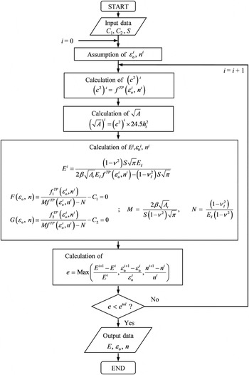
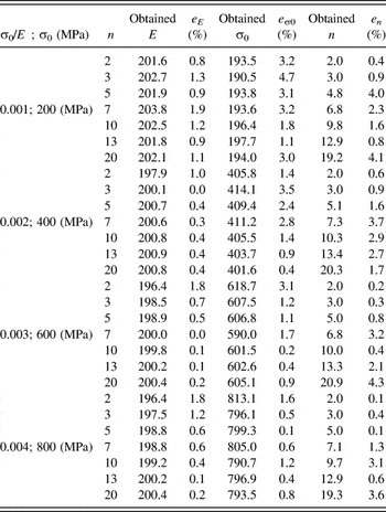
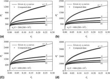
Values of ε₀ and n are determined so that F = 0 and G = 0 are satisfied. Based on Eq. (11), a program is established that extracts material properties from load–depth input data from indentations using two triangular pyramidal indenters with different α values (Fig. 12). First, C ₁, C ₂, and S are obtained from the P–h _t curves. Second, we assume initial values for ε₀ and n. c ² is then calculated from Eq. (8). E is computed from Eq. (9) based on c ² and S. We then update ε₀ and n until F = 0 and G = 0 in Eq. (11) are satisfied. E, ε₀, and n values obtained with the program are provided in Table V; the corresponding stress–strain curves are shown in Fig. 13. The average error from FE input values is about 2% for the whole range of material properties.

FIG. 12.

Flow chart for determination of material properties.

TABLE V.

Comparison of obtained material property values to those given for E = 200 GPa.

FIG. 13.

Comparison of computed stress–strain curves to those given for E = 200 GPa using WC indenter [ε₀ = (a) 0.001, (b) 0.002, (c) 0.003, and (d) 0.004].

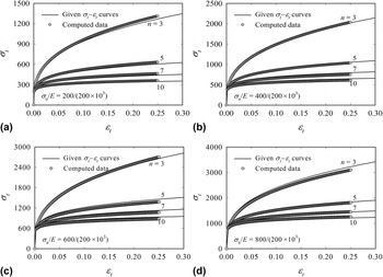
The program established with WC indenters (E _I = 537 GPa, ν_I = 0.24) is also applicable for other elastic moduli, since the key variable is ε₀ (and not E or σ₀) as noted above. Inputting P–h _t data obtained with a diamond indenter (E _I = 1000 GPa, ν_I = 0.07) into the program, and replacing the properties of WC indenter with those of diamond indenter in Eqs. (9) and (11), we obtain material properties, which are very close to those from the WC indenter (Fig. 14). The studies of Lee et al. ^{Reference Lee, Kim and Lee11,Reference Beghini, Bertini and Fontanari12} and Hyun et al. ^{Reference Hyun, Kim, Lee and Lee21} provided a similar outcome.

FIG. 14.

Comparison of computed stress–strain curves to those given for E = 200 GPa using diamond indenter [ε₀ = (a) 0.001, (b) 0.002, (c) 0.003, and (d) 0.004].

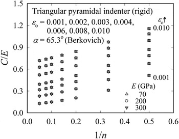
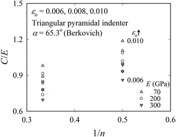
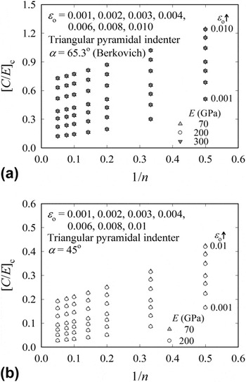
In contrast to rigid indenters (Fig. 15), C/E obtained with elastic indenters shows some sensitivity to E (Fig. 16). Owing to the indenter deformation, C/E values become sensitive to E for ε₀ > 0.005 and n < 3. However, in engineering practice, ε₀ and n are generally <0.005 and >3, respectively (circled region of Fig. 10), so that the program based on C/E can be regarded as valid for engineering purposes. Since the values of C/E are not equal for some material property combinations, we account for the indenter deformation by introducing a correction to make the approach independent of indenter deformation. C/E and P _max for rigid indentation are higher than the corresponding values obtained with an elastic indenter. The approach is discussed in detail in a previous study of ours. ^{Reference Kim, Bang, Rickhey and Lee33} Figure 17 demonstrates that the correction yields equal C/E values independent from E.

FIG. 15.

C/E versus 1/n curves from rigid indenter for various values of yield strain.

FIG. 16.

Enlargement of Fig. 10(a) for the region of ε₀ > 0.005 and n < 3.

FIG. 17.

[C/E] _c versus 1/n curves for various values of yield strain for (a) α = 65.3° and (b) α = 45°.

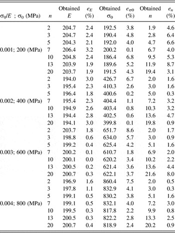
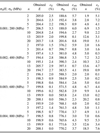
We check the sensitivity of our approach to a change in C. We assumed an error of 2%, which is equal to the error reported by Chollacoop et al. ^{Reference Chollacoop, Dao and Suresh8} for real indentation experiments. C ₁ and C ₂ are simultaneously increased (or decreased) equally by 2%. The error in the estimated properties is about 3% on average (Tables VI and VII). We may therefore state that the proposed method has a rather weak sensitivity to an error in input parameters C ₁ and C ₂.

TABLE VI.

Comparison of obtained property values (E = 200 GPa, C ₁: 2% ↑, C ₂: 2% ↑).

TABLE VII.

Comparison of obtained property values (E = 200 GPa, C ₁: 2% ↓, C ₂: 2% ↓).

B. Evaluation of material properties from experimentally obtained stress–strain curves

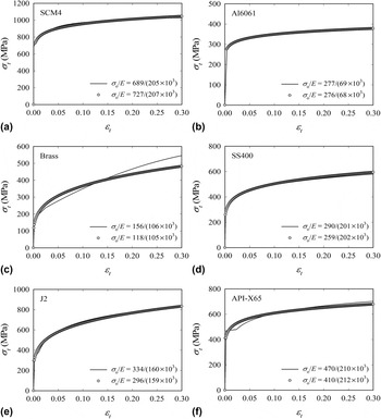
Indentation test simulation is conducted by using the tension/compression stress–strain curve data of six actual materials from the MTS hydraulic universal material tester. Figure 18 compares the stress–strain curve from the program with the actual values. The solid line refers to the tension/compression test and the gray line is the result from the program. The predicted stress–strain curves agree well with the given stress–strain curve except for brass. For brass, yield strength from the dual indentation method is 118 MPa, far from the actual yield strength (156 MPa). In the materials disobeying the power law, the difference between the actual and estimated σ₀ is large. To estimate the properties for the materials like brass, regression functions with more variables should be used.

FIG. 18.

Comparison between stress–strain curves computed by two parameter regression of the total strain range and those measured by experiment for (a) SCM4, (b) Al6061, (c) Brass, (d) SS400, (e) J2, and (f) API-X65.

VI. SUMMARY

Triangular pyramidal indentation has different characteristics compared to conical indentation. It is noteworthy that nonequal projected contact areas of two indenters and nonplanar contact line of Berkovich indenter are the main sources of different indentation characteristics of two indenters. We observed that two materials having the same C for a given indentation angle can be distinguished by using indenters with different indenter angles. Based on dual triangular pyramidal indentations, mapping functions were established to convert indentation load–depth to E, ε₀, and n. The proposed method holds for a wide range of material properties, with an average error <2%, and shows low sensitivity to errors in the input values of C ₁ and C ₂.