

1. Introduction
On 4 November 2016, the legally-binding Paris Agreement entered into force. To date, 192 signatory Parties have ratified the Agreement,Footnote 1 which aims to limit global warming to well below 2°C compared to pre-industrial levels, and to achieve a climate neutral world by mid-century. Of these, 130 countries have set a formal target or are considering a target of reducing greenhouse gas (GHG) emissions to ‘net zero’ by 2050.
Carbon taxes are likely to play a key role in curbing carbon emissions to a level that is consistent with these commitments. In this article, we assess the macroeconomic effects of a carbon tax on the global economy, paying particular attention to the terms-of-trade implications for importers and exporters of fossil fuels. The emphasis of this study is on the carbon tax as a policy instrument. This differs from climate scenarios developed, for example, by the Network for Greening the Financial System (NGFS, 2019),Footnote 2 where the emphasis is on developing a common reference framework for central banks and supervisors of long-term temperature pathways, the energy composition and climate policy intensity consistent with those pathways, and the interactions between the physical risks from climate change and the economic risks associated with different transition pathways. The focus of this study is, rather, on isolating the macroeconomic transmission channels of a carbon tax. A key contribution of this article is that by isolating the carbon tax channel we are able to decompose the impacts on potential output into the shares driven by the long-run terms-of-trade shock and the shares driven by the impact of the tax on factor inputs.
We use a modified version of the National Institute’s Global Econometric Model, NiGEM, to explore the impact of a carbon tax under different fiscal policy reaction functions. NiGEM is a peer reviewed global macroeconomic model that has developed over 30 years of regular use, and is widely used by central banks, finance ministries and other public and private bodies around the world for forecasting, scenario analysis and stress testing. NiGEM’s Climate Model was initiated in 2018, to model the interactions between the macroeconomy and climate-related shocks and climate-related policy instruments. The Climate Model integrates key policy channels, such as a carbon tax and border carbon adjustments, into the well-established macroeconomic framework of NiGEM. The global model allows users to model policy developments in a single country, in a group of countries, or at the global level, and to assess the economic spillovers between countries via trade and financial markets. For the purpose of this article, we modify the production function underlying NiGEM to fully capture the long-run impacts of a large, permanent terms-of-trade shock.
This study develops a set of stylized scenarios where all countries and regions impose a permanent and uniform carbon tax immediately. The simulations show that demand for fossil fuels falls substantially in response to the tax, global (pre-tax) prices of fossil fuels decline, and the tax has the potential to raise substantial revenue for the government. A $50 global carbon price, with offsetting cuts in income taxes, would be expected to raise consumer prices at the global level by about 2.5 per cent, reduce world output by about 0.8 per cent, and reduce global carbon emissions by about 11 per cent. Given the relatively small magnitude of the shock considered here, this study abstracts from any of the positive physical impacts that slowing the pace of climate change may have on productive capacity. The overall impact on GDP growth and inflation in each country depends on the fossil fuel intensity of output, the net losses/gains in terms of trade and the macroeconomic policy reaction. Economies where the production structure is heavily dependent on fossil fuels are heavily exposed. At the same time, fossil fuel exporting countries that rely on the export revenue from fossil fuel sales are also heavily impacted by the shock. On the other hand, the impact on many countries in Europe may be relatively small in response to a low-carbon tax, because the region relies less on fossil fuel and especially coal, which creates a higher level of carbon emissions compared to oil and gas.
The fiscal policy reaction has important implications for scenario results (see also McKibbin et al., Reference McKibbin, Morris, Wilcoxen and Liu2018). The impact on GDP, in both the short and longer term, is expected to be smallest when the government channels revenue from the carbon tax directly into productive investment. However, many forms of policy design may generate little or no fiscal revenue, limiting the scope for fiscal policy to smooth the adjustment required to transition to a low-carbon economy.
2. The role of carbon taxes
Human activity has played a central role in generating the greenhouse gases that are responsible for global warming and climate change. According to the Intergovernmental Panel on Climate Change ‘It is unequivocal that human influence has warmed the atmosphere, ocean and land. Widespread and rapid changes in the atmosphere, ocean, cryosphere and biosphere have occurred’ (IPCC, Reference Masson-Delmotte, Zhai, Pirani, Connors, Péan, Berger, Caud, Chen, Goldfarb, Gomis, Huang, Leitzell, Lonnoy, Matthews, Maycock, Waterfield, Yelekçi, Yu and Zhou2021). This has already affected weather and climate extremes across the world, including heatwaves, heavy precipitation, droughts and tropical cyclones. Studies by the World Weather AttributionFootnote 3 and the BAMS special reportFootnote 4 assess the role of human-caused climate change in specific extreme weather events, and how the frequency and intensity of such events can be expected to change as global temperatures increase.
GHG emissions are set to continue rising without stringent policy intervention, with mean projected warming expected to be in the range of 2.6–7°C above pre-industrial levels by 2100. Temperatures above 2° warming will lead to more intense and frequent weather events such flooding, droughts, tropical cyclones and fire weather, as well as cause further damage to the ecosystem and rising sea levels (IPCC, Reference Masson-Delmotte, Zhai, Pirani, Connors, Péan, Berger, Caud, Chen, Goldfarb, Gomis, Huang, Leitzell, Lonnoy, Matthews, Maycock, Waterfield, Yelekçi, Yu and Zhou2021). There is broad consensus that market forces alone will not be sufficient to restrict GHG emissions to levels consistent with the Paris Agreement. GHG emissions are a textbook example of a negative externality. Emissions carry a very heavy cost that is borne by society, as we all suffer from the impacts of climate change, pollution associated with burning fossil fuels, and the risks to our planet. These social costs of emissions are far greater than the private costs incurred by the emitter, and so are not fully reflected in their cost-benefit analysis when evaluating production and consumption choices. This market failure is complicated by two additional factors. First, the most serious costs of climate change are expected to take place beyond a typical election cycle, whereas the cost of adjustment is immediate. Second, there is a likely mismatch between those that bear the brunt of the costs of climate change and climate change mitigation policies and those that are responsible for the lion’s share of GHG emissions, both past and present.
Stern and Stiglitz (Reference Stern and Stiglitz2021) propose two ways of calculating the social cost of carbon: (a) to look at the future damage from emitting an extra unit of carbon and (b) to look at the carbon prices that could guide the behavioural changes towards emission reduction pathways that will limit the rise in global temperature to 1.5–2°.
Carbon policy interventions aim to transfer some of the social costs of emissions to the emitters, and to encourage households, firms and governments to invest, adopt and instil practices that limit or even help reverse the damage caused by carbon intensive activities. These interventions may be implemented via fiscal instruments, such as a carbon taxes and tax incentives, or subsidies for corporations and households that are designed to encourage transition to a low-carbon economy. For example, a carbon tax raises the costs of high-emitting activities relative to low-emitting activities, which in turn impacts our choices of production technologies to use and our choices of goods and services to buy. Regulatory interventions, such as cap-and-trade systems that impose a quantitative limit on emissions, can deliver similar outcomes. There are also policies that help address other market failures related to capital markets, R&D and innovation, information and networks and co-benefits (Stern and Stiglitz, Reference Stern and Stiglitz2021) and some of these interventions have gained prominence recently. Good examples from the financial sector are the initiatives taken by central banks to facilitate appropriate asset price valuations that fully account for a firm’s carbon footprint; macroprudential measures that aim to establish a clear understanding of climate-related financial stability risks; and proposals to adjust central bank portfolios and collateral frameworks to favour low-carbon assets (Krogstrup and Oman, Reference Krogstrup and Oman2019; NGFS, 2019).
In this article, we focus on an explicit carbon tax. Pricing carbon dioxide (CO2), which constitutes about three-quarters of global GHG emissions, is widely thought to form an important part of any energy transition strategy, and in some cases may be the most cost-effective way to reduce GHG emissions (OECD, 2016). The tax will raise the price of burning fossil fuels in proportion to the amount of carbon that is emitted by each fuel. This delivers a shift in the relative prices of energy sources. For example, the price of burning carbon-heavy coal will rise significantly relative to carbon-free renewable energy sources. By internalising some of the social costs of carbon, the tax encourages transition to more carbon-efficient energy sources and the tax also incentivises firms to innovate in more clean technologies (Aghion et al., Reference Aghion, Dechezleprêtre, Hémous, Martin and Van Reenen2016). The explicit carbon tax modelled here can also be interpreted as a proxy for the intensity of environmental policy. For example, regulation can have a similar effect, requiring firms to invest in more carbon-efficient production technologies, and can be thought of as a shadow carbon price. An explicit tax, however, also has the potential to raise significant government revenues, at least during a transition phase (for the United States see Congressional Budget Office, 2011).
A unilateral carbon tax imposed by a single country may lead to a loss in competitiveness and a relocation of carbon intensive activities to countries with more lax emission policies, with minimal overall impact on global carbon emission (McKibbin et al., Reference McKibbin, Morris, Wilcoxen and Liu2018). This is known as carbon or emissions leakage. The obvious response to this is a border carbon adjustment where the country imposing the carbon tax introduces an import tax for goods and services from countries with less-stringent emissions standards and alongside that a tax rebate for exporting companies to re-establish a level-playing field. The European Union’s Carbon Border Adjustment Mechanism (CBAM), currently under discussion, is a prime example.Footnote 5 In this article, we abstract from these issues, which have not been resolved at the level of the World Trade Organization, by running a set of illustrative scenarios where all countries and regions impose a common carbon tax.
Our analysis is stylised in other important ways. Imposition of a carbon tax of this size is likely to drive technological advances that will lead to improved energy efficiency. The speed of adoption of these new technologies will vary across different economies, and we have made no explicit assumption on the rise in energy efficiency. These taxes could also lead to stranded assets as some high-emitting economic activities will simply no longer be viable (Jaffe, Reference Jaffe2020). While stranded assets are not explicitly modelled in this article, a carbon price that increases the user cost of capital has a similar impact on investment as a rise in the rate of depreciation associated with asset stranding.
This study sheds light on country-specific differences that arise from the structure of the economy and the choices made by households, firms and policy makers. For example, countries that have a higher energy intensity of output and those that consume carbon intensive fuels such as coal are more vulnerable compared with countries that predominantly use gas or renewables. Economies that rely on fossil fuel exports (especially oil and coal) also stand to lose. By applying a uniform carbon tax across the world, we also show that spillovers matter, amplifying the global economic costs of a carbon tax. The overall impact on GDP, potential output, inflation, and other key macroeconomic variables will also depend on the response of the fiscal and monetary authorities. We discuss the role of these channels in this article.
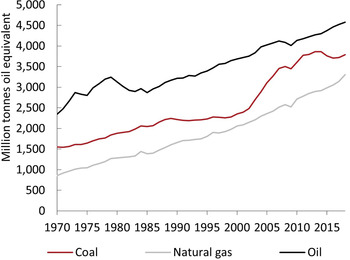
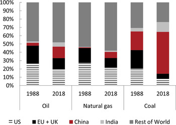
Figure 1 shows the global consumption of three fossil fuels—gas, coal and oil—over time. Oil remains the most important fuel, followed by coal and gas. Over this period coal has gained importance mainly because of rapid growth in demand in China and India. China’s share of world coal consumption rose from 20 per cent in 1998 to 50 per cent in 2018. India’s share of world coal consumption has also risen over this period from 4 per cent to 11 per cent (figure 2). The economies of China and India are therefore more exposed to a carbon tax than Europe and the US, where coal consumption has generally declined over the last two decades, with rising shares of more carbon-efficient fuels such as gas and renewables.
(Colour online) World consumption of fossil fuels.
Source: NiGEM database.

(Colour online) Share of global fossil fuel consumption by major countries/regions.
Source: NiGEM database.

Our simulations assume that the tax burden is borne by firms in the first instance. In response, a profit maximising firm could pass on the additional cost to households through higher prices, adjust the wage bill or adjust capital spending.
The government, in turn, can recycle the tax revenue to households through the taxation system, use it to invest in an expansion of renewable energy supply, surgically target the more vulnerable sections of society through transfers, or reduce corporation taxes and provide incentives to encourage private sector investment in green technologies. The negative impact on economic growth will be particularly large if instead the tax revenue is used to pay down government debt, unless that leads to a significant reduction in the sovereign risk premium.
The overall macroeconomic impact will also depend on the behavioural and monetary policy response. Will consumer preferences change in response, and will the new tax have any lasting impact on inflation expectations? From a monetary policy point of view, a carbon tax has supply shock features with output expected to fall and prices expected to rise. Will the central bank accommodate the shock in the belief that inflation expectation will remain anchored?
3. Interactions between energy transition and terms of trade
A country’s terms of trade are determined by the revenue potential of the country’s exports compared to the costs of importing desired goods and services from abroad. Export revenue depends on both the volume of goods and services that are exported and the value of those goods and services in domestic currency. Terms of trade, therefore, depend on three factors: the relative volumes of exports and imports; the relative prices of exports and imports; and the exchange rate.
Measures such as real gross domestic income capture gains and losses in the terms of trade, whereas headline GDP does not. The relationship between the two can be approximated by deflating exports and imports by the price of domestic demand, rather than their respective trade deflators:
 $$ \mathrm{GDI}\hskip1.5pt =\hskip1.5pt \mathrm{DD}+\frac{\mathrm{XV}}{{\mathrm{P}}^{\mathrm{DD}}}-\frac{\mathrm{MV}}{{\mathrm{P}}^{\mathrm{DD}}}, $$
 $$ \mathrm{GDP}\hskip1.5pt =\hskip1.5pt \mathrm{DD}+\frac{\mathrm{X}\mathrm{V}}{{\mathrm{P}}^{\mathrm{X}}}-\frac{\mathrm{M}\mathrm{V}}{{\mathrm{P}}^{\mathrm{M}}}, $$
where GDI, gross domestic income, constant prices; GDP, GDP, constant prices; DD, domestic demand, constant prices; XV, exports, current prices; MV, imports, current prices; PDD, deflator for domestic demand; PX, deflator for exports (domestic currency); PM, deflator for imports (domestic currency).
As the world progresses towards environmental targets, including a low-carbon production structure, demand for carbon-heavy fuels such as coal and oil can be expected to decline. This decline in demand can also be expected to put downward pressure on the (pre-tax) price of fossil fuels. Countries that continue to rely heavily on fossil fuel exports can be expected to suffer a significant loss in potential export revenue, stemming from both a decline in the volume of demand for fossil fuels and a decline in the value of each tonne of fossil fuel that continues to be exported. This will deliver significant terms-of-trade losses for fossil fuel exporters, via the channel described by XV in equation (1). This, in turn, will act as a constraint on GDP, as income losses feed into lower levels of domestic demand.
Meanwhile, many fossil fuel importers may experience gains in terms of trade, as they transition towards a production structure that includes a greater share of domestically produced energy from renewable sources. This will materialise via the channel MV in equation (1).
The magnitude of terms-of-trade shocks experienced in each country will depend on factors such as the share of domestic income derived from fossil fuel exports, the flexibility of the exchange rate regime, and the capacity for and speed of structural transition in the economy towards low-carbon industry and domestically produced renewable energy sources.
4. Modelling a global carbon tax in NiGEM
We model the impact of carbon taxes using a modified version of the National Institute Global Econometric Model, NiGEM. The modified version includes NiGEM’s Climate Model and a modified production function to isolate the terms-of-trade channel. NiGEM is a peer reviewed global econometric model that has developed over 30 years of regular use. The model is used by policy makers and private sector organisations around the world for economic forecasting, scenario analysis and stress testing.
NiGEM is a Global model that consists of individual country and regional models, which are linked together through trade in goods and services and integrated capital markets. It represents a closed world, where outflows from one country or region are matched by inflows into other countries and regions. NiGEM is an Econometric model, in that key behavioural equations are econometrically estimated using historical data. This ensures that the dynamics and key elasticities of the model fit the main characteristics of individual country data. From a theoretical perspective, NiGEM can be classed among global general equilibrium macroeconomic models. It therefore strikes a balance between theoretical underpinnings that guide economies towards long-run market clearing equilibria, and data-driven individual country dynamics and elasticities that fit the main characteristics of real-world data outturns.
Based on a broadly New Keynesian structure with many of the characteristics of dynamic stochastic general equilibrium (DSGE) models, individual country models are grounded in textbook macroeconomic foundations, with features such as sticky prices, rational or model-consistent expectations, endogenous monetary policy based on a Taylor rule or other standard specifications, and long-run fiscal solvency. Country models are built around the national income identity, and contain the determinants of domestic demand, trade volumes, prices, current accounts and asset holdings. The long run is anchored by supply inputs and the long run equilibrium is achieved through price and wage adjustments. The supply inputs include labour, capital and energy. Energy is disaggregated into coal, oil, gas and non-fossil fuels (mostly renewables). NiGEM incorporates endogenous monetary and fiscal policy responses that act to stabilise output and inflation in the long run. For a full description of the standard model, see Hantzche et al. (Reference Hantzsche, Lopresto and Young2018).
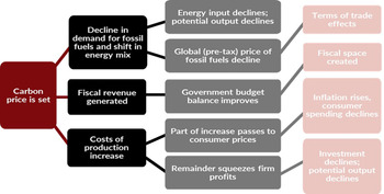
The NiGEM climate model is an expanded version of the standard model that introduces channels to model climate policy instruments, energy transition and physical climate shocks. The key channels relevant for a carbon price are detailed in the Annex. Figure 3 provides an overview of the supply and demand channels that have been introduced into NiGEM to capture the impact of carbon taxes.
NiGEM channels to allow for carbon taxes.

A carbon tax has features of a supply shock in that it raises the cost of production, while the inflationary impacts reduce demand. The tax revenue that is collected by the government can then be used to reduce debt, spent on investment, or recycled back to households and firms through taxes, subsidies or transfers.
We assume that the carbon tax is applied upstream as a rise in production costs. The majority of CO2 emissions stem from burning fossil fuels. A carbon tax has a direct impact on the cost of burning fossil fuels in proportion to the carbon that is emitted by each fuel. The rise in production costs reduces the aggregate demand for fossil fuels, and also encourages a shift in the energy mix—away from coal, and towards lower-carbon emitting fossil fuels and renewables. As aggregate demand for fossil fuels declines, this puts downward pressure on the global pre-tax price of fossil fuels. The impact of the decline in the global price depends on whether the country is a net importer or exporter of fossil fuels, with significant terms-of-trade losses for fossil fuel exporters, whereas fossil fuel importers benefit from the lower import price.
The carbon tax will raise revenue for the government, although terms-of-trade losses may constrain government spending. Country-level CO2 emissions depend on the quantities of coal, oil and gas consumed, with each fossil fuel modified by the appropriate emission factor. The level of CO2 emissions then interacts with the carbon price to derive the fiscal revenue that is generated. Higher revenue creates fiscal space that the government can then use if a variety of ways, as explored in the scenarios.
Higher production costs lower corporate profitability in the first instance. Batten et al. (Reference Batten, Sowerbutts, Tanaka, Walker, Gramlich, Bitar and Fardnia2020) cite a number of recent studies that suggest a high-level of pass-through of emission prices to electricity prices. NiGEM applies a country-specific pass-through of the carbon tax to consumer price inflation, which is based on the average historical pass-through of other indirect taxes to consumer prices. In most countries, roughly 50 per cent of the indirect tax is passed on to consumers through higher prices of non-fuel goods and services, while the remainder acts as a squeeze on firm profit margins, constraining investment. Broadly speaking, a higher transitory pass-through to inflation would imply a smaller negative impact on GDP. This stems from both the short-run volatility of investment relative to consumption, and the long-run impact of foregone investment on productive capacity.
Equation (3) illustrates the underlying production function in NiGEM.
 $$ \mathrm{YCAP}\hskip1.5pt =\hskip1.5pt \gamma {\left\{{\left[s{(K)}^{-\rho }+\left(1-s\right){\left(L{e}^{\lambda t}\right)}^{-\rho}\right]}^{-1/\rho}\right\}}^{1-\alpha }{M}^{\alpha }, $$
where YCAP, potential output; γ, scaling factor, which we treat as a function of terms of trade
 $ \left(\gamma \hskip1.5pt =\hskip1.5pt {\gamma}_1\frac{\overset{\sim }{P^X}}{\overset{\sim }{P^M}}\right) $
;
 $ \overset{\sim }{P^X,} $
trend deflator for exports (domestic currency)—4 quarter moving average;
 $ \overset{\sim }{P^M,} $
Trend deflator for imports (domestic currency)—4 quarter moving average; K, productive capital stock; L, potential labour input; λt, labour augmenting technical progress; M, effective energy input, adjusted for energy efficiency gains; α, the energy share of production costs; ρ, a parameter related to the elasticity of substitution between capital and labour (
 $ \sigma \hskip1.5pt =\hskip1.5pt \frac{1}{1+\rho } $
); s, scaling factor.
The transmission of a carbon price to potential output on the supply side enters via three channels:
-
• The constraint on total energy input into production (M) in response to the rise in energy prices. This may be partially offset by efficiency gains, but for the purpose of these scenarios we hold energy efficiency constant.
-
• The decline in the accumulation of capital stock (K) in response to the profit squeeze faced by firms, which reduces the return on investment (or raises the user cost of capital).
-
• Any permanent shift in terms of trade, which enters via γ. We isolate the impact of this channel by running the scenario with γ exogenous (no terms-of-trade effects) and with γ endogenous (terms-of-trade channel activated).
To the extent that a carbon tax reduces global carbon emissions and slows the pace of climate change, the negative impacts of a carbon tax on potential output may be partially offset by positive impacts related to physical climate shocks. For example, fewer and less intense storms would slow the rate of capital depreciation and more stable temperatures could increase labour productivity. These channels are not considered in this article.
5. Carbon tax scenarios and simulation results
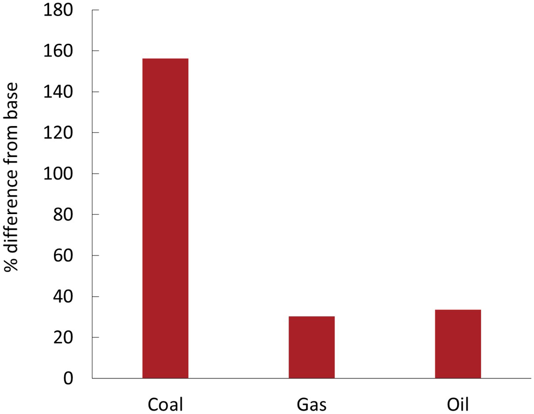
To explore the potential impacts of a carbon price, we run, as a diagnostic example, a series of scenarios that introduce a carbon tax of $50 per tonne of CO2 emitted. This is in line with the social cost of carbon estimated by the Interagency Working Group in the Obama Administration, but considerably lower than more recent estimates of the social cost of carbon associated with Net Zero targets (Stern and Stiglitz, Reference Stern and Stiglitz2021). The tax is permanent and is applied uniformly across all regions and countries immediately. The carbon tax is imposed on each fossil fuel (coal, gas and oil) in proportion to the CO2 that is emitted when burning the fuel and scaled by the energy that is produced by each fuel (BP, 2019; Vermeulen et al., Reference Vermeulen, Schets, Lohuis, Kolbl, Jansen and Heeringa2018). This drives a post-tax shift in the relative price of different energy inputs. Fossil fuel prices rise significantly relative to renewables, as illustrated in figure 4. The results are presented against a baseline scenario under which no new climate policy is introduced.
(Colour online) Impact of $50 carbon tax on post-tax fossil fuel prices relative to renewables.
Source: NIGEM simulation.

A $50 carbon price would more than double the post-tax price of coal relative to renewable energy. The prices of gas and oil would rise relative to renewables by 30–35 per cent, with the price of oil up by roughly $20–25 per barrel.
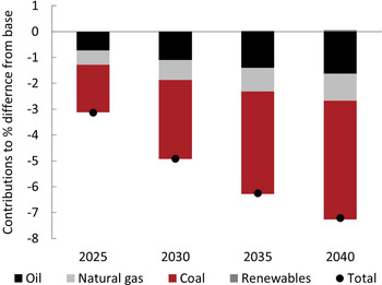
The rise in the cost of energy drives a decline in aggregate energy demand, while the shift in relative prices delivers a gradual shift in the composition of energy demand, away from coal in particular. Figure 5 illustrates the expected impact on total global energy demand by fuel type over the next 20 years. Total energy demand would be expected to decline by roughly 7 per cent, with coal delivering more than half of the decline. This is expected to push global carbon emissions down by about 11 per cent.
(Colour online) Impact of $50 carbon tax on global energy demand.
Source: NIGEM simulation.

The decline in energy demand enters the production function via M in equation (3), leading to a decline in potential output. The energy intensity of production will also decline, as α is less than 1. But we have introduced no explicit assumption on how a carbon price might also encourage investment in energy efficiency gains or renewable energy research, both of which have the potential to partially offset the modelled decline in effective energy input illustrated in figure 5.
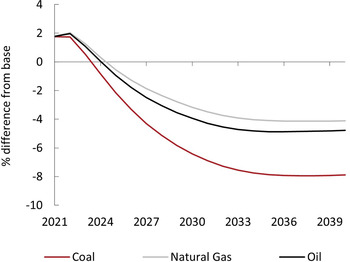
The decline in energy demand puts downward pressure on pre-tax global fossil fuel prices, which slightly offsets the post-tax price rise. Figure 6 illustrates the expected decline in pre-tax global prices. The global price of coal drops by about twice the decline in the price of gas. This would reduce the profitability of producing coal and other fossil fuels for export, accelerating the shift away from coal use. In the short-term, nominal fossil fuel prices are expected to rise by about 2 per cent, in response to the rise in global inflation and different speeds of adjustment of supply and demand in energy markets.
(Colour online) Impact of $50 carbon tax on world price of oil, gas and coal.
Source: NIGEM simulation.

To assess the potential impact of the shock on GDP we consider two sets of scenarios. First, we isolate the impact of the terms-of-trade channel on potential output. We first run the scenario treating γ (equation (3)) as exogenous, so that there are no permanent terms-of-trade effects on potential output. We run the same scenario a second time, with the terms-of-trade channel activated via γ.
Second, we run a set of scenarios with endogenous terms-of-trade effects, but look at different fiscal policy reaction functions to illustrate the importance of the policy response to the final scenario output. In all scenarios, monetary policy is endogenous and follows the default 2-pillar rule in NiGEM, which means that interest rates respond to shifts in inflation and nominal GDP growth.
5.1. Isolate terms-of-trade effects
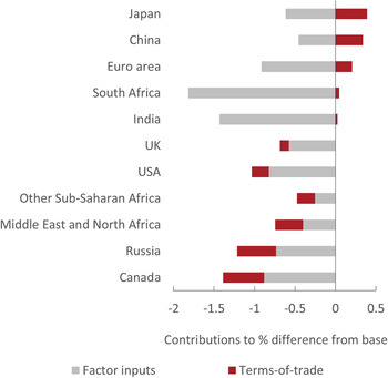
Figure 7 disaggregates the transmission to potential output of the $50 carbon tax into impacts driven by adjustments in factor inputs (energy and capital) and those driven by the terms-of-trade shock. The impacts of terms of trade are positive in countries such as Japan, China and the Euro Area, which are heavily reliant on imports of fossil fuels. Fossil fuel exporters, such as Canada, Russia and the Middle East, on the other hand, see terms-of-trade losses amplifying their adjustment in factor inputs. Potential output losses in South Africa and India are expected to be particularly high, as both countries remain heavily dependent on coal.
(Colour online) Long-run impact on potential output of $50 carbon tax.
Source: NIGEM simulation. Scenario run with NiGEM’s default fiscal policy settings, with carbon revenue allowing a gradual adjustment in income taxes to maintain a stable fiscal balance.

5.2. Explore fiscal policy reaction functions
The next set of scenarios considers three potential fiscal policy responses to the shock. In all cases, terms of trade are endogenous in the production function.
-
• In Scenario 1, NiGEM’s default fiscal policy settings are applied, consistent with the results illustrated in figure 7. This applies a solvency rule to government finances, which triggers an endogenous adjustment in the income tax rate when the fiscal balance deviates from the baseline target. Carbon revenue will improve the fiscal balance, although this will be partially offset by government revenue losses associated with the decline in output, especially in countries where government finances are heavily reliant on revenue generated from fossil fuel exports. In most countries, we expect a gradual decline in the income tax rate over the simulation horizon.
-
• In Scenario 2, we consider an alternative fiscal response, where 100 per cent of the carbon revenue is channelled into government investment. This acts as a short-term stimulus to demand, and also accumulates as capital stock, raising the long-run level of potential output. Income tax rates remain endogenous and would be expected to rise in many countries to offset revenue losses elsewhere.
-
• In Scenario 3, we recall that the carbon price is indicative of the government’s environmental policy effort, which in some cases may be effected through policy measures that do not generate a government revenue stream. In this case, there is no revenue generated from the carbon price to flow onto the fiscal balance. This limits the scope for fiscal policy to accommodate the shock without allowing government debt to rise. Income tax rate are exogenous, to illustrate the magnitude of the negative carbon price shock on the fiscal position.
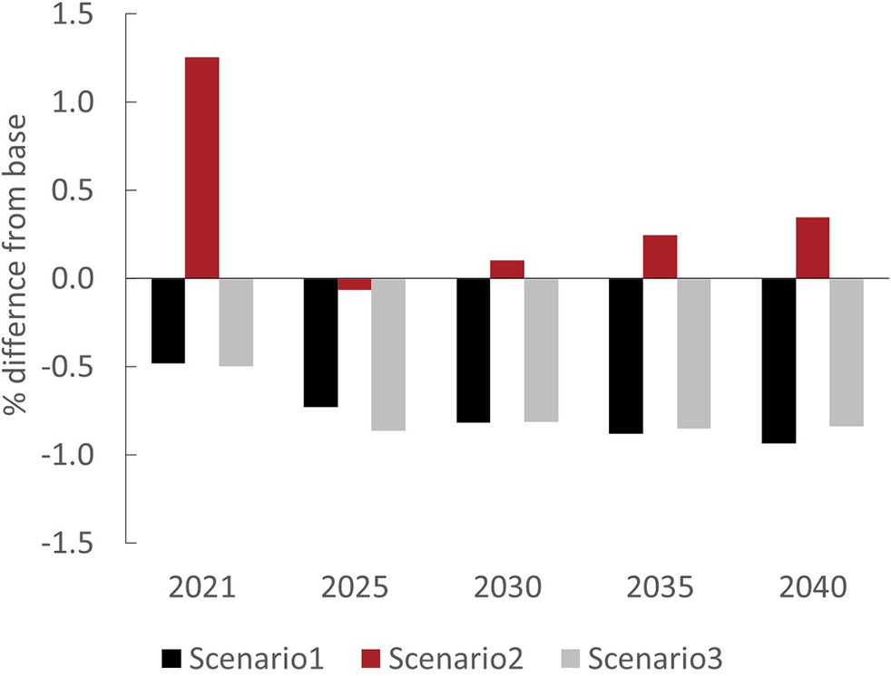
The impact on global GDP in the three scenarios is illustrated in figure 8. With no government revenue stream (Scenario 3), the negative impact of the introduction of a carbon tax on global output is amplified in the short-term. This illustrates the important role for fiscal policy to smooth the transition path in response to the shock. On the other hand, if all the potential government revenue from a carbon price is channelled into government investment (Scenario 2), global output would be expected to be at least 1 per cent higher by 2040 compared to the other two scenarios. The accumulation of capital stock over a 20-year period builds economic capacity over the course of the transition, fully offsetting the associated costs of the carbon tax, at least at the global level. Individual countries may still face a net cost from the policy, depending on the magnitude of the country-specific shocks posed by the energy transition. While we have not specified how the investment would be spent, some areas that could further accelerate the energy transition include renewable energy infrastructure, retrofitting of buildings, research to support energy efficiency gains or carbon capture technology, and so forth. In fossil fuel exporting countries, the priority may be to support the development of new low-carbon industry to compensate for the inevitable job losses in fossil fuel sectors.
(Colour online) Impact of $50 carbon tax on global GDP under different fiscal options.
Source: NIGEM simulation. Scenario 1, Gradual adjustment in income tax; Scenario 2, Carbon revenue channelled to government investment; Scenario 3, No government revenue generated.

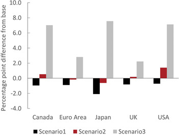
The profile of government debt also differs across the scenarios (figure 9). With a fiscal rule designed to stabilise the fiscal balance through income tax adjustments, debt would generally be expected to decline slightly if carbon revenue is generated and allowed to flow onto the fiscal balance (Scenario 1). If there is no fiscal revenue generated and income taxes are held fixed (Scenario 3) government debt would rise given the negative impact on economic activity overall. When carbon revenue is directed towards a government investment programme (Scenario 2), the net impact on government debt is more ambiguous, and will depend on other country-specific developments, including the sensitivity of inflation to the carbon tax, the monetary policy reaction and exchange rate developments.
(Colour online) Impact of $50 carbon tax on government debt (% of GDP) by 2040 under different fiscal options.
Source: NIGEM simulation. Scenario 1, Gradual adjustment in income tax; Scenario 2, Carbon revenue channelled to government investment; Scenario 3, No government revenue generated.

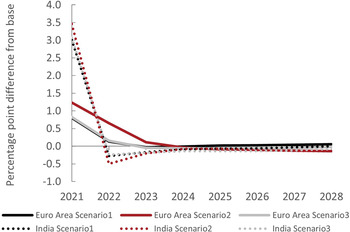
Introduction of a carbon tax temporarily drives inflation higher in all countries and regions under all three scenarios. These temporary impacts dissipate within 5 years in most countries. The short-term inflationary impacts tend to be higher under Scenario 2, when carbon revenue is channelled into government investment, as the impact of the carbon price is accompanied by the short-term stimulus from higher investment. Figure 10 illustrates the impacts on inflation in the Euro Area and in India as an example. Higher inflation in India, which is expected to rise by 3–3.5 per cent initially, reflects the higher use of coal in the economy. Recall that the post-tax price of coal is expected to rise 150 per cent in response to a $50 tax on carbon. In the Euro Area, on the other hand, inflation would be expected to rise by between 0.8 and 1.3 percentage points in the first year.
(Colour online) Impact on inflation rate of $50 carbon tax under different fiscal options in the Euro Area and India.
Source: NIGEM simulation. Scenario 1, Gradual adjustment in income tax; Scenario 2, Carbon revenue channelled to government investment; Scenario 3, No government revenue generated.

Our simulations assume that inflation expectations remain anchored, but with inflation rising to levels as high as this there is a risk that expectations may drift, especially in countries where inflation targeting is recent and central bank independence less well-established.
In addition to the short-term effects on domestic demand, the carbon tax shock is global, so that there are also indirect effects through external demand spillovers and trade prices, with a material impact on the macroeconomy.
If we were to run a separate scenario where the same $50 carbon tax is imposed unilaterally in an open economy such as the UK, inflation would be expected to rise by 0.6 percentage point less than under the global carbon tax scenario, and GDP to fall by 0.4 per cent less. This abstracts from any potential complimentary policy, such as a border carbon adjustment.
6. Conclusion
In this article, we explore the impact of a permanent and uniform $50 carbon tax applied across all economies. The oil price rises by around $25 per barrel on impact, coal prices rise by about 150 per cent and gas by 30 per cent. The shock feeds through the production function, through the rise in production costs and through import prices into the real economy. The simulations show that the carbon tax behaves like a supply side shock by exerting downward pressure on GDP and upward pressure on inflation in all economies relative to a baseline scenario. In general, countries that have a higher energy intensity of output and those that consume carbon intensive fuels are more vulnerable compared with countries that predominantly use gas or renewables. For example, India and South Africa, which continue to rely heavily on coal, are particularly exposed to the energy transition and a rising price on carbon.
The net impact on potential GDP also depends on two key factors: how the shock impacts a country’s terms of trade and how any revenue from a carbon tax is recycled into the economy. An important contribution of this article is to decompose the long-run impact from a carbon tax shock on potential output into the share attributable to terms-of-trade effects and the share attributable to direct adjustments in factor inputs (capital and energy). The impacts of terms of trade are positive in countries such as Japan, China and the Euro Area, which are heavily reliant on imports of fossil fuels. Fossil fuel exporters, such as Canada, Russia and the Middle East, on the other hand, see terms-of-trade losses amplifying the impacts of domestic adjustment.
Our results show that the fiscal policy response plays a very important role in the scenario results. When revenue from an explicit carbon tax is channelled back into the economy via government investment, this acts as a short-term stimulus to demand, and also raises potential outlook over the medium term. At the global level, this fully offsets the costs of introducing the carbon tax that stem from the rise in production costs, with potential GDP roughly 1 per cent higher by 2040 compared to the other two scenarios. A fiscal response that allows income taxes to gradually decline to offset the rise in carbon revenue will help to smooth the adjustment costs of energy transition, but would not necessarily offset the long-run losses.
There are many other fiscal policy strategies that may be considered. For example, the government can surgically target the more vulnerable sections of society through transfers or incentivise companies to invest in green technology with subsidies and adjustments to the corporation tax rules. In terms of the net impact on GDP, other fiscal policy options can be expected to fall somewhere between the extreme options presented here: 100 per cent of carbon revenue channelled to productive investment and zero carbon revenue generated. The final choice of policy design will depend on political priorities as well as the capacity to engender public support for the policy.
By applying a uniform carbon price across the world, we also show that spillovers matter. As the same tax is introduced in all countries—developed and emerging—this leads to direct impacts as well as indirect impacts from spillovers. These spillovers serve to magnify the impact of the shock. A carbon tax for the UK alone would result in inflation that is around 0.6 percentage point less than when the tax is imposed globally, while GDP would decline by around a 0.4 per cent less.
In reality, countries that rely heavily on fossil fuels may be unlikely to impose the same level of tax as those that are less reliant on fossil fuels. The scenarios presented here can be developed more deeply in the future to explore options such as border carbon adjustments by countries that have imposed a carbon tax on others that have less-stringent climate policies. A complete scenario would also include the impact of both acute and chronic physical shocks of climate change (Kahn et al., Reference Kahn, Mohaddes, Ng, Pesaran, Raissi and Yang2019) and migration. These become particularly relevant over longer horizons.
Acknowledgements
The authors would like to thank Matthew Agarwala, John Fitzerald and participants of the 17th Euroframe Conference on Economic Policy Issues in the European Union (https://www.euroframe.org/conferences.html) for helpful comments and discussion during the conference. The authors are also grateful for comments from an anonymous referee that have helped to shape the article. All errors remain our own.
A. Annex: NiGEM v3.21 climate model
For a full description of the standard NiGEM model, see Hantzsche et al. (Reference Hantzsche, Lopresto and Young2018). The NiGEM climate model is an expanded version of the standard model that introduces channels to model climate policy instruments, energy transition and physical climate shocks. The key channels relevant for a carbon price are detailed in this Annex.
A.1. Production function
The production function in NiGEM has an outer Cobb–Douglas function for energy and the capital-labour bundle. This means that in value terms, energy is modelled as a constant share of input costs, with the share given by alpha. In other words, a 1 per cent rise in energy price is offset by a 1 per cent decline in energy volume for a given level of output. The adjustment happens gradually over several years, so does not necessarily hold at any specific point in time.
 $$ \mathrm{YCAP}\hskip1.5pt =\hskip1.5pt \gamma {\left\{{\left[s{(K)}^{-\rho }+\left(1-s\right){\left(L{e}^{\lambda t}\right)}^{-\rho}\right]}^{-1/\rho}\right\}}^{1-\alpha }{M}^{\alpha }, $$
where YCAP, potential output; γ, scaling factor, which we treat as a function of terms of trade
 $ \left(\gamma \hskip1.5pt =\hskip1.5pt {\gamma}_1\frac{\overset{\sim }{P^X}}{\overset{\sim }{P^M}}\right);\overset{\sim }{P^X}, $
trend deflator for exports (domestic currency)—4 quarter moving average;
 $ \overset{\sim }{P^M}, $
trend deflator for imports (domestic currency)—4 quarter moving average; K, productive capital stock; L, potential labour input; λt, labour augmenting technical progress; M, effective energy input, adjusted for energy efficiency gains; α, the energy share of production costs; ρ, a parameter related to the elasticity of substitution between capital and labour (
 $ \sigma \hskip1.5pt =\hskip1.5pt \frac{1}{1+\rho } $
); s, scaling factor.
This 3-factor production function for full country models can be transformed into a growth rate equation if we differentiate, convert to log differentials, and use marginal product conditions that set marginal products equal to their real cost:
 $$ \frac{d log\left(\mathrm{YCAP}\right)}{d t}\hskip1.5pt =\hskip1.5pt \left(1-\alpha -{\theta}_L\right)\frac{d log\left(\frac{K}{L}\right)}{d t}+\left(1-\alpha \right)\frac{d log(L)}{d t}+\alpha \frac{d log(M)}{d t}+{\theta}_L\frac{d\lambda t}{d t}+\frac{d log\left(\frac{\overset{\sim }{P^X}}{\overset{\sim }{P^M}}\right)}{d t}, $$
where θL is the labour share of income. This has a very intuitive interpretation, which allows the growth rate of potential output to be quickly decomposed into contributions from capital deepening, labour input, energy input, terms of trade and TFP. It allows any changes in estimates of the growth rate of potential output from one period to the next to be readily explained by shifts in these components or changes in alpha or the labour share of income. It skirts the need for the non-linear production function to be explicitly used as a model equation.
Alpha is constant by design, but θL is time varying to allow for shifts in the labour share, as consistent with the constant elasticity of substitution (CES) production function structure.
For reduced country models this equation is approximated in the long run as:
 $$ \log \left(\mathrm{YCAP}\right)\hskip1.5pt =\hskip1.5pt {\alpha}_2+\lambda t+\log \left(\mathrm{POPT}\right)+{\beta}_1\log \left(\mathrm{USER}\right)+{\beta}_2\mathit{\log}(M)+\mathit{\log}\left(\frac{\overset{\sim }{P^X}}{\overset{\sim }{P^M}}\right), $$
where POPT, total population to proxy potential labour input; USER, is the user cost of capital, to proxy desired capital stock.
The key channels in the production function relevant to carbon pricing include: total energy input into production (M), which will decline in response to a rise in energy prices; the accumulation of capital stock (K), which will decline in response to the profit squeeze faced by firms; and any permanent shift in terms of trade.
A.2. Country energy prices
The effect of a carbon tax on country energy prices follows the methodology developed by the Dutch National Bank (Vermeulen et al., Reference Vermeulen, Schets, Lohuis, Kolbl, Jansen and Heeringa2018). This adjusts the global pre-tax price by the country-specific carbon price:
 $$ {\mathrm{price}}_{\mathrm{fuel}}\hskip1.5pt =\hskip1.5pt {\mathrm{world}\ \mathrm{price}}_{\mathrm{fuel}}+{\delta}_{\mathrm{fuel}}\times \mathrm{carbon}\;\mathrm{tax}, $$
where δ is fuel’s emission factor, given by the average CO2 produced while burning a barrel (equivalent) of the fuel. All prices are in US$.
δ oil = 0.432
δ gas = 0.316
δ coal = 0.652
δ non-carbon = 0.0
A.3. CO 2 emissions
Carbon emissions are modelled as the sum of emissions from consuming coal, gas and oil. The emission factors detailed above are adjusted by the appropriate conversion factor to convert barrels of oil equivalent to tonnes of oil equivalent.
 $$ {\mathrm{CO}}_2\hskip1.5pt =\hskip1.5pt \sum \limits_{\mathrm{fuel}}{\delta}_{\mathrm{fuel}}\times {\beta}_{\mathrm{barrel}}\times {C}_{\mathrm{fuel}}, $$
where Β barrel, conversion to barrels; C fuel, national consumption of fuel (oil, gas and coal).
A.4. Energy intensity
The volume of energy input as a share of GDP (OIVOL) is modelled as a weighted average of fuel consumption per unit of GDP:
 $$ oivol\hskip1.5pt =\hskip1.5pt \sum \limits_{\mathrm{fuel}}{\beta}_{\mathrm{fuel}}\times {\gamma}_{\mathrm{fuel}}\times {oi}_{\mathrm{fuel}}, $$
β, converts the fuel consumption units to million barrels of oil equivalent; γ, price of 1 barrel of oil equivalent in world base year (currently 2017); oi, energy intensity, measured as fuel consumption per unit of GDP.
This ensures that fixed price and conversion differences for the different fuel types do not affect the change in the energy intensity. Fuel consumption per unit of GDP error corrects on the effective country price of the fuel. The effective price reflects the importance of that fuel type in a particular country in the energy mix. This also means that we have ‘decreasing returns’ to a rise in carbon tax.
 $$ dlog\left({oi}_{\mathrm{fuel},t}\right)\hskip1.5pt =\hskip1.5pt -\alpha \times \left[\mathit{\log}\left({oi}_{\mathrm{fuel},t-1}\right)+\mathit{\log}\left(\frac{{{\mathrm{price}}^{\ast}}_{\mathrm{fuel},t-1}\times {rx}_{t-1}}{ced_{t-1}}\right)+\beta \right], $$
where rx, nominal exchange rate; ced, consumer expenditure deflator.
 $$ {\mathrm{price}}_{\mathrm{fuel}}^{\ast}\hskip1.5pt =\hskip1.5pt {\mathrm{price}}_{\mathrm{fuel}}\times \frac{{\mathrm{Consumption}}_{\mathrm{fuel}}}{\mathrm{Total}\ \mathrm{energy}\ \mathrm{consumption}} $$
A.5. Domestic inflation
Inflation (INFL) in the standard NiGEM model is based on the consumer expenditure deflator (CED) which (for full country models) includes a VAT effect (ITR) and can be described as:
 $$ \hskip-22pc dlog\left({ced}_t\right)\hskip1.5pt =\hskip1.5pt dlog\left(1+\delta \times {itr}_t\right), $$
 $$ +{\alpha}_1\times \left[\mathit{\log}\left({{ced}_{t-1}}\big/(1+\delta \times {itr}_{t-1})\right)+\beta \times \mathit{\log}\left({pm}_{t-1}\right)+\left(1-\beta \right)\times \mathit{\log}\left({utc}_{t-1}\right)\right] $$
 $$ \hskip-16.7pc +\left[\mathrm{short}\hskip2pt \mathrm{run}\hskip2pt \mathrm{dynamic}\right], $$
where pm, price of imports; utc, unit total costs.
Short-run dynamics also include import prices, unit total costs and inflation expectations.
In the climate model, the VAT rate is adjusted to include a proxy energy tax rate (ETAXR). This enters the equation in the same way as ITR above. δ determines the pass-through of the carbon price to inflation, and is estimated for each country.
A.6. Energy tax rate
The level of energy tax collected (ETAX) is computed as the level of the carbon tax in terms of US$ per tonne of CO2, adjusted by the exchange rate to convert to domestic currency, multiplied by tonnes of CO2 emitted (CO2):
 $$ etax\hskip1.5pt =\hskip1.5pt rx\times {\mathrm{CO}}_2\times \mathrm{carbon}\hskip0.5em \mathrm{tax}. $$
The energy tax rate (ETAXR) is then determined as the carbon revenue relative to nominal GDP in domestic prices:
 $$ etaxr\hskip1.5pt =\hskip1.5pt \frac{etax}{nom}. $$
A.7. Import price
The price of imports (PM) is modelled as a weighted average of commodity import prices (PMCOM) and non-commodity import prices (PMNCOM):
 $$ pm\hskip1.5pt =\hskip1.5pt \beta \times pm com+\left(1-\beta \right)\times pm ncom. $$
The price of commodity imports is modelled as:
 $$ pmcom\hskip1.5pt =\hskip1.5pt \frac{\alpha_1\times wdfdv+{\alpha}_2\times wdpfld+{\alpha}_3\times wdpanf+{\alpha}_4\times wdpmm+{\alpha}_5\times wdpt}{rx}, $$
where
 $ \sum_{i\hskip1.5pt =\hskip1.5pt 1}^{i\hskip1.5pt =\hskip1.5pt 5}{\alpha}_i\hskip1.5pt =\hskip1.5pt 1.0 $
. wdpfdv, global food prices; wdpfld, global beverage price; wdpanf, global prices for agricultural raw materials; wdpmm, global metal prices; wdpt, global price of energy (weighted average of oil, gas, coal and non-carbon); rx, nominal exchange rate; αi
and β are country-specific, currently based on 2017 trade data.
Weights in wdpt are time varying, to reflect shifts in the composition of energy demand. This delivers an effective world price. This ensures the contribution of fossil fuel prices to import costs is adjusted to reflect the declining share of fossil fuels in the import basket. The same adjustment is applied to export prices (PXCOM).
A.8. Fiscal balance
In the standard version of NiGEM, the fiscal balance (BUD) for full country models is defined as follows:
 $$ \begin{array}{c}\mathrm{bud}\hskip1.5pt =\hskip1.5pt \mathrm{personal}\hskip0.5em \mathrm{tax}+\mathrm{corporation}\hskip0.5em \mathrm{tax}+\mathrm{miscellaneous}\hskip0.5em \mathrm{tax}-\mathrm{transfers}-\mathrm{govt}.\mathrm{consumption}-\\ {}\mathrm{govt}.\mathrm{interest}\ \mathrm{payments}-\mathrm{govt}.\mathrm{investment}.\hskip12pc \end{array} $$
In the climate model, the revenue from the tax on carbon emissions is added directly into the budget balance:
 $$ \mathrm{bud}\hskip1.5pt =\hskip1.5pt \left[\mathrm{as}\hskip0.5em \mathrm{above}\right]+\mathrm{etax}. $$
This channel can also be switched off in simulations, to model a climate policy that has similar impacts to a carbon price in terms of inflation and fossil fuel demand, but does not generate fiscal revenue.
A.9. Profits
Profits (PROF) include an adjustment so part of any indirect tax or energy tax acts as a squeeze on profits, while the remainder is passed on directly to consumers via higher consumer prices.
 $$ prof\hskip1.5pt =\hskip1.5pt \frac{nom}{1+\left( etr\times c \big/ y\right)}- comp\times \frac{e}{ee}-0.25\times kdep\times py\times k $$
prof, corporate profits; nom, nominal GDP; etr, indirect tax, including energy tax; c, consumption; y, GDP; comp, total compensation; e, total employees; ee, employees in employment; kdep, depreciation rate of capital stock; py, GDP deflator; k, capital stock.
A.10. Fossil fuel exporters
The decline in global demand for fossil fuels as a result of carbon pricing will have a significant negative impact on countries whose export revenue is dependent on the sale of fossil fuels. To capture this impact on external demand, we modify their external demand share equation (S). In the standard version of NiGEM, external demand is modelled as:
 $$ {s}_j\hskip1.5pt =\hskip1.5pt \sum \limits_{i\hskip1.5pt =\hskip1.5pt 1}^n{\alpha}_i\times {mvol}_i, $$
i, country/region in NiGEM; α, importance of country i’s import market to country j; mvol, import volume for country i (in US$).
The share equation determines the bilateral trade sensitivities. This external demand variable feeds directly into country j’s export volume equation.
 $$ dlog\left({xvol}_j\right)\hskip1.5pt =\hskip1.5pt \dots +\beta \times dlog\left({s}_j\right). $$
For the climate model, αi is modified by the change in fossil fuel consumption in country i to capture the declining external demand for fossil fuels.
 $$ {s}_j\hskip1.5pt =\hskip1.5pt \sum \limits_{i\hskip1.5pt =\hskip1.5pt 1}^n{\gamma}_j\times \frac{{\mathrm{consumption}}_i^{\mathrm{simulation}}}{{\mathrm{consumption}}_i^{\mathrm{base}}}{\alpha}_i\times {mvol}_i $$
where γ is the importance of fossil fuels in country j’s export price (px).
This modification has been applied to Africa, Brazil, Canada, Latin America, Middle East and Norway.