Self-organizing maps

The basic units of an SOM are neurons which are best organized on hexagonal grids. All neurons can be arranged in a planar (approximate) rectangle, with periodic boundary conditions to connect the upper and lower boundaries, and the right and left boundaries, so that the SOM plane occupies the surface of a torus. The weights of all neurons are initialized using random numbers. During each training step every neuron competes against all others until each original data point finds the one neuron that is closest to it in Euclidean space, referred to as the best matching unit (BMU). Given an input data point x, and the weight of neuron i, j is w ^ij, then the Euclidean distance D is:

$$D = \; \sqrt {\mathop \sum \limits_{v = 1}^d {\lpar {x_v-w_v^{ij}} \rpar }^2} $$

where v is each component of the vector and D is the dimension of the normalized data set. Once the BMU is located, the weights of all neurons centered on it are updated. Initially all neurons on the SOM are updated, until only the BMU is updated at the conclusion of training. This ensures the radius of neighborhood δ(t) decreases with each subsequent iteration step, t. In addition to this a linear relation can be adopted with a pre-set maximum number of epochs, n _epoch, to train the SOM, such that:

$$\displaystyle{{\delta (t)-\delta _0} \over {t-1}} = \displaystyle{{\delta _{n_{{\rm epoch}}}-\delta _0} \over {n_{{\rm epoch}}-1}}$$

where δ ₀ is the initial radius which has been set to half size of the SOM, t = 2, 3, 4, …, n _epoch, and $\delta _{n_{{\rm epoch}}}$ is determined by the boundary condition such that it equals one at the last step of training. In addition to decay of the neighborhood radius, the learning rate L(t) for updating weights on each neuron also decreases with each iteration of t. Weights are updated faster early in the training, and slower toward the end of training, based on:

$$\displaystyle{{L\lpar t \rpar -L} \over {t-1}} = \displaystyle{{L_{n_{{\rm epoch}}}-L_0} \over {n_{{\rm epoch}}-1}}$$

where L ₀ is the initial learning rate, $L_{n_{{\rm epoch}}},$ is the constant and chosen to ensure the training is very fine grained. As a result, the updating procedure is given by

$$w^{ij}\lpar {t + 1} \rpar = w^{ij}\lpar t \rpar + L\lpar t \rpar \; {\rm exp}\left[ {\displaystyle{{-D_x{\lpar t \rpar }^2} \over {2\delta^2\lpar t \rpar }}} \right]\lsqb {x-w^{ij}\lpar t \rpar } \rsqb \; $$

where D _x(t) is the Euclidean distance of a neuron at i, j from the BMU of x at step t.

The total number of epochs, n _epoch, is an important hyper-parameter of SOM training. A large number of epochs will result in over-training, leading to a waste of computational resources, but a small number of epochs will result in under-training, and dissimilar data points may be adjacent on the final SOM reducing the resolution. It is possible to measure the number of void neurons which have no weight, and stop the training when this number stops decreasing over a threshold after, for instance, n _epoch = 5, to improve efficiency and autonomy.^{[Reference Wittek, Gao, Lim and Zhao13]}

Feature analytics

To demonstrate the process of dimension reduction with SOMs we have combined two previously prepared computational data sets that have been made publicly available.^{[Reference Barnard14,Reference Barnard15]} We have selected 355 unpassivated/reconstructed and hydrogen passivated diamond nanoparticles between 1.5 and 4.5 nm in size (spanning the experimentally observed size range), and 13 different shapes enclosed by different combinations of low index (100), (110), and (111) facets; with and without internal twinning. These sets are characterized by 32 structural features, five numerical property labels (the energy that is used to calculate the probability of observation, the ionization potential, the electron affinity, the band gap, and the electronegativity), and one external categorical label (the nanoparticle shape). This gives us a 38 dimensional data set. The method used originally to generate this particular data set is described in detail elsewhere.^{[Reference Sun and Barnard16]} The next step is to clean the data and condense the feature space to reduce the risk of overfitting. Overfitting occurs when a model learns the detail and noise in the training data so well that it negatively impacts the performance of the model on new data, making it effectively useless.

To begin we clean the data by removing outliers and excluding structural features that contain missing entries, as they are not defined for all of the data points (NaN). For example, the bond length of sp ² hybridized carbon atoms is not defined for a fully passivated nanodiamond where all atoms are no sp ² hybridized atoms. We also exclude secondary features associated with the uncertainties of primary features (e.g., where the bond angle Θ_C–C–C = 109.13 ± 3.56°, we retain only the feature listing 109.13°). This process reduced the number of dimensions to six labels and 14 features, including the nanoparticle diameter (D), number of carbon (N _Carbon), and hydrogen (N _Hydrogen) atoms, the fraction of (100), (110), or (111) surface area (F ₁₀₀, F ₁₁₀, and F ₁₁₁), the sphericity (S), the average C–C coordination number (Coord), the fraction of sp ¹, sp ², sp ^2+x, and sp ³ hybridized atoms, the average C–C bond length (d _C–C), and the average C–C–C bond angle (Θ_C–C–C).

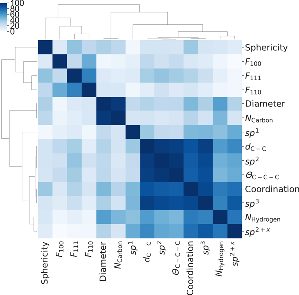
We then normalized these features and calculated the correlation matrix (Fig. 1). This confirmed that D and N _Carbon are strongly correlated, the fraction of sp ² atoms, d _C–C and Θ_C–C–C are strongly correlated, and Coord and the fraction of sp ³ atoms are strongly correlated. We therefore exclude N _Carbon, d _C–C, Θ_C–C–C, and the fraction of sp ³ (which are bulk-like); retaining D, sp ² fraction, and Coord (which are surface-like). This reduces the number of structural dimensions to 10, but it is interesting to note that the fraction of (111) surface area is not strongly correlated with the fraction of sp ² atoms, as would be typically expected based on previously published studies.^{[Reference Osswald, Yushin, Mochalin, Kucheyev and Gogotsi17,Reference Ginés, Mandal, Ahmed, Cheng, Sow and Williams18]}

Figure 1.

Hierarchical cluster map of the materials’ features describing the diamond nanoparticles after the removal of outliers, NaNs, and secondary features.

Dimension reduction

We then used these remaining structural features to train SOMs on 500 × 500 grids over five epochs; reducing the dimensionality to 2, and facilitating the visualization of the results in a scatter plot. The grid size is a hyper-parameter that determines the available number of possible neurons for matching. Too few and data are poorly mapped, and too many increases the computational cost. Given that every nanoparticle (or row/observation) gets mapped to the winning neuron (or BMUs) in the SOM and its influence spreads to neighboring neurons, the grid size is typically approximately commensurate with number of samples (nanoparticles). We tested values around this size and found that a grid size of 500 × 500 reduced the amount of overlap of the data points (giving them a better spread of possible BMUs) and aided in visualization and interpretation, without significantly increasing the computational cost.

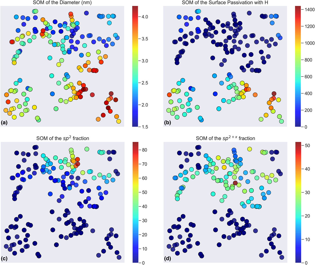
The final distribution of the points reflects the degree of similarity of each structure in 10-dimensional structure space; adjacent points are very similar, and separated points are very different. To appreciate how some important structural features are mapped on to this manifold we can encode each point with a color representing the actual magnitude of the structural feature prior to normalization. This has been done for four important features: the diameter (in nm), the number of surface hydrogen atoms, the fraction of sp ² atoms, and the fraction of sp ^2+x atoms (Fig. 2). All of these features describe surface effects, including the diameter which is a convenient measure of size related to the surface-to-volume ratio.

Figure 2.

SOMs of the 10-dimensional diamond nanoparticle data set after the removal of strongly correlated features, encoded by the absolute value of the diameter (a), the number of surface hydrogen atoms (b), fraction of sp ² hybridized atoms (c), and fraction of sp ^2+x hybridized atoms (d).

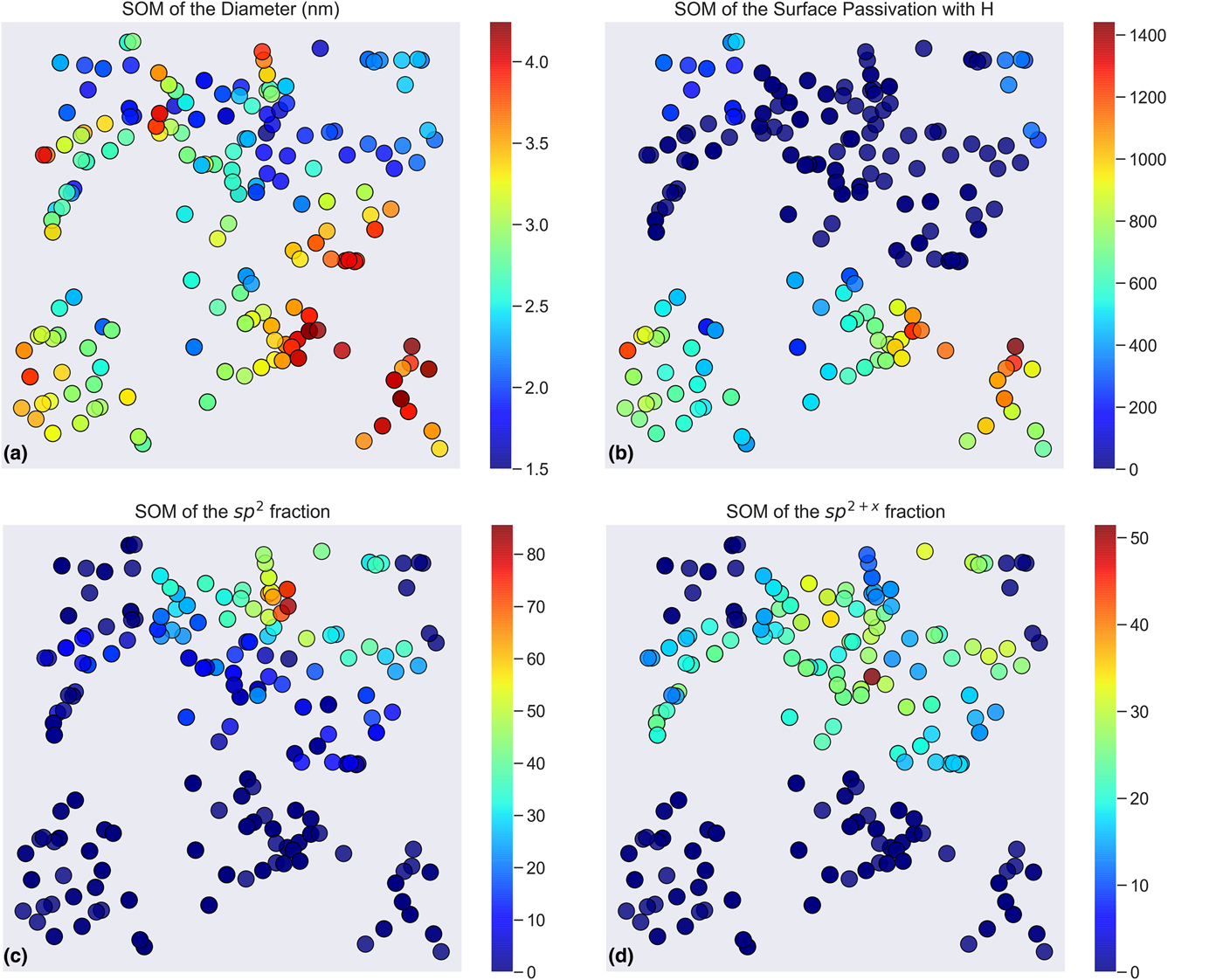
From Fig. 2 we can see that the large nanoparticles do not tend to be mapped together, which is counterintuitive for a community that often thinks in terms of size-dependent structure/property relationships. The fraction of sp ² and sp ^2+x atoms are however mapped to the same region of the space (recalling that SOMs have periodic boundary conditions), and exhibit similar relationships, though the distribution is not reflected by the size or the surface hydrogenation. More SOM feature distributions are provided for comparison in the supplemental information, where we can see that the features displayed in Fig. 2 are distributed very differently to the fraction of different surface facets, the local bonding arrangements, and the overall sphericity or under-coordination of the particles.

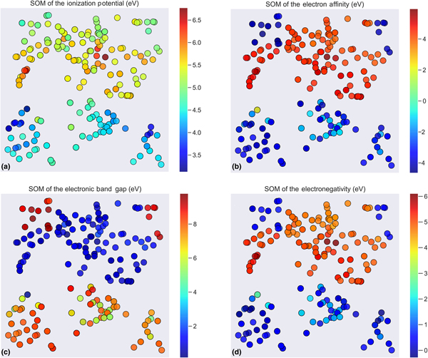
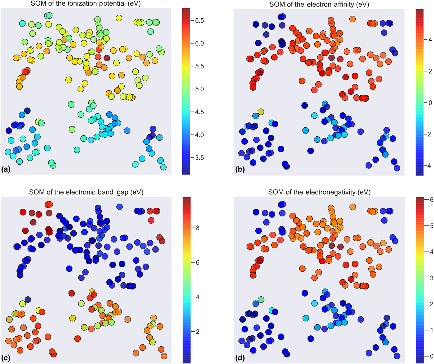
In addition to visualizing the feature space we can also encode the SOMs by the target labels (the properties, in our structure/property relationships), specifically the four charge transfer properties (Fig. 3). Here we can see that the electron affinity, electronic band gap, and the electronegativity present very similarly. The distribution of the electronic band gap and the electronegativity in 10-dimensions are almost identical, with the maps differing only by the scale of the encoded properties. When we compare these property labels (Fig. 2) to the features highlighted in Fig. 1 we can see that the electron affinity, electronic band gap, and the electronegativity are clearly related to the fraction of sp ^2+x hybridized atoms, not to the size or sp ² content as is usually assumed. Comparing with other feature (structure) maps and label (property) maps contained in the supplemental information also confirms that these properties are not strongly associated with the fraction of different types of surface facets or the overall nanoparticle shape, which has also been previously assumed. The probability of observation (provided in the supplemental information) is however, clearly related to the diameter, which is consistent with the fact that larger nanoparticles are more stable.

Figure 3.

SOMs of the 10-dimensional diamond nanoparticle data set after the removal of strongly correlated features, encoded by the absolute value of the energy of the ionization potential (a), electron affinity (b), electronic band gap (c), and electronegativity (d).

Feature importance

To confirm the relationship between the fraction of sp ^2+x hybridized atoms and the charge transfer properties we undertook regression using a random forest (RF) regressor, which is a meta estimator that fits a number of classifying decision trees on sub-samples of the data set and averages them to improve accuracy and avoid over-fitting.^{[Reference Ho19]} We have used 100 estimators with a minimum of two split samples, and bootstrapping to randomly select features to build trees and reduce problems with feature multi-collinearity. A fivefold cross validation was used to confirm the accuracy and generality of the model, with 80% of the data used for training and 20% for testing. While other regression algorithms are available and could also be applied, this regressor is particularly well suited to our problem since the data set has a high variance and we know from the input data set that we have different types of nanoparticles (twinned/un-twinned, passivated/reconstructed, etc.) that will likely all coexist in real diamond nanoparticle powders.

The RF regressor achieved excellent results for the testing (training) sets, as measured using the R ² scores. For the ionization potential we obtained testing (training) values of R ² = 0.906 (0.899); for the electron affinity we obtained R ² = 0.963 (0.947); for the band gap we obtained R ² = 0.948 (0.933); and for the electronegativity R ² = 0.966 (0.955). When we examine the importance of each feature used in the RFs we find that the regression confirms the structure/property relationships uncovered by the SOMs. Figure 4 shows the feature importance histograms for the RF of each charge transfer property.

Figure 4.

Histograms of the importance of the 10 features in predicting the energy of the ionization potential (a), electron affinity (b), electronic band gap (c), and electronegativity (d) of diamond nanoparticle, predicted using the RF regressor.

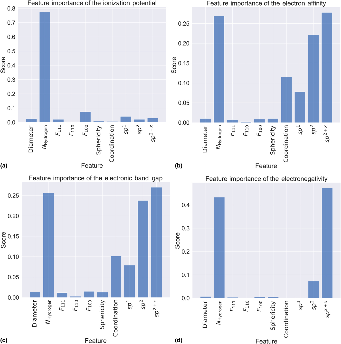
The feature importance histograms provide three important findings. First, in agreement with the SOMs, the fraction of sp ^2+x hybridized atoms is an important feature in controlling all of the charge transfer properties, with the exception of the ionization potential (again, in agreement with the SOMs). Second, that we can confidently reduce the number of dimensions to three or less, since the number of hydrogen atoms, the fraction of sp ² hybridized atoms and sp ^2+x hybridized atoms dominate the models and will be sufficient to form the basis of structure/property relationships. These are all surface features. While the importance of sp ^2+x hybridized atoms has been largely overlooked in the literature to date (which has tended to focus on sp ² hybridized atoms or surface functionalization), the importance of these three materials features is generally consistent with over a decade of domain knowledge,^{[Reference Williams, Hees, Dieker, Jäger, Kirste and Nebel20,Reference Nagl, Hemelaar and Schirhagl21]} suggesting that the ability to either passivate the surfaces or moderate the type and extent of surface reconstructions is paramount. Finally, these machine-learning results also highlight that the Diameter of the nanoparticle is not an important driver of performance, indicating that the costly production of size-selected, monodispersed samples (whether from synthesis or post-synthesis purification) is not necessary. As the size is related to the surface-to-volume ratio (and is often used as a proxy for this more appropriate nanoscale indicator) smaller particles are still desirable, but only implicitly because they expose more surface area, not because the explicitly measured diameter is low. A distribution of sizes will not inhibit performance provided the sp ² and sp ^2+x atoms are maximized.