1. Introduction
Stellarators have many desirable properties for future fusion power plants, including the ability to produce steady-state plasmas that are free of disruptions and highly stable. However, unlike tokamak devices that rely on both planar coils and large plasma current to provide rotational transform, optimized stellarators generally possess three-dimensional non-planar coils in order to generate adequate confinement. Difficulties constructing coils led to significant delays in the W7-X experiment (Riße et al. Reference Riße2009) and the cancellation of the NCSX experiment at PPPL (Neilson et al. Reference Neilson, Gruber, Harris, Rej, Simmons and Strykowsky2010).
One challenge of designing coils for modern stellarators is finding a coil set that balances the often competing goals of accurately producing a desired magnetic configuration, and satisfying various engineering constraints. These engineering constraints include designing coils that can be reasonably built, as well as ensuring that adequate space exists between coils for support structures, auxiliary systems and diagnostics. This paper focuses on one specific degree of freedom in coil design, the orientation of the coil winding pack. By optimizing the winding pack orientation, it is possible to reduce boundary errors while including engineering objective functions.
To better motivate the engineering constraints, we note some important design considerations relevant to stellarator coils. In general, engineering constraints include minimizing or eliminating sharp bends and ‘twisting’ in the conductors to avoid complications in coil fabrication and performance. Bending introduces an effect referred to as keystoning, where the conductor thins in the plane parallel to the coil and expands in the perpendicular direction. Twisting causes a warping effect that distorts the conductor. Both effects introduce difficulties when laying the conducting material into an efficient winding pack. Voids and sharp points within the coil due to bending and twisting can provide failure points under load, and therefore should be avoided to maintain structural integrity.
Modern stellarator experiments have addressed coil design in a two-stage optimization process. First, a plasma boundary is optimized for physics properties (Nührenberg and Zille Reference Nührenberg and Zille1988; Grieger et al. Reference Grieger1992; Zarnstorff et al. Reference Zarnstorff, Berry, Brooks, Fredrickson, Fu, Hirshman, Hudson, Ku, Lazarus and Mikkelsen2001; Ku et al. Reference Ku, Garabedian, Lyon, Turnbull, Grossman, Mau and Zarnstorff2008; Drevlak et al. Reference Drevlak, Brochard, Helander, Kisslinger, Mikhailov, Nührenberg, Nührenberg and Turkin2013, Reference Drevlak, Beidler, Geiger, Helander and Turkin2018; Bader et al. Reference Bader, Drevlak, Anderson, Faber, Hegna, Likin, Schmitt and Talmadge2019; Henneberg et al. Reference Henneberg, Drevlak, Nührenberg, Beidler, Turkin, Loizu and Helander2019). The result of this optimization is typically a target configuration that is identified by a boundary surface. The second stage of the design is producing a coil set that best matches the desired boundary surface (Merkel Reference Merkel1987; Drevlak Reference Drevlak1998; Strickler et al. Reference Strickler, Berry and Hirshman2002; Landreman Reference Landreman2017; Zhu et al. Reference Zhu, Hudson, Song and Wan2017; Paul et al. Reference Paul, Landreman, Bader and Dorland2018; Zhu et al. Reference Zhu, Hudson, Song and Wan2018). Typically, this is done by specifying filamentary coils as an approximation to coils with a finite-build structure. This paper describes an additional step to the design, namely extending the precomputed filamentary coils to coils with finite builds, represented by multiple filaments (‘multi-filaments’) in a rectangular array. An additional optimization procedure is undertaken which seeks to orient the array of filaments to best reproduce the target boundary.
Before the optimization of the multi-filament orientation is considered, some explanation of how the filamentary coils are determined is necessary. The magnetic field produced by currents in the external coil set, termed the vacuum field  $\boldsymbol {B_v}$, must balance the magnetic field
 $\boldsymbol {B_p}$ produced by currents present in the plasma so that the normal component of the total magnetic field
 $\boldsymbol {B} = \boldsymbol {B_v} + \boldsymbol {B_p}$ on the plasma boundary is zero. The vacuum field is typically computed using the Biot–Savart law, and
 $\boldsymbol {B_p}$ is held constant throughout the optimization. The boundary is typically specified in terms of Fourier harmonics
 $R_{mn}$ and
 $Z_{mn}$ over poloidal angle
 $\theta$ and toroidal angle
 $\zeta$ as,
 \begin{gather} R(\theta,\zeta) = \sum_{m,n}R_{mn}\cos(m\theta-n\zeta), \end{gather}
 \begin{gather}Z(\theta,\zeta) = \sum_{m,n}Z_{mn}\sin(m\theta-n\zeta), \end{gather}
where stellarator symmetry, i.e.  $R(\theta , \zeta ) = R(-\theta , -\zeta );\ Z(\theta , \zeta ) = -Z(-\theta , -\zeta )$, is enforced for convenience. Some coil-design tools can optimize coils for both physics requirements and engineering constraints (Drevlak Reference Drevlak1998; Strickler et al. Reference Strickler, Berry and Hirshman2002), but to date, all existing optimization codes ultimately produce zero-thickness filaments. Optimized stellarators, such as Helically Symmetric eXperiment (HSX), have been built with finite-sized coils. These previous efforts often only used simple engineering constraints, such as coil clearances, to determine coil shapes. For the design of HSX, the NESCOIL code (Merkel Reference Merkel1987) solved for the current potential lines on a set of nested topologically toroidal surfaces. A linear fit was computed across shells (with increased weight on the innermost shell) to derive one axis of the winding pack. Manual adjustments were made as needed to eliminate coil intersections.
The description of the second coil optimization, that of the multi-filament coils, is specified in the rest of this paper. The details of the algorithm to generate optimized multi-filament coils are presented in § 2. A new tool, optimization of multi-filament coils (OMIC), is introduced in § 3. Sections 4 and 5 present example applications and discuss comparisons of optimized and unoptimized multi-filament coils. Finally, conclusions and future work are discussed in § 6.
2. Filament optimization
2.1. The single-filament model
The multi-filament coil optimization presented in this paper employs many of the same techniques used for single-filament optimization. Furthermore, in order to optimize multi-filament coils in the current framework, a single-filament representation needs to be obtained first. An explanation of the single-filament optimization, as used in FOCUS (Zhu et al. Reference Zhu, Hudson, Song and Wan2018), is given in this section. A Fourier series representation for single-filament coils in three-dimensional space is employed. This representation produces smooth coils and has the advantage of simple analytic derivatives. The explicit formulation is given by,
 \begin{equation} \boldsymbol{r}(\phi) = {\boldsymbol{X_{c,0}}} + \sum_{n=1}^{N_{F}} \left[{\boldsymbol{X_{c,n}}}\cos(n\phi) + {\boldsymbol{X_{s,n}}}\sin(n\phi)\right], \end{equation}
where  $\boldsymbol {r}(\phi ) = x(\phi )\boldsymbol {\hat {x}}+y(\phi )\boldsymbol {\hat {y}}+z(\phi )\boldsymbol {\hat {z}}$ is the position vector of the filament, and
 ${\boldsymbol {X_{c,0}}}$ is the centroid of the coil. Here,
 ${\boldsymbol {X_{c,n}}}$ and
 ${\boldsymbol {X_{s,n}}}$ are cosine and sine Fourier coefficients for mode number
 $n$. These coefficients can be combined into the optimization vectors
 $\boldsymbol {X_c}$ and
 $\boldsymbol {X_s}$, which are vectors of
 $N_F+1$ cosine terms and
 $N_F$ sine terms. Because there are individual coefficients for each Cartesian coordinate, for a given maximum mode number
 $N_F$ there are
 $6N_F+3$ independent variables in the optimization of each coil. In these expressions,
 $\phi$, which varies from
 $0$ to
 $2{\rm \pi}$, is a variable that parameterizes the filament.
2.2. Target functions
This paper includes results from a new quasihelically symmetric configuration. In order to carry out the multi-filament analysis, an optimized set of single-filament coils was generated by varying the coefficient vectors  $\boldsymbol {X_{c}}$ and
 $\boldsymbol {X_{s}}$ in FOCUS. Three targets were used to optimize the single-filament coils. The most important metric, and the main metric we will use to judge multi-filament coils, is how well the coils match a desired field on the plasma boundary. Since the normal field on the boundary should be exactly zero everywhere, the squared relative error of the integrated normal field
 $f_B$ on the boundary surface
 $S$,
 \begin{align} f_B(\boldsymbol{X_c},\boldsymbol{X_s}) \equiv \left[ \frac{1}{2} \int_{S} \left( \frac{\boldsymbol{B} \boldsymbol{\cdot} \boldsymbol{n}}{\lvert \boldsymbol{B} \rvert} \right)^2 \textrm{d} s \right] \left( \int_S \textrm{d} s \right)^{-1}, \end{align}
is minimized. As before,  $\boldsymbol {X_c}$ and
 $\boldsymbol {X_s}$ represent the cosine and sine coefficients of the single-filament coils. Here,
 $\boldsymbol {n}$ is a normal vector to the boundary surface
 $S$, and therefore
 $\boldsymbol {B} \boldsymbol {\cdot } \boldsymbol {n}$ is the value of the normal field. The quantity
 $\int _S \textrm {d} s$ is the surface area of the boundary. Because an equilibrium surface perfectly matched by coils has zero normal field everywhere on the plasma boundary, finite values of the normal field represent deviations from the target equilibrium.
Additional target functions are also employed to constrain the single-filament coils. One target function penalizes deviations from prescribed target lengths,
 \begin{gather} f_{L} \equiv \frac{1}{N_c}\sum_{i=1}^{N_c} \frac{1}{2}\frac{\left( L_i - L_{i,0} \right)^2}{L_{i,0}^2}, \end{gather}
 \begin{gather}L_i=\int_0^{2{\rm \pi}} \left | \frac{\textrm{d} \boldsymbol r}{\textrm{d} \phi} \right | \textrm{d} \phi, \end{gather}
where  $N_c$ is the number of unique coils,
 $L_i$ is the length of a given coil and
 $L_{i,0}$ is the target length of the coil. An optimization procedure often requires adjusting the
 $L_{i,0}$ values through successive iterations. For a given coil, a larger
 $L_{i,0}$ tends to increase coil–plasma distance, which is desirable, but also tends to add additional wiggles and toroidal excursions to the coil, which is undesirable.
The third function provides limits on coil curvature. The curvature target is given as,
 \begin{gather} f_{\kappa} \equiv \frac{1}{N_c}\sum_{i=1}^{N_c} \int_0^{2{\rm \pi}}c\left(\kappa_i(\phi)-\kappa_0 \right)^\gamma\textrm{d}\phi;\quad c\left(\kappa, \kappa_0\right) = \left\{\begin{matrix} 1 & \mathrm{if}\ \kappa_i \ge \kappa_0\\ 0 & \mathrm{if}\ \kappa_i < \kappa_0\\ \end{matrix}\right. \end{gather}
 \begin{gather}\kappa_i = \frac{|{\boldsymbol r}' \times {\boldsymbol r}''|}{|{\boldsymbol r}'|^3}, \end{gather}
where  $\kappa _i$ is the local curvature at the point
 $\boldsymbol {r}(\phi )$ along the coil, and primes denote differentiation with respect to
 $\phi$. The Heaviside function,
 $c$, ensures the coil is only penalized for locations where the curvature exceeds some predetermined value
 $\kappa _0$, usually set by engineering constraints. For the optimizations here,
 $\kappa _0$ is set to 10 m
 $^{-1}$ for all coils, setting a minimum radius of curvature of 10 cm. These optimizations use
 $\gamma =2$ although values of
 $\gamma > 2$ are also acceptable.
The total penalty function is,
 \begin{equation} f=w_{B}\,f_{B}+w_{L}\,f_{L}+w_{\kappa}\,f_{\kappa}, \end{equation}
where the weights  $w_B$,
 $w_L$ and
 $w_\kappa$ are set by the user to guide the optimizer in different directions. FOCUS can optimize filaments using various descent algorithms, including the nonlinear conjugate gradient method. Fast calculation of target function derivatives with respect to the coil coefficients is available using analytic derivatives. More details can be found in Zhu et al. (Reference Zhu, Hudson, Song and Wan2018).
2.3. A multi-filament coil model
The multi-filament coil representation is motivated by the internal structure of non-superconducting modular stellarator coil sets, including those of W7-AS and HSX (Sapper and Renner Reference Sapper and Renner1990; Anderson et al. Reference Anderson, Almagri, Anderson, Matthews, Talmadge and Shohet1995). These coils are comprised of  $N_W$ layered windings each containing
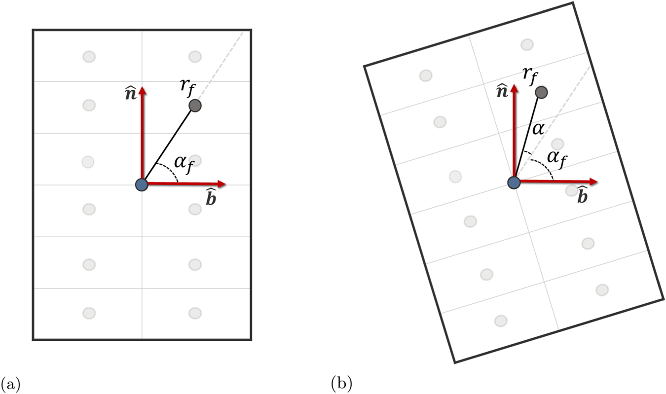
 $N_{T}$ turns, producing a rectangular array referred to as the ‘winding pack’. In the multi-filament representation, each space of the array is represented as a filament, producing a two-dimensional rectangular array of
 $N_W \times N_{T}$ parallel filaments. To place the set of filaments in space, we centre the winding pack about the single-filament coil. User-specified winding pack dimensions then determine the location of each parallel filament relative to the central single-filament coil, which can be expressed in terms of distance
 $r_f$, angle
 $\alpha _f$ and angle of orientation of the winding pack
 $\alpha$, as shown in figure 1. In the plane of the winding pack, the coordinates of filament
 $f$ are given by,
 \begin{gather} x_f = r_f\cos\left(\alpha +\alpha_f\right) \end{gather}
 \begin{gather}y_f = r_f\sin\left(\alpha + \alpha_f\right). \end{gather}
The first two parameters,  $r_f$ and
 $\alpha _f$, are held fixed for each filament. The third parameter,
 $\alpha$, is a free parameter and can vary at each point along the coil. Optimization of
 $\alpha$ is the main focus of this paper, so we refer to it as the optimization angle.
(a) Schematic of a coil winding pack with  $N_W = 2$ and
 $N_T=6$. Each filled circle represents a filament comprising the multi-filament coil. The central filled circle, shown in blue, represents the corresponding single-filament coil. The orientation of the winding pack is determined by the normal and binormal vectors. The coordinates of one filament are given by
 $r_f$ and
 $\alpha _f$. (b) The effect of the optimization angle
 $\alpha$ on winding pack given in (a). The dashed grey line indicates the initial filament direction prior to rotation.

2.4. The Frenet–Serret frame
There is no unique orthogonal basis local to the filament  $f$ even if one of the axes, such as the
 $z$ axis, is taken to be the tangent direction. Therefore, a choice must be made regarding how to orient the axes that are normal to the tangent vector. The three orthogonal axes are referred to as the local winding pack coordinate frame, and it suffices to specify a single parameter to define the relative orientation of the
 $x$- and
 $y$-axes in this frame.
One choice for the local winding pack coordinate frame is given by the Frenet–Serret formulas. In terms of the coil parameterizing variable  $\phi$ these are,
 \begin{gather} \boldsymbol{\hat{t}}_{fs} = \frac{{\partial \boldsymbol{r}} / {\partial \phi}}{\lvert{\partial \boldsymbol{r}} / {\partial \phi}\rvert}, \end{gather}
 \begin{gather}\boldsymbol{\hat{n}}_{fs} = \frac{{\partial \boldsymbol{\hat{t}}} / {\partial \phi}}{\lvert{\partial \boldsymbol{\hat{t}}} / {\partial \phi}\rvert}, \end{gather}
 \begin{gather}\boldsymbol{\hat{b}}_{fs} = \boldsymbol{\hat{t}} \times \boldsymbol{\hat{n}}, \end{gather}
where, as before,  $\boldsymbol {r}$ is the curve given by (2.1). The normal
 $\boldsymbol {\hat {n}_{fs}}$ and binormal
 $\boldsymbol {\hat {b}_{fs}}$ directions to the curve could then specify the two unique winding pack directions. Simple and fully analytic expressions for the Frenet–Serret frame given by (2.10)–(2.12) can be derived from (2.1) and can be readily implemented into any optimization procedure.
There is an inherent limitation to the use of the Frenet–Serret frame. If a filament has a vanishing value of  $\partial \boldsymbol {\hat {t}}_{fs} / {\partial \phi }$ then the normal vector,
 $\boldsymbol {\hat {n}_{fs}}$ is undefined. This will happen whenever the coil is locally straight. Even if the coil is only approximately straight, that is, regions where
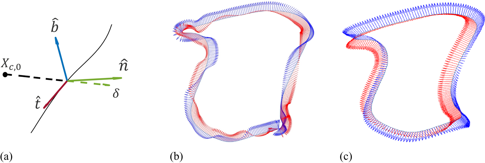
 $\partial \boldsymbol {\hat {t}}_{fs} / {\partial \phi } \ll 1$, the local normal and binormal angle can oscillate strongly over a short distance, producing complicated coil shapes. This behaviour can be seen in figure 2(b,c). Figure 2(b) shows Frenet–Serret basis vectors along an example coil. In the bottom right of the figure the value of
 $\partial \boldsymbol {\hat {t}}_{fs} / {\partial \phi }$ is small and the vectors display rapid variation. Figure 2(c) shows an alternative to the Frenet–Serret frame that reduces these variations. This will be the topic of § 3.1.
(a) Visual representation of the coil centroid coordinate frame. Basis vectors are shown at one position along a single-filament coil. (b) Frenet–Serret frame normal  $\boldsymbol {\hat {n}}_{fs}$ (red) and binormal
 $\boldsymbol {\hat {b}}_{fs}$ (blue) vectors for an example stellarator coil. (c) Coil centroid frame normal
 $\boldsymbol {\hat {n}}$ and binormal
 $\boldsymbol {\hat {b}}$ vectors for an example stellarator coil.

3. Optimization of multi-filament coils
3.1. A coil centroid frame
An alternative local coordinate frame that does not vary rapidly at straight sections of the single-filament curve has been identified. We modify the definition of the Frenet–Serret normal vector while retaining the definition of the tangent and binormal vectors. First, the coil centroid  $\boldsymbol {R}$ is computed as,
 \begin{equation} \boldsymbol{R} = \frac{1}{2{\rm \pi}}\int_{0}^{2{\rm \pi}} \boldsymbol{r}(\phi) \,\textrm{d}\phi, \end{equation}
where again  $\boldsymbol {r}(\phi )$ is given by (2.1). As noted previously, this centroid is simply the constant amplitude of the Fourier series given in (2.1),
 $\boldsymbol {X_{c,0}}$. Next, a vector
 $\boldsymbol {\delta }(\phi )$ pointing from
 $\boldsymbol {X_{c,0}}$ to position
 $\boldsymbol {r}(\phi )$ is computed as
 $\boldsymbol {\delta }(\phi ) = \boldsymbol {r}(\phi ) - \boldsymbol {X_{c,0}}.$ The component of
 $\boldsymbol {\delta }(\phi )$ orthogonal to the tangent vector at
 $\boldsymbol {r}(\phi )$ is then found via the Gram–Schmidt process. The resulting normal vector is found by normalizing the component of
 $\boldsymbol {\delta }$ orthogonal to the tangent vector. The tangent vector and binormal vectors retain their definitions, giving the coordinate frame,
 \begin{gather} \boldsymbol{\hat{t}} = \frac{{\partial \boldsymbol{r}} / {\partial \phi}}{\lvert{\partial \boldsymbol{r}} / {\partial \phi}\rvert} \end{gather}
 \begin{gather}\boldsymbol{\hat{n}} = \frac{ \boldsymbol{\delta} - (\boldsymbol{\delta} \boldsymbol{\cdot} \boldsymbol{\hat{t}})\boldsymbol{\hat{t}}} {\lvert \boldsymbol{\delta} - (\boldsymbol{\delta} \boldsymbol{\cdot} \boldsymbol{\hat{t}})\boldsymbol{\hat{t}} \rvert}, \end{gather}
 \begin{gather}\boldsymbol{\hat{b}} = \boldsymbol{\hat{t}} \times \boldsymbol{\hat{n}}. \end{gather}
The coil centroid frame at one location along a filament coil is shown in figure 2(a).
By analogy with the Frenet–Serret formulas, the modified normal and corresponding binormal directions specify the winding pack orientation of the finite coil. The vector  $\boldsymbol {\delta }(\phi )$ is expected to be well defined everywhere along the single-filament curve, so this coordinate frame should not suffer from rapid rotation at single-filament straight sections, unlike the Frenet–Serret frame. This is not true in the specific case where a coil segment is oriented parallel to a ray originating from the coil centroid. Such coil segments are avoided in the calculations presented in this paper. The coil centroid frame normal and binormal vectors are shown in figure 2(c). In this figure, the smooth variation of the normal and binormal vectors over the entire coil length is visible.
3.2. Initial multi-filament HSX coils
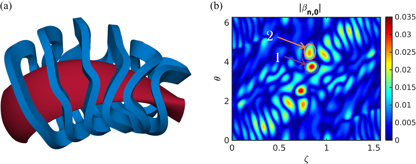
Figure 3(a) shows the coils produced by expanding filaments using the normal and binormal directions from the coil centroid frame for the HSX device. Only a half-period is shown, with all six distinct coils. In the HSX device, these coils would be mirrored to produce the corresponding set for a full period. For these coils, a winding pack with  $N_W=2$ and
 $N_T=7$ is used with cross-section dimensions of 6 by 12 cm, similar to the actual HSX coil dimensions. Figure 3(b) shows the value of the normal magnetic field divided by the field strength, which we will refer to as the normal field error,
 $|\boldsymbol {\beta _n}| = |\boldsymbol {B_n}|/|\boldsymbol {B}| = (\boldsymbol {B} \boldsymbol {\cdot } \boldsymbol {n})/|\boldsymbol {B}|$ on the boundary for one full period. Stellarator symmetry is visible in the plot by inspection:
 $|\boldsymbol {\beta _n}(\theta , \zeta )| = |\boldsymbol {\beta _n}(2{\rm \pi} -\theta , 2{\rm \pi} /N-\zeta )|$, where
 $N$ is the number of periods, 4 for HSX. This unoptimized case is used as a baseline for comparing the HSX-like coil optimizations discussed in the rest of the paper. As such, the normal field error for this case is referred to as
 $|\boldsymbol {\beta _{n,0}}|$ with the ‘0’ subscript indicating the baseline scenario.
(a) The HSX coils with winding pack orientation ( $r_f$,
 $\alpha _f$) given by the coil centroid frame are shown in blue, with the plasma boundary in red. (b) The magnitude of the normal magnetic field error on the boundary as a function of toroidal angle
 $\zeta$ and poloidal angle
 $\theta$ for the coils given in (a). Two hotspots with large values of
 $|\boldsymbol {\beta _{n,0}}|$ are pointed out in the plot, hotspot 1 in purple and hotspot 2 in orange.

As can be seen in figure 3(b), the largest local errors on the boundary are approximately 3.5 %, and these correspond to the half period,  $\zeta = {\rm \pi}/4$. This is also the location where the coils have the largest toroidal excursions. The expectation is that this is the area where optimization can have the largest effect, but possibly at the expense of making already complicated coils even more complicated. Specifically we will focus on 2 ‘hotspots’ near
 $\zeta = {\rm \pi}/4$ that are labelled in figure 3(b). Hotspot 1 has the largest error on the boundary with
 $|\boldsymbol {\beta _{n,0}}| \approx 3.5\,\%$. Hotspot 2 has a normal field error of
 $|\boldsymbol {\beta _{n,0}}| \approx 2.5\,\%$. Both hotspots appear in two separate stellarator-symmetric locations. The half-period where the hotspots appear tends to be one of the more difficult to match for quasihelically symmetric configurations because at the half-period, the high-field side is on the outside of the device, and the low-field side is on the inside. Both are difficult to match, but the fact that the hotspots are located close to
 $\theta ={\rm \pi}$ in figure 3(b) indicates that it is the low field on the inboard side that is the more difficult to replicate for this coil set.
3.3. Optimization of winding pack rotation profile
Single-filament coil sets, multi-filament coil sets with orientation determined using the Frenet–Serret frame (2.10)–(2.12) and multi-filament coil sets with orientation determined using the coil centroid frame (3.2)–(3.4) all produce different plasma boundaries. Because the orientation of the winding pack itself is a free parameter for the construction of the coils, it can be optimized to determine which orientation best reproduces the target boundary. To allow the flexibility to optimize the rotational profile, we introduce the scalar function  $\alpha (\phi )$ defined along each multi-filament coil in a set. This function is represented as the Fourier series,
 \begin{equation} \alpha(\phi) = \alpha_{c,0} + \sum_{n=1}^{N_{\alpha}}\left[\alpha_{c,n}\cos(n\phi) + \alpha_{s,n}\sin(n\phi)\right], \end{equation}
where, analogous to (2.1),  $\alpha _{c,n}$ and
 $\alpha _{s,n}$ are the cosine and sine Fourier coefficients. The effect of this function is, at each single-filament position
 $\boldsymbol {r}(\phi )$, a local rotation of the winding pack by
 $\alpha =\alpha (\phi )$, as can be seen in figure 1. All
 $N_\alpha + 1$ cosine and
 $N_\alpha$ sine coefficients can be combined into the optimization vector
 $\boldsymbol {A}$ with
 $N_c(2N_\alpha + 1)$ independent variables.
To limit the twisting of optimized coils, particularly at high values of  $N_{\alpha }$, a spectral weighting is added to the optimization procedure in OMIC. High-order modes in the Fourier series (3.5) are penalized by the function,
 \begin{equation} f_{\mathrm{sw}}(\boldsymbol{A}) = \sum_{i} A_i^2 n_i^2, \end{equation}
where  $A_i$ is the
 $i$th coefficient of
 $\boldsymbol {A}$ and
 $n_i$ is the mode number corresponding to
 $A_i$. The objective function implemented in OMIC is the weighted sum of both (2.2) and this spectral weighting cost function,
 \begin{equation} f(\boldsymbol{A}) = w_{B}f_{B}(\boldsymbol{A}) + w_{\mathrm{sw}}f_{\mathrm{sw}}(\boldsymbol{A}), \end{equation}
where  $w_{B}$ and
 $w_{\mathrm {sw}}$ weight the
 $f_B$ and
 $f_{\mathrm {sw}}$ cost functions, respectively. In general,
 $f_B$ is a function of
 $\boldsymbol {X_c}$,
 $\boldsymbol {X_s}$ and
 $\boldsymbol {A}$, but in this paper we vary only the coefficients in
 $\boldsymbol {A}$ and hold
 $\boldsymbol {X_c}$ and
 $\boldsymbol {X_s}$ constant.
3.4. Steepest descent method in OMIC
To determine the set of Fourier coefficients  $\boldsymbol {A}$ that best minimizes (3.7), a forward-tracking gradient descent line search is performed. The integrated normal field error cost function derivative is approximated by central differences. With respect to the
 $i$th element of
 $\boldsymbol {A}$, the central difference is,
 \begin{equation} \frac{\partial f_B}{\partial A_i} \approx \frac{f_B(A_i+h)-f_B({A_i}-h)}{2h}, \end{equation}
where  $h$ is some step. The spectral weighting cost function derivative is computed analytically and has the simple form,
 \begin{equation} \frac{\partial f_{\mathrm{sw}}}{\partial A_i} = 2 A_i n_i^2. \end{equation}
Multi-filament coils are initialized with  $\boldsymbol {A}=\boldsymbol {0}$, which is chosen to correspond with the coil centroid frame given by (3.2)–(3.4). At each iteration
 $k$ of the optimization, Fourier coefficients in
 $\boldsymbol {A}^{(k)}$ change according to,
 \begin{equation} \boldsymbol{A}^k = \boldsymbol{A}^{k-1} - p_k \boldsymbol{\nabla} f(\boldsymbol{A}^{k-1}). \end{equation}
Here,  $p_k$ is a step size and
 $\boldsymbol {\nabla }$ denotes the vector containing all
 ${\partial }/{\partial A_i}$. We note that coil current is not optimized in OMIC, as it is assumed that single-filament currents have previously been optimized. In these optimizations, each single-filament current is divided uniformly amongst the
 $N_W \times N_T$ filaments that comprise each multi-filament coil.
4. Applications
4.1. Designing coils for the HSX stellarator
The HSX is an optimized stellarator located at the University of Wisconsin-Madison (Anderson et al. Reference Anderson, Almagri, Anderson, Matthews, Talmadge and Shohet1995) that was designed in the 1980s and began operation in the early 2000s. The magnetic design of this stellarator emphasizes quasihelical symmetry such that one mode, the  $n=4$,
 $m=1$ mode, is dominant. The major radius of the device is 1.2 m, the minor radius is 0.12 m and the magnetic field on axis is 1 T. HSX is a four field period device with 12 main modular coils per period for a total of 48 coils. Due to the stellarator symmetry of the HSX configuration, there are only a total of 6 unique main coils. For the optimization, the HSX coils are represented by filaments defined as the centre of the winding pack of each actual HSX coil. These single-filament coils are then expanded into multiple filaments using the coil centroid frame. In the optimization, a winding pack with
 $N_W=2$ and
 $N_T=7$ was chosen. For these coils, the winding pack cross-section is 6 by 12 cm, which is similar to the actual HSX coils. The total coil current is 150 kA giving a current density of
 $\sim$2 kA cm
 $^{-2}$.
The finite build of the HSX coils is determined by optimizing multi-filament coils using OMIC. The results are shown in figure 4(a–c). The difference between the coil optimizations is the spectral weighting term,  $w_{\mathrm {sw}}$. The leftmost column (a, d, g, j) show the result with no spectral weighting, the rightmost column (c, f, i, l) have the highest spectral weighting, while the middle column (b, e, h, k) have intermediate weighting. In all optimization results, the number of Fourier modes in the spectrum,
 $N_\alpha$ was limited to 5. Figure 4(a) shows the coils with no spectral weighting applied. The resulting coils show very significant twists. In contrast, figure 4(c) shows a result with fairly high weighting on the spectral terms. As a result, the coils exhibit less overall rotation of the winding pack. The difference between these coils with high spectral weighting and the unoptimized coils shown in figure 3(b) is not easily visible.
OMIC optimization results for HSX-like coils. (a–c) Show the optimized coils (blue) with the plasma boundary (red). (d–f) Show the optimization angle  $\alpha$ as a function of parameterizing angle
 $\phi$ for the 6 coils. (g–i) Show the normal field error on the boundary from the coils as a function of the toroidal angle
 $\zeta$ and the poloidal angle
 $\theta$. (j–l) Show the difference between the corresponding normal field error (g–i) and the normal field error with no optimization (figure 3b). The three different coil sets examined are without spectral weighting (left), with medium spectral weighting (middle) and with high spectral weighting (right).

Figure 4(d–f) shows the rotation angle,  $\alpha$, as a function of the parameterizing angle along the coil,
 $\phi$. From here, the differences in the allowable twist is visible. In the two cases with lower spectral weighting (d, e), the rotation angle reaches almost
 ${\rm \pi} /2$ on coils 4, 5 and 6. This highlights the difficulty of matching target fields in this region. Interestingly, the
 $\alpha$ angle for coil 1 shows a large
 $n=4$ mode in the case with no spectral weighting. Without the spectral weighting, the algorithm includes high deviations for this coil for only minor benefit. Figure 4(f) shows results for coils with the highest spectral weighting, and with this set, the
 $\alpha$ angle does not exceed 0.5 on any coil. However, even with this high spectral weighting, coils 4, 5 and 6 can be seen to deviate the most.
The results from the optimization can be seen in figure 4(g–l). Plotted in (g–i) are the values of  $|\boldsymbol {\beta _n}| = |\boldsymbol {B_n}|/|\boldsymbol {B}|$, the normal field on the boundary divided by the field magnitude at that position. Recalling the positioning of the hotspots near
 $\zeta = {\rm \pi}/4$ shown in figure 3(b), it is clear that only the case with no spectral weighting (g) can effectively eliminate both hotspots. The cases with spectral weighting (h,i) can reduce only hotspot 2.
The direct improvements for all the configurations can be seen in (j–l). These figures show the difference between  $|\boldsymbol {\beta _n}|$ of the optimized coils and
 $|\boldsymbol {\beta _{n,0}}|$ of the unoptimized coils (figure 3b). In these plots, blue colours represent locations on the boundary where the optimized coils perform better, i.e. where the normal component of the magnetic field on the boundary is smaller. Conversely, red colours represent locations where the unoptimized coils perform better. Because the target function metric only considers the integrated error on the boundary, it can produce overall improvement even if the local matching is worse in some places (red) provided it improves more significantly in other places. In the case with no spectral weighting (j), both hotspots are visible as deep blue sections where large improvement occurred. Hotspot 2 is visible on the two cases with no spectral weighting (k,l), but there appears to be no improvement for hotspot 1.
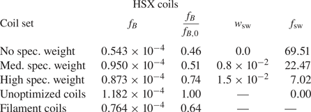
The improvements of the coils with no spectral weighting are available by inspection in figure 4(j). However, the explicit improvement in the target function can be calculated and is shown in table 1. Here the integrated normal field error  $f_B$ and spectral weighting
 $w_{{\rm sw}}$ values are given. In addition, the value of the normalized integrated field,
 $f_B/f_{B,0}$ is given, which directly compares the improvement of a given configuration with the unoptimized field. For the case without spectral weighting, the integrated normal field error is reduced by approximately half. This represents the largest possible reduction available through modifying the coil angle. However, even for fairly modest optimization of the coil angle, as evidenced by the high spectral weighting case, the integrated error can be reduced by approximately 25 %.
Values for the integrated normal field,  $f_B$; the normalized integrated field,
 $f_B/f_{B,0}$; the spectral weight,
 $w_\mathrm {sw}$, and the spectral weight penalty,
 $f_\mathrm {sw}$, for HSX-like coils with three separate spectral weights. Results are also given for the initial unoptimized coils and the corresponding filament coils.

4.2. Candidate coil designs for a new UW-Madison QHS stellarator
A new quasihelically symmetric stellarator configuration is under investigation at the University of Wisconsin-Madison, and a candidate plasma equilibrium has been found (Bader, submitted to JPP). This equilibrium, which we refer to as WISTELL-A, is optimized for physics goals, including energetic particle confinement, neoclassical transport and magnetohydrodynamic stability. WISTELL-A has a major radius of 2.0 m, a minor radius of 0.3 m and a magnetic field strength on axis of 2.5 T. Like HSX, WISTELL-A is a four field period device with 12 main modular coils per period, 6 of which are unique. Single-filament coils for WISTELL-A have been optimized to maximize coil–plasma distance using the procedures described in § 2.2. In the optimization, a winding pack with  $N_W=2$ and
 $N_T=7$ was chosen. For these coils, the winding pack cross-section is 7.5 by 15 cm. The coil current is 590 kA, producing a higher current density (
 $\sim$5 kA cm
 $^{-2}$) than the low current density used in the HSX coils, which was mainly chosen due to power supply limitations. The normalized boundary error
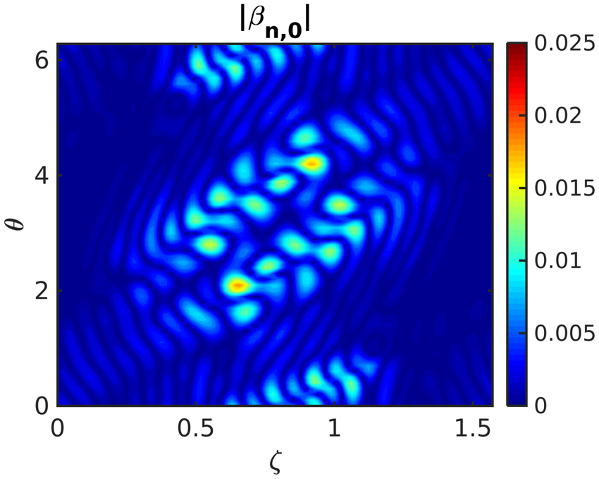
 $|\boldsymbol {\beta _{n,0}}|$ corresponding to this coil set is shown in figure 5.
The magnitude of the normal magnetic field error on the boundary as a function of toroidal angle  $\zeta$ and poloidal angle
 $\theta$ for the WISTELL-A unoptimized coils initialized using the coil centroid frame.

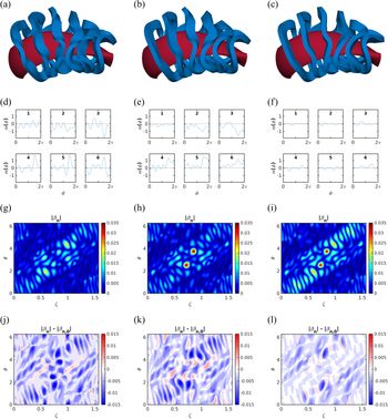
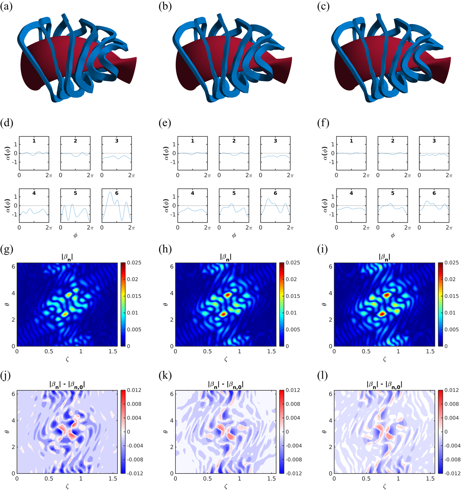
The results of the multi-filament coil optimizations are shown in figure 6. The layout is similar to figure 4 in that the top row shows the coils, the second row plots the optimization angle  $\alpha$ as a function of parameterizing angle
 $\phi$, the third row shows the values of
 $|\boldsymbol {\beta _n}|$ on the boundary and the bottom row shows the difference in the normal magnetic field between the optimized and unoptimized coils. As before, the leftmost column shows the results where there is no spectral weighting on
 $\alpha _n$ values, and the rightmost column has the largest spectral weighting. Like the HSX results, unoptimized coils for this case refer to those initialized using the coil centroid frame.
OMIC optimization results for WISTELL-A coils. (a–c) Show the optimized coils (blue) with the plasma boundary (red). (d–f) Show the optimization angle  $\alpha$ as a function of parameterizing angle
 $\phi$ for the 6 coils. (g–i) Show the normal field error on the boundary from the coils as a function of the toroidal angle
 $\zeta$ and the poloidal angle
 $\theta$. (j–l) Show the difference between the corresponding normal field error (g–i) and the normal field error with no optimization (figure 5). The three different coil sets examined are without spectral weighting (left), with medium spectral weighting (middle) and with high spectral weighting (right).

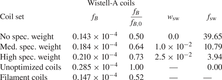
Some similarities with the HSX coils are easily visible. Most obvious is that, as with HSX, the largest errors on the boundary are near the half-period. Furthermore, the coils at this period tend to also have the largest variation in the  $\alpha$ angle. However, unlike in HSX, these variations are not large enough to completely remove the areas with largest
 $|\boldsymbol {\beta _{n}}|$, as can be seen by comparing figure 5 with 6(g). When examining the values of the normal integrated field error in table 2, it can be seen that the same overall level of improvement is obtained by optimizing the WISTELL-A coils as was found when optimizing the HSX coils. That is, the case with no constraints on the spectral weighting found roughly a 50 % improvement, while the high spectral weighting case found roughly a 25 % improvement.
Values for the integrated normal field,  $f_B$; the normalized integrated field,
 $f_B/f_{B,0}$; the spectral weight,
 $w_\mathrm {sw}$, and the spectral weight penalty,
 $f_\mathrm {sw}$, for Wistell-A coils with three separate spectral weights. Results are also given for the initial unoptimized coils and the corresponding filament coils.

5. Discussion
5.1. Dependence on single-filament optimization
In both the HSX and WISTELL-A coil sets, the agreement between the vacuum field due to the coils and the desired plasma boundary, as measured by the integrated normal field, worsens with spectral weighting. The relative improvements for the cases with no spectral weighting and the cases with high spectral weighting are approximately the same in both HSX and WISTELL-A. This can be seen numerically by the  $f_B/f_{B,0}$ column of tables 1 and 2. However, figures 4(g–i) and 6(g–i) show the maximum
 $|\boldsymbol {\beta _n}|$ error among all optimized coil sets differs by about a factor of two between the configurations. The maximum error is roughly 2.5 % in the HSX coil sets and 1.2 % in the WISTELL-A coil sets. Part of this difference can be attributed to differences in the single-filament coil set that corresponds with each configuration. The WISTELL-A coils were explicitly designed with new modern tools to increase coil–plasma spacing, thus reducing coil ripple, one of the main sources of error. The average coil-plasma distance for the filamentary WISTELL-A coils is
 $\sim$22.5 cm. In contrast, the HSX coils were designed with an early code, NESCOIL, that enforced a constant, and relatively small coil–plasma spacing,
 $\sim$14.5 cm for the filamentary coils. Partly for this reason, the HSX coils have larger coil ripple terms and thus larger boundary errors. The
 $f_B$ errors of the unoptimized HSX coils are about 4 times as large as the
 $f_B$ errors of the unoptimized WISTELL-A coils.
The sizes of the machines differ as well, and this size difference is expected to alter the efficacy of the optimization. The HSX multi-filament coils shown in figure 3(a) have a larger coil profile with respect to the plasma boundary than that of the coils in the WISTELL-A set. Even with a slightly thicker build, the WISTELL-A coils are significantly further from the plasma, limiting the effect of winding pack orientation on the normal magnetic field error. The expectation is that as machine size increases, the coil profile relative to the plasma will be reduced even if the field increases modestly. The optimizations presented here are expected to have the largest effects on high-field configurations with a small minor radius.
The effect of single-filament coil–plasma distance on the optimization in OMIC can also be seen in optimization function  $\alpha (\phi )$, shown in figures 4(d–f) and 6(d–f). In the WISTELL-A case, coil 6 deviates most from the unoptimized coils, followed by coil 5 and coil 4. This ordering matches the that of the minimum distance between the coils and the plasma; coil 6 is closest to the plasma with a minimum coil–plasma distance of 19.5 cm, coil 4 is the furthest with a minimum distance of 23.0 cm and coil 5 is between the two with a minimum distance of 21.3 cm. On the other hand, there is a less pronounced difference between the
 $\alpha$ angle deviations of the optimized coils and the unoptimized coils across all of the HSX coil sets. This correlates with uniformity in minimum coil–plasma distance across these coils: the range of minimum coil–plasma distances for these sets deviates by only 0.4 cm, from 14.3 to 14.7 cm.
These differences help distinguish the two optimizations. The HSX coils are, in general, closer to the plasma, have large relative build profiles, larger coil ripple errors and larger normal field errors. The OMIC optimization lowers the errors significantly, reducing  $f_B$ by
 ${\sim }0.6\times 10^{-4}$ in the case with no spectral weighting. In contrast, WISTELL-A has smaller relative build profiles, smaller coil ripple errors, and smaller normal field errors. The OMIC optimization is less effective here, only reducing
 $f_B$ by
 ${\sim }0.1\times 10^{-4}$. Note that it would be impossible for the WISTELL-A coils to reduce the error by as much as the HSX coils since the unoptimized coils have
 $f_B$ errors already below
 ${\sim }0.5\times 10^{-4}$, the lowest error achieved with HSX coils. When comparing the relative improvement of optimized to unoptimized coils, both configurations show equal improvements, though. This highlights the need to begin with as close to an optimal filamentary coil set as possible.
5.2. Simplifying coil shapes
Initial attempts at optimizations with OMIC targeted only the integrated normal field  $f_B$ without any spectral weighting constraint. The resulting coils did improve the integrated normal field, but at the same time, produced undesirable coil shapes such as those shown in figure 4(a). The inclusion of spectral weighting in OMIC reduces the complexity of coil shapes at the expense of reducing
 $f_B$. In general, optimization attempts are defined by the relative weighting of the spectral term, and the number of toroidal modes to include. It should be noted, however, that this spectral weighting does not target the relevant engineering parameters directly. The spectral weighting term is only a crude tool to approximate these engineering parameters. A more robust cost function that optimizes real space coil engineering parameters directly is planned for future work.
6. Conclusions
In this paper, we have described a new method for designing finite-build stellarator coils and presented the numerical implementation, OMIC. Employing a multi-filament model to approximate coil build, we have found that optimizing the winding pack twisting of coils can consistently reduce integrated normal magnetic errors on the plasma boundary. Numerical applications have been presented for two quasihelically symmetric stellarator configurations. The steepest descent minimization we employ successfully optimizes both physics and engineering constraints, using a spectral weighting on the local rotation function  $\alpha$ to enforce simpler coil shapes. The expectation is that such an optimization is critical for small- and mid-scale stellarators, especially those where the coil ripple is considerable. For larger-scale devices, or those that employ coils with small builds, such as with high-temperature superconductors, the improvements would be more modest, and it would be more important to optimize coils solely based on engineering constraints.
A primary focus for future work will be integrating filament coil and winding pack optimization. Several additional improvements are also planned. Improvements to the implementation involve employing a target function for maximum normal magnetic error and a target function for coil complexity that is more geometrically motivated than the spectral weighting we have presented. Also, additional engineering constraints could be employed, such as ensuring that the distance between the full build of coils is adequate. Improvements to the optimization algorithms may be able to find better solutions, and it would be advantageous to use analytic derivatives to calculate the gradient of  $f_B$ with respect to
 $\alpha$, since filament position is an analytic function of
 $\alpha$. Finally, these optimizations were performed by specifying the coil winding pack aspect ratio and build dimensions. However, these are free parameters and can also be optimized in tandem.
Acknowledgements
This work is supported by the US DOE Contract No. DE-AC02-09CH11466, US DOE Contract No. DE-FG02-93ER54222 and UW2020 Grant 135AAD3116.
Editor Per Helander thanks the referees for their advice in evaluating this article.
Declaration of interests
The authors report no conflict of interest.