
1. Introduction
Aerodynamic performance of airfoils at low Reynolds number can be crucial to many applications such as small-sized aircrafts, unmanned air vehicles and low-pressure turbines (LPTs). The laminar to turbulence transition may play a decisive role in the aerodynamic characteristics of such airfoils, including lift, skin friction drag, etc. For an ultrahigh-lift (UHL) LPT, the laminar boundary layer around the blade usually separates due to strong adverse pressure gradient. The transition to turbulence and flow reattachment tend to occur for the separated shear layer at high Reynolds numbers, which slightly influence the blade load and turbine efficiency. However, the separated flow cannot reattach due to a slow transition process at low Reynolds numbers, and the flow mixing is intensified, resulting in a decrease of the blade load and turbine efficiency (Haselbach et al. Reference Haselbach, Schiffer, Horsman, Dressen, Harvey and Read2002). It is found that transition can take place through multiple paths (Mayle Reference Mayle1991; Lee & Chen Reference Lee and Chen2018; Jiang et al. Reference Jiang, Lee, Chen, Smith and Linden2020, Reference Jiang, Gu, Lee, Smith and Linden2021), including natural transition, bypass transition, separation-induced transition, cross-flow transition, etc. So far, there is still no theoretical model that can include all these mechanisms, especially nonlinear effects (Lee & Wu Reference Lee and Wu2008). Accurate prediction of flow transition has been one of the most important and difficult subjects in computational fluid dynamics.
Direct numerical simulation (DNS), which is free of extra modelling, can provide the most detailed flow information and is the most accurate method for prediction of the progress of transition. In early stages, the DNS method was employed to study the characteristic modes and specific structures during the natural and bypass transition processes in simple geometries such as flat plate (Rist & Fasel Reference Rist and Fasel1995; Sayadi, Hamman & Moin Reference Sayadi, Hamman and Moin2013; Yan et al. Reference Yan, Chen, Fu and Liu2014). Later, laminar separation-induced transition phenomena subject to strong pressure gradient and curvature effects attracted much attention due to their particular importance in engineering applications (Alam & Sandham Reference Alam and Sandham2000; Spalart & Strelets Reference Spalart and Strelets2000; Jones, Sandberg & Sandham Reference Jones, Sandberg and Sandham2008). In internal flows, the transition process around a curved blade is more complex due to the effect of upstream periodic wake and rotation. In principle, DNS can accurately simulate the temporal and spatial changes of the transition process under such circumstances (Wissink Reference Wissink2003; Sandberg et al. Reference Sandberg, Michelassi, Pichler, Chen and Johnstone2015). The DNS data can not only help discover new flow mechanisms, but also be used for developing, validating or improving turbulence models (Pichler et al. Reference Pichler, Sandberg, Michelassi and Bhaskaran2016). However, in order to resolve all length and time scales of turbulence, the DNS method requires very large grids and high numerical accuracy. Therefore, the DNS method is mainly used in such conditions as highly idealized configurations, small computational domains and low-Reynolds-number flows.
Large-eddy simulation (LES) only solves large-scale eddies and the computational cost can be greatly reduced as compared with DNS. Therefore, the LES method is suitable for prediction of transitional and separated flows to some extent (Wu & Piomelli Reference Wu and Piomelli2018). One of the main issues is whether the employed subgrid-scale (SGS) stress model for LES has the ability to predict transition. Some SGS models, such as the traditional Smagorinsky model, are unable to capture transition (Germano et al. Reference Germano, Piomelli, Moin and Cabot1991). Normally, the local variables reflecting turbulent flow structures (Nicoud & Ducros Reference Nicoud and Ducros1999; Yu et al. Reference Yu, Hong, Xiao and Chen2013) or secondary filtering operation (Lenormand et al. Reference Lenormand, Sagaut, Phuoc and Comte2000) are used in SGS modelling to achieve transition prediction. Mary & Sagaut (Reference Mary and Sagaut2002) use local angular fluctuation of the vorticity with secondary filtering as the transition criteria in their SGS model and successfully simulate the flow around an airfoil at near-stall condition. Yu et al. (Reference Yu, Hong, Xiao and Chen2013) propose a SGS model based on the product of resolved vorticity gradient tensor and strain rate tensor, which is capable of predicting transition in flat-plate boundary layer and compression ramp (Zhou et al. Reference Zhou, Li, Qi and Yu2019). However, LES needs very large grids to resolve the fluctuations of the flow field in the near-wall region, which is untenable when extended to industrial calculations (Piomelli & Balaras Reference Piomelli and Balaras2002). Although near-wall modelling may help save computational cost and capture separation phenomena for flow past an airfoil, the wall-modelled LES method usually fails to predict the laminar separation-induced transition process (Gao et al. Reference Gao, Zhang, Cheng and Samtaney2019). In addition, LES suffers from difficulties in predicting boundary layer transition and capturing the delay of laminar separation with varying inlet turbulence intensities, e.g. due to periodic incoming wakes in LPTs (Michelassi et al. Reference Michelassi, Wissink, Frohlich and Rodi2003).
In industrial applications, Reynolds-averaged Navier–Stokes (RANS) methods are very popular for their acceptable accuracy, high efficiency and low computation cost. Many researchers have tried to establish their own transition prediction models coupled with RANS models. One of the most popular approaches in transition modelling is the so-called local-correlation-based transition modelling concept (Suzen, Xiong & Huang Reference Suzen, Xiong and Huang2002; Langtry et al. Reference Langtry, Menter, Likki, Suzen, Huang and Volker2004; Menter et al. Reference Menter, Langtry, Likki, Suzen, Huang and Volker2004; Langtry & Menter Reference Langtry and Menter2009; Menter et al. Reference Menter, Smirnov, Liu and Avancha2015), which can be used to handle various laminar to turbulence transition processes. For example, Menter et al. (Reference Menter, Langtry, Likki, Suzen, Huang and Volker2004), Langtry et al. (Reference Langtry, Menter, Likki, Suzen, Huang and Volker2004) and Langtry & Menter (Reference Langtry and Menter2009) propose the  $\gamma$–
 $\widetilde {Re}_{\theta t}$ model, which includes two additional transport equations for an intermittency factor
 $\gamma$ and a transition momentum thickness Reynolds number
 $\widetilde {Re}_{\theta t}$ with experimental data correlations (Abu-Ghannam & Shaw Reference Abu-Ghannam and Shaw1980). Furthermore, Menter et al. (Reference Menter, Smirnov, Liu and Avancha2015) reduce these two equations to one transport equation for the intermittency factor, leading to the so-called
 $\gamma$ model. The transition prediction of these two models can be achieved by turning off the production term of the turbulent kinetic energy (TKE) transport equation in Menter's
 $k$–
 $\omega$ shear stress transport (SST) model (Menter Reference Menter1994) in laminar boundary layer through the intermittency factor. Other than the local-correlation-based transition modelling concept, a transition prediction model can also be established by using stability theory and laminar kinetic energy. For details, readers are referred to previously published papers (Warren & Hassan Reference Warren and Hassan1998; Walters & Cokljat Reference Walters and Cokljat2008; Fu & Wang Reference Fu and Wang2013; Lopez & Walters Reference Lopez and Walters2017). The aforementioned transition models are used to study airfoil stall problems (Ke & Edwards Reference Ke and Edwards2017; Liu, Xiao & Fu Reference Liu, Xiao and Fu2018; Wang & Xiao Reference Wang and Xiao2020b) and show much higher accuracy than full-turbulence models. It is argued that the performance of transition models relies on the inlet boundary conditions (Spalart & Rumsey Reference Spalart and Rumsey2007) and correlation functions based on experimental calibration (Content & Houdeville Reference Content and Houdeville2010; Babajee & Arts Reference Babajee and Arts2012; Minot et al. Reference Minot, de Saint Victor, Marty and Perraud2015). It is also found that RANS transition models show uncertainty in predicting flow in high-lift LPTs (Wang, Cui & Xiao Reference Wang, Cui and Xiao2021).
In recent years, hybrid RANS–LES methods have received increasing attention due to not only the acceptable computational cost between RANS and LES, but the success in simulation of unsteady flows and flows with very large separations (Spalart Reference Spalart2000; Davidson & Peng Reference Davidson and Peng2003; Temmerman et al. Reference Temmerman, Hadžiabdić, Leschziner and Hanjalić2005; Spalart et al. Reference Spalart, Deck, Shur, Squires, Strelets and Travin2006; Shur et al. Reference Shur, Spalart, Strelets and Travin2008; Menter & Egorov Reference Menter and Egorov2010; Deck Reference Deck2012; Gritskevich et al. Reference Gritskevich, Garbaruk, Schütze and Menter2012). For hybrid RANS–LES approaches, the computational domain is normally divided into near-wall region and outer region. The RANS equations with a specific turbulence model are solved in the near-wall region to predict the mean motions, while in the outer region the LES equations are solved to simulate large-scale turbulent motions. One of the most popular members of the hybrid RANS–LES family is the so-called detached-eddy simulation (DES) method (Spalart Reference Spalart2009), based on the one-equation Spalart–Allmaras model (Spalart & Allmaras Reference Spalart and Allmaras1992) for the simulation of flow with very large separations. In DES, a length scale determined by the wall distance and local filter width is used to switch between RANS model and LES model. Some issues such as log-layer mismatch and grid-induced separation become stumbling blocks for DES to be used in engineering applications. The extended DES methods, such as delayed DES (DDES) (Spalart et al. Reference Spalart, Deck, Shur, Squires, Strelets and Travin2006) and improved delayed DES (IDDES) (Shur et al. Reference Shur, Spalart, Strelets and Travin2008), are suggested to solve the above mentioned drawbacks through altering the formulation of the length-scale function. According to the DES ideology, Menter & Egorov (Reference Menter and Egorov2010) and Gritskevich et al. (Reference Gritskevich, Garbaruk, Schütze and Menter2012) developed their own hybrid RANS–LES method based on the SST model. Uribe et al. (Reference Uribe, Jarrin, Prosser and Laurence2010) propose a two-velocity hybrid RANS–LES model, which is composed of a resolved turbulence part and an ensemble-averaged turbulence part. The transition between RANS calculation and LES is managed by a blending function (or weight function). Bhushan & Walters (Reference Bhushan and Walters2012) develop a dynamic hybrid RANS–LES model, in which a blending function can be determined dynamically based on the TKE productions from resolved stress and Reynolds stress. The weight function given as such allows a smooth variation of turbulent production across the transition region. It turns out that such a framework can be used with any combination of RANS and LES basis models and is validated in simulations of turbulent channel flow (Bhushan & Walters Reference Bhushan and Walters2012) and flows with complex geometries (Bhushan, Alam & Walters Reference Bhushan, Alam and Walters2013). For a more detailed description of the hybrid RANS–LES methods, their applications and the state-of-the-art issues, readers are referred to relevant review articles (Fröhlich & Von Terzi Reference Fröhlich and Von Terzi2008; Spalart Reference Spalart2009; Chaouat Reference Chaouat2017; Heinz Reference Heinz2020; Menter et al. Reference Menter, Hüppe, Matyushenko and Kolmogorov2021).
Solving RANS equations can only provide Reynolds-averaged solutions, and therefore the flow in the near-wall region lacks essential fluctuations when simulated using hybrid RANS–LES methods. Chen et al. (Reference Chen, Xia, Pei, Wang, Yang, Xiao and Shi2012) propose a Reynolds stress balance condition to constrain the modelled SGS stress for LES of incompressible wall-bounded turbulent flows, referred to as constrained large-eddy simulation (CLES). Jiang et al. (Reference Jiang, Xiao, Shi and Chen2013) extend this method to compressible wall-bounded turbulent flows. In the CLES method, the whole flow domain is calculated by solving LES equations. In near-wall regions or constraint zones, the SGS stress or heat flux is decomposed into a mean part and a fluctuating part. The former is controlled by an external RANS model, while the latter can be determined by a traditional SGS model. It is demonstrated that the CLES method is superior to the DES method and traditional LES method in predicting massively separated flow (Chen et al. Reference Chen, Chen, Xia, Qu, Shi, Xiao, Liu, Cai, Liu and Lee2013), aerodynamic forces (Hong et al. Reference Hong, Xia, Shi, Xiao and Chen2014; Xia et al. Reference Xia, Xiao, Shi and Chen2016) and shock–boundary layer interactions (Chen et al. Reference Chen, Xiao, Shi and Chen2017). Verma, Park & Mahesh (Reference Verma, Park and Mahesh2013) report a Reynolds stress constrained dynamic Smagorinsky model, in which the Reynolds stress balance constraint is used jointly with the Germano identity (Germano Reference Germano1992) to optimize the model coefficient. Nguyen et al. (Reference Nguyen, Uribe, Afgan and Laurence2018) extend the previously mentioned hybrid RANS–LES model (Uribe et al. Reference Uribe, Jarrin, Prosser and Laurence2010) to SGS scalar flux and introduce a dynamic Reynolds stress correction (or constraint) for the mean hybrid SGS Reynolds stress model in the near-wall region. It is noted that this seamless hybrid RANS–LES model returns the RANS solution in the near-wall area, and retrieves LES gradually when departing away from the wall. More recently, a detailedly calibrated RANS model has been incorporated into the CLES method to predict reshocked Richtmyer–Meshkov mixing flow (Bin et al. Reference Bin, Xiao, Shi, Zhang and Chen2021). Specifically, Wang & Xiao (Reference Wang and Xiao2020a) examine the sensitivities of the CLES method to the constrained RANS model and base LES model in simulation of compressible flow past a circular cylinder. It is manifested that the Reynolds stresses provided by the RANS model in the CLES method have an essential influence on the correct prediction of near-wall flows, while the base LES models only have a minor impact on high-order physical statistics.
For laminar to turbulent transition flow, there is a need for hybrid RANS–LES and CLES methods to be able to capture the transition phenomenon (or transition location). One simple solution is to replace the fully turbulent model in hybrid RANS–LES method (or CLES method) with a transition-predictive RANS model. Sørensen, Bechmann & Zahle (Reference Sørensen, Bechmann and Zahle2011) introduce the  $\gamma$–
 $\widetilde {Re}_{\theta t}$ model into the DES method, which can successfully simulate flows past a circular cylinder at low Reynolds number and a thick airfoil at high angles of attack (AoAs). You & Kwon (Reference You and Kwon2013) suggest a blending function in the combination of the scale-adaptive simulation method with the
 $\gamma$–
 $\widetilde {Re}_{\theta t}$ model for flow past a circular cylinder. Xiao et al. (Reference Xiao, Wang, Yang and Chen2019) propose applying the
 $k$–
 $\omega$–
 $\gamma$ transition model (Wang & Fu Reference Wang and Fu2009) to the DDES method, which is validated in computations of hypersonic flow past Orion capsule (Xiao et al. Reference Xiao, Wang, Yang and Chen2019), airfoil at near-stall condition (Cui, Xiao & Yuan Reference Cui, Xiao and Yuan2020) and flow past a circular cylinder (Wang, Xiao & Chen Reference Wang, Xiao and Chen2020). Zhao et al. (Reference Zhao, Xia, Shi, Xiao and Chen2014) incorporate an intermittency factor constructed by a shape factor into the CLES method, which successfully predicts the transition process of a temporally developing channel flow. However, the shape factor of the boundary layer can hardly be taken as a transition criterion in simulation of flow past a complex shape, especially for flows with reverse pressure gradient.
Despite the aforementioned advances, few studies have focused on transition-predictive LES methods, especially for laminar separation-induced transition and internal flows. To this end, the RANS transition model ( $k$–
 $\omega$ SST–
 $\gamma$ model) is incorporated into the CLES method in order to improve the prediction accuracy for laminar to turbulent transitional flows. Both the external flow around an Eppler 387 (E387) airfoil and internal flow past an UHL LPT T106C cascade are selected for availability of the present proposal. Meanwhile, the results from the IDDES (Gritskevich et al. Reference Gritskevich, Garbaruk, Schütze and Menter2012) method, CLES method based on the full-turbulence
 $k$–
 $\omega$ SST model and RANS transition SST–
 $\gamma$ model are also obtained for comparison purposes. The rest of this paper is organized as follows. The governing equations, transition-based CLES (TrCLES) method and numerical schemes are introduced in § 2. Then, simulation of the flow around an E387 airfoil is carried out for a primary validation of the employed in-house code and newly proposed model in § 3.1. Furthermore, the new model is used to investigate the flow dynamics in an UHL LPT T106C cascade in § 3.2. Specifically, the effects of Reynolds number and outlet Mach number are examined in comparison with available experimental data. Finally, conclusions are given in § 4.
2. Governing equations and TrCLES method
2.1. Governing equations
For LES of compressible flows, Favre filtering (or density-weighted filtering) is usually used to filter out small-scale motions in order to reduce the number of new SGS terms to be modelled in filtered Navier–Stokes equations. Favre filtering for a physical variable  $\mathcal {F}$ is defined as
 \begin{equation} \tilde{\mathcal{F}}\left(x_{i}, t\right)=\frac{\overline{\rho \mathcal{F}}}{\bar{\rho}}, \end{equation}
where  $(\tilde {\cdot })$ and
 $(\bar {\cdot })$ represent Favre filtering and spatial filtering with a filter width
 $\bar {\varDelta }$, respectively. Applying such a filtering procedure to the mass, momentum and energy conservation equations yields the following governing equations for large-scale variables (Martín, Piomelli & Candler Reference Martín, Piomelli and Candler2000; Jiang et al. Reference Jiang, Xiao, Shi and Chen2013):
 \begin{gather} \frac{\partial \bar{\rho}}{\partial t}+ \frac{\partial\left(\bar{\rho} \tilde{u}_{i}\right)}{\partial x_{i}}=0, \end{gather}
 \begin{gather}\frac{\partial\left(\bar{\rho} \tilde{u}_{i}\right)}{\partial t}+\frac{\partial\left(\bar{\rho} \tilde{u}_{i} \tilde{u}_{j}+\bar{p} \delta_{i j}\right)}{\partial x_{j}}= \frac{\partial \tilde{\sigma}_{i j}}{\partial x_{j}}+\frac{\partial \tau_{i j}^{L E S}}{\partial x_{j}}, \end{gather}
 \begin{gather}\frac{\partial(\bar{\rho} \tilde{e})}{\partial t}+\frac{\partial\left[\tilde{u}_{i}(\bar{\rho} \tilde{e}+\bar{p})\right]}{\partial x_{i}}=\frac{\partial \tilde{q}_{i}}{\partial x_{i}}+ \frac{\partial\left(\tilde{\sigma}_{i j} \tilde{u}_{j}\right)}{\partial x_{i}}+\frac{\partial q_{i}^{L E S}}{\partial x_{i}}+\frac{ \partial\left( \tau_{i j}^{L E S}\tilde{u}_{j} \right) }{\partial x_{i}}. \end{gather}
In order to completely specify the problem, the equation of state for a perfect gas
 \begin{equation} \bar{p} =\bar{ \rho} R \tilde{T} \end{equation}
needs to be supplemented. Here,  $\bar {\rho }$ is the density,
 $\tilde {u}_{i}$ is the velocity vector,
 $\bar {p}$ is the static pressure,
 $\tilde {T}$ is the temperature,
 $R$ is specific gas constant,
 $\tilde {e} = C_v \tilde {T} +\frac {1}{2}\tilde {u}_i \tilde {u}_i$ is the total energy per unit mass and
 $C_v$ is the specific heat at constant volume. The viscous stress tensor
 $\tilde {\sigma }_{i j}$ is termed as
 \begin{equation} \tilde{\sigma}_{i j}=\mu\left(-\frac{2}{3} \frac{\partial \tilde{u}_{k}}{\partial x_{k}} \delta_{i j}+ \frac{\partial \tilde{u}_{i}}{\partial x_{j}}+\frac{\partial \tilde{u}_{j}}{\partial x_{i}}\right), \end{equation}
and the heat flux vector  $\tilde {q}_{i}$ as
 \begin{equation} \tilde{q}_{i}=\frac{C_{p} \mu}{ Pr} \frac{\partial \tilde{T}}{\partial x_{i}}, \end{equation}
where  $C_p$ is the specific heat at constant pressure and
 $Pr$ the molecular Prandtl number. The molecular viscosity is calculated according to Sutherland's law:
 \begin{equation} \mu=\mu_{r e f}\left(\frac{\tilde{T}}{T_{r e f}}\right)^{3 / 2} \frac{T_{r e f}+S}{\tilde{T}+S}. \end{equation}
Here,  $\mu _{ref} = 1.716\times 10^{-5}\,{\rm kg}\,{\rm m}^{-1}\,{\rm s}^{-1}$,
 $T_0 = 273.15\,\text {K}$ and
 $S = 110.4\,\text {K}$. There exist two unclosed terms in (2.2b) and (2.2c), namely the SGS stress tensor
 \begin{equation} \tau_{i j}^{L E S}={-}\bar{\rho}\left(\widetilde{u_{i} u_{j}}-\tilde{u}_{i} \tilde{u}_{j}\right) \end{equation}
and the SGS heat flux vector
 \begin{equation} q_{i}^{L E S}={-}\bar{\rho} C_{p}\left(\widetilde{T u_{i}}-\tilde{T} \tilde{u}_{i}\right), \end{equation}
which need to be modelled based on resolved flow fields.
2.2. The TrCLES method
Just as in traditional LES methods, the governing equations introduced in § 2.1 are numerically solved in the whole simulation domain for wall-bounded compressible flows in the CLES method. The difference is that the SGS stress and heat flux in the CLES method are constrained through prescribed Reynolds stress and heat flux models in near-wall regions. The basic principle for the constrained SGS modelling is summarized in the following.
In the CLES method, the SGS stress tensor  $\tau ^{LES}_{i j}$ and heat flux
 $q^{LES}_{i}$ are divided into a mean part and a fluctuating part in near-wall regions of the flow, i.e.
 \begin{equation} \tau_{i j}^{L E S}=\left\langle\tau_{i j}^{L E S}\right\rangle+\tau_{i j}^{L E S^{\prime}} \end{equation}
and
 \begin{equation} q_{i}^{L E S}=\left\langle q_{i}^{L E S}\right\rangle+q_{i}^{L E S^{\prime}}. \end{equation}
The mean SGS stress and heat flux are constrained by Reynolds stress and heat flux approximated by external RANS models through the following balance relations:
 \begin{equation} \left\langle\tau_{i j}^{L E S}\right\rangle=\tau_{i j}^{R A N S}+ \langle\bar{\rho}\rangle\left(\left\{\tilde{u}_{i} \tilde{u}_{j}\right\}-\left\{\tilde{u}_{i}\right\} \left\{\tilde{u}_{j}\right\}\right) \end{equation}
and
 \begin{equation} \left\langle q_{i}^{L E S}\right\rangle=q_{i}^{R A N S}+C_{p} \langle\bar{\rho}\rangle\left(\left\{\tilde{u}_{i} \tilde{T}\right\}-\left\{\tilde{u}_{i}\right\}\{\tilde{T}\}\right). \end{equation}
Here,  $\langle \cdot \rangle$ denotes Reynolds averaging, which can be performed spatially over regions of statistical homogeneity or temporally in Eulerian time integration. Due to the complexity of the flow geometries in the present studies, Eulerian time averaging is employed within one through-flow period
 $T=c/U_\infty$ (with
 $c$ being the chord length and
 $U_\infty$ the free-stream velocity). For a given physical variable
 $\psi$, the Reynolds-averaged value at time
 $t$ is given in the form
 $\langle \psi (t) \rangle = (1-1/N)\langle \psi (t-\varDelta {t}) \rangle +\psi (t)/N$, where
 $\varDelta {t}$ is the time step and
 $N = T/\varDelta {t}$ is the time step number within one through-flow period. It should be mentioned that
 $T/2$ and
 $2T$ are also tested as the averaging intervals, and the results based on
 $2T$ show little difference from those based on one through-flow period. Therefore, an interval of
 $T$ is used for temporal averaging in the present paper in order to save computational cost. The notation
 $\{ \cdot \}$ denotes Favre averaging (or density-weighted Reynolds averaging), which is defined as
 \begin{equation} \left\{\mathcal{F} \right\}=\frac{\left\langle \rho \mathcal{F}\right\rangle}{\rho}. \end{equation}
It should be mentioned that  $-\langle \bar {\rho }\rangle (\{\tilde {u}_{i} \tilde {u}_{j}\}-\{\tilde {u}_{i}\}\{\tilde {u}_{j}\})$ and
 $-C_{p}\langle \bar {\rho }\rangle (\{\tilde {u}_{i} \tilde {T}\}-\{\tilde {u}_{i}\}\{\tilde {T}\})$ are referred to as resolved Reynolds stress and heat flux, respectively, and can be directly calculated from physical variables resolved in LES.
The fluctuation parts of the SGS stress tensor and heat flux vector are given by
 \begin{equation} \tau_{i j}^{L E S^{\prime}} = \tau_{i j}^{SGS} - \left\langle \tau_{i j}^{SGS} \right\rangle \end{equation}
and
 \begin{equation} q_{i}^{L E S^{\prime}} = q_{i}^{SGS} -\left\langle q_{i}^{SGS}\right\rangle, \end{equation}
where  $\tau _{i j}^{SGS}$ and
 $q_{i}^{SGS}$ are the modelled SGS stress tensor and heat flux vector in traditional LES, respectively. In this study, the SGS stress tensor and heat flux vector are modelled by eddy-viscosity type of approximations based on the helicity flux balance (Yu et al. Reference Yu, Hong, Xiao and Chen2013), which read
 \begin{gather} \tau_{i j}^{SGS}=2 C_{r} \bar{\rho} \varDelta^{5 / 2} \tilde{S}_{S R} \left(\tilde{S}_{i j}-\tfrac{1}{3} \tilde{S}_{k k} \delta_{i j}\right), \end{gather}
 \begin{gather}q_{i}^{SGS}=C_{r} \frac{\bar{\varDelta}^{5 / 2} \bar{\rho} C_{p} \tilde{S}_{S R}}{P r_{T}} \frac{\partial \tilde{T}}{\partial x_{i}}. \end{gather}
Here,  $C_{r}$ is set to 0.0174,
 $Pr_{T}$ is set to 0.9 and
 $\tilde {S}_{i j}$ is the resolved strain rate tensor. Also,
 $\tilde {S}_{S R} = |2 S_{ij} R_{ij}|$ with
 $R_{ij}$ being the symmetric part of the vorticity gradient tensor. It is demonstrated that
 $\tilde {S}_{S R}$ approaches zero in the laminar flow region and tends to rise in the transitional region, which indicates that the SGS models (2.16a) and (2.16b) have the ability to predict transition to some extent, at least for simple geometry.
Formally, the SGS models  $\tau ^{LES}_{i j}$ and
 $q^{LES}_{i}$ for CLES take the following unified forms in the whole computational domain:
 \begin{equation} \tau_{i j}^{LES} = \lambda \left[\tau_{i j}^{RANS} + \langle\bar{\rho}\rangle\left(\left\{\tilde{u}_{i} \tilde{u}_{j}\right\}-\left\{\tilde{u}_{i}\right\} \left\{\tilde{u}_{j}\right\}\right) - \left\langle \tau_{i j}^{SGS} \right\rangle\right] + \tau_{i j}^{SGS} \end{equation}
and
 \begin{equation} q_{i}^{L E S} = \lambda \left[q_{i}^{R A N S}+C_{p}\langle\bar{\rho}\rangle \left(\left\{\tilde{u}_{i} \tilde{T}\right\}-\left\{\tilde{u}_{i}\right\}\{\tilde{T}\}\right) - \left\langle q_{i}^{SGS}\right\rangle \right] + q_{i}^{SGS}. \end{equation}
Here,  $\lambda$ is a control parameter, which determines the size of the constrained region. As argued by Chen et al. (Reference Chen, Xia, Pei, Wang, Yang, Xiao and Shi2012), the simulation results may be sensitive to the location of the interface separating constrained LES and non-constrained LES regions. In the present study, a DDES-type control parameter is employed, which takes the form
 \begin{equation} \lambda = \tanh \left[ {{{\left( {C_s {r_d}} \right)}^{3.0}}} \right], \end{equation}
with  $r_d$ defined as
 \begin{equation} {r_d} = \frac{{{\mu_t} + \mu}}{{{\rho \kappa ^2}d_w^2\sqrt {0.5 \cdot \left( {{\tilde{S}_{ij}\tilde{S}_{ij}} + {\tilde{\varOmega}_{ij}\tilde{\varOmega}_{ij}}} \right)} }}, \end{equation}
where  $\kappa =0.41$ is the Kármán constant,
 $d_w$ is the distance to the nearest wall,
 $\tilde {\varOmega }_{ij}$ is the asymmetric part of velocity gradient tensor and
 $\mu _t$ is the turbulence viscosity for Reynolds stress model in RANS simulation. Note that the control parameter is designed to behave with a tendency opposite to that in the DDES method (Spalart et al. Reference Spalart, Deck, Shur, Squires, Strelets and Travin2006). In the CLES method,
 $\lambda \to {1}$ indicates fully constrained near-wall region, while the CLES model recovers the traditional SGS model in the limit of
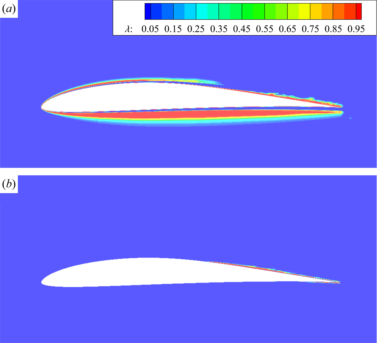
 $\lambda \to {0}$ (unconstrained far-wall region). It should be mentioned, however, that the parameterizations (2.19) and (2.20) may yield unreasonable constraint areas in laminar boundary layer as displayed in figure 1(a) for flow past the E387 airfoil, which is selected as the preliminary validation case in § 3.1. To eliminate such unphysical errors,
 $\mu _t/\mu$ is employed to distinguish the laminar regions from turbulent ones. In practice,
 $\lambda$ is slightly modified as
 \begin{equation} \lambda = \frac{1+ {\rm sign}\left(1.0, \mu_t/\mu - C_1 \right)}{2.0}\tanh \left[ {{{\left( {C_s {r_d}} \right)}^{3.0}}} \right], \end{equation}
where  $C_1$ is an empirical constant. The turbulence viscosity is usually lower than molecular viscosity for flows with low turbulence intensity. Therefore,
 $C_1$ is set to 1.0 so that
 $\lambda$ is equal to 0.0 in laminar regions of the flow. The coefficient
 $C_s$ can be modified to adjust the extent of the overlap (or constrained) area between RANS and LES regions. The larger the value of
 $C_s$, the wider the overlap region becomes. As discussed below,
 $C_s$ is always set to 8.0 in the present study. The contours of this refined control parameter are depicted in figure 1(b). As can be clearly seen, the new control parameter almost approaches 1 on the upper surface of the airfoil near the trailing edge, where a turbulent boundary is formed after laminar separation. It ought to be stressed that the successful recognition of physically correct constraint regions based on
 $\lambda$ greatly relies on the Reynolds stress model as the constraint. In other words, the turbulence viscosity
 $\mu _t$ should be able to reflect the laminar and turbulent regions of the flow.


In order for the RANS method to capture the transition phenomenon accurately, Menter et al. (Reference Menter, Smirnov, Liu and Avancha2015) propose a one-equation  $\gamma$ model for the intermittency factor:
 \begin{equation} \frac{\partial\langle\rho\rangle \gamma}{\partial t}+ \frac{\partial}{\partial x_{j}}\left(\langle\rho\rangle\left\{u_{j}\right\} \gamma\right)= P_{\gamma}-E_{\gamma} +\frac{\partial}{\partial x_{j}}\left[\left(\mu_{L}+ \frac{\mu_{T}}{\sigma_{\gamma}}\right) \frac{\partial \gamma}{\partial x_{j}}\right], \end{equation}
where  $P_{\gamma }$ and
 $E_{\gamma }$ are the production term and destruction term, respectively, which take the following forms:
 \begin{equation} P_{\gamma}=F_{length}\langle\rho\rangle\{S\} \gamma(1-\gamma) F_{onset} \end{equation}
and
 \begin{equation} E_{\gamma}=C_{a 2}\langle\rho\rangle\{\varOmega\} \gamma F_{turb}\left(C_{e 2} \gamma -1\right). \end{equation}
Here,  $\{S\}$ is the magnitude of the Favre-averaged strain rate tensor and
 $\{\varOmega \}$ is the magnitude of the Favre-averaged rotation rate tensor. For numerical prediction of transitional flows, even with a complex geometric shape, this model contains local correlations based on experimental calibration, and only requires local physical quantities. In comparison with the two-equation
 $\gamma$–
 $\widetilde {Re}_{\theta t}$ model (Menter et al. Reference Menter, Langtry, Likki, Suzen, Huang and Volker2004), the
 $\gamma$ model satisfies Galilean invariance is of much lower computational cost.
The intermittency factor  $\gamma$ is designed to approach zero in the laminar boundary layer and be close to one in the turbulent region through activating the production term when the local transition onset criterion is met. The boundary condition for
 $\gamma$ is one at inlet and zero normal flux at a wall.
The  $\gamma$ model is combined with Menter's
 $k$–
 $\omega$ SST model (Menter Reference Menter1994) by modifying the transport equations for TKE
 $k$ and specific dissipation rate
 $\omega$, which read
 \begin{gather} \frac{\partial\langle\rho\rangle k}{\partial t}+ \frac{\partial}{\partial x_{j}}\left(\langle\rho\rangle\left\{u_{j}\right\}k\right) = \gamma { P_k} + P_k^{lim} - \max (\gamma, 0.1){{ D}_k} +\frac{\partial}{\partial x_{j}} \left[\left(\mu+\sigma_{k} \mu_{t}\right) \frac{\partial k}{\partial x_{j}}\right], \end{gather}
 \begin{gather}\frac{\partial\langle\rho\rangle \omega}{\partial t} +\frac{\partial}{\partial x_{j}}\left(\langle\rho\rangle\left\{u_{j}\right\} \omega\right) =\frac{C_{\omega}\langle\rho\rangle}{\mu_{T}}{P_k} -\beta\langle\rho\rangle \omega^{2}+C{d_\omega} + \frac{\partial}{\partial x_{j}}\left[\left(\mu_{L}+\sigma_{\omega} \mu_{T}\right) \frac{\partial \omega}{\partial x_{j}}\right] . \end{gather}
The resultant RANS transition model is termed the  $k$–
 $\omega$ SST–
 $\gamma$ model (hereafter referred to as the SST–
 $\gamma$ model). Here,
 $P_k$,
 $D_k$ and
 $Cd_\omega$ are the terms in the original
 $k$–
 $\omega$ SST model (Menter Reference Menter1994). An additional production term
 $P_k^{lim}$ in the
 $k$ equation is introduced to guarantee the generation of TKE in the transition region with very low turbulence intensity. Parameter
 $\mu _t$ is the turbulence eddy viscosity which is calculated as
 \begin{equation} {\mu _t} = \frac{ \langle\rho\rangle {{a_1} \cdot k}}{{\max \left( {{a_1} \cdot \omega ,{F_2} \cdot S} \right)}}. \end{equation}
The modelled Reynolds stress tensor  $\tau _{i j}^{RANS}$ is constructed based on the Boussinesq assumption:
 \begin{equation} \tau_{ij}^{RANS} = 2\mu_{t}\left(\{S_{ij}\} - \frac{1}{3}\frac{\partial \{ u_k\}}{\partial x_k} \delta_{ij} \right) -\frac{2}{3}\rho k \delta_{ij}. \end{equation}
Likewise, the modelled Reynolds heat flux  $q^{RANS}_{i}$ is given through Reynolds analogy as
 \begin{equation} q_{i}^{RANS}={-}\frac{C_{p} \mu_{t}}{ Pr_t} \frac{\partial \{T\}}{\partial x_{i}}. \end{equation}
More details about the SST– $\gamma$ model and the corresponding constants (
 $F_{length}$,
 $C_{a_2}$,
 $C_{e2}$, etc.) can be found in the original articles (Menter Reference Menter1994; Menter et al. Reference Menter, Smirnov, Liu and Avancha2015).
For convenience of subsequent discussions, CLES refers to the LES method with modelled SGS stress and heat flux being constrained by Menter's full-turbulence  $k$–
 $\omega$ SST model, and TrCLES denotes that with SGS models controlled by the SST–
 $\gamma$ model.
2.3. Numerical methods
The governing equations (2.2) and turbulence model equations are numerically solved using an in-house solver, which is based on the cell-centred finite volume method and multi-block structured grid. The validity of this in-house code has been verified in several previous research works such as flow past a commercial aircraft (Chen et al. Reference Chen, Chen, Xia, Qu, Shi, Xiao, Liu, Cai, Liu and Lee2013), vortex shedding from bluff bodies (Cai & Chng Reference Cai and Chng2009), LPT cascade flows (Hu et al. Reference Hu, Zhou, Xia and Chen2018; Hu, Zhou & Chen Reference Hu, Zhou and Chen2020) and compressor rotor flow (Zhu, Luo & Liu Reference Zhu, Luo and Liu2018).
For the low-speed flow past the E387 airfoil, the inviscid convective fluxes of the governing equations are discretized using a second-order central scheme with artificial diffusivities, i.e. the so-called Jameson–Schmidt–Turkel scheme (Jameson, Schmidt & Turkel Reference Jameson, Schmidt and Turkel1981). For transonic flow past the T106C cascade, the inviscid fluxes are discretized via the Roe scheme (Roe Reference Roe1981). In order to reduce numerical dissipation in the Roe scheme, a hybrid method is employed for interface reconstruction (White et al. Reference White, Baurle, Fisher, Quinlan and Black2012), i.e. a fourth-order symmetric interpolation coupled with a dissipative flux reconstruction based on third-order monotone upstream scheme for conservation law. The viscous terms are calculated using Green's theorem. The temporal advancement of the equations is achieved using an implicit lower–upper symmetric Gauss–Seidel method with sub-iterations to improve the accuracy. In this paper, a non-dimensional time step  $0.0025 c/U$ is set for all simulation cases, where
 $c$ is the chord length of blade or airfoil and
 $U$ is velocity magnitude at far field for the E387 airfoil or at outlet for the T106C cascade. The results are obtained from statistical analyses for a period of time of at least
 $50 c/U$ when the flows reach their statistically stationary states.
3. Results and discussion
The E387 airfoil is a low-Reynolds-number airfoil which is characterized by a laminar separation bubble (LSB) over the suction surface and separation-induced transition at certain AoAs (McGhee, Walker & Millard Reference McGhee, Walker and Millard1988). Therefore, the E387 airfoil is selected in the present study for a preliminary validation of the proposed TrCLES method in external flow. The T106C is a typical linear UHL LPT cascade, which is characterized by a suction-side velocity peak at around the middle chord followed by a strong deceleration towards the trailing edge. Different flow patterns of separation bubble and transition may occur at various outlet Reynolds numbers and Mach numbers (Dorschner, Chikatamarla & Karlin Reference Dorschner, Chikatamarla and Karlin2017; Hu et al. Reference Hu, Zhou, Xia and Chen2018). Hence, the proposed TrCLES method is further applied to the investigation of flow past the T106C cascade at different input parameters. The numerical results are compared with the available experimental and numerical data. Meanwhile, the results from IDDES (Gritskevich et al. Reference Gritskevich, Garbaruk, Schütze and Menter2012) and CLES are also included to manifest the necessity for transition-predictive RANS models to be incorporated into the constrained SGS modelling.
3.1. Flow around the E387 airfoil
The flow past the E387 airfoil is simulated at a Reynolds number of  $Re=3.0\times 10^5$ based on a chord length
 $c$ and an AoA of
 $\alpha =1^{\circ }$. The numerical set-up is designed as such because of the availability of experimental data McGhee et al. (Reference McGhee, Walker and Millard1988) for comparison. The Mach number is set to 0.15 in the present compressible solver to approximate the incompressible limit of experimental measurement.
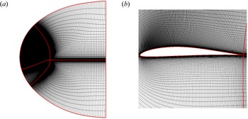
Displayed in figure 2 is a two-dimensional structured C-type grid around the E387 airfoil. The far-field boundary is located at least  $20c$ from the airfoil. The spanwise width of the computational domain is set to
 $z/c=0.2$ as a compromise between the spanwise extension and mesh resolution, which is suggested by other research groups (Sa et al. Reference Sa, Park, Kim and Park2015). According to a grid convergence study (as discussed below), the upper and lower surfaces of the airfoil contain 433 and 129 points, respectively. Furthermore, the grid contains 161 node points for the wake region in the streamwise direction, 129 in the normal direction and 65 in the spanwise direction. There are totally about 7.2 million grid cells in the simulation domain. The first off-wall grid height is about
 $5\times 10^{-5} c$, which is less than 1 in wall unit
 $y^+$.
Two-dimensional structured C-type mesh for the E387 airfoil. (a) The mesh distribution in the whole computational domain and (b) a zoom-in view around the airfoil.

The far boundary condition is implemented based on the Riemann invariants of a one-dimensional flow normal to the boundary. No-slip boundary conditions are applied to the airfoil surfaces, and the periodic boundary condition is imposed in the spanwise direction under the assumption of an infinite wing. The free-stream turbulence intensity in the present calculation is set to 0.1 % as mentioned in experiments (McGhee et al. Reference McGhee, Walker and Millard1988) and eddy viscosity ratio  $\mu _t/\mu$ is set to 0.09.
The performance of the TrCLES method can be closely related to the SGS model and transition model as the constraint. To address this issue, the Smagorinsky model is chosen as the parallel base SGS model in the TrCLES method with the model coefficient of the fluctuating part determined dynamically (detailed formulations can be found in Chen et al. (Reference Chen, Xia, Pei, Wang, Yang, Xiao and Shi2012)). The performance of the Smagorinsky model is compared with those of the helical SGS model, the corresponding TrCLES methods and the pure RANS SST– $\gamma$ model in simulations of flow past the E387 airfoil.
The pressure coefficient is an important dimensionless aerodynamic quantity defined by  $C_p = 2({p-p_\infty })/\rho _{\infty }U_{\infty }^2$. Here,
 $p$ is the local static pressure, and
 $p_\infty$,
 $\rho _{\infty }$ and
 $U_{\infty }$ are the free-stream static pressure, velocity and density, respectively, in the far field. The skin friction coefficient is another significant dimensionless aerodynamic quantity, which can be used to evaluate the correctness of predicted near-wall velocity distribution, separation and reattachment points, transition region, etc. Here, the skin friction coefficient is defined as
 $C_f=2\tau _w/\rho _{\infty }U_{\infty }^2$, where
 $\tau _w$ is the local viscous stress on the wall.
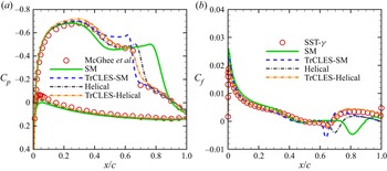
Shown in figures 3(a) and 3(b) are distributions of pressure coefficient  $C_p$ and skin friction coefficient
 $C_f$, respectively, along the surface of the E387 airfoil obtained using different methods. It is seen from figure 3(a) that the Smagorinsky model and the corresponding TrCLES method fail to predict the pressure distribution in comparison with the experimental data, especially around the separation region, though the transition constraint offered by the SST–
 $\gamma$ model exhibits a certain positive impact on the base SGS model (see the pressure recovery in the transition region). The helical model is superior to the Smagorinsky model except for the overprediction immediately after the separation bubble. The transition-constrained helical model, however, successfully improves the ability of this model. Since there are no experimental data for the skin friction coefficient, the numerical data from all other methods are compared with those from the RANS SST–
 $\gamma$ model, which are depicted in figure 3(a). As can be clearly seen, the distribution of friction coefficient given by the TrCLES-Helical model is almost identical to that calculated by the RANS SST–
 $\gamma$ model, while those provided by other methods show strong deviations from the benchmark data, especially after the separation and the induced transition regions. These results manifest that both SGS model and constraint RANS model are important in the CLES method for complex flows. While the transition model provides a necessary constraint for the transition event, the appropriate base SGS model should be employed in order to mimic the underlying flow physics. This is why the helical model is used as the base SGS model in the TrCLES method for the subsequent studies.
Distributions of (a) pressure coefficient  $C_p$ and (b) skin friction coefficient
 $C_f$ along the surface of the E387 airfoil obtained using various methods: SM, Smagorinsky model (solid); TrCLES-SM (dashed); helical SGS model, Helical (dash-dotted); TrCLES-Helical (dash-double dotted). The experimental data from McGhee et al. (Reference McGhee, Walker and Millard1988) (circles) in (a) and numerical data from the SST–
 $\gamma$ model (circles) in (b) are included for comparison.

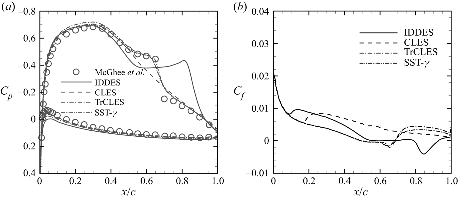
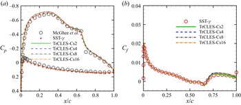
Shown in figure 4(a) are distributions of the pressure coefficients obtained by the IDDES, CLES, TrCLE and transition-predictive RANS (SST– $\gamma$ model) methods. It is clearly seen from the experimental data that the fluid over the upper surface of the airfoil accelerates first, and then decelerates. Correspondingly, the pressure (coefficient) decreases markedly from the leading edge of the airfoil, and then increases after the pressure reaches its minimum value at about one-third chord. With an increase of
 $C_p$, the boundary layer on the upper side of the E387 is subjected to adverse pressure gradient which causes separation of the boundary layer. In fact, according to the experimental data (circles) (McGhee et al. Reference McGhee, Walker and Millard1988), a LSB is formed on the upper surface in the range from about
 $0.5c$ to
 $0.7c$. In the LSB, the region where flow velocity is almost zero after the separation point is called the ‘dead air region’. The near-wall pressure coefficient in the dead air region is almost unchanged and appears as a pressure plateau. The results from both the IDDES and CLES methods show strong deviations from the experimental data in the dead air region. Although a pressure plateau can be found in the profile of
 $C_p$ predicted by the IDDES method, the width of such region is obviously overpredicted. As for the CLES method, no pressure plateau is captured at all, which indicates that the LSB is not captured, as can be seen in figure 8(b). Because the SGS models are constrained by the transition-predictive SST–
 $\gamma$ model, the TrCLES method can successfully capture the pressure distribution, which is almost identical to the experimental data and is similar to that given by the RANS simulation based on the SST–
 $\gamma$ model. Since there are no experimental data for skin friction coefficient of the E387 airfoil, the distributions of skin friction coefficient from IDDES, CLES and TrCLES are presented in comparison with that from the RANS SST–
 $\gamma$ model as shown in figure 4(b). It is clearly seen that the TrCLES method can accurately predict the separation (
 $x/c=0.5$–0.67) and the induced laminar–turbulent transition, in accordance with the performance of the SST–
 $\gamma$ model. Both IDDES and CLES fail to predict the separation and give the wrong transition points (close to the leading edge of the airfoil).
Distributions of (a) pressure coefficient  $C_p$ and (b) skin friction coefficient
 $C_f$ for the E387 airfoil at
 $Re = 3.0\times 10^5$ and
 $\alpha = 1^\circ$ obtained using various methods: IDDES (solid), CLES (dashed), TrCLES (dash-dotted) and SST–
 $\gamma$ (dash-double dotted). The experimental data (circles) given by McGhee et al. (Reference McGhee, Walker and Millard1988) are included for comparison.

The lift coefficient ( $C_L=2F_L/\rho _{\infty }U_{\infty }^2c$) and drag coefficient (
 $C_D=2F_D/\rho _{\infty }U_{\infty }^2c$) are also calculated and listed in table 1. Here,
 $F_L$ and
 $F_D$ are the total lift and drag forces, respectively. It turns out that the lift coefficients given by different methods are comparable to each other except that an obvious overshot is observed for the IDDES method. It must be mentioned that the experimental data underestimate the theory values (Eppler & Somers Reference Eppler and Somers1980) in the whole linear stage (see dashed line in figure 29 of McGhee et al. (Reference McGhee, Walker and Millard1988)). In such a sense, the SST–
 $\gamma$ model and TrCLES method offer the most reasonable results for the lift coefficient. For the drag coefficient, however, only the TrCLES method can offer a value close to the experimental measurement. This indicates that a proper description of the separation and transition processes is the key for a turbulence model to be able to accurately capture realistic flow structures and calculate aerodynamic forces.
Integral force coefficients for the E387 airfoil predicted by various methods. The experimental data (McGhee et al. Reference McGhee, Walker and Millard1988) and theoretical data (Eppler & Somers Reference Eppler and Somers1980) are included for comparison.

As mentioned above, the extent of the constrained region (between RANS and LES areas) may affect the convergence of simulation results in TrCLES, which is reflected by the value of  $C_s$ in (2.21). Here,
 $C_s$ is set to 2.0, 4.0, 8.0 and 16.0 in order to check the influence of
 $\lambda$ on the results. Shown in figures 5(a) and 5(b) are distributions of pressure coefficient
 $C_p$ and skin friction coefficient
 $C_f$ along the surface of the E387 airfoil. Overall, the results with
 $C_s=16$ show the best consistency with the experimental data and those from the SST–
 $\gamma$ model. In fact, the calculated results are not that sensitive to the control function within the present range of
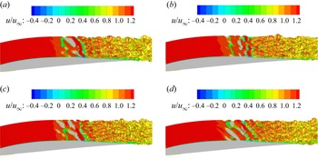
 $C_s$. In order to see how the flow structures are altered when the constant
 $C_s$ varies, we plot the isosurfaces of swirl strength, which is defined as the imaginary part of the complex eigenvalues of velocity gradient tensor and is denoted by
 $\lambda _{C_i}$. Shown in figure 6 are instantaneous flow structures around the E387 airfoil visualized by isosurfaces of
 $\lambda _{C_i}=6$ (calculated using dimensionless velocity gradient) for different
 $C_s$. It should be mentioned that the flow patterns given by the swirl strength are almost the same as those depicted by the second invariant of velocity gradient (not shown here). Some subtle local differences can be observed from these isosurfaces, especially in the separation and transition regions. In other words, changes in the size of the constraint region within a certain range have little impact on the transition and vortex developments, especially when
 $C_s$ is around 8.0. The same conclusion can be drawn from observations of the results for other values of
 $\lambda _{C_i}$. Therefore,
 $C_s$ is set to 8.0 in the subsequent simulations.
Distributions of (a) pressure coefficient  $C_p$ and (b) skin friction coefficient
 $C_f$ along the surface of the E387 airfoil at
 $Re = 3.0\times 10^5$ and
 $\alpha = 1^\circ$ obtained using different constraint areas:
 $C_s=2.0$ (solid),
 $C_s=4.0$ (dashed),
 $C_s=8.0$ (dash-dotted) and
 $C_s=16.0$ (dash-double dotted). The experimental data (circles) given by McGhee et al. (Reference McGhee, Walker and Millard1988) and numerical data from the SST–
 $\gamma$ model (plus signs and circles) are included for comparison.

Instantaneous flow structures around the E387 airfoil visualized by isosurfaces of the swirl strength ( $\lambda _{C_i}=6$) and coloured by the streamwise velocity for different constraint areas: (a)
 $C_s=2.0$, (b)
 $C_s=4.0$, (c)
 $C_s=8.0$ and (d)
 $C_s=16.0$.

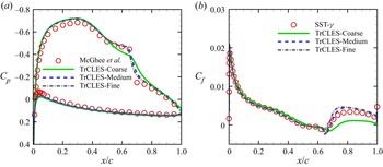
The grid convergence characteristics are of particular importance for a turbulence model, especially for practical applications. The grid convergence trend of the TrCLES method is carefully studied in the present work. Without loss of generality, the results from simulations of flow past the E387 airfoil are exhibited here to demonstrate the good grid convergence property of the TrCLES method. To this end, three sets of grids are generated with cell numbers in the circumferential and normal directions successively refined and the cell number in the spanwise direction unchanged. The grid distributions and mesh resolutions of these three sets of grids are listed in table 2, where  $N_{suction}$ and
 $N_{pressure}$ denote the numbers of circumferential node points on the suction and pressure sides of the airfoil, respectively, and
 $N_{normal}$ and
 $N_{span}$ represent the numbers of node points in the normal and spanwise directions, respectively. Shown in figures 7(a) and 7(b) are distributions of pressure coefficient
 $C_p$ and skin friction coefficient
 $C_f$ along the surface of the E387 airfoil. As can be seen, the results based on coarse grid deviate strongly from the experimental data, while those calculated based on medium and fine grids are almost identical to each other and are consistent with the experimental and reference data given by the SST–
 $\gamma$ model. This indicates that the TrCLES method has a very good grid convergence property. The conclusion also applies to the case of T106C cascade. In order to save computational resources, all other results (for both E387 airfoil and T106C cascade) presented in this paper are obtained from simulations on grids with medium resolutions.
Grid distributions and mesh resolutions for a grid convergence study of the E387 airfoil.

Distributions of (a) pressure coefficient  $C_p$ and (b) skin friction coefficient
 $C_f$ along the surface of the E387 airfoil at
 $Re = 3.0\times 10^5$ and
 $\alpha = 1^\circ$ obtained from the TrCLES method on grids with different resolutions: coarse (solid), medium (dashed) and fine (dash-dotted). The experimental data given by McGhee et al. (Reference McGhee, Walker and Millard1988) and numerical data from the SST–
 $\gamma$ model are included for comparison.

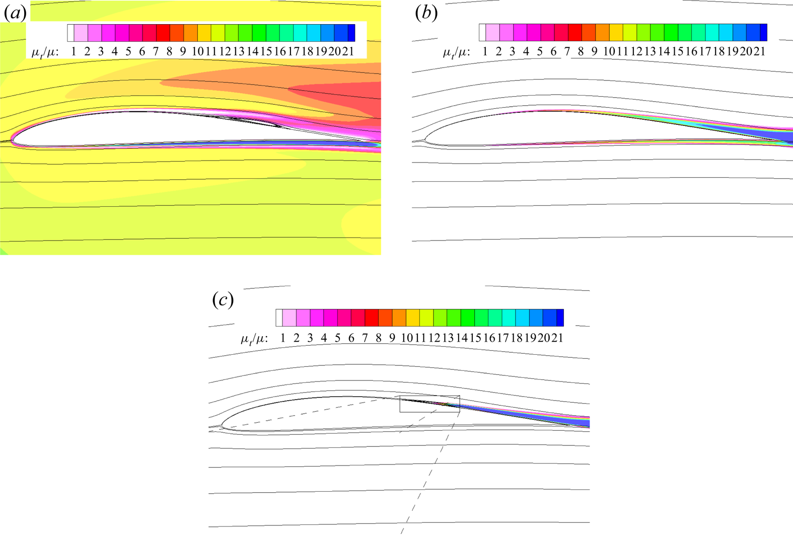
Time-averaged streamlines overlaid on contours of normalized turbulence viscosity ratio  $\mu _t/\mu$ obtained using (a) IDDES, (b) CLES and (c) TrCLES for the E387 airfoil at
 $Re = 3.0\times 10^5$ and
 $\alpha = 1^\circ$.

For both the IDDES and CLES methods, the Reynolds stress in the near-wall region is modelled based on the Boussinesq hypothesis according to (2.27). Therefore, the modelled Reynolds stresses in the boundary layer tend to vanish if turbulence eddy viscosity approaches zero. Depicted in figure 8 are time-averaged streamlines superposed on contours of normalized turbulence viscosity ratio  $\mu _t/\mu$ around the E387 airfoil obtained using different methods. As can be seen, the eddy viscosity ratio calculated by the IDDES method exhibits anomalous values even in regions far away from the airfoil, which is due to the extreme sensitivity of the model to the grid property. For the CLES method, in which the full-turbulence
 $k$–
 $\omega$ SST model is employed as the constraint, non-zero turbulence viscosities are observed in the laminar region of the flow, and no LSB is predicted as seen in experiment. The TrCLES method, with the aid of the transition-predictive
 $\gamma$ model, retains zero Reynolds stress in the laminar boundary layer and can successfully capture the transition process.
The second invariant of velocity gradient tensor is always employed to visualize flow structures (pseudo vortex structures). Formally, the second invariant of velocity gradient tensor can be given by  $Q=(\omega _i\omega _i-2S_{ij}S_{ij})/4$ with
 $\omega _i$ being the vorticity vector. Depicted in figure 9 are instantaneous isosurfaces of
 $Q$ around the E387 airfoil coloured by streamwise velocity from different methods. Due to the large separation bubble predicted by the IDDES method, three-dimensional flow structures do not appear until around the trailing edge of the airfoil. Although two-dimensional vortex structures are observed in figure 9(b), they are apparently unphysical due to incorrect Reynolds stress provided by the full-turbulence model. By contrast, the whole separation-induced transition process is accurately captured by the TrCLES method as seen in figure 9(c). Small three-dimensional flow structures are formed following the region of quasi-two-dimensional vortex structures after the reattachment point.
Instantaneous flow structures around the E387 airfoil visualized by isosurfaces of the second invariant of dimensionless velocity gradient ( $Q=20$), which are coloured by the streamwise velocity: (a) IDDES, (b) CLES and (c) TrCLES.

3.2. Transonic flow past the T106C cascade
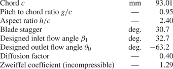
Experimental measurements on flow past the T106C cascade have been widely conducted in the framework of the European project TATMo at the von Kármán Institute for Fluid (Michálek, Monaldi & Arts Reference Michálek, Monaldi and Arts2012). The main geometric and inlet flow parameters for the T106C cascade are summarized in table 3. According to a previous suggestion (Garai et al. Reference Garai, Diosady, Murman and Madavan2016), the inlet flow angle is set to  $34.7^{\circ }$ in the present simulations in order for the pressure distributions at the leading edge of the blade to be more consistent with experimental data. The exit Reynolds number
 $Re_{2is}$ is defined based on the exit isentropic density
 $\rho _{2,is}$ and velocity
 $u_{2,is}$ as
 \begin{equation} Re_{2,is} = \frac{\rho_{2,is} u_{2,is} c}{\mu}. \end{equation}
The Reynolds number in the present study ranges from  $8\times 10^4$ to
 $2.5\times 10^5$. The isentropic Mach number can provide a measure of the local pressure and is defined as
 \begin{equation} Ma_{is} = \left[\frac{2}{\varGamma -1}\left(\left(\frac{p_{01}}{p}\right)^{{\varGamma -1}/{\varGamma}}-1 \right)\right]^{1/2}, \end{equation}
where  $p$ is local pressure,
 $p_{01}$ is inlet total pressure and the ratio of specific heats
 $\varGamma$ is set to 1.4. The exit isentropic Mach number in aforementioned experiments and the present study is 0.65.
Geometric and inlet flow parameters for the T106C cascade.

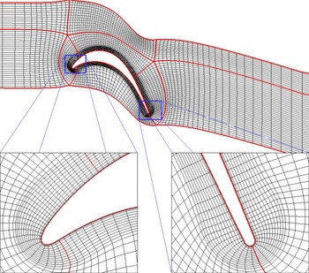
Displayed in figure 10 are the computational domain and multi-block structured grid for the T106C cascade. The inlet is located at an axial distance of  $0.95c_x$ upstream of the leading edge and the outlet is at about
 $2.5c_x$ downstream of the trailing edge. The spanwise width of the domain is set to
 $0.2c_x$. Here,
 $c_x$ is the axial chord length of the T106C cascade. This computational domain size is similar to those in previous investigations (Hillewaert et al. Reference Hillewaert, Carton de Wiart, Verheylewegen and Arts2014; Garai et al. Reference Garai, Diosady, Murman and Madavan2016). The pressure loss and outlet flow angle are directly extracted at the location of
 $0.45 C_x$ downstream of the trailing edge. Such a domain consists of only one passage in order to reduce the otherwise huge computational cost. The suction and pressure sides of the blade contain 526 and 244 cells, respectively, while 65 points are uniformly distributed in the spanwise direction. There are totally over
 $9.0 \times 10^{6}$ grid cells with a refined mesh near the wall. The first off-wall grid height is about
 $5\times 10^{-5} c$, which is less than 1 in wall units as suggested for traditional LES of wall-bounded flows. Periodic boundary conditions are imposed in the pitchwise and spanwise directions. The total pressure, temperature and flow angle are prescribed at the inlet and a static pressure condition is applied to the outlet. No-slip adiabatic wall condition is specified on the blade surface.
Two-dimensional structured grid in the whole computational domain for the T106C cascade and local zoom-in views at the leading and trailing edges. Only one out of five grid points are shown in order not to obscure the views.

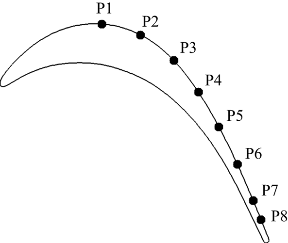
In order to observe the transition process and the corresponding characteristics of pressure fluctuations, eight numerical ‘probes’ for pressure measurement are preset on the suction side of the T106C cascade. The locations of the probes are plotted in figure 11, and their curvilinear coordinates are listed in table 4 based on the curvilinear distance on the suction surface from the leading edge.
Distributions of the ‘numerical probes’ along the suction surface of T106C.

Locations of the ‘numerical probes’ along the suction surface of T106C. Here,  $s$ is the curvilinear distance on the suction surface from the leading edge and
 $s_0$ is the curvilinear length between the leading and trailing edges.

3.2.1. Sensitivity to constraint model
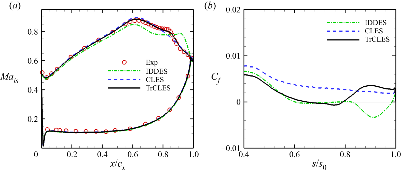
Temporally and spatially averaged physical quantities can be used to evaluate the performance of the proposed TrCLES method in prediction of T106C cascade flow. Shown in figures 12(a) and 12(b) are the distributions of time-averaged isentropic Mach number ( $Ma_{is}$) around the cascade and skin friction coefficient (
 $C_f$) along the suction side of T106C, respectively. As is clearly seen from figure 12(a), the profile of isentropic Mach number predicted by the TrCLES method is almost identical to the experimental data. The isentropic Mach number calculated by the IDDES method shows strong deviation from the experimental data, especially near the plateau region. In fact, the IDDES method significantly overpredicts the width of the pressure plateau, which corresponds to a larger and delayed separation bubble (
 $C_f<0$) as can be observed in figure 12(b). For the CLES method, however, no plateau is captured in the pressure recovery area at the suction side of the blade. This indicates that the separation bubble cannot be successfully captured by the CLES method due to the constraint of the full-turbulence SST model.
Distributions of time-averaged (a) isentropic Mach number around T106C and (b) skin friction coefficient along the suction surface of T106C at  $Re_{2,is} = 2.5\times 10^5$ obtained using different methods: TrCLES (solid), CLES (dashed) and IDDES (dash-dotted). The experimental data from Michálek et al. (Reference Michálek, Monaldi and Arts2012) (red circles) are included for comparison.

The flow over the suction side of the T106C blade starts from a laminar state, and then separates at about  $0.75c_x$. After that, transition occurs when the disturbances are amplified in the shear layer, and the flow finally turns into turbulent state. As mentioned previously, the turbulence eddy viscosity provided by the RANS model plays a key role for the correct prediction of the boundary layer flow. In laminar flow region (
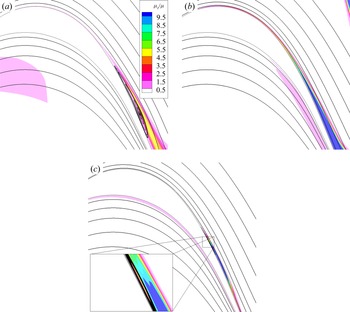
 $x/c_x<0.75$), the turbulence viscosity should be sufficiently small, and otherwise the wrong Reynolds stresses may have an irreducible impact on the mean flow. Displayed in figure 13 are time-averaged streamlines superposed on contours of normalized turbulence viscosity
 $\mu _t/\mu$ obtained using different methods. The turbulence eddy viscosity with the same order of magnitude as the laminar (molecular) viscosity can be seen in the entire boundary layer on the suction side of the blade when the full-turbulence SST model is employed (see figure 13a,b). The larger eddy viscosity ratio in the laminar boundary layer even restrains the flow separation in the CLES method as seen from figure 12(b). In contrast, the smaller eddy viscosity ratio achieved by the IDDES method cannot suppress flow separation, leading to a much larger separation bubble. The turbulence viscosity is close to zero at the laminar boundary for the TrCLES method, and rapidly increases when separation occurs as can be seen in figure 13(c). Such larger turbulence viscosity effectively restrains the formation of a large separation bubble and enhances the flow reattachment.
Time-averaged streamlines overlaid on contours of normalized turbulence viscosity  $\mu _t/\mu$ calculated using (a) IDDES method, (b) CLES method and (c) TrCLES method.

The temporal evolutions of pressure fluctuations ( $p_i^\prime =p_i-p_{i,mean}$) at different probe locations on the T106C suction surface are plotted in figure 14. Note that all the curves are modified by adding the corresponding normalized curvilinear distances from the leading edge in order to discriminate one from another. The IDDES method obtains the largest pressure fluctuations in amplitude at probes P
 $_7$ and P
 $_8$ due to the larger separation bubble. Such much larger flow structures encourage the formation of pressure disturbance waves, which travel upstream and cause large pressure fluctuations in the laminar boundary layer (see the curves at P
 $_1$–P
 $_5$ in figure 14a). For the CLES method, the amplitude of pressure disturbances increases at about the third probe (around
 $s/s_0=0.5$) as can be seen in figure 14(b), and then the flow rapidly develops into turbulent state. Compared with laminar flow, the turbulent boundary layer can resist much larger inverse pressure gradient and maintains an attached-flow regime. This is why no separation is observed in figure 13(b). As for the transition-predictive TrCLES method, the pressure fluctuations remain negligibly small in laminar attached region (
 $s/s_0 \le 0.65$), and then gradually increase after laminar separation (
 $s/s_0=0.8$).
Local normalized pressure fluctuations with respect to dimensionless time at various ‘probe’ locations of T106C calculated using (a) IDDES, (b) CLES and (c) TrCLES methods. Different curves are distinguished from each other by adding the corresponding normalized curvilinear distance from the leading edge to the normalized pressure fluctuations. Time  $t$ is non-dimensionalized using the chord
 $c$ and exit isentropic velocity
 $u_{2,is}$.

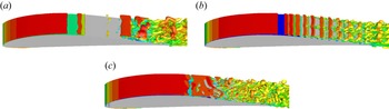
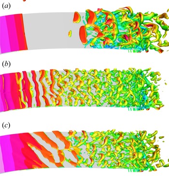
Shown in figure 15 are instantaneous isosurfaces of the second invariant of velocity gradient tensor ( $Q$) on the T106C suction surface obtained using IDDES (figure 15a), CLES (figure 15b) and TrCLES (figure 15c). For IDDES, the large flow structures appear in a very small region near the trailing edge. For CLES, unphysical near-wall flow structures are formed within a large region of the blade surface after the local pressure reaches its minimum value, which confirms again that the traditional SST model cannot provide the correct Reynolds stress in laminar boundary layer region. By contrast, much smaller flow structures are observed in TrCLES after the quasi-two-dimensional region. The well-resolved flow structures in TrCLES benefit from the facts that LES is implemented in the entire computational domain, and the laminar to turbulent transition is appropriately monitored by the SST–
 $\gamma$ model.
Instantaneous isosurfaces of the second invariant of dimensionless velocity gradient tensor ( $Q$) over the suction surface near the trailing edge of T106C obtained using (a) IDDES, (b) CLES and (c) TrCLES methods.

3.2.2. Effect of Reynolds number
For modern aircraft, a LPT usually works at Reynolds numbers ranging from  $0.5\times 10^5$ (cruise state at high altitude) to
 $5\times 10^5$ (take-off and landing states at sea level) (Hodson & Howell Reference Hodson and Howell2005). Most RANS transition models can capture the transition process accurately at high Reynolds numbers, yet they fail to predict well the transition phenomenon at low Reynolds numbers, especially for
 $Re < 1.0\times 10^5$ (Wang et al. Reference Wang, Cui and Xiao2021). Therefore, it is necessary to evaluate the performance of the proposed TrCLES method in a wider range of Reynolds numbers.
Shown in figure 16 are distributions of time-averaged isentropic Mach number around the T106C blade surface at three Reynolds numbers:  $Re_{2,is}=0.8\times 10^5$,
 $Re_{2,is}=1.2\times 10^5$ and
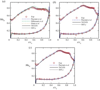
 $Re_{2,is}=1.6\times 10^5$. Both the experimental data from Michálek et al. (Reference Michálek, Monaldi and Arts2012) (red circles) and numerical data from Pacciani et al. (Reference Pacciani, Marconcini, Fadai-Ghotbi, Lardeau and Leschziner2011) (dash-double dotted) based on their own RANS transition-predictive model are included in figure 16 for comparison. The results obtained in the present RANS simulations using SST–
 $\gamma$ are also presented. Laminar separation occurs on the suction side of the blade, which is characterized by the appearance of a plateau (during the deceleration stage) on the isentropic Mach number profiles for all cases. It can be seen that the TrCLES method can predict the isentropic Mach number distributions better than RANS simulations by Pacciani et al. (Reference Pacciani, Marconcini, Fadai-Ghotbi, Lardeau and Leschziner2011), especially on the pressure side for all Reynolds numbers. Compared with RANS simulation based on the SST–
 $\gamma$ model, the TrCLES method provides a better prediction in the pressure recovery region after the pressure plateau, which can be clearly seen in figure 16(a) for the case of low Reynolds number.
Distributions of time-averaged isentropic Mach number around the T106C cascade at different Reynolds numbers: (a)  $Re_{2,is} = 0.8\times 10^5$, (b)
 $Re_{2,is} = 1.2\times 10^5$ and (c)
 $Re_{2,is} = 1.6\times 10^5$. The experimental data (red circles) are from Michálek et al. (Reference Michálek, Monaldi and Arts2012). The numerical data from Pacciani et al. (Reference Pacciani, Marconcini, Fadai-Ghotbi, Lardeau and Leschziner2011) (dash-double dotted), Hillewaert et al. (Reference Hillewaert, Carton de Wiart, Verheylewegen and Arts2014) (dash-dotted) and Garai et al. (Reference Garai, Diosady, Murman and Madavan2016) (dashed) and those given by CLES (dotted) are also included for comparison.

At  $Re_{2,is} = 0.8\times 10^5$, the numerical data from Hillewaert et al. (Reference Hillewaert, Carton de Wiart, Verheylewegen and Arts2014) (dash-dotted) at an inlet flow angle of 34.7
 $^\circ$ and Garai et al. (Reference Garai, Diosady, Murman and Madavan2016) (dashed) at an inlet flow angle of 32.7
 $^\circ$ are also displayed in figure 16(a). Both of these numerical results are obtained based on high-order discontinuous Galerkin method without the aid of extra SGS models. Hillewaert et al. (Reference Hillewaert, Carton de Wiart, Verheylewegen and Arts2014) suggest that increasing the inlet flow angle from 32.7
 $^\circ$ to 34.7
 $^\circ$ can help improve the prediction accuracy for isentropic Mach number distributions in the acceleration region on the suction side. The underestimation of isentropic Mach number within the region
 $0 \le x/c_x \le 0.4$ can be noticed from the result of Garai et al. (Reference Garai, Diosady, Murman and Madavan2016) (dashed), which is believed to be exactly due to the setting of inlet flow angle. However, changing the inlet flow angle within a small range cannot reduce the peak of isentropic Mach number (at
 $x/c_x \approx 0.6$), which is overpredicted in all simulations by Hillewaert et al. (Reference Hillewaert, Carton de Wiart, Verheylewegen and Arts2014). Garai et al. (Reference Garai, Diosady, Murman and Madavan2016) argue that this mismatch may be due to the improper set-up of inlet and outlet boundary conditions. However, in the present simulations, the peak of isentropic Mach number is bounded the employed RANS models. Due to the constraint of the transition-predictive RANS model, the TrCLES method can predict the surface loadings accurately.
As is seen in figure 16, the pure RANS computation with the  $\gamma$ transition model tends to give results almost as good as those of the proposed TrCLES method, especially as far as the statistical quantities are concerned. In fact, it is expected that the proposed TrCLES method can at least recover the results given by the pure RANS
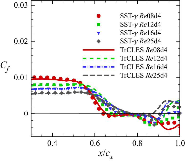
 $\gamma$ transition model because the laminar separation and transition processes are important for the development of turbulent flow and the resultant aerodynamic forces. Moreover, it is anticipated that the TrCLES method can simulate unsteady resolved fluctuations (see figure 15c) other than the LSB and the induced transition event, which is worth the increased computational cost as a whole, especially when the detailed flow structures are desired. The skin friction coefficient for the T106C cascade is further calculated at several Reynolds numbers using these two methods, which are compared with each other in figure 17. As can be seen, the length of the separation bubble is reduced with an increase of Reynolds number and the turbulent flow after transition becomes reattached when approaching the trailing edge of the cascade. It is clear that the friction coefficient calculated by TrCLES method almost collapses onto that given by the SST–
 $\gamma$ model before the separation point, but the former predicts a smaller separation bubble in comparison with the SST–
 $\gamma$ model, which is attributed to the unsteady effect of fluctuating structures captured by the TrCLES method.
Distributions of time-averaged skin friction coefficient  $C_f$ along the suction surface of T106C cascade obtained from SST-
 $\gamma$ model and TrCLES method at different Reynolds numbers:
 $Re_{2,is} = 0.8\times 10^5$ (solid line and circles),
 $Re_{2,is} = 1.2\times 10^5$ (dashed line and squares),
 $Re_{2,is} = 1.6\times 10^5$ (dash-dotted line and down triangles) and
 $Re_{2,is} = 2.5\times 10^5$ (long-dashed line and diamonds).

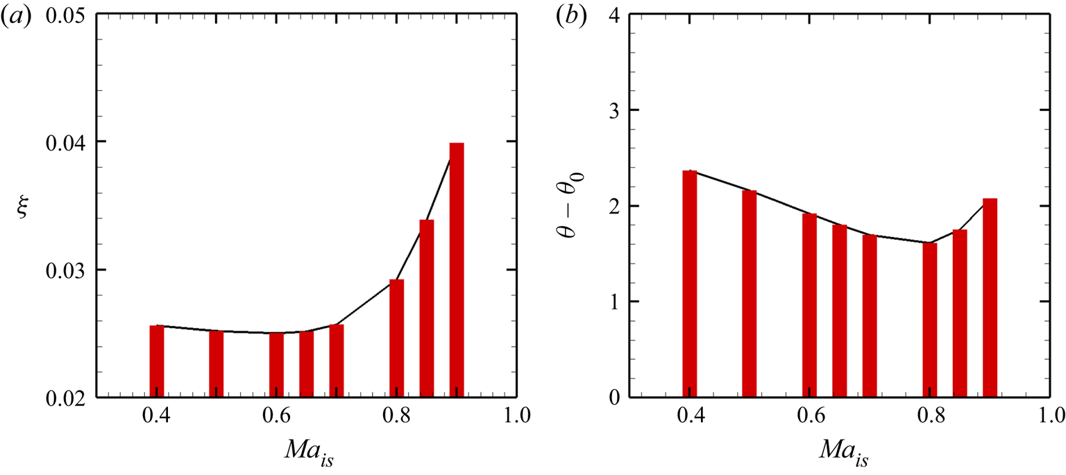
The kinetic energy loss and outlet flow angle are important quantities for the aerodynamic performance of a LPT. The kinetic energy loss coefficient is defined as
 \begin{equation} \xi = 1 - \left[ {1 - {{\left( \frac{\overline{p}_{2} }{\overline{p}_{02} } \right)}^{{{\varGamma - 1}}/{\varGamma}}}} \right]/\left[ {1 - {{\left( {\frac{{\overline{p}_{2} }}{\overline{p}_{01} }} \right)}^{{{\varGamma - 1}}/{\varGamma }}}} \right]. \end{equation}
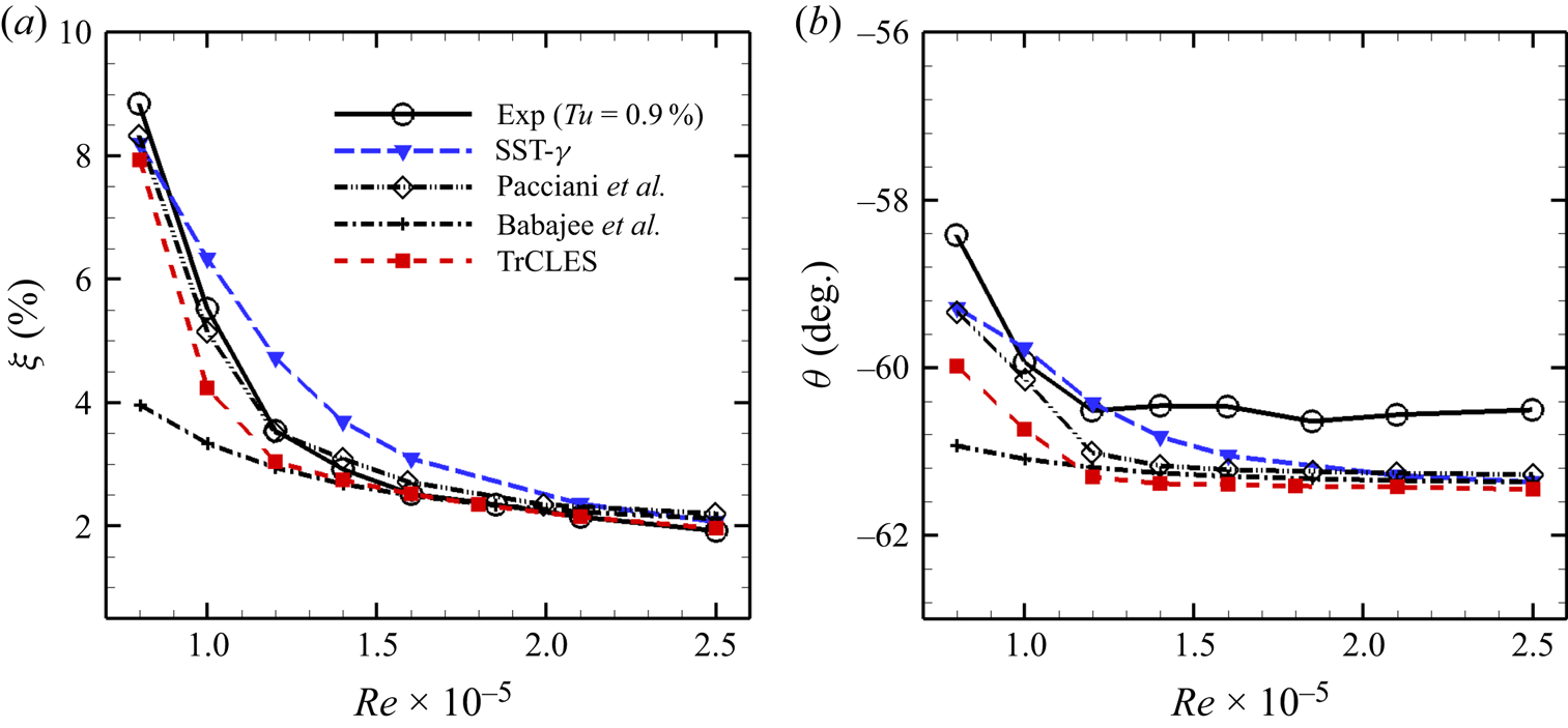
The mass-averaged kinetic energy loss coefficient and exit flow angle at  $x/c_x=1.45$ downstream of the leading edge of T106C are compared with the experimental data given by Michálek et al. (Reference Michálek, Monaldi and Arts2012) in figures 18(a) and 18(b), respectively. The numerical data from Pacciani et al. (Reference Pacciani, Marconcini, Fadai-Ghotbi, Lardeau and Leschziner2011), Babajee & Arts (Reference Babajee and Arts2012) and the present RANS simulations based on the SST–
 $\gamma$ model are also included for comparison. As can be seen, the best comparisons are those of Pacciani et al. (Reference Pacciani, Marconcini, Fadai-Ghotbi, Lardeau and Leschziner2011), who employ a transition model based on a laminar kinetic energy concept. Both the kinetic energy loss coefficient and exit flow angle are seriously underestimated at low Reynolds numbers in the RANS simulation of Babajee & Arts (Reference Babajee and Arts2012), who employ the correlation-based two-equation transition model proposed by Langtry & Menter (Reference Langtry and Menter2009). In comparison with the SST–
 $\gamma$ RANS transition model, a better agreement is achieved between the numerical results predicted by the TrCLES method and the experimental data for exit mass-averaged kinetic energy loss coefficient. As for the exit flow angle, the values provided by all the numerical methods show large deviations from the experimental results, especially for high-Reynolds-number cases (about
 $1^{\circ }$ difference).
(a) Mass-averaged kinetic energy loss coefficient and (b) exit flow angle with respect to Reynolds number at  $x/c_x=1.45$ downstream of the leading edge of the T106C cascade. The experimental data from Michálek et al. (Reference Michálek, Monaldi and Arts2012) (solid line with open circles) and the numerical data from Pacciani et al. (Reference Pacciani, Marconcini, Fadai-Ghotbi, Lardeau and Leschziner2011) (dash-double dotted line with open diamonds), Babajee & Arts (Reference Babajee and Arts2012) (dash-dotted line with plus signs) and the present CLES (dashed line with solid down triangles) are included for comparison.

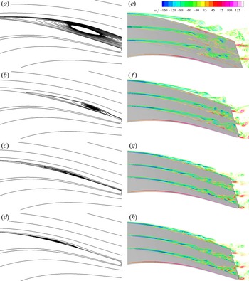
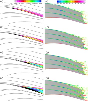
Depicted in figure 19 are time-averaged streamlines and contours of instantaneous spanwise vorticity in the separation region on the suction side of T106C for Reynolds number ranging from  $0.8\times 10^5$ to
 $1.4\times 10^5$. As illustrated by the streamlines, the pattern of separation bubble is transformed from an ‘open bubble’ mode (without reattachment on the blade suction side) (
 $Re_{2,is} =0.8\times 10^5$) to a ‘long bubble’ mode (
 $Re_{2,is} = 1.4\times 10^5$). The smaller the LSB, the narrower the pressure plateau, as seen in figure 16. Upstream of the separation bubble, the shear layer with negative spanwise vorticity attaches to the suction surface in the laminar boundary layer, and then departs from the blade to form a free shear layer due to inverse pressure gradient, which breaks into small vortices with the growth of disturbances. When
 $Re_{2,is} =0.8\times 10^5$, the shear layer exhibits a large departure from the wall in the laminar separation zone, which greatly intensifies flow mixing with a tremendous augmentation in energy loss (see figure 18a) and a high under-turning in exit flow angle (see figure 18b). Although laminar separation still occurs at
 $Re_{2,is} = 1.4\times 10^5$, the shear layer is lifted up only a small distance from the wall. After transition, the flow reattaches to the surface again prior to the trailing edge, which leads to a modest rise of the energy loss and a limited impact on the exit flow turning.
(a–d) Time-averaged streamlines and (e–h) contours of instantaneous spanwise vorticity in three  $x$–
 $y$ plane slices over the suction side of T106C obtained using the TrCLES method at various Reynolds numbers: (a,e)
 $Re_{2,is} = 0.8\times 10^5$, (b,f)
 $Re_{2,is} = 1.0\times 10^5$, (c,g)
 $Re_{2,is} = 1.2\times 10^5$ and (d,h)
 $Re_{2,is} = 1.4\times 10^5$.

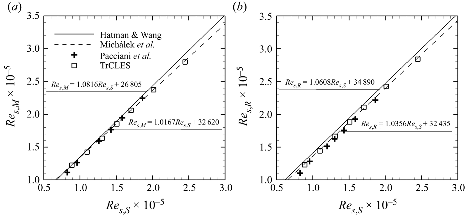
Some characteristic points such as the separation point, reattachment point and maximum bubble elevation point are important indicators for examining the correctness of predicted location and size of a separation bubble and gaining insight into the physical aspects of the bubble structures. As suggested by Hatman & Wang (Reference Hatman and Wang1999), a local (or distance) Reynolds number can be used to express the positions of these characteristic points, which is defined as  $Re_{s}={s V_{\infty,s}}/{\nu _s}$ with
 $s$ being the curvilinear distance from the leading edge of the airfoil,
 $V_{\infty,s}$ the mean inlet velocity and
 $\nu _s=\mu _s/\rho _s$ the local kinematic viscosity. For example, one can define the local Reynolds number at separation point
 $Re_{s,S}$, reattachment point
 $Re_{s,R}$ and maximum bubble elevation point
 $Re_{s,M}$.
Hatman & Wang (Reference Hatman and Wang1999) suggest that the experimental data for low free-stream turbulence flat plate and airfoil expressed in terms of local Reynolds number should be correlated better than momentum or displacement thickness Reynolds number. For incompressible flows with low levels of turbulence intensity ( $Tu=0.3\,\%\text {--}0.6\,\%$), Hatman & Wang (Reference Hatman and Wang1999) develop a correlation-based prediction model for separated-flow transition, which takes the following forms:
 \begin{gather} Re_{s,M} = 1.0816Re_{s,S} + 26\,805, \end{gather}
 \begin{gather}Re_{s,R} = 1.0608Re_{s,S} +34\,890. \end{gather}
Taking into account the compressibility effect of the flow, Michálek et al. (Reference Michálek, Monaldi and Arts2012) propose a modification of the above correlation model based on the experimental data of T106C cascade in the forms
 \begin{gather} Re_{s,M} = 1.0167 Re_{s,S} + 32\,620, \end{gather}
 \begin{gather}Re_{s,R} = 1.0356 Re_{s,S} +32\,435. \end{gather}
Shown in figures 20(a) and 20(b) are the Reynolds numbers for maximum bubble displacement ( $Re_{s,M}$) and reattachment location (
 $Re_{s,R}$) as a function of the local Reynolds number at separation points (
 $Re_{s,S}$), respectively, obtained using the present TrCLES and reported by Pacciani et al. (Reference Pacciani, Marconcini, Fadai-Ghotbi, Lardeau and Leschziner2011) based on the transition-predictive RANS model. The prediction models proposed by Hatman & Wang (Reference Hatman and Wang1999) and Michálek et al. (Reference Michálek, Monaldi and Arts2012) are also included for comparison. As can be seen, the variations of local Reynolds numbers at the maximum bubble thickness point and reattachment point with respect to the separation point Reynolds number all exhibit a linear behaviour, similar to that of the two prediction models.
Local Reynolds numbers at (a) maximum displacement location and (b) reattachment point as a function of the local Reynolds number at separation point obtained using the present TrCLES (open squares). The correlations provided by Hatman & Wang (Reference Hatman and Wang1999) (solid) and Michálek et al. (Reference Michálek, Monaldi and Arts2012) (dashed) and the numerical result given by Pacciani et al. (Reference Pacciani, Marconcini, Fadai-Ghotbi, Lardeau and Leschziner2011) (plus signs) are included for comparison.

In view of the formulations for the two prediction models, the correlation between maximum bubble displacement and separation points given by Michálek et al. (Reference Michálek, Monaldi and Arts2012) is a little smaller in slope and larger in intercept than that proposed by Hatman & Wang (Reference Hatman and Wang1999). Both the slope and intercept of the correlation function between reattachment and separation points are smaller in the compressible case than its incompressible counterpart. It should be mentioned again that all the experimental data used by Hatman & Wang (Reference Hatman and Wang1999) are from incompressible flows for flat plate and airfoil. However, the exit Mach number in the present simulations for T106C cascade is 0.65 and much higher Mach number can be achieved on the blade suction side. Under such condition, the impact of compressibility on the LSB cannot be ignored. Compared with data from Pacciani et al. (Reference Pacciani, Marconcini, Fadai-Ghotbi, Lardeau and Leschziner2011), the present TrCLES results are almost identical to the correlations proposed by Michálek et al. (Reference Michálek, Monaldi and Arts2012), especially at low local Reynolds numbers. These results indicate that the proposed TrCLES method can successfully capture the separation bubble behaviours and the Reynolds number effect.
3.2.3. Effect of Mach number
Mach number, which reflects the relative importance of kinetic energy to internal energy, can also be used to measure the compressibility of gas flows. Different exit Mach numbers inevitably lead to various wave and flow structures in an UHL LPT, and as a result, have significant influence on flow loss of the turbine. Three exit Mach numbers (0.6, 0.65 and 0.7) are first examined to validate the ability of the transition-predictive TrCLES method to recognize the levels of compressibility of turbine flows. Displayed in figures 21(a) and 21(b) are distributions of time-averaged isentropic Mach numbers for different exit Mach numbers obtained in the present RANS simulation based on the SST– $\gamma$ model and TrCLE, respectively, in comparison with the corresponding experimental data provided by Michálek et al. (Reference Michálek, Monaldi and Arts2012). The exit Reynolds number is
 $Re_{2,is} = 1.6\times 10^5$. With an increase of exit isentropic Mach number, the isentropic Mach number curve tends to be lifted upwards on the suction side and remains almost unchanged on the pressure side, which means that the loading of the blade is increased. The isentropic Mach number distributions obtained using transition-predictive RANS simulation and TrCLES are almost identical to the experimental data. At
 $Ma_{2,is} = 0.7$, the SST–
 $\gamma$ model cannot capture the isentropic Mach number accurately at the turning point from the pressure plateau to recovery region, which is similar to the performance at low Reynolds numbers. The TrCLES method, however, effectively improves the accuracy of prediction at this turning point though the mean modelled SGS quantities are constrained by the same SST–
 $\gamma$ model.
Distributions of time-averaged isentropic Mach number at different exit Mach numbers and exit Reynolds number  $Re_{2,is} = 1.6\times 10^5$. (a) The RANS method with the SST–
 $\gamma$ model and (b) TrCLES. The experimental data from Michálek et al. (Reference Michálek, Monaldi and Arts2012) (symbols) are included for comparison.

Furthermore, a wider range of the isentropic exit Mach numbers from 0.4 to 0.9 are considered at the same Reynolds number  $Re_{2,is} = 1.6\times 10^5$ to study the compressibility effect on the flow patterns and aerodynamic performances of T106C. Shown in figures 22(a) and 22(b) are distributions of time-averaged isentropic Mach number around the blade and skin friction coefficient on the suction side at different exit Mach numbers, respectively. With an increase of exit Mach number, the isentropic Mach number undergoes more prominent uplift on the suction side than on the pressure side. Meanwhile, the location for the peak value of
 $Ma_{is}$ tends to move downstream. Thus, much stronger adverse pressure gradient acts on the rear part of the T106C suction side, causing much larger flow separation at high exit Mach number. As one can clearly see in figure 22(b), with an increase of exit Mach number, the separation point first moves downstream for
 $Ma_{2,is} \le 0.8$, and then travels upstream again for
 $Ma_{2,is} >0.8$. The reattachment point, however, moves monotonically towards the trailing edge. This can be seen more clearly in figure 24(a–d), where the time-averaged separation bubble passes from ‘short’ mode to ‘long’ mode when pushed downstream on the blade suction side with an increase of exit Mach number.
(a) Distributions of time-averaged isentropic Mach number around the T106C cascade and (b) skin friction coefficient on the suction surface at different exit Mach numbers and  $Re_{2,is} = 1.6\times 10^5$.

Displayed in figures 23(a) and 23(b) are mass-weighted kinetic energy loss coefficient and relative exit flow angle at  $x/c_x = 0.45$ downstream of the trailing edge of T106C cascade, respectively. The exit kinetic energy loss coefficient first drops slightly with increasing
 $Ma_{2,is}$ until reaching its local minimum value near
 $Ma_{2,is} = 0.6$, and then the loss coefficient experiences a sharp growth, which is consistent with the observation by Abraham et al. (Reference Abraham, Panchal, Xue, Ekkad, Ng, Brown and Malandra2010). By contrast, the exit flow angle decreases much faster with the exit Mach number when
 $Ma_{2,is} <0.7$, and then reaches its minimum value at
 $Ma_{2,is} \approx 0.8$. Therefore, the exit flow angle is much more easily affected by the exit Mach number when
 $Ma_{2,is} \le 0.7$. In fact, the flow near the trailing edge on the suction side undergoes more rapid acceleration than that on the pressure side with an increase of exit Mach number, which leads to a decrease of the exit flow angle. Nevertheless, the kinetic energy loss is mainly caused by boundary layer mixing. The flow loss near the exit remains almost unchanged due to the small separation bubbles and thin boundary layers at low exit Mach numbers.
(a) Mass-weighted kinetic energy loss coefficient  $\xi$ and (b) relative exit flow angle
 $\theta -\theta _0$ with respect to the isentropic exit Mach number at
 $x/c_x = 0.45$ downstream of the trailing edge of T106C with
 $Re_{2,is} = 1.6\times 10^5$.

(a–d) Time-averaged streamlines overlaid on contours of resolved TKE and (e–h) contours of instantaneous spanwise vorticity in three  $x$–
 $y$ plane slices over the suction side of T106C obtained using the TrCLES method at
 $Re_{2,is} = 1.6\times 10^5$ and various isentropic exit Mach numbers: (a,e)
 $Ma_{2,is} = 0.4$, (b,f)
 $Ma_{2,is} =0.6$, (c,g)
 $Ma_{2,is} = 0.8$ and (d,h)
 $Ma_{2,is} = 0.9$. The resolved TKE
 $k_{res}$ is normalized by
 $u^2_{2,is}$.

Likewise, we show in figure 24 the time-averaged streamlines superposed on resolved TKE (figure 24a–d) and contours of instantaneous spanwise vorticity (figure 24e–h) in three  $x$–
 $y$ plane slices near the separation bubble regions of the T106C flows at various exit Mach numbers. The time-averaged separation bubble tends to move downstream and experiences a transition from ‘short’ mode to ‘long’ mode as the exit Mach number increases. Meanwhile, the shear layer after separation breaks into much more complex flow structures which manifest that the transition point successively moves downstream with increasing exit Mach number. The resolved kinetic energy emerges due to the unsteadiness of the shear layer after separation, and increases to its maximum value near the reattachment point. The peak value of resolved kinetic energy tends to be intensified with an increase in size of the separation bubble. The region of non-zero resolved kinetic energy, in which turbulent mixing takes place, is much thicker than the corresponding separation bubble.
The power spectral densities (PSDs) of pressure fluctuations at different probe points on the blade suction surface are depicted in figure 25 for four exit Mach numbers. The PSD at the monitoring point in the laminar flow region (corresponding to the regions of low resolved TKE in figure 24) is much smaller than that at the monitoring point in turbulent boundary layer (corresponding to the regions of high resolved TKE in figure 24). At point P $_5$, the transition process is almost completed when
 $Ma_{2,is} = 0.4$, while the onset of transition is just observed when
 $Ma_{2,is} = 0.6$. When the exit Mach number increases to 0.8, the boundary layer still remains laminar at P
 $_5$, and transition takes place just ahead of the monitoring point P
 $_6$. This is because the separation point and transition point move downstream when
 $Ma_{2,is} \le 0.8$. When
 $Ma_{2,is} = 0.9$, the distribution of PSD at P
 $_6$ is almost identical to that at P
 $_8$, which means that the transition is almost completed at P
 $_6$. The transition starts earlier at
 $Ma_{2,is} = 0.9$ than at
 $Ma_{2,is} = 0.8$ because the separation point turns to move upstream when the exit Mach number increases from 0.8 to 0.9 as shown in figure 24.
The PSD of the pressure fluctuations at different monitoring points for  $Re_{2,is} = 1.6\times 10^5$ and various isentropic exit Mach numbers: (a)
 $Ma_{2,is} = 0.4$, (b)
 $Ma_{2,is} =0.6$, (c)
 $Ma_{2,is} = 0.8$ and (d)
 $Ma_{2,is} = 0.9$.

The resolved Reynolds stress  $R_{uv}^{res}=-\langle \bar {\rho }\rangle (\{\tilde {u}_{i}\tilde {u}_{j}\}-\{\tilde {u}_{i}\}\{\tilde {u}_{j}\})$ in terms of distance to the nearest wall
 $d_w$ at several monitoring points is shown in figure 26 for different exit Mach numbers. At low background turbulence level, the boundary layer transition on the blade suction side usually starts from the free shear layer after separation. The free shear layer is affected by small disturbances and breaks up to develop into turbulent boundary layer. In light of the distribution of resolved Reynolds stress, the separated shear layer is located at regions of certain distances away from the wall as marked by the grey area in figures 26(c) and 26(d). When the separation bubble is large enough in a ‘long’ mode (
 $Ma_{2,is}\ge 0.8$), the disturbances (or velocity fluctuations) grow gradually in the shear layer after separation. When the exit Mach number is quite low (the separation bubble is small in a ‘short’ mode), only weak development of disturbances is observed in the shear layer as illustrated in figure 26(a,b).
Resolved Reynolds stress  $R_{uv}^{res}$ with respect to distance to the nearest wall
 $d_w$ at six successive monitoring points for
 $Re_{2,is} = 1.6\times 10^5$ and various isentropic exit Mach numbers: (a)
 $Ma_{2,is} = 0.4$, (b)
 $Ma_{2,is} =0.6$, (c)
 $Ma_{2,is} = 0.8$ and (d)
 $Ma_{2,is} = 0.9$. Each curve is plotted by adding a constant in order to distinguish one from another.

4. Conclusions
In this paper, a three-equation RANS transition model (SST– $\gamma$ model) is suggested to constrain the SGS models in the CLES method (referred to as the TrCLES method) to improve its accuracy in predicting wall-bounded laminar to turbulent transition flows. Both external (E387 airfoil) and internal (UHL LPT T106C cascade) flows are selected to verify the validity of the proposed TrCLES method for the availability of corresponding experimental data. The results are also compared with those from IDDES, CLES based on full-turbulence
 $k$–
 $\omega$ SST model and RANS simulation with transition-predictive SST–
 $\gamma$ model. It is manifested that the TrCLES method can predict laminar separation, transition process and turbulent attachment events more accurately than all other methods under consideration.
For both the E387 airfoil and T106C cascade flows, the original CLES and IDDES methods based on the full-turbulence SST model cannot accurately predict the LSB and separation-induced transition. Although the IDDES method can capture a separation bubble, it seriously overestimates the size of the time-averaged LSB, which is attributed to the small eddy viscosity offered by the IDDES method in the near-wall region close to the trailing edge. By contrast, no LSB is obtained using the original CLES method because the non-zero eddy viscosity results in non-physical Reynolds stress (and heat flux) in laminar boundary layer region. The TrCLES method, however, offers almost zero Reynolds and SGS stresses (and heat fluxes) in laminar boundary layer with the aid of the SST– $\gamma$ model and sufficient Reynolds stresses in turbulent boundary layer so that it can predict LSB structure and transition process with encouraging accuracy.
The TrCLES method is then employed to investigate the effects of isentropic exit Reynolds number and Mach number on the flow patterns, transition behaviour and aerodynamic performance of T106C cascade and further evaluate the validity of this new method. In comparison with the RANS method based on the SST– $\gamma$ model, the TrCLES method can capture the distribution of isentropic Mach number (or, equivalently, static pressure) more accurately around the turning point from the pressure plateau to recovery region at low Reynolds numbers or high exit Mach numbers. Moreover, the TrCLES method proves to be superior to the RANS method Abraham et al. (Reference Abraham, Panchal, Xue, Ekkad, Ng, Brown and Malandra2010) in prediction of the correlations between the characteristic points of the separation bubble, which are represented by local (or distance) Reynolds numbers.
In summary, the TrCLES method with the SGS models constrained by the SST– $\gamma$ model can not only accurately predict the LSB structure and time-averaged flow variables, but also perform well in prediction of the whole unsteady separation-induced transition flow of T106C cascade. It ought to be stressed that the present TrCLES method fails to calculate the exit flow angle accurately compared with the experimental results. However, it seems that the systematic error in exit flow angle is shared by all other methods. Realization of such an ability requires further study of the transition-predictive RANS model as the constraint, though such an error may not be caused by transition prediction. Calibration optimization procedure or artificial intelligence techniques based on more reliable experimental and DNS data of various geometries may help pave the way for further improvement of the present TrCLES method.
Acknowledgements
Numerical simulations were carried out on the Polaris computing platform of Peking University in Beijing and the Tianhe-2 supercomputing facility at the National Supercomputer Center in Guangzhou, China.
Funding
The authors acknowledge the financial support provided by the National Natural Science Foundation of China (grant nos. 92152202 and 11988102). This work was also supported by the National Key Project (grant no. GJXM92579).
Declaration of interests
The authors report no conflict of interest.