Introduction

Although it is known that snow redistribution by wind in high mountains is one of the most important factors inducing avalanche risk, it has been considered in physical and numerical avalanche forecasting models (Reference Föhn and HaechlerFöhn and Haechler, 1978; Reference MeisterMeister, 1989) but only recently in expert models (Reference Schweizer and Föhn.Schweizer and Föhn, 1996). This is because of the poor knowledge of the volume of snow moved and deposited by the wind. Efficient modelling of avalanche paths and snow volumes requires good knowledge of the amount of accumulated and eroded snow at the avalanche-starting zone. This is why, in 1987, the Division Nivologie of CEMAGREF decided to develop a knowledge-based system for modelling avalanche-path analysis: the ELSA (Étude des Limites de Sites Avalancheux) system (Reference Buisson and CharlierBuisson and Charlier, 1990, Reference Buisson and Charlier1993; Reference Mases, Buisson, Good and VilaplanaMases and others, 1995a, Reference Mases, Buisson, Frey and Sivardièreb). In particular the ELSA system is aimed at helping specialists in avalanche-path analysis, by giving them a complete working environment and all the necessary tools for avalanche prediction.

The ELSA system is composed of different modules which correspond to the different stages of the programme (Fig. 1): first, the programme simplifies the numerical topographic data input (digitized topography) by irregular triangulation in order to build quasi-homogeneous units of the Earth’s surface called “panels” (Fig. 2). Calculations developed by the programme are referred to the panels. Panel boundaries are ridges, thalwegs and natural wedges; secondly, the System calculates the mean snow height for each panel after a wind period (snow-wind module); and finally the system determines which panels correspond to the avalanche-starting zone and which ones are involved in the avalanche process (avalanche track and run-out zones). The ELSA system is also able to calculate the avalanche velocity and snow mass involved in the avalanche.

Fig. 1.

The expert system ELSA is composed of different modules, which help to approximate finally the avalanche velocity and snow mass in a given avalanche track.

Fig. 2.

The Still berg site: the ground surface is simplified in units called panels.

The different modules of the system work interactively. In this paper, we present the validation and improvement of the second module (snow-wind module) with real data from Stillberg, Switzerland. Field data have been analysed (Reference Mases, Buisson, Good and VilaplanaMases and others, 1995a) in order to understand the spatial distribution of the snow transported by wind in avalanche-starting zones. The results have been used to develop a new empirical model for snowdrift distribution which constitutes the model for the snow-wind module.

First, we describe how the new model takes into account the topography; then, we describe the parameters used by the model to calculate the spatial distribution of the snow and how to obtain these parameters from field data; and finally, we describe how the model uses these parameters to simulate snow distribution.

Field data come from the Stillberg site in the Dischma Valley, Switzerland, a northeast-facing slope with avalanche-starting zones at an altitude of about 2200 m a.s.l. The site was instrumented in 1958 by the Swiss Federal Institute for Snow and Avalanche Research and there are more than 30 years of continuous data records. The site is instrumented with vertical stakes, i.e. 433 poles scattered on the slope, which enabled us to study the snow-depth evolution in the avalanche-starting zone by remote observations (there are about five stakes in every panel). These snow poles provide accurate data on snow height in the accumulation and erosion zones. The site is also equipped with meteorological stations which allow us to characterize the weather conditions.

The Snow-Wind Module

The module of the ELSA system calculates the distribution of snow height in the avalanche zone after a wind period. The model takes into account all possible combinations of slopes on both sides of the ridges (leeward and windward). These are synthesized into 17 types of ridge (Fig. 3). The slope intervals depend on the critical angles. For example, an angle of 28° is considered as the minimum angle (Reference SalmSalm, 1983) and an angle of 45–50° the maximum angle to produce an avalanche.

Fig. 3.

In the snow wind module all possible combinations of ridges are synthesized as 17 types. Every kind of ridge has four types of panel: A, panel on the windward side not close to the edge; B, panel on the windward side close to the edge; C, panel on the leeward side close to the edge; D, panel on the leeward side not close to the edge (γ, windward slope angle; ϕ, leeward slope angle).

The model calculates the mean snow height in the panels, depending on their positions relative to the edges. It is considered that one panel is affected by one edge, if it is located in the influence zone according to Figure 4. According to this, slopes at the Stillberg site are divided into 68 different types of panel, according to their position:

The panels are constant during a single snowdrift period. The model only works during drifting periods which have a constant wind direction.

Fig. 4.

Drift influence zone around a ridge. A, B, C and D are in the influence zone of a ridge. A, not close to the edge on the windward side; B, close to the edge on the windward side; C, close to the edge on the leeward side; D, not close to the edge on the leeward side. E is not in a ridge-influence zone.

Calculation of the snow height for each panel is obtained from a parameter called the “wind coefficient (c)” (Reference Mases, Buisson, Frey and SivardièreMases and others, 1995b). This coefficient represents the relation between the snow accumulated (snow height) before the end of a drilling period (h₂ ) and the snow available (snow height) for transport at the beginning of a drifting period (h₁) as shown in Figure 5.

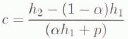
where h₁ is the snow height before a drifting period, h₂ is the snow height at the end of such a period, α is the percentage of snowpack susceptible to erosion and p is the solid precipitation.

Fig. 5.

The wind coefficient (c) represents the relation between the accumulated snow (c(αh₁ + p)) at the end of a drift period and the snow available for transport at the beginning of the wind period (αh₁). p is the solid precipitation and (1 − α)h₁ is the percentage of snowpack that cannot he eroded.

The snow—wind module does not take into account the nivo-meteorological periods with liquid precipitation.

This wind coefficient multiplied by the volume of available snow during a wind period (snow of the snowpack susceptible to be eroded (α) and snow of precipitation) gives the snow height on each panel. The wind coefficient can be established from the field data (see below). The wind periods are variable in length and according to wind speed and have a duration between 1 and 5 days. As a threshold wind speed for snow drift, a wind speed of 6 m s⁻¹ was chosen.

The use of the wind coefficient as representative of the spatial snow distribution is justified by the good correlation between snow distribution from field data (Stillberg site) for one nivo-meteorological event and the calculated wind coefficient in Figure 6. In this figure, the lefthand map represents the snow-height difference (H = h₂ − h₁) distribution at the end the snowdrifting period: 3–6 December 1964. The righthand map represents the wind-coefficient distribution at the end of the same drifting period. We can observe that the zones with erosion have a low wind-coefficient value and the zones with snow accumulation have a high wind-coefficient value.

Fig. 6.

On the lefthand side the snow-height difference distribution at the end of the drift period (3–6 December 1964) is represented. On the righthand side, the wind-coefficient distribution at the end of the same wind period is given.

Obtaining the Wind Coefficient from Field Data

The wind coefficient can be evaluated from field data. The following parameters are needed: (a) the snow height before the wind period (h₁); (b) the snow height at the end of the wind period (h₂); (c) the solid precipitation (p); (d) the percentage of snow in the snowpack susceptible to be eroded (α). In the case of the Stillberg site, h₁ and h₂ are known from measurements on the snow poles and P is known from the nivo-meteorological data. The value of α was obtained from stratigraphic snow profiles. We determine which snow layers could be eroded empirically. For example, rather fresh snow, small rounded grains or faceted crystals of low ram hardness are considered erodable but large rounded particles and ice could not be eroded (cf. Fig. 7).

Fig. 7.

In the model the α coefficient is obtained from stratigraphic snow profiles. We determine in an empirical way which are the snow layers that can be eroded. This figure shows two examples of stratigraphic snow profiles with an associated wind coefficient.

The nivo-meteorological conditions were synthesized in 20 period types (Fig. 8). For each , the wind coefficient (c) was calculated for each kind of panel. As different values of c may be obtained, because of the amount of Stillberg data, and because of other snow parameters not evaluated in this paper, the value introduced in the model is one which represents the major frequency. Finally, a list of wind coefficients for each type of nivo-meteorological scenario and for each kind of panel was obtained. This database was used by the model to determine the wind coefficient on each panel.

Fig. 8.

Synthesis of the nivo-meteorological conditions. The parameters that we have used to reach this classification are: scenario of wind period (wind episode), amount of snow precipitation and snowpack surface particles.

Application of the Model

This model can be applied to different regions. For this, it is necessary to have a digital topographic database and knowledge of the mean wind direction and speed during the period we wish to model.

The procedure is as follows. First, the topographic data are entered into the program and the panels are established. Then, the nivo-meteorological scenario, most similar to that to be simulated (represented in Figure 8), is selected. The snow wind module will automatically find the nearest edge for each panel and the relationships between that panel and the edge (i.e. leeward or windward orientation of the panel and whether it is close to the edge or not). Once the panel has been characterized spatially, the wind coefficient is assigned automatically. Multiplication of the wind coefficient by the snow available at the beginning of the wind period gives the snow height on each panel at the end of the wind period.

Figure 9 shows four maps: a′ and b′ represent the wind-coefficient distribution calculated from the field data (at Stillberg) for two nivo-meteorological periods. Maps a and b show the simulated distribution of the wind coefficient for the same two nivo-meteorological periods using this model. Map b shows a fair correspondence with map b′ (i.e. the real distribution of the wind coefficient), whereas in the case of maps a and a′ the results are less satisfactory. The second case a/a′ is due to the changeable direction of the wind during this real-wind period, which is not well modelled by the program and needs to be improved in future work. The results of the model are only satisfactory when simulating wind periods with a constant direction.

Fig. 9.

Results of the model. a and b represent the simulated wind-coefficient distribution (at the end of the periods 25–28 January 1963 and 13–22 March 1971) calculated by the model. a′ and b′ represent the real wind distribution.

Conclusions

The model presented here allows simulation of the spatial snow distribution in avalanche zones. It is based on a wind coefficient which represents the relation between the accumulated snow (snow height) at the end of a given wind period and the snow available (snow height) for transport at the beginning of the same wind period.

We have emphasized that, first, the wind coefficient generally represents the snow distribution at the end of a wind period, and secondly, the model is most successful when the wind direction is constant during the wind period.

More work using new field data from other sites would help to validate and improve the model, because, at the Stillberg site, not all topographic situations nor all of the possible nivo-meteorological situations are represented.