

1. Introduction
This article deals with the integration of the European market in the 120 years between the end of the Ancien Régime and the eve of the ‘European grain invasion’ (O'Rourke Reference O'Rourke1997). Thus it belongs to a booming literature. The interest in the issue of market integration was initially kindled by the (re)-discovery of the so-called first globalization of the late nineteenth century and the bulk of the literature still deals with the Atlantic economy in those years (Findlay and O'Rourke Reference Findlay and O'Rourke2007). In recent years, however, scholars have greatly broadened the scope of their research. They have explored the historical antecedents of nineteenth-century globalization (O'Rourke and Williamson Reference O'Rourke and Williamson2004), tried to measure integration in Europe in the pre-industrial age (Froot et al. Reference Froot, Kim and Rogoff1995; Jacks Reference Jacks2004; Özmucur and Pamuk Reference Özmucur, Pamuk, Hatton, O'Rourke and Taylor2007; Bateman Reference Bateman2007) and compared Europe with Asia (Shiue and Keller Reference Shiue and Keller2007; Studer Reference Studer2008). Despite this research effort, much remains to be done. This article offers three distinct contributions.
First, it fills a series of gaps in our knowledge of a key period of European history, which reflects the segmentation of historical research. The conventional wisdom rules out any well-defined trend in the early modern period. Technical progress in transportation, although substantial, was too slow to foster integration, at least until the eighteenth century. Thus, the level of integration waxed and waned according to political events (Epstein Reference Epstein2006). The last, and biggest, of these shocks was the outbreak of the French wars, which indeed caused a massive disintegration of the European market (O'Rourke Reference O'Rourke2006). After Waterloo, Europe enjoyed a long period of peace, which featured a far-reaching process of integration (Jacks Reference Jacks2005; Federico Reference Federico2007; Federico and Persson Reference Federico, Persson, Hatton, O'Rourke and Taylor2007). Unfortunately, scholars cover different and not overlapping periods, and apply different econometric methods to different data sets. It is therefore impossible to weave their results into a coherent narrative and tackle some obvious, but historically very relevant, questions. Had integration already begun in the late eighteenth century? How big was the shock caused by Napoleonic Wars and how long did it last? To what extent was the post-war integration a return to the pre-war situation, or something new? Was it driven by technical change or by peace and trade liberalization? To what extent was integration a domestic process or an international integration? How did the process of integration before 1870 compare to the subsequent development – most notably the globalization of the last decades of the nineteenth century? This article can answer these questions because it applies a common methodology to a consistent sample of markets for the whole period.
Second, the article broadens the scope of the analysis. With few exceptions (O'Rourke and Williamson Reference O'Rourke and Williamson1994; Klovland Reference Klovland2005), the literature focuses on wheat or rye. This choice is largely a forced one, as price data are much more abundant for cereals than for any other product. On the other hand, cereals may not be representative since markets were tightly regulated and wheat and rye are fairly homogenous commodities. Furthermore, most works rely on a small number of price series for major cities, often downloaded from specialist websites. A small number of markets is bound to give a partial view of a process as multifaceted as the creation of a ‘European’ market. In a more practical vein, the fewer the series, the greater is the impact of errors in any of them. By contrast, this article fully exploits the wealth of available historical information, collecting as many series of cereals as the author is aware of. Furthermore, it considers also the case of candles, as a first step towards an analysis of the market for manufactures. Before the diffusion of domestic gas lighting from the 1840s, candles were almost as indispensable to civilized life in western Europe as cereals, and price series for them are fairly abundant.
Last but not least, the article promotes a methodological agenda (Section 2). Most recent works use state-of-the-art techniques from time-series analysis, in the econometric equivalent of the Cold War arms race. These techniques test a very specific definition of integration as short-term market efficiency. Instead, this article measures integration as σ-convergence of long-run equilibrium prices. This approach, which harks back to a long tradition in the field, may be less glamorous but, in the author's opinion, has some distinctive advantages. It needs no a priori assumptions about the process of adjustment of prices; it is more robust to errors in data; it is highly flexible; and, above all, it focuses on changes in prices which oriented the decisions of millions of producers and consumers rather than on gains and losses for a few specialized traders. Finally, within this framework it is possible to measure the contribution of different groups of markets to long-term changes, as a first step towards an analysis of causes of integration.
After this introduction and the discussion on methods, Section 3 provides the essential information about the database. Section 4 reports the main results for wheat, while Section 5 tests their robustness to the shortcomings of the database. Section 6 explores the causes of integration with a variance analysis. Section 7 deals with the other commodities – rye and candles – and Section 8 concludes.
2. Testing market integration as price convergence
The definition of an integrated market was first put forward by the French economist and mathematician Cournot in his 1838 book Recherches sur les principes mathématiques de la théorie des richesses. In his words, an integrated market is ‘an entire territory of which the parts are so united by the relations of unrestricted commerce that prices take the same level throughout with ease and rapidity’ (quoted by Spiller and Huang Reference Spiller and Huang1986, p. 131 [emphasis added]). This definition contains two different conditions: (i) the equilibrium level of prices must be equal (the famous law of one price) and (ii) prices must return quickly to the equilibrium level should a shock push the price differential between two markets beyond the ‘commodity points’. Unfortunately, price data alone are not sufficient to test both conditions jointly, without introducing further hypotheses (Fackler and Goodwin Reference Fackler, Goodwin, Gardner and Gordon2001; Anderson and van Wincoop Reference Anderson and van Wincoop2004). As argued in more detail elsewhere (Federico Reference Federico2008), research in the field, from the pioneering work of Morgenstern (Reference Morgenstern1959) to the Threshold Auto-Regressive (TAR) models of Jacks (Reference Jacks2005) and Hynes et al. (Reference Hynes, Jacks and O'Rourke2009), has focused on measuring the extent and persistence of violations of ‘commodity points’ (i.e. on condition (ii)). Wide and persistent violations imply that traders overlook good opportunities for a profitable arbitrage – i.e. in the well-known taxonomy by Fama (Reference Fama1970), the market is ‘weakly’ inefficient. Efficiency is surely important. If a market is totally inefficient, prices would react neither to changes in other markets nor to changes in transaction costs, and integration would be impossible. However, total inefficiency is clearly implausible, while in a mildly inefficient market prices would ultimately align to their long-run equilibrium level. The cointegration-based measures have very little to say about the latter, as they are consistent with any level of price differentials. In other words, they are useless as a test of condition (i).
This article adopts exactly the opposite research agenda, focusing on the level of prices. Taken literally, condition (i) is almost never met, even if the market is efficient. In fact, equilibrium prices can be perfectly equal only if transaction costs are nil. This case is simply not plausible, to say the least. Some authors (Barrett and Li Reference Barrett and Li2002; Ejrnæs and Persson Reference Ejrnæs and Persson2000) suggest defining as ‘perfectly integrated’ any market where price differentials equal transaction costs. But this condition could hold even with very large price differentials, and thus the key insight of the law of one price would be lost. Between these two extremes, there is a potentially wide range of cases, and setting a priori a threshold to assess whether a market was integrated is bound to be highly arbitrary (McCloskey and Zecher Reference McCloskey, Zecher, Bordo and Schwartz1984). The obvious alternative is to adopt a dynamic setting, following the advice of O'Rourke and Williamson: ‘the best way to gauge that historical process of market integration is to measure the extent to which prices of the same commodities converge worldwide’ (Reference O'Rourke and Williamson2004, p. 109). The simplest measure of convergence is the trend in price differentials or ratios between pairs of markets (Metzer Reference Metzer1974; O'Rourke and Williamson Reference O'Rourke and Williamson1994; Klovland Reference Klovland2005). This approach has a very serious shortcoming: the number of price differentials or ratios increases more than proportionally with the number of markets. Ten markets yield a manageable 45 series, but then the number increases alarmingly – 190 for 20 markets, 1,225 for 50, 4,950 for 100, etc. Instead of losing valuable historical information by using a limited sample, one should look for a compact measure of dispersion. The obvious choice is the coefficient of variation, which, for n markets in year t, is defined as:Footnote 1

Where pi is the price in the i-th market and μ is the average price. This approach is not new. The coefficient of variation was the standard measure of integration in the 1960s (Sereni Reference Sereni and Sereni1966; Fremdling and Hohorst Reference Fremdling, Hohorst, Tilly and Fremdling1979; Jorberg Reference Jorberg1972) and it is still widely used, albeit mostly as a supplementary measure (cf. e.g. Knetter and Slaughter Reference Knetter, Slaughter, Blomstrom and Goldberg2001; Dobado and Marrero Reference Dobado González and Marrero2005; Özmucur and Pamuk Reference Özmucur, Pamuk, Hatton, O'Rourke and Taylor2007; Studer Reference Studer2008). It is simple to compute, intuitive and, as a single dimensionless figure, easy to compare across time and space for the same good and among goods. The process of integration can be mapped by arranging the yearly coefficients in a time series which can be subjected to all standard econometric procedures. Stationarity, by definition, rules out the hypothesis of integration (or dis-integration). If the series is not stationary, the rate of convergence (divergence) can be estimated with a log-linear regression

where T is a time trend. The market is integrating (disintegrating) if the coefficient σ is negative (positive) and significant, and breaks in the series can signal historical turning points.
A purist might argue that a decrease in the coefficient of variation would signal a ‘true’ process of market integration only if it is caused by a fall in the numerator, which supposedly reflects a change in transaction costs, but not if caused by rising prices. However, the difference is not so relevant from the point of view of agents. For a nineteenth-century Italian farmer, it did not matter whether the price of Russian wheat on the local market was falling due to technical progress in shipping, or not growing enough to meet his own rising supply costs because constant transportation costs accounted for a lower proportion of the local price. What mattered to him was whether he could match the price of imported wheat or not. The extension to the comparison between goods is straightforward. Ceteris paribus (i.e. for the same level of market efficiency and the same absolute transaction costs), one would expect the coefficient of variation to be inversely proportional to prices. Similarly, the same change in transactions costs would cause the change in coefficients to be the greater the lower the initial price is.
This approach has two further advantages. First, it is highly flexible. One can group markets in as many different ways and times as one wishes in order to explore differences in integration between areas or categories of markets (e.g. within countries vs between countries, or between coastal markets vs interior ones). The contribution of each group can be measured by a very simple extension of a straightforward variance analysis (see Appendix for the method). The only real constraint on these exercises is the size of the database and thus the number of markets in each group.
Second, the coefficient of variation is fairly robust to quality differentials between products traded in different markets and above all to their changes in time. This is a serious problem in historical analysis. Historians must often rely on purchase prices from the records of private institutions (e.g. hospitals), which are likely to be lower and/or less volatile than market prices. Furthermore, until the late nineteenth century, market quotations do not specify the quality of the product, which thus could differ across markets or over time. Changes in relative quality would bias even simple pairwise comparisons between series (Persson Reference Persson2004) and, a fortiori, the results of sophisticated time-series analysis. They would affect also the coefficient of variation, but the effects might offset each other. In fact, an improvement in a high-price market or a worsening in a low-price market would bias dispersion upwards, but a worsening in a high-price market or an improvement in a low-price market would bias it downwards (see the Appendix). Thus, trends in overall coefficient might be unbiased. Also time-invariant price differentials across markets tend to compensate to some extent. However, in this case a full compensation is less likely and the coefficients are likely to be biased upwards relative to the ‘true’ (quality-adjusted) one. Permanent quality differentials affect the results as other errors in data, such as mismeasurement of prices, mistakes in conversion to the common currency/weight and so on. All these errors would affect the residuals ɛ of regression (2), but not necessarily the estimated rate of convergence σ. As a general rule, the impact of any such error is smaller the larger the database is.
3. The database
The basic unit of observation is a series of annual wholesale prices in a specific market for the calendar year (January to December).Footnote 2 Whenever necessary, calendar year prices have been computed by averaging monthly and weekly data or by averaging data for two consecutive crop years (unless stated otherwise in the source). Series with less than four monthly observations over the same year or annual series referring to a specific date (e.g. 1 November) have been excluded. All prices are expressed in pounds sterling per quintal (for wheat and rye) or per kilogram (for candles). Whenever possible, local currencies have been converted directly into pounds with exchange rates from McCusker (Reference McCusker1978), Schneider et al. (Reference Schneider, Schwarzer and Zellfelder1991) and www.globalfinance.com. If suitable rates are not available, prices have been converted first into silver (or gold) and then into sterling using series of the price in pounds of silver (or gold).Footnote 3 Local weights are converted into hectolitres with coefficients obtained from the sources, while the hectolitre is assumed to equal 0.75 quintals for wheat and 0.715 for rye.Footnote 4
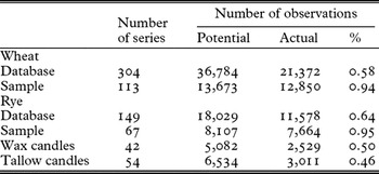
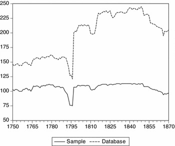
This preliminary work has yielded 480 ‘basic’ series of prices, referring to 304 markets, for wheat, 243 for rye (for 149 markets), 54 for tallow and 42 for wax candles (both for as many markets). It is thus often possible to piece together a series for a given city from different sources. In a small number of cases, the level of prices for the same market/year differs enough to entail a substantial discontinuity if simply spliced. In these cases, longer series have been used as base, and shorter series have been used to extrapolate them (forward or backwards). Even with all possible adjustments and interpolations, the database still features a very high proportion of missing observations – between a half and a third (Table 1, percentage column). Only a small minority of series (22 series for wheat, 28 for rye and none for candles) runs for the whole period 1750–1870 without a single missing observation. Such a sample would hardly be meaningful. Thus, as a compromise, the ‘baseline’ sample of markets includes all price series with at least three-quarters of observations over the whole period – i.e. 91 out of 121. This procedure cuts the number of markets by almost two-thirds, but it reduces the share of missing observations from almost 40 per cent to about 6 per cent (Table 1, row ‘sample’). As Figure 1 shows, the number of markets for wheat is fairly constant over time: it drops to a minimum 75 in 1794–6, but in all other years it ranges from 97 to 113.Footnote 5

Number of available observations: wheat prices

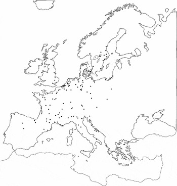
As Map 1 shows, the geographical coverage for wheat is fairly good for western and central Europe and the northern shore of the Mediterranean, while it is much less thorough for the eastern and south-eastern parts of the continent. The whole Russian empire, about a third of the European population, is represented by Warsaw alone. The sample for rye is limited to markets in north-western and central Europe (with the solitary exception of Milan and Vercelli in north Italy), where rye was the staple cereal. For both cereals, a chi-square test soundly rejects the hypothesis of equality between the distribution by country of markets and population, the only available proxy of the distribution of transactions.Footnote 6 Anyway, as shown in Section 5, the unbalanced geographical coverage does not affect the results for wheat.
Location of markets: long-run sample

Sampling problems are much more serious for candles than for cereals. First, it is simply impossible to keep the sample constant, as no series covers the whole period 1750–1870. Second, although the geographical coverage is fairly extensive, with series for Austria, Germany, France, Italy, Russia and Spain, the sample is highly unbalanced. British markets (Beveridge Reference Beveridge1965) account for between a quarter and a half of the series for tallow candles in the eighteenth century and Swedish markets (Jorberg Reference Jorberg1972) for about four-fifths of the total for both wax and tallow candles after 1803. The problem is tackled, somewhat crudely, by simply averaging all prices for Sweden and the United Kingdom and by using the result as a single series, to obtain an ‘adjusted’ sample.
4. The integration of the wheat market: a long-term view
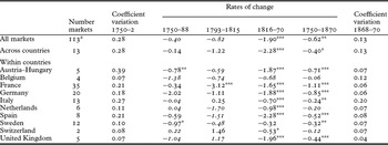
In the early 1750s wheat in Lucerne was 4.6 times more expensive than in Acquaviva delle Fonti in southern Italy, and the average price in the five most expensive markets of the continent was three times higher than in the five least expensive ones. More than one century later, in 1866–70, the two ratios were down to 2.6 and 1.6. The statistical analysis confirms the extent of integration: the σ coefficient (eq. 2) is negative and significant (Table 2, column 1750–1870). Prices converged across countries and also within all ‘countries’ in but three of them: Belgium, the Netherlands and Switzerland. In these cases, not only are the σ coefficients insignificant, but the series are stationary as well (coefficients in italics).
Rates of σ-convergence: wheat prices

*significant at 10%; **significant at 5%; ***significant at 1%.
aincluding one market each for Portugal, Russia and Denmark.
Sources: see text.
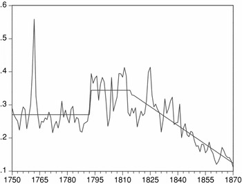
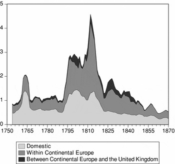
The integration process was anything but steady. A visual inspection of the coefficient of variation (Figure 2) highlights four different stages, three of which appear as separate columns in Table 2.
Trends in the coefficient of variation of wheat prices: ‘long-run’ sample 1750–1870

(i) There was little or no evidence of the development of an integrated ‘European’ wheat market in the second half of the eighteenth century.Footnote 7 The series is stationary and the σ-coefficient is not significant. Prices seem to have converged in Austria–Hungary and Sweden, but these results are not robust to changes in the list of markets.Footnote 8
(ii) The early 1790s marked a dramatic change. The average coefficient of variation for all markets jumps by two-thirds, from 0.23 in 1787–9 to 0.38 in 1793–5. Part of this jump reflects the sharp fall in the number of series, but the increase remains very large (51 per cent) also for a smaller but perfectly homogenous sample of 75 series. The Quandt-Andrews test suggests that 1793 is the strongest break point throughout the whole period 1750–1870. Consistently with the conventional wisdom, most action was on the international scene. The cross-country coefficient increased as much as the overall one, while within-country dispersion increased substantially only in Spain and, somewhat oddly, in the United Kingdom, while it decreased in Sweden.
(iii) During the French Wars, price dispersion remained high, with huge fluctuations which continued even after Waterloo. In 1824–5, the coefficient almost reached the peak of the early 1800s. The standard statistical tests for breaks do not yield clear-cut results, so ultimately the year 1815 has been chosen for its obvious political relevance.Footnote 9 As Table 2 shows, most country series are stationary, and almost all σ-coefficients are not significant. The exception, France, depends on the very high dispersion in 1793–4, when the political situation was extremely turbulent and the economic situation featured a very high inflation and a massive state intervention to fight it, the so called Maximum (Miller Reference Miller1999).Footnote 10
(iv) After 1825, price dispersion began to decline steadily. It returned permanently to its pre-war levels by the late 1830s and after this prices went on converging until a minimum at the end of the period. Integration was somewhat faster across countries than within them. The rates of σ-convergence in domestic markets varied a lot, but only in Sweden and Belgium were they not significant. Results are robust to changes in dates and in market coverage (Federico Reference Federico2008).
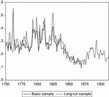
How did integration compare with later developments within Europe and in the Atlantic economy? It is possible to extend series for 32 markets of the sample to 1914 with data kindly provided by David Jacks.Footnote 11 Before 1870 the coefficient of variation for this ‘long-run’ sample reproduces almost perfectly the ‘baseline’ one (Figure 3), and thus one can be confident that it is fairly representative also of trends after 1870.
Trends in the coefficient of variation of wheat: long-run analysis 1750–1914

For a while the protectionist backlash of the late 1880s and early 1890s pushed the dispersion back to the levels of the late 1830s and early 1840s – i.e. not far from those of the eighteenth century. However, prices converged again in the first years of the twentieth century and the coefficient of variation on the eve of the World War I dispersion was only about 50 per cent higher than in the 1860s. The level of integration of the European market peaked in the early 1920s (Federico and Persson Reference Federico, Persson, Hatton, O'Rourke and Taylor2007) and collapsed in the early 1930s, never to be attained again.
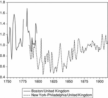
By contrast, the first half of the nineteenth century did not advance the integration of the Atlantic economy. Before the 1850s there is no evidence of price convergence between the east coast of the United States and the United Kingdom (and thus, by inference, the rest of Europe).Footnote 12 The ratios fluctuated wildly without any significant trend (Figure 4)
Price ratios: wheat, United States/United Kingdom

As O'Rourke and Williamson (Reference O'Rourke and Williamson1999, p. 2) put it, ‘the really big leap to more globally integrated commodity and factor markets took place in the second half of the century’.
5. Robustness checks
Even if our data are superior in size and, arguably, in quality to those commonly used in the literature, the sample still suffers from three shortcomings: errors in data, missing observations and unbalanced geographical coverage. This section addresses each of these shortcomings in turn, by comparing the ‘baseline’ series of the coefficient of variation with alternative ones, computed with an appropriately modified database.
(i) As stated in Section 2, price series can be biased systematically by the resort to non-market sources and/or by the presence of quality differentials, either permanent or changing over time. It is possible to rule out systematic changes in relative quality before the diffusion of ‘industrial’ varieties of seeds in the late nineteenth century (Federico Reference Federico2005), but not permanent quality differentials. In fact grading was introduced in the main markets only towards the end of the nineteenth century and sources do not report information on the quality of wheat or use generic labels (‘mercantile’, ‘good’ and so on).Footnote 13 The bias from use of private sources can be avoided simply by omitting the series. The alternative sample, labelled ‘high-quality sample’, excludes also any other series whose quality appears questionable (e.g. series obtained by averaging few monthly observations). The sample consists of a maximum of 90 series – i.e. about a quarter less than the ‘baseline’ one.
The data are also subject to unsystematic errors in the original sources and in the complex process to convert prices into a common currency and unit of weight (collection of prices, elaboration before publication, further processing of secondary sources). These errors can be assumed to be randomly distributed, in the absence of any evidence to the contrary. One can plausibly assume that the most egregious mistakes appear as outliers in the database and drop them altogether (‘no-outliers sample’). An observation will be defined as an outlier if it exceeds two standard deviations from the mean. Dropping all the 560 outliers reduces the total number of observations by 4.5 per cent only.
(ii) The problem of missing observations can be tackled in two different ways. First, it is possible to use more restrictive criteria for the inclusion of a series. Accepting only series with no more than 5 per cent missing observations (6 out of 121) yields a ‘consistent’ sample with 69 series and 8,186 observations (98.1 per cent of the potential).
As an alternative, one can impute the missing observations following a three-step procedure:
(a) compute the ratio Rit=xit/μt for all available observations for the i-th market;
(b) compute RiAV=(ΣRit+m+3+ΣRit−n−3)/6 as the average of the ratios for the six years straddling the missing observation(s) Rit−n. . .Rit+m (e.g. to impute the missing values for Prague in 1770–71, RiAV is obtained as a simple average of ratios for 1767–1769 and 1772–1774);Footnote 14
(c) compute the missing price as Pit=μ*t RiAV
This procedure yields an ‘integrated sample’ with as many series as the baseline one, but with no missing data.
(iii) A simple way of increasing the representativeness of the sample is to increase the number of series, especially for under-represented countries. Many series which are too short to be included from the ‘baseline’ are useful for building alternative samples. An earlier extended version of this article (Federico Reference Federico2008) considers samples for 1750–93 (‘Late eighteenth century’, with 140 series), 1789–1820 (‘French Wars’, with 125 series) and 1797–1870 (‘Early nineteenth century’, with 183 series).Footnote 15 Results are very close to those of the ‘baseline’ ones.
This method may not convince the truly sceptical reader, as many of the additional markets are located in already well-represented countries. The only way to have a statistically representative sample is to pare down the number of markets until the distribution is not different from that of the universe (i.e. the population of the countries of the sample). The largest feasible ‘representative’ sample consists of 30 series, six for France and Germany, five for Austria-Hungary, four for Italy and the United Kingdom, three for Spain and one for Belgium.Footnote 16
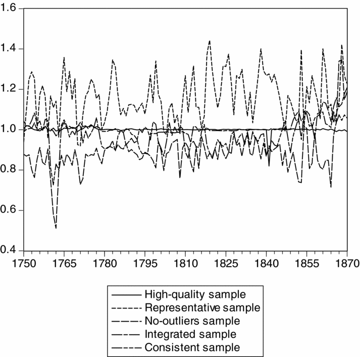
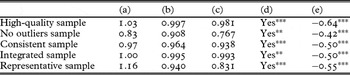
The differences between these alternative series and the ‘baseline’ one are fairly small (Figure 5). The average ratio to the ‘baseline’ sample is very close to one in three cases out of five (Table 3 column, a), the coefficients of correlation are quite high, both in levels (Table 3, column b) and in first differences (Table 3, column c). Above all the differences are totally trendless: the series are cointegrated at least at 5 per cent (Table 3, column d) and the rates of σ-convergence are never significantly different from the ‘baseline’ ones (Table 3, column e).
Robustness tests, wheat prices: ratios to the baseline series
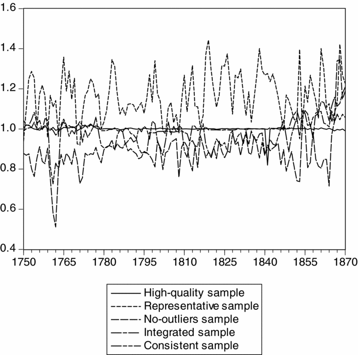
Robustness tests: differences between baseline and alternative series

Significant at *10%; **5%; ***1%.
In short, although the database is far from perfect, the main results seem remarkably robust.
6. On the causes of integration: some insights from variance analysis
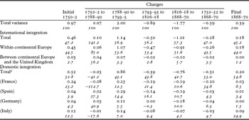
Table 4 (and Figure 6) reports the results of the basic variance analysis. It distinguishes variance ‘within continental Europe’ (i.e. the convergence or divergence of the mean price for each country towards the continental average), variance ‘between continental Europe and the United Kingdom’ and the cumulated domestic variance for the ten countries (plus data for selected countries). For each of these sources, it reports the initial and final standardized variance (see Appendix), the absolute changes by period and the contribution to overall change in variance (italic, lower row). For instance, the variance ‘within continental Europe’ (0.43 standardized points) accounted for 45 per cent of the total in 1750–2. It increased by 0.06 points to 1788–90 and this change accounted for 85 per cent of the total increase in variance in that period. From 1788–90 to 1793–5 it rose by a further 1.07 points, to a maximum of 1.56 points (54 per cent of total increase), and so on.
Variance analysis, wheat prices: long-term changes

aSum of domestic integration in Austria–Hungary, Belgium, France, Germany, Italy, the Netherlands, Spain, Sweden, Switzerland and the United Kingdom.
Sources: see text.
Variance analysis, wheat prices

Domestic and international integration contributed by almost the same amount to long-term change (from 1750–2 to 1868–170), but this not the case for changes in the four periods, which are in absolute terms between two and ten times larger than the long-run. Medium-term changes were dominated by movements in the international variance, most notably by changes ‘within continental Europe’. A further decomposition by country shows that this mostly reflects convergence (or divergence) of marginal countries, most notably Spain, towards the European average.Footnote 17 Core countries contributed less to these changes because their prices remained much closer to the continental average, a typical instance of regression towards the mean. By contrast, trends in domestic integration depended mostly on changes in big countries. For example, France only accounted for between a quarter and a half of the total. The United Kingdom is omitted because its contribution was minimal.
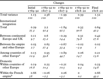
The variance analysis is most useful in analysing the impact of specific, time-discrete events, such as the French Wars. French occupation is said to have fostered the creation of an integrated market within the empire, whilst raising high barriers to trade with the rest of Europe, culminating in the proclamation of the Continental Blockade in November 1806. Trade in wheat was exempt from the harshest prohibitions, but the effects of France's ascent to European domination are nevertheless quite clear (Table 5).Footnote 18 Variance in all sources outside the empire, including domestic variance in other countries, increased significantly. On the other hand, prices within the empire did indeed converge, as the negative sign shows, but the effect was negligible.
Variance analysis, wheat prices: the effect of the French Wars

aPrussia, Austria–Hungary, Sweden, Russia, Spain and Portugal.
bFrance (within its pre-revolutionary borders), Switzerland, Netherlands, Italy, Belgium and the so-called Confederation of the Rhine in West Germany.
Source: see text.
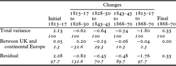
The end of the French Wars also marked a major change in trade policy (Federico Reference Federico2009). Producers feared that the return to normalcy would cause wheat prices to fall from their highly remunerative wartime levels. Thus, they claimed and, for the first time, obtained protection from imports. As early as 1815, the United Kingdom prohibited imports if domestic prices did not exceed 80 shillings per quarter, France introduced a sliding scale in 1819, Spain prohibited imports altogether in 1820, and so on. However, these protectionist policies did not last for long, in clear contrast to the late century backlash. The 1828 British Corn Laws, which were to be repealed in 1843, were decidedly more liberal than their 1815 version (Sharp Reference Sharp2006). Other countries followed suit from the mid 1830s on, as part of a long-run pan-European process of trade liberalization (Accominotti and Flandreau Reference Accominotti and Flandreau2008). The twin roles of the United Kingdom as a major importer of grain and as leading economy in Europe make the effect of the change in Corn Laws a prime candidate for a variance analysis of the impact of trade policy. To this aim, Table 6 isolates convergence between the United Kingdom and continental Europe from all other sources of changes in variance.
Variance analysis, wheat: the effect of Corn Laws

Source: see text.
Convergence between the United Kingdom and the continent, although not so important for long-run trends (Table 4), accounts for a substantial share of medium-term changes in total variance. Without the 1815 Corn Laws, in the 1820s price dispersion all over Europe would have fallen by a third more and the 1828 liberalization accounted for a third of total convergence in the next fifteen years. The impact of their final repeal is smaller but still noticeable.
These two examples assume implicitly that political events were the only determinant of changes in integration. This assumption would be the more true the smaller the changes in transaction costs and/or in the efficiency of the market. We know very little about the operational efficiency of wheat markets or about the costs of information exchange. The laying of telegraph lines from the 1840s on boosted the speed of the circulation of information (Hoag Reference Hoag2006), but the movement had started earlier (Kaukiainen Reference Kaukiainen2001). Anyway, faster and cheaper information is more likely to have affected arbitrage than long-term convergence. In contrast, one would expect convergence to have been heavily influenced by changes in transport costs which are routinely measured by the ratio of freights to wheat prices, the so-called ‘freight factor’ (Hummels Reference Hummels2007).Footnote 19 Evidence for the late eighteenth century is admittedly scarce and somewhat mixed. Freight factors remained roughly constant both for wheat imports from Russia to the Netherlands (Knoppers Reference Knoppers1976) and for the sea-born domestic trade in the British Isles (Harley Reference Harley1988).Footnote 20 Labrousse (Reference Labrousse1933, pp. 125–33) for France and Fouquet (Reference Fouquet2008) for the United Kingdom suggested that road transport costs had remained constant, while Albert (Reference Albert1972) found a small decline in official rates in the United Kingdom. Wheat prices in both countries increased, by half in the UK and by one-third in France – so in theory the freight factor should have declined. The cost of domestic transportation must have been reduced also by the construction of canals, which were cheaper to use than roads.
Trends in transportation costs in the first half of the nineteenth century are much better known. ‘Freight factors’ for sea transport fluctuated widely in the short run, but in the long run they declined substantially (North Reference North1958; Harley Reference Harley1988; Harlaftis and Kostelenos Reference Harlaftis and Kostelenos2007; Klovland Reference Klovland2006). Transporting wheat to London or the Mediterranean cost around 30–40 per cent of the price in the Baltic or the Black Sea in the 1830s and only 10–15 per cent in the late 1860s. The cost of inland transportation seems to have fallen as well. The freight factor decreased for water-borne traffic on the Rhine (Horlings Reference Horlings1995) and on French and Swedish canals (Toutain Reference Toutain1967; Thorburn Reference Thorburn2000). Railway rates were cut in Italy (Federico Reference Federico2007), and costs per ton/mile, a less precise measure, fell in France (Toutain Reference Toutain1967) and the United Kingdom (Hawke Reference Hawke1970). Progress was much less evident in road transportation. Toutain (Reference Toutain1967) hypothesizes that in France the unit cost remained constant between the 1820s and the 1860s, causing the ‘freight factor’ to decrease by about a tenth. In Sweden, unit costs doubled from 1830 to 1873 and the ‘freight factor’ increased by a half (Thorburn Reference Thorburn2000). Anyway, the average cost of transportation was falling because agents could substitute canals for roads. Thorburn (Reference Thorburn2000) stresses how the opening of new canals in 1819 and in 1832 greatly fostered price convergence of hitherto isolated markets towards the Stockholm ones. For the same reason, one would expect a positive effect of railway building, if they substituted roads (while canals were on average still cheaper).Footnote 21 Indeed, Jacks (Reference Jacks2006) and Keller and Shiue (Reference Keller and Shiue2008) find a positive relation between pairwise integration between markets and a dummy for the existence of railway connection between the cities in question.Footnote 22
One could conclude that transport costs may have had a modest positive effect on integration before the 1780s, possibly offsetting the negative effect of wars and other political events, and a much stronger positive effect in the first half of the nineteenth century. On the other hand, the decline in the freight factor was concentrated in the 1850s and 1860s. These decades also featured the first massive wave of railway building outside the United Kingdom. By 1850, the British network had reached about one-third of its 1913 extension, but in other countries the share ranged from less than 1 per cent (Spain) to 18 per cent (Belgium), no line having been opened in Portugal and Sweden (Mitchell Reference Mitchell1998, table G1). By default, one has to suppose that the convergence from the 1820s to the late 1840s was determined mostly by changes in trade policy. Indeed, in those years, convergence across countries accounts for about 90 per cent of the total.
7. Candles and rye
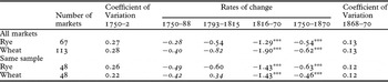
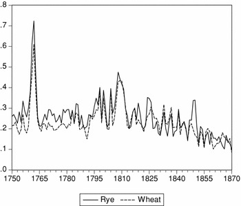
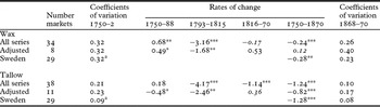
On average over the whole period, rye cost about 0.7 times as much as wheat, tallow candles 6.2 times, and wax candles 21.5 times per unit of weight. Thus, one would expect initial price dispersion to be (slightly) higher for rye and significantly lower for tallow and wax candles and integration to be faster for rye and slower for candles. The case of rye, by and large, confirms expectations (Table 7 and Figure 7). In the 1750s the coefficient of variation for the same sample of markets was about a quarter higher than for wheat and over the whole period convergence was a bit faster, although the difference is not significant.
Rates of σ-convergence: wheat and rye prices

Significant at * 10%; ** 5%; *** 1%.
Sources: see text.
Trends in the coefficient of variation: wheat and rye prices

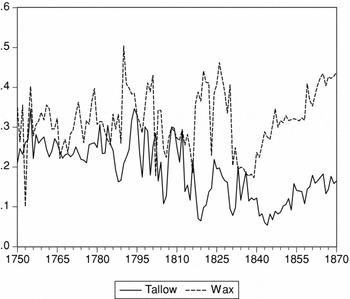
The case of candles is different. In the 1750s the coefficient of variation was as high for tallow candles as for wheat and was even higher for wax candles. Furthermore, once adjusted for the unbalanced geographical coverage, there is very little, if any, evidence of σ-convergence. Coefficients for wax candles fluctuated widely without any trend (Figure 8 and Table 8). The series for tallow candles does show some convergence in the long run, but the movement concentrates in the period of the French Wars, hardly the best time for the integration of the European market. Indeed, this specific result is not robust to small changes in the dates and in the sample. In both cases, prices diverged from the mid 1840s – so that the coefficient of variation for wax candles in the 1860s exceeded 0.4, as in the 1790s and in the mid 1820s, and it was three times higher than the coefficient for wheat. Price dispersion increased also in the European market for tallow candles, although not in the Swedish market.Footnote 23
Trends in the coefficient of variation: prices of wax and tallow candles, ‘adjusted’ sample, 1750–1870

Rates of σ-convergence: prices of candle

a1803–5.
Significant at *10%; **5%; ***1%.
In brief, the market for candles was consistently less integrated than expected, given relative prices, and, unlike for cereals, the levels of integration did not increase over time. To be sure, trade was much less developed for candles than for wheat, and thus, in all likelihood, information was less abundant. However, this is not a sufficient explanation for such a big difference. The fall in transport costs benefited trade in candles as well and profits from arbitrage in candles should have been as appealing as those from arbitrage in wheat. The reason for the difference between cereals and candles must be sought in the size of quality differentials. They increased dispersion and made arbitrage more difficult and risky. Technical progress in candlemaking caused these differentials to widen from the 1840s on (Fouquet Reference Fouquet2008; Eveleigh Reference Eveleigh2003).
8. Conclusions
The main results of this article may be summarized as follows:
(i) In the long run wheat and rye markets experienced a massive process of integration, with dispersion reaching an (almost) all-time low in the late 1860s.
(ii) Price dispersion remained roughly constant in the second half of the eighteenth century and increased sharply in the early 1790s. It was back at its pre-war level by the 1830s, so that all the further increase to the 1860s was additional σ-convergence into uncharted territory.
(iii) Both domestic and international markets contributed roughly to the same extent to long-run integration, but the latter contributed decidedly more to medium-run changes.
(iv) Most changes seem to have been driven by political events, such as the French Wars, the protectionist backlash of the 1820s and subsequent trade liberalization. Trade in wheat was substantially free from duties from the 1850s and thus the further convergence reflects mostly the fall in transportation costs, including the effect of railways.
(v) The case of candles shows how conclusions based on cereals might not be extended easily to manufactures. This case is interesting not only for its relevance as a consumer good but also as a warning sign against simplistic inferences from cereals. Quality may not be an issue for wheat, or for other homogeneous goods, but it was undoubtedly a major obstacle to the integration of the market for manufactures, where quality differentials were much larger and shifted over time as a consequence of technical progress.
This analysis suggests four general points:
(a) The quest for an optimal measure of integration is still open and must be supported by more theoretical awareness about the different concepts of integration.
(b) Although the data will never be sufficient to address all potential issues, the sources are now much more plentiful than assumed so far, even for cereals, the workhorse of the literature. A fortiori, a further systematic effort on other products is overdue.
(c) An important issue, which will be very difficult to address, is the integration of local markets. All available price series refer to urban markets, usually to major cities. Yet price convergence between the latter and the surrounding villages, and between villages and single farms, must have contributed substantially to overall integration. Farmgate prices are very difficult to find, and one will have to resort to farm records and other microeconomic sources (Rothenberg Reference Rothenberg1992).
(d) Last but not least, it is time to go beyond pure measurement. The work on causes of integration is promising, albeit still preliminary, while welfare effects have so far been totally neglected. Scholars assume that market integration played a key role in modern economic growth, but they should buttress this claim with some figures.
In short, the rewards from further research can be substantial: there is much more to the history of market integration than the triumph of globalization in 1870–1913 and its reversal by the interwar backlash.
Acknowledgements
The author thanks two referees, Kevin O'Rourke and participants at seminars in EUI, LSE, Oxford, Science-Politiques (Paris) and at the 6th conference of the European Historical Economics Society for comments on an earlier version of this paper. The research was funded by the ERC project 230484 ‘Market integration and the welfare of Europeans’.
Appendix
This appendix deals with two issues: (i) the biases from quality differentials, and (ii) the allocation of changes in total variance among different sources.
(i) The coefficient of variation at time t would measure exactly the dispersion of prices if all data refer to the same quality (pitQ):

Unfortunately, as noted, the available prices (pit) may differ from the quality-adjusted ones, because the quality differs from the reference one and/or because they do not refer to market transactions. Let us assume this difference to be ξit (ξit = pit− pitQ) and define the reference quality as a composite one so that Σ ξit = 0 (i.e. μt = μtQ).Footnote 24 The ‘ideal’ coefficient can then be rewritten as

which differs from the real one (eq. 1)

by the amount of the quality premiums ξit. A comparison between (4) and (5) shows that

while

In other words, the coefficient of variation would be biased upwards if the difference between the registered price pi and the ‘true’, quality-adjusted one piQ, is positive (i.e. the quality of the quoted wheat is better than the ‘reference’ one) in high-price markets, or if it is negative in low-price markets. The coefficient would be biased downwards in the opposite case, but only if

i.e. if the difference in quality-adjusted prices exceeds the quality gap in absolute value. Therefore, the coefficient of variation is more likely to be upward than downward biased. This bias would be smaller, the greater the differences in quality-adjusted price differentials relative to quality differentials. This implies that quality differentials are a problem especially in highly integrated markets.
This reasoning is broadly similar for changes in quality over time. Let us assume for the sake of simplicity that at the beginning there are no quality differentials (ξit = 0) and that quality-adjusted prices remain constant (pitQ = pit+1Q) – i.e. that CVtQ = CVt+1Q. A change in relative quality from time t to time t+1 in the ith market adds a quality differential term (ξit+1) and affects proportionally the overall average. Thus the ‘actual’ coefficient of variation at time t + 1 becomes

An improvement in relative quality ([ξit+1 +1/n ξit+1]>0) would bias upwards the coefficient of variation (CVt+1 > CVt+1Q) in high price markets (pitQ > μtQ), but it would bias it downwards in low price ones(pitQ < μtQ). The effect of a worsening of relative quality ([ξit+1 +1/n ξit+1] < 0) would be the opposite and the net effect is unpredictable. A perfect compensation is possible.
(ii) Let us assume markets are divided into m groups, according to political boundaries or any other relevant criteria. Total variance at time t is

where subscripts 1. . .m refers to groups and W to the ‘world’ and n is the number of markets in each group. The first term measures the dispersion between groups, and the others measure the dispersion within each group. Comparison across time or space is easier if data are normalized by dividing variance by the number of markets times the average price:

Different layers of grouping can also be added. For instance, to study the impact of trade policy, one can distinguish free trade (FC) and protectionist countries (PC). In the case of four countries, the formula becomes, omitting time superscripts for simplicity,

The first row measures the convergence (or divergence) between free trade and protectionist countries, the second and third, the convergence within each area (i.e. between protectionist countries 1 and 2 and free-trade countries 3 and 4) and the remaining ones, the ‘domestic’ convergence within each country.
It is possible to measure the contribution of each component to total change by letting only its variance change, while keeping variance from all other sources at its initial level. For instance, the contribution of price convergence within group 1 (or Con(1)) to changes in total variance from t to t+1 can be measured by the ratio

Where CVar(1)t+1 is