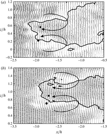
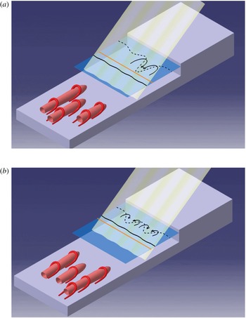
1 Introduction
Shock wave–boundary layer interactions (SWBLI) occur at many locations on high-speed vehicles, such as supersonic inlets, nozzles, transonic airfoils and scramjet engines. These interactions, especially the ones leading to shock-induced separation, are typically unsteady in nature and can lead to large fluctuating pressure and thermal loads on the structure. Motivated by these practical issues, there have been a number of studies on SWBLI as summarized in the reviews of Dolling (Reference Dolling2001), Knight et al. (Reference Knight, Yan, Panaras and Zheltovodov2003), Dussauge & Piponniau (Reference Dussauge and Piponniau2008) and Clemens & Narayanaswamy (Reference Clemens and Narayanaswamy2014). An important question with the shock unsteadiness that has been debated extensively is the source of the low-frequency shock oscillations (Dolling Reference Dolling2001; Dussauge & Piponniau Reference Dussauge and Piponniau2008; Clemens & Narayanaswamy Reference Clemens and Narayanaswamy2014). Driven by this debate, there have been a number of studies that have investigated SWBLI recently, with most of these studies focusing on the compression ramp or impinging/reflecting shock cases. In the present work, we experimentally study the SWBLI in flow over a forward-facing step (FFS) geometry, as it represents a simple geometry with a large separation bubble, and may be thought of as an extreme case of a compression ramp with a ramp angle of
 $90^{\circ }$
. There have been a few early studies on this geometry, which have been reviewed by Zukoski (Reference Zukoski1967), but almost no recent detailed study.
The low-frequency oscillations of the shock in SWBLI are typically approximately two orders of magnitude smaller than the characteristic frequencies of the incoming boundary layer (
 $U_{\infty }/\unicode[STIX]{x1D6FF}$
) (Clemens & Narayanaswamy Reference Clemens and Narayanaswamy2014). Broadly speaking, there are two schools of thought regarding the origin of these low-frequency large-scale shock oscillations, as discussed in Ganapathisubramani, Clemens & Dolling (Reference Ganapathisubramani, Clemens and Dolling2007), Dussauge & Piponniau (Reference Dussauge and Piponniau2008) and Clemens & Narayanaswamy (Reference Clemens and Narayanaswamy2014). One is the upstream influence, which attributes these shock oscillations to the structures within the incoming boundary layer, while the other is the downstream influence, which attributes these oscillations to the instabilities of the separation bubble. There have been studies that have shown support for both viewpoints.
Many studies suggest that structures within the incoming boundary layer are responsible for the low-frequency shock motion. For example, Andreopoulos & Muck (Reference Andreopoulos and Muck1987) and Erengil & Dolling (Reference Erengil and Dolling1991) studied shock foot motion in supersonic flow over a compression ramp using unsteady pressure measurements and observed a clear correlation between the pressure fluctuations under the shock foot and the incoming boundary layer. Beresh, Clemens & Dolling (Reference Beresh, Clemens and Dolling2002) and Hou (Reference Hou2003) showed, using simultaneous pressure and particle image velocimetry (PIV) measurements, that the upstream boundary layer velocity profiles were fuller when the shock foot was downstream, as compared to when it was upstream. Ganapathisubramani et al. (Reference Ganapathisubramani, Clemens and Dolling2007) and Ganapathisubramani, Clemens & Dolling (Reference Ganapathisubramani, Clemens and Dolling2009) showed, using PIV measurements in the streamwise–spanwise plane, the presence of low- and high-speed streaks within the boundary layer and the undulations in the spanwise separation line induced by these regions. Ganapathisubramani et al. (Reference Ganapathisubramani, Clemens and Dolling2009) also showed the temporal evolution of the shock and separation line using high-speed PIV at 6 kHz. For the impinging–reflecting shock case, Humble et al. (Reference Humble, Elsinga, Scarano and Van Oudheusden2009) also found similar undulations of the shock corresponding to low- and high-speed regions within the boundary layer from tomographic PIV.
A number of studies have also shown evidence that the downstream source, from the separation bubble, is more prominent. For example, pressure measurements of Thomas, Putnam & Chu (Reference Thomas, Putnam and Chu1994) for a compression ramp and Dupont, Haddad & Debiève (Reference Dupont, Haddad and Debiève2006) for the impinging–reflecting shock case, show that the pressure fluctuations at the foot of the shock are correlated and out of phase with the fluctuations beneath the separation bubble. Piponniau et al. (Reference Piponniau, Dussauge, Debiève and Dupont2009) have shown from PIV measurements that the position of the shock is more upstream for large separation bubbles, and more downstream when the bubble is small. They also modelled the low-frequency shock motion based on the entrainment and recharge mechanism of the separated shear layer and showed a good comparison with their own as well as with several other studies reported in the literature from Mach 0 to 5. Wu & Martin (Reference Wu and Martin2008) and Priebe & Martin (Reference Priebe and Martin2012) have shown from direct numerical simulation (DNS) of Mach 2.9 flow over a compression ramp that the shock motion is related to the breathing motion of the separation bubble. Priebe & Martin (Reference Priebe and Martin2012) point out that this breathing bubble motion is reminiscent of the unstable global mode obtained by Touber & Sandham (Reference Touber and Sandham2009) from a linear stability analysis of the mean flow in a reflected shock interaction.
A lot of the detailed studies on SWBLI to date have investigated either the unswept compression ramp or the impinging–reflecting shock. Other geometries such as cylinders, forward-facing step (swept and unswept), swept compression ramp, blunt and sharp fins have also been studied (Clemens & Narayanaswamy Reference Clemens and Narayanaswamy2014), although there have been fewer detailed studies. As stated by Smits & Dussauge (Reference Smits and Dussauge2006) and Clemens & Narayanaswamy (Reference Clemens and Narayanaswamy2014), the unsteady shock motions in these different flow configurations show similarities. In the present work, we present results from an experimental study of supersonic flow over an unswept FFS. This geometry represents a simple configuration with a large separation bubble, and may also be thought of as an extreme case of the compression ramp geometry. Zukoski (Reference Zukoski1967) reviewed early work on supersonic flow over a forward-facing step, highlighting the large separation bubble formed ahead of the step. He showed from a compilation of mean wall pressure data that the separation distance ahead of the step (
 $x_{sep}/h$
) was nearly independent of the Mach number and the step height to boundary layer thickness (
 $h/\unicode[STIX]{x1D6FF}$
), for
 $(h/\unicode[STIX]{x1D6FF})>1.2$
. A number of these early studies report on mean pressure ahead of the step, while a few also report on unsteady measurements of wall pressure (Kistler Reference Kistler1964) and velocity from hot-wire (Gran Reference Gran1970; Behrens Reference Behrens1971), with these unsteady measurements showing the presence of low-frequency shock motions. Compared to the supersonic case, there have been more studies on the subsonic flow over a FFS, including both experimental studies (Moss & Baker Reference Moss and Baker1980; Martinuzzi & Tropea Reference Martinuzzi and Tropea1993; Camussi et al.
Reference Camussi, Felli, Pereira, Aloisio and Di Marco2008; Sherry, Jacono & Sheridan Reference Sherry, Jacono and Sheridan2010; Pearson, Goulart & Ganapathisubramani Reference Pearson, Goulart and Ganapathisubramani2013) and numerical or flow stability studies (Wilhelm, Härtel & Kleiser Reference Wilhelm, Härtel and Kleiser2003; Marino & Luchini Reference Marino and Luchini2009; Lanzerstorfer & Kuhlmann Reference Lanzerstorfer and Kuhlmann2012). In the incompressible case, the role of upstream perturbations on the instability of the separation bubble has recently attracted attention, as discussed by Lanzerstorfer & Kuhlmann (Reference Lanzerstorfer and Kuhlmann2012) in the laminar case and by Pearson et al. (Reference Pearson, Goulart and Ganapathisubramani2013) for the turbulent case, the latter study involving time-resolved PIV measurements.
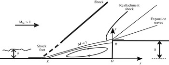
We study in the present work a Mach 2.5 flow over a FFS. The focus of the work is the flow ahead of the step, in particular, the unsteady interactions between the shock, the boundary layer and the separation bubble. Figure 1 shows the schematic of the geometry showing the main flow features and the parameters in the problem, namely, the free-stream Mach number
 $M_{\infty }$
, the step height
 $h$
and the incoming boundary layer thickness
 $\unicode[STIX]{x1D6FF}$
. In the mean, a large separation bubble forms in front of the step, along with a separation shock ahead of it, as shown in the schematic. The primary geometrical parameter in the problem is the ratio of the step height to the incoming boundary layer thickness,
 $h/\unicode[STIX]{x1D6FF}$
, which is fixed at 2 in the present study. This was chosen as it keeps both
 $h$
and
 $\unicode[STIX]{x1D6FF}$
comparable, while at the same time, the step protrudes out of the boundary layer, as in the compression ramp cases, mimicking in some way the well-studied case of the compression ramp. Further, as stated earlier, Zukoski (Reference Zukoski1967) in his review of supersonic flow over a FFS has shown that the normalized separation point location (
 $x_{sep}/h$
) and the mean pressure profile are nearly independent of the step height for
 $h/\unicode[STIX]{x1D6FF}>1.2$
. Hence, the present study could be thought of as representative of steps that are bigger than the boundary layer thickness. Throughout the present study, the mid-span of the bottom corner of the step is taken as the origin (O), as indicated in figure 1. The
 $x$
-axis is in the streamwise direction,
 $y$
-axis is in the cross-stream or wall-normal direction and the
 $z$
-axis is in the spanwise direction. Results are presented from detailed PIV measurements in two orthogonal planes, one perpendicular to the test-section bottom wall (cross-stream or wall-normal,
 $x$
–
 $y$
) plane, and the other in the spanwise plane (
 $x$
–
 $z$
) to gain a reasonable picture of the whole flow field.
Schematic showing the main parameters in supersonic flow over an unswept FFS. In the figure,
 $M_{\infty }$
is the free-stream Mach number,
 $\unicode[STIX]{x1D6FF}$
is the incoming boundary layer thickness and
 $h$
is the step height, with
 $h/\unicode[STIX]{x1D6FF}$
being the main geometrical parameter. In this case, the flow separates ahead of the step forming a large separation bubble with a separation shock ahead of it. Also shown in the figure is the sonic line (
 $M=1$
) and the bow shock and expansion fan that can form close to the step corner.

The layout of the paper is as follows. In § 2, we give details of the experiment and instrumentation. Measurements characterizing the undisturbed boundary layer are also presented, along with measurements showing that the velocity fields in the central part of the FFS model, for the cases studied, are nearly independent of the spanwise length of the model. This is followed by § 3, where we present the time-averaged PIV velocity field in the cross-stream or wall-normal (
 $x$
–
 $y$
) plane and in the spanwise (
 $x$
–
 $z$
) plane along with the spectra of the wall pressure fluctuations. In §§ 4 and 5, we present unsteady aspects of the velocity field in the wall-normal and the spanwise planes, respectively. In both these sections, we present instantaneous fields and characterize the locations and changes in the shock, separation bubble size, and the incoming boundary layer fluctuations. A discussion of the results obtained is presented in § 6 followed by the conclusions in § 7.
2 Experimental details
The experiments were done in an open circuit supersonic blow-down tunnel at the Department of Mechanical Engineering, Indian Institute of Science. All experiments presented were done at a free-stream Mach number of 2.54. The tunnel test section had a cross-section of 100 mm
 $\times$
80 mm and a length of 350 mm. Air for the tunnel was obtained from a 6 m
 $^{3}$
storage tank containing air at 30 bar, which was filled using two 20 HP electric powered two-stage compressors. Before storage, the compressed air was dried using refrigeration air drier to remove moisture from the air and was also passed through an oil filter. The compressed air from the storage tank entered the test section through a two-stage pressure regulation system; the first reducing the pressure from 30 bar to approximately 10 bar, and the second further reducing the pressure down to the working pressure in the settling chamber, which was approximately 3 bar. This two-stage pressure regulation was found to give a nearly constant pressure in the settling chamber of the tunnel with variations of less than 1 % during the approximately 40 second run time. Within the settling chamber, the air passed through a honeycomb and a series of fine meshes, to improve uniformity and reduce the turbulence level. This flow then passed through a Mach 2.54 convergent–divergent nozzle and reached the test section. The test-section side and top walls were made transparent to provide optical access. The free-stream velocity measured using PIV within the test section was 585 ms
 $^{-1}$
, with a turbulence level in the free stream that was lower than 1.5 % of the free-stream velocity.
2.1 Particle image velocimetry (PIV) and pressure measurements
PIV was the main technique used to study the SWBLI over the FFS. It is comprised of a New Wave 120 mJ, 532 nm dual cavity Nd-YAG laser with a repetition rate of 15 Hz, a Dantec Flowsense CCD camera of 1600
 $\times$
1200 pixel resolution and a timer card for synchronization. The laser beam was made into a sheet using sheet optics with a typical laser sheet thickness of approximately 1.5 mm. For PIV experiments, the surface of the model was painted black to help reduce laser reflection from the surface. We report on PIV measurements done in two perpendicular planes, one being in the cross-stream or wall-normal (
 $x$
–
 $y$
) plane, and the other being in the spanwise (
 $x$
–
 $z$
) plane. For wall-normal view experiments, the laser sheet entered the test section vertically from the transparent top wall to illuminate the
 $x$
–
 $y$
plane normal to the lower wall, with the camera viewing the illuminated plane through the transparent side wall. In the other case, for the spanwise view experiments, a horizontal laser sheet entered the test section through the side wall and illuminated the
 $x$
–
 $z$
plane parallel to the lower wall, with the camera viewing the flow through the transparent top wall. The PIV seeding was done using olive oil particles from a Laskin nozzle-based seeder (Raffel Reference Raffel2007), which was connected to the beginning of the settling chamber. The particle response time for the seed particles was assessed from measurements of the particles as they passed through an oblique shock, which showed that the particle response time was approximately
 $7.9~\unicode[STIX]{x03BC}\text{s}$
. The particle diameter was estimated from this to be approximately
 $0.6~\unicode[STIX]{x03BC}\text{m}$
based on the studies of Melling (Reference Melling1997).
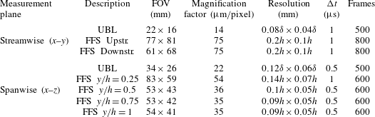
PIV measurement details for the undisturbed boundary layer (UBL) and flow over a FFS. Measurements were done in both streamwise (
 $x$
–
 $y$
) and spanwise (
 $x$
–
 $z$
) planes. FFS Upstr. and FFS Downstr. represents the PIV measurements in the
 $x$
–
 $y$
plane done upstream and downstream of the step, which were then time averaged and combined to obtain the mean data shown in figure 4(a,b). For each of the measurements, the FOV, the magnification factor, the spatial resolution corresponding to the interrogation box size (in terms of boundary layer thickness (
 $\unicode[STIX]{x1D6FF}$
) or step height (
 $h$
)), the inter-frame time and the number of PIV fields obtained are shown.

The camera and Laser were fired through the DynamicStudio software in synchronous mode at an acquisition rate of 15 Hz. The inter-frame time was set such that we obtained a particle displacement of approximately 10 pixels corresponding to the free-stream velocity. Typical inter-frame times used in the present experiments were 0.5 or
 $1.0~\unicode[STIX]{x03BC}\text{s}$
. The recorded image pairs were then processed in DynamicStudio software by adaptive correlation with 32
 $\times$
32 pixel final box size, except in the case of the undisturbed boundary layer measurements in the
 $x$
–
 $y$
plane where a final box size of 32
 $\times$
16 was used with smaller box dimension in the wall-normal (
 $y$
) direction. In all cases, 50 % box overlap was used to obtain instantaneous velocity fields. The details of the different PIV measurements done in the streamwise (
 $x$
–
 $y$
) and the spanwise (
 $x$
–
 $z$
) planes including values of the field of view (FOV), magnification (microns/pixel), resolution, inter-frame time (
 $\unicode[STIX]{x0394}t$
) and number of PIV fields obtained in each case are given in table 1. To filter out spurious vectors, a 3
 $\times$
3 local neighbourhood median-based validation using a maximum deviation allowed of 40 % of the median value was used along with a peak validation ratio of at least 1.2 between the highest and second highest correlation peaks. Spurious vectors were typically found to be less than 1 % of the total vectors in the field for
 $x$
–
 $y$
plane measurements and less than approximately 3 % of the total vectors in the field for
 $x$
–
 $z$
plane measurements, and these were substituted using the median value of the surrounding vectors. It may be noted that in all the PIV measurements done, the out-of-plane particle displacements were small compared to the laser sheet thickness as the inter-frame time was sufficiently small, resulting in the relatively small percentage of spurious vectors.
Unsteady wall pressure measurements were done using pressure transducers (Model number: LQ-062-25A) from Kulite Semiconductor Products, Inc. This transducer had a nominal diameter of 1.6 mm with the pressure sensitive diaphragm having a diameter of 1.2 mm. It was placed at two locations ahead of the step, corresponding to the approximate location of the separation shock (
 $x/h=-4.2$
) and the middle of the separation bubble ahead of the step (
 $x/h=-2.1$
). The sensitivity of the transducer was approximately
 $0.58~\text{mV}~\text{kPa}^{-1}$
with a maximum pressure of 1.7 bar, and had a natural frequency of 240 kHz. The millivolt output of these transducers was amplified using a Dewetron signal conditioner and acquired using a 16 bit Data Acquisition card (model: NI 9215) that could handle sampling rates of up to
 $100~\text{kS}~\text{s}^{-1}$
per channel. The pressure time traces measured by these transducers and their spectra are discussed in § 3.
2.2 Undisturbed boundary layer study
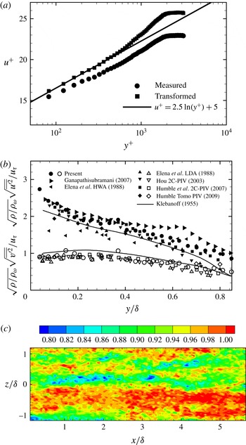
Characterization of the undisturbed boundary layer. (a) Comparison of measured and van Driest transformed velocity with logarithmic law of the wall. The transformed velocity profile in the inner variables matches with the log-law for a friction velocity
 $(u_{\unicode[STIX]{x1D70F}})=25.8~\text{m}~\text{s}^{-1}$
. ●, measured; ▪, transformed. (b) Streamwise and wall-normal velocity fluctuations within the undisturbed incoming boundary layer. Velocity fluctuations are non-dimensionalized using Morkovin’s scaling. Solid line represents the incompressible experimental data of Klebanoff (Reference Klebanoff1955) obtained at low speeds. Solid symbols represent streamwise velocity fluctuations
 $(\sqrt{\overline{u^{\prime 2}}})$
and open symbols wall-normal velocity fluctuations
 $(\sqrt{\overline{v^{\prime 2}}})$
in each case, as given in the legend. (c) Streamwise velocity (
 $u/U_{\infty }$
) contour plot in the spanwise (
 $x$
–
 $z$
) plane at
 $y/\unicode[STIX]{x1D6FF}=0.5$
(
 $y^{+}=1150$
) showing the presence of low- and high-speed streaks.

The undisturbed incoming boundary layer on the tunnel wall was measured using PIV. In order to estimate the boundary layer parameters in a supersonic boundary layer, profiles of temperature and density are also required in addition to the velocity profile. This was done following the methodology in Hou (Reference Hou2003) and Humble (Reference Humble2008) by using the Crocco–Busemann relation to obtain the temperature profile from the velocity profile, and in turn obtaining the density profile from the temperature profile. The resulting value of the boundary layer thickness was found to be close to 6 mm, while the compressible momentum thickness was found to be about 0.39 mm. Figure 2(a) shows the measured mean streamwise (●) and the corresponding transformed (▪) velocity profile obtained using the van Driest effective velocity concept in inner variables (
 $y^{+}$
). The transformed or incompressible velocity profile matched with the standard log-law for a friction velocity (
 $u_{\unicode[STIX]{x1D70F}}$
) of
 $25.8~\text{m}~\text{s}^{-1}$
. The corresponding skin-friction coefficient at the wall was
 $1.8\times 10^{-3}$
. A summary of all the main undisturbed boundary layer parameters determined is summarized in table 2. As seen from the plot, the log-law region appears to extend to
 $y^{+}\approx 700$
. The extent of the log region is smaller in our case compared to some other recent supersonic boundary layer measurements as for example of Ganapathisubramani (Reference Ganapathisubramani2007), due to the smaller values of
 $Re_{\unicode[STIX]{x1D703}}$
in our experiments.
Figure 2(b) shows the comparison of present streamwise
 $(\sqrt{\overline{u^{\prime 2}}})$
and wall-normal
 $(\sqrt{\overline{v^{\prime 2}}})$
velocity fluctuations with other experimental data from supersonic boundary layers (Elena & LaCharme Reference Elena and LaCharme1988; Hou Reference Hou2003; Ganapathisubramani Reference Ganapathisubramani2007; Humble, Scarano & Van Oudheusden Reference Humble, Scarano and Van Oudheusden2007). The streamwise and wall-normal velocity fluctuations are normalized using the friction velocity (
 $u_{\unicode[STIX]{x1D70F}}$
) and multiplied with
 $\sqrt{\unicode[STIX]{x1D70C}/\unicode[STIX]{x1D70C}_{w}}$
on account of property variations across the boundary layer in compressible flow. With this normalization, we compare our data both with recent compressible boundary layer measurements and with the incompressible results of Klebanoff (Reference Klebanoff1955). The current streamwise velocity fluctuation
 $(\sqrt{\overline{u^{\prime 2}}})$
data are within the range of values reported in other compressible boundary layer measurements, and slightly higher than the incompressible data of Klebanoff (Reference Klebanoff1955). Our wall-normal velocity fluctuations
 $(\sqrt{\overline{v^{\prime 2}}})$
again are seen to be close to other recent experimental measurements in compressible boundary layers and a little below the incompressible (Klebanoff Reference Klebanoff1955) data. It should be noted here that, as discussed by Ganapathisubramani (Reference Ganapathisubramani2007), the velocity fluctuation data measured using PIV can be affected by the interrogation box size, which essentially results in averaging of velocity over that area, and hence results in scales that are smaller than the box size not being captured. In our case, this interrogation box size (or resolution), as given in table 1 for the undisturbed boundary layer (UBL) in
 $x$
–
 $y$
plane, is approximately
 $0.08\unicode[STIX]{x1D6FF}\times 0.04\unicode[STIX]{x1D6FF}$
in
 $x$
and
 $y$
directions, respectively, which corresponds to 184 wall units by 92 wall units. Although there are some differences between the present results and prior supersonic boundary layer velocity fluctuation measurements, they are broadly consistent.
Another important characteristic of the turbulent boundary layer that has received a lot of recent attention is the presence of low- and high-speed streaks. This was measured and shown by Tomkins & Adrian (Reference Tomkins and Adrian2003) and Hutchins & Marusic (Reference Hutchins and Marusic2007) in incompressible boundary layers, and in a supersonic boundary layer by Ganapathisubramani, Clemens & Dolling (Reference Ganapathisubramani, Clemens and Dolling2006) and Humble et al. (Reference Humble, Elsinga, Scarano and Van Oudheusden2009). These structures are seen in the present measurements as well, just outside the log region (
 $y/\unicode[STIX]{x1D6FF}=0.5$
,
 $y^{+}=1150$
), as shown in figure 2(c); the low- and high-speed streaks having streamwise lengths greater than
 $6\unicode[STIX]{x1D6FF}$
and widths of approximately
 $0.5\unicode[STIX]{x1D6FF}$
, the latter being comparable to values reported in Hutchins & Marusic (Reference Hutchins and Marusic2007). In the context of SWBLI, these structures are one of the proposed reasons for low-frequency shock motions, as discussed by Ganapathisubramani et al. (Reference Ganapathisubramani, Clemens and Dolling2007), for the case of a compression ramp.
Undisturbed turbulent boundary layer properties.

2.3 Forward-facing step model
In the present study, a FFS of height (
 $h$
) equal to two times the incoming boundary layer thickness was used (
 $h/\unicode[STIX]{x1D6FF}=2$
). The model was made of aluminium and placed on the bottom wall of the test section. The spanwise width of the FFS was 60 mm and spanned the central 60 % of the test-section width of 100 mm, with a gap of 20 mm on both sides, the gap being approximately three times the boundary layer thickness. No end plates were used as it would block or obscure the field of view for PIV measurements. One concern about having no end plates is the possible effect of lateral flows. Zukoski (Reference Zukoski1967) in his review on FFS states that although small lateral flows would be present, their effects are not dominant in the central region as long as the span is five step heights or larger, which is satisfied in our case. However, in order to see if there are changes in the central region, we took PIV measurements with a larger model spanning 90 mm, which almost completely spans the test section, except for 5 mm on each side, which is close to the boundary layer thickness (6 mm). This blow-down required higher settling chamber pressures to run, and hence lower run times. The location of the centre of the separation bubble (
 $\overline{x_{c}}/h$
,
 $\overline{y_{c}}/h$
), where both
 $\overline{u}$
and
 $\overline{v}$
are zero, and the maximum reverse flow velocity (
 $\overline{u_{r,max}}/U_{\infty }$
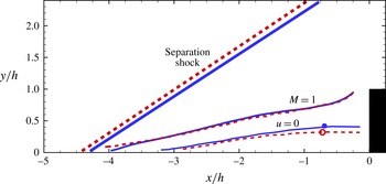
) measured from the time-averaged velocity field at the spanwise central location for the two models are shown in table 3. The important features of the time-averaged flow such as the shock location and angle, the
 $u=0$
contour and the sonic line (
 $M=1$
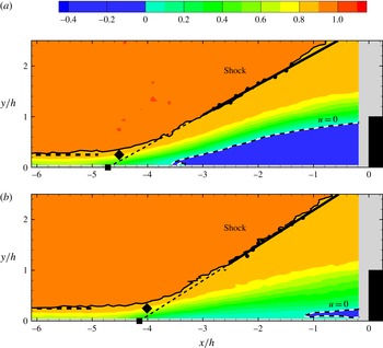
) of the two models at the spanwise central location are also directly compared in figure 3. Although there are differences, the variations are not large, indicating that the broad features of the separation bubble in the central part of the FFS model are not sensitive to the finite span length of the model. The mean shock location (
 $\overline{x_{s}}/h$
) and root-mean-square of the shock location (
 $x_{s,rms}/h$
) for the 60 mm and 90 mm span models are also shown in table 3 (the procedure for finding the shock location from wall-normal PIV measurements is described later in § 4.1). As may be seen, these are again nearly the same, showing that the mean shock location and its motions in the central region of the 60 mm span model are nearly unaffected by the finite span of the model, consistent with the statements of Zukoski (Reference Zukoski1967) for sufficiently long steps. We shall also present in the next section, PIV measurements in the spanwise (
 $x$
–
 $z$
) plane, which show that the mean flow is nearly two-dimensional across a large central span of the 60 mm model. These measurements suggest that the velocity field at the spanwise central part of the 60 mm FFS model, which is the one used throughout the rest of this study, are not sensitive to the finite span length of the model.
Comparison of the mean velocity field at the spanwise central location over the FFS for the main model having a span of 60 % of the test-section width, with a model that spans 90 % of the test-section width. The important features of the time-averaged flow such as the separation shock, the
 $u=0$
contour, the centre of the separation bubble and the sonic line (
 $M=1$
) are shown for both models. In all cases, the solid lines (blue) correspond to the 60 % span model, while the dashed lines (orange) correspond to the 90 % span model. Although there are differences, the variations are not large, indicating that the broad features of the separation bubble in the central part of the FFS model are not sensitive to the span length of the model. ●, centre of the recirculation region for the 60 % span model; ○, centre of the recirculation region for the 90 % span model.

Time-averaged recirculation region and shock location data for the FFS at the spanwise central location of the model. Data are given for the main model having a span of 60 % of the test-section width and for a model which spans 90 % of the test-section width. In the table, (
 $\overline{x_{c}}/h,\overline{y_{c}}/h$
) represents the location of the centre of the mean separation bubble,
 $\overline{u_{r,max}}/U_{\infty }$
is the normalized mean maximum reverse flow velocity,
 $\overline{x_{s}}/h$
and
 $x_{s,rms}/h$
are the mean shock location and its root-mean-square with time, respectively.

3 Time-averaged velocity field and spectra
We present in this section, time-averaged PIV velocity field measurements in two perpendicular planes, and results from long time-averaged spectra of the wall pressure fluctuations ahead of the step. All results, as stated before, are for Mach 2.54 flow over a FFS of height
 $h/\unicode[STIX]{x1D6FF}=2$
.
3.1 Mean velocity field
PIV measurements in the central wall-normal (
 $x$
–
 $y$
) plane were done both upstream and downstream of the step. The results from these measurements were processed separately and then time averaged. The time-averaged fields from both cases were then merged into a single velocity field, with the streamwise velocity (
 $\overline{u}$
) shown in figure 4(a) and the wall-normal velocity (
 $\overline{v}$
) shown in figure 4(b). As may be seen from the figure, the incoming boundary layer deflects approximately
 $4h$
upstream of the step. This location corresponds well with the separation location (
 $x_{sep}/h$
) determined from surface oil flow visualization shown in figure 5, which is approximately
 $4.1h$
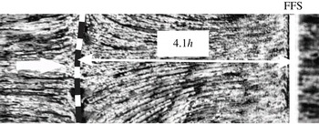
. The surface oil flow method is an established method to determine the extent of separation (Settles, Fitzpatrick & Bogdonoff Reference Settles, Fitzpatrick and Bogdonoff1979), and is implemented here by spraying oil mixed with particles on the surface ahead of the step and then imaging it after it is exposed to the flow. The image in figure 5 shows a change in surface pattern along the separation line, which is approximately constant in the spanwise direction, with small reductions away from the centre. The obtained separation location
 $x_{sep}\approx -4.1h$
is consistent with the separation location data compiled by Zukoski (Reference Zukoski1967) in his review, which show that this value is reasonably independent of step height for
 $h/\unicode[STIX]{x1D6FF}>1.2$
and also reasonably independent of Mach number over the range from approximately 2 to 4.2.
Mean velocity field over the FFS at a free-stream Mach number of 2.54 in the central wall-normal (
 $x$
–
 $y$
) plane. Contour plot of the mean streamwise velocity (
 $\overline{u}/U_{\infty }$
) is shown in (a), while the mean wall-normal velocity (
 $\overline{v}/U_{\infty }$
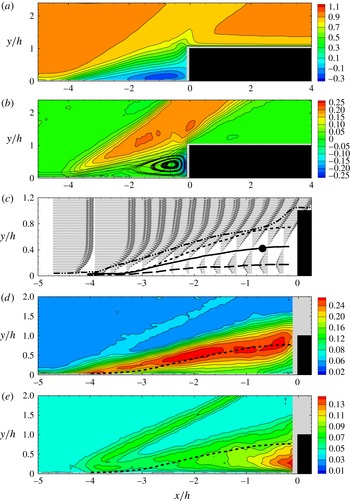
) contours are shown in (b). In both the cases, the velocity contours were obtained from two separate measurements done upstream and downstream of the step (as given in table 1) and then combined. Streamlines are also superposed in (b) to clearly show the large separation bubble formed ahead of the step. Zoomed in view of the recirculation region ahead of the step is shown in (c) along with the mean dividing streamline (small dashed line),
 $\overline{u}=0$
line (solid line), the maximum reverse velocity line (long dashed line) and the sonic line
 $(M=1)$
(dot-dashed line). Contours of the fluctuating velocity fields in the streamwise (
 $\sqrt{\overline{u^{\prime 2}}}/U_{\infty }$
) and wall-normal (
 $\sqrt{\overline{v^{\prime 2}}}/U_{\infty }$
) directions are shown in (d,e), respectively, along with the dividing streamline.

The time-averaged separation shock can be identified in figure 4(a,b) from the sharp change in flow speed and direction that is seen to occur along an approximately straight line starting from
 $x/h\approx -4$
. The flow separates at
 $x_{sep}/h\approx -4.1$
forming a large separation bubble upstream of the step, which is clearly shown by the streamlines superposed on the
 $\overline{v}$
field in (b). This separation bubble can be easily measured and seen even in the time-averaged velocity field for this geometry, unlike in compression ramp studies. This separated flow then reattaches near the step corner, where Behrens (Reference Behrens1971) suggests that there is a bow shock followed by a series of expansion waves, the latter responsible for turning the flow and making it parallel to the lower wall again. The bump in the mean streamwise velocity (
 $\overline{u}$
) contours seen near the top step corner, also seen by Behrens (Reference Behrens1971), is likely related to the existence of a bow shock near the corner. Ahead of the separation bubble, at the separation shock, the streamlines are found to deflect by approximately
 $13^{\circ }$
forming a virtual ramp, which is broadly consistent with the mean flow picture ahead of the step discussed for example in the review of Zukoski (Reference Zukoski1967). Compared to the compression ramp cases, the separation bubble formed ahead of the step is much larger, as expected, and hence easier to resolve with PIV measurements, as seen from the zoomed in view of the velocity field shown in figure 4(c). In this plot, we show the mean streamwise velocity (
 $\overline{u}$
) profiles at different streamwise locations (
 $x$
), which clearly show the reverse flow within the separated region. Also shown in the figure is the
 $\overline{u}=0$
line (solid line) that demarcates the reverse flow region (
 $\overline{u}<0$
), the maximum reverse flow line (long dashed line), the dividing streamline (short dashed line) and the sonic line
 $(M=1)$
(dot-dashed line). The dividing streamline here is defined as the set of points
 $y_{j}(x)$
, where
 $\int _{0}^{y_{j}(x)}\overline{u}\,\text{d}y=0$
, as in Piponniau et al. (Reference Piponniau, Dussauge, Debiève and Dupont2009), the assumption being that density variations within the relatively low-speed recirculation region are neglected. The maximum time-averaged reverse velocity (
 $\overline{u_{r,max}}/U_{\infty }$
) within the separation bubble is found to be approximately 0.23 of the free-stream velocity, with the centre of the separation bubble occurring at
 $\overline{x_{c}}/h=-0.69$
and
 $\overline{y_{c}}/h=0.42$
. We also present in figure 4(d,e) the streamwise (
 $\sqrt{\overline{u^{\prime 2}}}$
) and wall-normal (
 $\sqrt{\overline{u^{\prime 2}}}$
) velocity fluctuations. The largest values of (
 $\sqrt{\overline{u^{\prime 2}}}/U_{\infty }$
) are found to occur around the mean dividing streamline, also shown in the plot, with peak values of approximately 0.25. On the other hand, the maximum values of (
 $\sqrt{\overline{v^{\prime 2}}}/U_{\infty }$
) are found to occur closer to the vertical step face with a maximum value of approximately 0.14. The location of the separation shock can also be clearly seen from the contours, due to the velocity changes induced by the oscillating separation shock.
Surface oil flow visualization ahead of the FFS showing the mean separation line. The picture shows the top view visualization with flow from left to right. The field of view in the spanwise direction (
 $z$
) is approximately
 $2h$
and FFS represents the location of the forward-facing step.

Apart from the wall-normal (
 $x$
–
 $y$
) plane, PIV measurements were also done in the spanwise (
 $x$
–
 $z$
) plane at various wall-normal (
 $y$
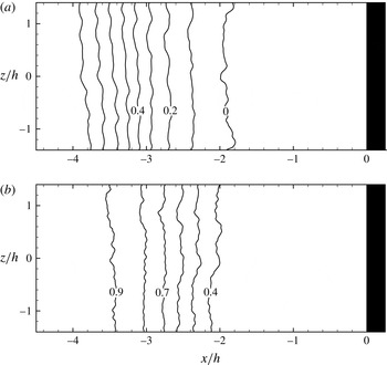
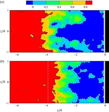
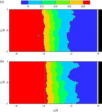
) locations. The mean streamwise velocity contour plot at two wall-normal locations,
 $y/h=0.25$
and 0.50, are shown in figure 6. At both wall-normal locations, the mean streamwise velocity (
 $\overline{u}$
) contour lines are found to be nearly parallel to the step face indicating that the time-averaged flow is nearly two-dimensional over the central
 $2.8h$
of the FFS model shown, this representing approximately 50 % of the total span of the model (
 $5h$
). This is also consistent with the earlier results from the surface oil flow visualization.
3.2 Spectra of wall pressure fluctuations
The wall pressure fluctuations were measured with Kulite pressure transducers at two locations ahead of the step. Details of the transducers used are discussed in § 2.1. The two locations where the measurements were made are at the approximate location of the separation point (
 $x/h=-4.2$
) and in the middle of the separation bubble ahead of the step (
 $x/h=-2.1$
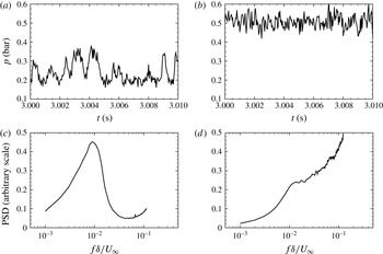
). Typical time traces of the wall pressure fluctuations at the two locations are shown in figure 7(a,b). As may be seen, the time series data in (a) at the approximate separation point (
 $x/h=-4.2$
), clearly show the presence of low-frequency oscillations in addition to high-frequency fluctuations. This is in contrast to the time series in (b) corresponding to
 $x/h=-2.1$
, where the low-frequency oscillations are absent and only the high-frequency fluctuations are seen. The frequency content of the fluctuations can be more clearly seen from the power spectral density of the pressure signal obtained using the method given in Priebe & Martin (Reference Priebe and Martin2012). This is done using Welch’s method for spectral estimation with 50 % overlap and a Hamming window for weighting the data prior to fast Fourier transform processing. Figure 7(c,d) show the premultiplied power spectral density of the wall pressure signal at two streamwise locations,
 $x/h=-4.2$
and
 $x/h=-2.1$
, respectively. The spectra corresponding to
 $x/h=-4.2$
clearly shows a low-frequency peak at
 $f\unicode[STIX]{x1D6FF}/U_{\infty }\approx 0.01$
, which is two orders of magnitude below the characteristic frequency of the incoming boundary layer. This peak thus clearly corresponds to the low-frequency motions of the shock that has received lot of recent attention (Clemens & Narayanaswamy Reference Clemens and Narayanaswamy2014). On the other hand, there is no clear low-frequency peak at
 $x/h=-2.1$
within the separation bubble, although there is a small hint of a plateau at
 $f\unicode[STIX]{x1D6FF}/U_{\infty }\approx 0.01$
, consistent with the measurements for example of Erengil & Dolling (Reference Erengil and Dolling1991) for a compression ramp. In the context of FFS, the existence of low-frequency shock oscillations at about the mean shock location has been reported earlier by Kistler (Reference Kistler1964) and Behrens (Reference Behrens1971).
Mean streamwise velocity (
 $\overline{u}/U_{\infty }$
) contours in the spanwise (
 $x$
–
 $z$
) plane at wall-normal locations of (a)
 $y/h=0.25$
and (b)
 $y/h=0.50$
. Flow is from left to right and the step is shown on the right in black.

Apart from the boundary layer scale, another method of normalizing the low-frequency motions, as suggested by Dussauge, Dupont & Debiève (Reference Dussauge, Dupont and Debiève2006), is using
 $St_{L}=fL/U_{\infty }$
, where
 $L$
is the streamwise length of the separation bubble. In our case, given that
 $L\approx 4.1h$
,
 $St_{L}=fL/U_{\infty }\approx 0.08$
, which is somewhat higher than the range suggested in Dussauge et al. (Reference Dussauge, Dupont and Debiève2006). However, if we use the definition of
 $L$
as being the intermittent region (Piponniau et al.
Reference Piponniau, Dussauge, Debiève and Dupont2009; Clemens & Narayanaswamy Reference Clemens and Narayanaswamy2014), which our measurements in the next section show is of the order of
 $h$
, then
 $St_{L}\approx 0.02$
, which is broadly in agreement with the range suggested in Piponniau et al. (Reference Piponniau, Dussauge, Debiève and Dupont2009) and Clemens & Narayanaswamy (Reference Clemens and Narayanaswamy2014).
Time traces and spectra of the wall pressure fluctuations at two locations upstream of the step. The time trace and spectra of the wall pressure at
 $x/h=-4.2$
, close to the mean separation location, is shown in (a,c), respectively, while the time trace and spectra corresponding to
 $x/h=-2.1$
, within the separation bubble, are shown in (b) and spectra (d), respectively.

In summary, the mean velocity field in the central wall-normal (
 $x$
–
 $y$
) plane shows that the incoming boundary layer separates upstream of the step forming a large separation bubble ahead of the step. Due to its large size in the wall-normal (
 $y$
) direction, this separation bubble can be relatively well resolved in measurements compared to the compression ramp cases. Surface oil flow visualization shows that the separation occurs at
 $4.1h$
upstream of the step. The oil flow visualization and the mean streamwise (
 $\overline{u}/U_{\infty }$
) velocity contours in the spanwise (
 $x$
–
 $z$
) plane at various wall-normal (
 $y$
) locations show that the contours are nearly parallel to the step, indicating that the flow is reasonably two-dimensional in the time-averaged sense.
Wall pressure fluctuation spectra close to the separation location show a dominant frequency that is two orders of magnitude smaller than the characteristic frequency present in the incoming boundary layer (
 $U_{\infty }/\unicode[STIX]{x1D6FF}$
). This peak thus clearly corresponds to the low-frequency motions of the shock that have received lot of recent attention (Clemens & Narayanaswamy Reference Clemens and Narayanaswamy2014).
4 PIV – cross-stream view
We now proceed to present results from instantaneous PIV fields in the cross-stream or wall-normal (
 $x$
–
 $y$
) plane. As one might expect, there are large variations with time of the separation shock location and the separation bubble, and we shall first show and quantify these variations. An important point related to these variations, is the recently debated question of the source of the low-frequency shock motions in shock wave–boundary layer interactions. The present geometry permits clear measurements of the separation bubble and therefore can potentially help this debate. With this is mind, we extract from each one of a large set of instantaneous fields, the shock location, a quantity representative of structures in the upstream boundary layer, and a quantity representative of the downstream separation bubble. With respect to the separation shock, we consistently make a difference between the shock foot (location denoted as
 $x_{sf}$
) measured within the boundary layer, and the main shock (location denoted as
 $x_{s}$
), which is defined and measured outside the boundary layer and separation bubble, as done for example in the simulations of Priebe & Martin (Reference Priebe and Martin2012). We shall first present measurements from instantaneous fields in § 4.1, followed by presentation of conditionally averaged fields (in § 4.2), and then a discussion of correlation coefficients (§ 4.3) to look at the relative importance of upstream and downstream effects on the shock motions.
4.1 Instantaneous
We will start with defining the various parameters of interest and then extract these quantities from instantaneous PIV velocity fields in the central wall-normal (
 $x$
–
 $y$
) plane. The separation shock location is in general a function of both the wall-normal coordinate (
 $y$
) and time, as discussed for example in Wu & Martin (Reference Wu and Martin2008). In the present work, we define, in particular, the shock at two vertical locations, one well outside the boundary layer and separation bubble, which we refer to as the main separation shock location
 $x_{s}$
, and another within the boundary layer, which we refer to as the shock foot location
 $x_{sf}$
.
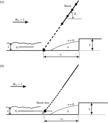
The separation shock location (
 $x_{s}$
) is determined here by locating the streamwise points far from the wall (
 $y/h=1.5$
–2.1) where the flow is deflected by greater than
 $6.5^{\circ }$
; this threshold deflection criterion being half the deflection angle of the mean flow. This is schematically shown in figure 8(a) with the located points at each wall-normal (
 $y$
) location being indicated by a solid circle. A straight line is fitted through these solid circles using least squares method (marked as a solid line) and is extended up to the wall (shown by the dotted line) to locate the separation shock location (
 $x_{s}$
).
(a) Schematic showing the methodology for extraction of instantaneous shock location (
 $x_{s}$
) from velocity data well outside the boundary layer. Shock location at a particular wall-normal location (
 $y$
) is found by locating the streamwise (
 $x$
) position where the flow is deflected as represented by the solid circle (●). A straight line is fitted through these solid circles using least squares method (solid line); this being extended to the wall (dotted line) to locate the separation shock location,
 $x_{s}$
(▪). The angle formed by the shock with the horizontal is represented as
 $\unicode[STIX]{x1D6FD}_{s}$
. The area (
 $A$
) enclosed by the zero streamwise velocity contour (
 $u=0$
) is taken as a measure of the reverse flow region, and
 $u_{l}^{\prime }$
is the line-averaged boundary layer velocity fluctuation. (b) Schematic representation illustrating the methodology used to locate the shock foot,
 $x_{sf}$
(♦) from velocity data within the boundary layer. The shock foot location (
 $x_{sf}$
) is found by locating the streamwise (
 $x$
) position where the streamwise velocity crosses a threshold value of
 $0.8U_{\infty }$
at a wall-normal (
 $y$
) location within the boundary layer at
 $y/h=0.25$
(or
 $y/\unicode[STIX]{x1D6FF}=0.5$
).

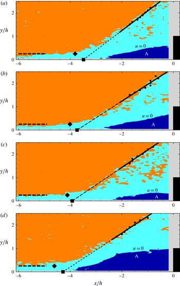
Examples of instantaneous velocity fields in the wall-normal (
 $x$
–
 $y$
) plane showing the instantaneous shock location (
 $x_{s}$
, ▪) and the shock foot location (
 $x_{sf}$
, ♦), as defined in figure 8. In the figure, orange represents the free stream with
 $u>0.9U_{\infty }$
, dark blue represents the recirculation area (
 $A$
) with
 $u<0$
, and the light blue represents the region with intermediate velocities
 $0.9U_{\infty }<u<0$
. In each case, the shock outside the boundary layer is determined using the methodology shown in figure 8(a) with the solid straight line representing the shock, and this line being extended to the wall (dotted line) to locate the separation shock location,
 $x_{s}$
(▪). The horizontal dashed line represents the location of line-averaged velocity.

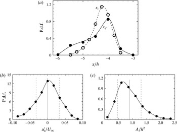
Probability density functions (p.d.f.s) of (a) shock location (
 $x_{s}/h$
) and shock foot location (
 $x_{sf}/h$
), (b) the line-averaged boundary layer velocity (
 $u_{l}^{\prime }/U_{\infty }$
) and (c) the recirculation area (
 $A/h^{2}$
). These statistics were obtained from a set of instantaneous cross-stream (
 $x$
–
 $y$
) plane velocity fields as shown in figure 9. In (a), the open symbols and dashed line show the p.d.f. of the shock (
 $x_{s}$
), while the filled symbols and solid line show the p.d.f. of the shock foot (
 $x_{sf}$
). In (b,c), the solid vertical line shows the mean value (
 $\unicode[STIX]{x1D707}$
) and the dashed vertical lines on either side show the variation by one standard deviation (
 $\unicode[STIX]{x1D70E}$
).

In contrast to the definition of
 $x_{s}$
, we also define a shock foot location (
 $x_{sf}$
) based on the velocity data within the boundary layer. The shock foot location (
 $x_{sf}$
) is found by locating the streamwise (
 $x$
) position where the streamwise velocity reduces below a threshold value at a wall-normal location within the boundary layer. This type of criterion has been used to locate a surrogate separation point in the spanwise PIV study of Ganapathisubramani et al. (Reference Ganapathisubramani, Clemens and Dolling2009). In particular, we use for this a wall-normal location of
 $y/\unicode[STIX]{x1D6FF}=0.5$
(or
 $y/h=0.25$
), as schematically illustrated in figure 8(b). We use a threshold of 80 % of the free-stream velocity to identify the location of the shock foot; this being found to be the most suitable in locating the shock foot without being affected by fluctuations present within the boundary layer. This threshold of 80 % of free-stream velocity is approximately three standard deviations below the mean undisturbed boundary layer velocity at this height within the boundary layer, the standard deviation representing the streamwise velocity fluctuations in the undisturbed upstream boundary layer at this height. This same threshold is also used later in our spanwise PIV measurements.
From each instantaneous field, we also extract a quantity to represent the upstream effect from structures in the boundary layer. For this, we compute a line-averaged streamwise velocity fluctuation (
 $u_{l}^{\prime }$
), between
 $x/h$
of
 $-6$
and
 $-5$
at
 $y/h=0.25$
(or
 $y/\unicode[STIX]{x1D6FF}=0.5$
) within the boundary layer, as shown schematically in figure 8(a,b). This type of quantity has been used by Ganapathisubramani et al. (Reference Ganapathisubramani, Clemens and Dolling2007, Reference Ganapathisubramani, Clemens and Dolling2009) to locate the presence of low- and high-speed streaks in the incoming boundary layer, which can influence the shock motions.
On the downstream side, the area of the reverse flow (
 $u<0$
) region denoted as
 $A$
can be extracted from each field, as illustrated in figure 8. This type of parameter has previously been used by Wu & Martin (Reference Wu and Martin2008) to determine correlation of the shock position with the downstream separation bubble in their simulations of SWBLI in flow over a compression ramp, and also by Pearson et al. (Reference Pearson, Goulart and Ganapathisubramani2013) in their experimental study of subsonic flow over a FFS.
A few example cases of instantaneous velocity fields is shown in figure 9. In each plot, important parameters such as the shock location (
 $x_{s}$
, ▪), shock foot location (
 $x_{sf}$
, ♦) and the recirculation region area (
 $A$
) enclosed by the
 $u=0$
contour are also marked. The
 $u=0.9U_{\infty }$
contour is also shown in each case, which gives an idea of both the instantaneous boundary layer thickness and the approximate location of the shock in the region outside the boundary layer. It is clear from these example cases that the shock location (
 $x_{s}$
), the shock foot location (
 $x_{sf}$
), the thickness of the incoming boundary layer and the recirculation region area (
 $A$
) can all vary substantially at different instants in time.
The variation of the flow and shock parameters with time can be seen more clearly in figure 10, where the variation of all important parameters extracted from each of the 800 instantaneous fields is shown in the form of probability density functions (p.d.f.s). It is clear that all parameters vary significantly with time, with some of the parameters such as the shock foot location (
 $x_{sf}$
) and the recirculation area (
 $A$
) showing a clearly skewed p.d.f. The superimposed p.d.f. of the shock and shock foot (in a) clearly shows the larger variability of the shock foot compared to the shock, and also contrasts the reasonably symmetric nature of the shock (
 $x_{s}$
) p.d.f. with the significantly asymmetric one for the shock foot (
 $x_{sf}$
). The recirculation area (
 $A$
) p.d.f. has a peak at approximately
 $0.65h^{2}$
, which is quite large compared to the subsonic FFS case in Pearson et al. (Reference Pearson, Goulart and Ganapathisubramani2013) where the peak of the p.d.f. occurs at approximately
 $0.05h^{2}$
. In general, the recirculation area (
 $A$
) in the present case is much larger, a consequence of the fact that the separation occurs much further upstream compared to the subsonic case. In figure 10(b,c), we show the corresponding mean value (
 $\unicode[STIX]{x1D707}$
) by a solid vertical line and one standard deviation (
 $\unicode[STIX]{x1D70E}$
) on either side by vertical dashed lines.
4.2 Conditionally averaged fields
We present in this subsection conditionally averaged velocity fields; the conditions being based on either the incoming boundary layer velocity fluctuation (
 $u_{l}^{\prime }$
) or the downstream recirculation region area (
 $A$
). This should give an idea of the importance of either of these parameters on the shock location, as discussed for example in Ganapathisubramani et al. (Reference Ganapathisubramani, Clemens and Dolling2007) based on a surrogate separation location and Piponniau et al. (Reference Piponniau, Dussauge, Debiève and Dupont2009) based on the separation bubble size.
4.2.1 Incoming boundary layer velocity fluctuation (
 $u_{l}^{\prime }$
)

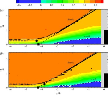
Conditionally averaged streamwise (
 $u/U_{\infty }$
) velocity field based on line-averaged streamwise velocity fluctuations (
 $u_{l}^{\prime }$
) in the incoming boundary layer. (a) Negative velocity fluctuations between (
 $\unicode[STIX]{x1D707}-2\unicode[STIX]{x1D70E}$
) and (
 $\unicode[STIX]{x1D707}-2.5\unicode[STIX]{x1D70E}$
). (b) Positive velocity fluctuations between (
 $\unicode[STIX]{x1D707}+2\unicode[STIX]{x1D70E}$
) and (
 $\unicode[STIX]{x1D707}+2.5\unicode[STIX]{x1D70E}$
), where
 $\unicode[STIX]{x1D707}$
and
 $\unicode[STIX]{x1D70E}$
are the mean and standard deviation of the line-averaged streamwise velocity fluctuations (
 $u_{l}^{\prime }$
) in the incoming boundary layer, respectively. The shock location and the recirculation region (
 $u=0$
contour) are also highlighted. ▪, shock location (
 $x_{s}$
); ♦, shock foot location (
 $x_{sf}$
); - - -, line from which boundary layer velocity (
 $u_{l}^{\prime }$
) is extracted.

Conditional averaging to determine the relation between the shock foot and the upstream boundary layer fluctuations have been done previously for example by Beresh et al. (Reference Beresh, Clemens and Dolling2002) and Ganapathisubramani et al. (Reference Ganapathisubramani, Clemens and Dolling2007) in the case of a compression ramp. In the present case of the FFS, we obtain conditionally averaged fields based on the line-averaged streamwise velocity fluctuations (
 $u_{l}^{\prime }$
) in the incoming boundary layer. This parameter should pick up low- and high-speed streaks present in turbulent boundary layers, as discussed by Ganapathisubramani et al. (Reference Ganapathisubramani, Clemens and Dolling2007). As shown in figure 10(b),
 $u_{l}^{\prime }/U_{\infty }$
has a standard deviation (
 $\unicode[STIX]{x1D70E}$
) of approximately 3.3 % at
 $y/\unicode[STIX]{x1D6FF}=0.5$
. For conditional averaging based on positive streamwise velocity fluctuation (
 $+u_{l}^{\prime }$
), we use PIV velocity fields which have streamwise velocity fluctuations between (
 $+2\unicode[STIX]{x1D70E}$
) and (
 $+2.5\unicode[STIX]{x1D70E}$
). Similarly for conditional averaging based on negative streamwise velocity fluctuations (
 $-u_{l}^{\prime }$
), PIV velocity fields which have streamwise velocity fluctuations between (
 $-2\unicode[STIX]{x1D70E}$
) and (
 $-2.5\unicode[STIX]{x1D70E}$
) have been used. It may be noted that this condition was chosen as a balance between having events that are sufficiently away from the mean (in
 $+$
and
 $-$
), while still having sufficient number of events with the chosen condition. Figure 11(a,b) shows conditionally averaged velocity field based on the negative (
 $-u_{l}^{\prime }$
) and positive (
 $+u_{l}^{\prime }$
) streamwise velocity fluctuations in the incoming boundary layer, respectively. As may be expected, this conditional average results in clear differences in the upstream boundary layer thickness in the two cases, with the (
 $-u_{l}^{\prime }$
) case in (a) having a significantly thicker boundary layer than the (
 $+u_{l}^{\prime }$
) case in (b). In both cases, the separation shock location (
 $x_{s}$
, ▪) determined from the velocity field outside the boundary layer, and the shock foot (
 $x_{sf}$
, ♦) based on velocity data within the boundary layer are also indicated. The figure shows that the separation shock location (
 $x_{s}$
) is approximately
 $4.2h$
upstream of the step in both cases. It may be noted that the number of PIV velocity fields for conditional averaging based on positive streamwise velocity fluctuations (
 $+u_{l}^{\prime }$
) was eleven and for negative (
 $-u_{l}^{\prime }$
) was eighteen. Although the number of realizations are not large, we found that the shock location remained close to
 $-4.2h$
in both the cases even with half the realizations, suggesting that the results are reasonably robust. The nearly identical shock location (
 $x_{s}$
) for the (
 $-u_{l}^{\prime }$
) and (
 $+u_{l}^{\prime }$
) cases implies that the separation shock location is not strongly correlated to the incoming boundary layer streamwise velocity fluctuations. This result appears at first to differ from the results of some studies on compression ramps such as those of Unalmis & Dolling (Reference Unalmis and Dolling1998), Andreopoulos, Agui & Briassulis (Reference Andreopoulos, Agui and Briassulis2000), Beresh et al. (Reference Beresh, Clemens and Dolling2002) and Ganapathisubramani et al. (Reference Ganapathisubramani, Clemens and Dolling2007). However, this is not necessarily the case. In these earlier studies, the shock foot close to the lower wall was measured either from PIV or wall pressure fluctuations, and not necessarily the separation shock which is present a little further away from the wall. This can be seen from the shock foot location (
 $x_{sf}$
) measured within the boundary layer, which shows significant differences in the two cases, with values of about
 $-4.3h$
and
 $-3.8h$
corresponding to the (
 $-u_{l}^{\prime }$
) and (
 $+u_{l}^{\prime }$
) condition, respectively. This suggests that the shock foot is more responsive to the boundary layer fluctuations consistent with the observations of Priebe & Martin (Reference Priebe and Martin2012) in the case of the compression ramp. In contrast, the main separation shock measured well outside the boundary layer remains nearly unaffected by these fluctuations.
4.2.2 Separation bubble or recirculation region area (
$A$
)

Conditionally averaged streamwise velocity field (
 $u/U_{\infty }$
) based on recirculation region area (
 $A$
). (a) Big recirculation area between (
 $\unicode[STIX]{x1D707}+2\unicode[STIX]{x1D70E}$
) and (
 $\unicode[STIX]{x1D707}+2.5\unicode[STIX]{x1D70E}$
). (b) Small recirculation area between (
 $\unicode[STIX]{x1D707}-1.5\unicode[STIX]{x1D70E}$
) and (
 $\unicode[STIX]{x1D707}-2\unicode[STIX]{x1D70E}$
) where
 $\unicode[STIX]{x1D707}$
and
 $\unicode[STIX]{x1D70E}$
are the mean and standard deviation of the recirculation region area, respectively. The shock location and the recirculation region (
 $u=0$
contour) are also highlighted. ▪, shock location (
 $x_{s}$
); ♦, shock foot location (
 $x_{sf}$
); - - -, line from which boundary layer velocity (
 $u_{l}^{\prime }$
) is extracted.

The effect of the downstream parameter on the separation shock location is discussed here using conditional averaging based on the separation bubble or recirculation area (
 $A$
). As shown in figure 10(c), the normalized recirculation area (
 $A/h^{2}$
) varies between 0 and 2.4. The mean (
 $\unicode[STIX]{x1D707}$
) and standard deviation (
 $\unicode[STIX]{x1D70E}$
) of its variation is 0.9 and 0.4, respectively. For conditional averaging based on larger separation bubble, velocity fields which have bubble area between (
 $\unicode[STIX]{x1D707}+2\unicode[STIX]{x1D70E}$
) and (
 $\unicode[STIX]{x1D707}+2.5\unicode[STIX]{x1D70E}$
) were used, while for conditional averaging based on smaller separation bubble, velocity fields which have bubble area between (
 $\unicode[STIX]{x1D707}-1.5\unicode[STIX]{x1D70E}$
) and (
 $\unicode[STIX]{x1D707}-2\unicode[STIX]{x1D70E}$
) were used. It may be noted here that the differences in the choice of the two ranges for conditional averaging based on the separation bubble size (
 $A$
) was necessitated by the asymmetry in the p.d.f. of the recirculation region about its mean value as seen in figure 10(c). Figure 12(a,b) shows conditionally averaged velocity field based on larger and smaller separation bubble, respectively. As may be seen there is a significant difference in the separation shock location
 $x_{s}$
between the two conditions, with values of approximately
 $4.8h$
and
 $4.2h$
upstream of the step for the larger and smaller separation bubble, respectively. It may be noted that the number of PIV velocity fields for conditional averaging based on large separation bubble area was 15 and for small separation bubble area was 23. Although the number of realizations are not large, we found that the shock location even with half the realizations was within
 $0.1h$
of the above mentioned values, indicating that the condition appears to be strong enough to give a robust result even with this smaller number of realizations. The significant difference in shock location between the large separation bubble and the small separation bubble suggests that the separation shock location is reasonably correlated to the separation bubble area. This result is similar to the observation of Piponniau et al. (Reference Piponniau, Dussauge, Debiève and Dupont2009), who show that the shock location is significantly affected when the velocity fields are conditioned based on the separation bubble size for the case of an impinging–reflecting shock. Further, in our case, it may also be noted that the shock foot location (
 $x_{sf}$
) shifts along with the
 $x_{s}$
location, and its corresponding values are
 $-4.5h$
and
 $-4h$
, respectively, both being approximately
 $0.2h$
downstream from the
 $x_{s}$
location. This suggests that the separation bubble size is correlated to both the shock and the shock foot. On the other hand, the conditional fields based on the low- and high-speed streaks in the boundary layer show significant changes only for the shock foot location, suggesting that the correlations are significant only between the shock foot and the boundary layer fluctuations. We shall see this further from correlation measurements in the next subsection, and from the spanwise PIV fields in the next section.
4.3 Correlation coefficient
To understand the importance of upstream and downstream parameters, we calculate correlation coefficients of both the shock location (
 $x_{s}$
) and the shock foot location (
 $x_{sf}$
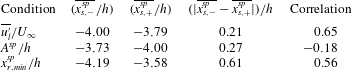
) with these parameters from the set of about 800 instantaneous cross-stream PIV fields. Table 4 shows the correlation coefficient of both the separation shock (
 $x_{s}/h$
) and the shock foot location (
 $x_{sf}/h$
) with the upstream line-averaged streamwise velocity fluctuation (
 $u_{l}^{\prime }/U_{\infty }$
) and the downstream separation bubble area (
 $A/h^{2}$
).
The correlation coefficient between separation shock location (
 $x_{s}/h$
) and upstream line-averaged streamwise velocity fluctuations (
 $u_{l}^{\prime }/U_{\infty }$
) is found to be
 $-0.03$
. This shows that there is very weak correlation between the upstream incoming boundary layer and the separation shock location based on the shock outside the boundary layer. On the other hand, the correlation coefficient between the separation shock location (
 $x_{s}/h$
) and the downstream separation bubble area (
 $A/h^{2}$
) is found to be
 $-0.26$
, which shows that there is a significant correlation of the shock motions with separation bubble or downstream parameter. This type of weak correlation of shock motion with the incoming boundary layer fluctuation, and a stronger correlation to the downstream separation bubble, has also been reported by Wu & Martin (Reference Wu and Martin2008) and Piponniau et al. (Reference Piponniau, Dussauge, Debiève and Dupont2009). It may be noted that the robustness/uncertainty of the correlation values was checked by calculating these values with half of the total of 800 realizations. The results were found to be varying by less than 0.03 indicating robustness of the correlation values and the above conclusion.
Apart from the main separation shock location (
 $x_{s}/h$
) that is based on the shock outside the boundary layer, we have also extracted the shock foot location (
 $x_{sf}/h$
) based on velocity data within the boundary layer. The correlation coefficients calculated for shock foot location (
 $x_{sf}$
) with the upstream and downstream influencing parameters is also given in table 4. The correlation coefficient between the separation shock foot location (
 $x_{sf}/h$
) and the upstream parameter (
 $u_{l}^{\prime }/U_{\infty }$
) is found to be 0.55, which is quite significant. This suggests that the shock foot is well correlated with the upstream parameter that is linked to the structures within the boundary layer, as discussed by Ganapathisubramani et al. (Reference Ganapathisubramani, Clemens and Dolling2007). The value of the correlation coefficient is also comparable to the value of 0.4 reported by Ganapathisubramani et al. (Reference Ganapathisubramani, Clemens and Dolling2007) and of approximately 0.5 reported by Wu & Martin (Reference Wu and Martin2008). The correlation coefficient between shock foot location (
 $x_{sf}/h$
) and the downstream parameter (
 $A/h^{2}$
) is found to be
 $-0.27$
, which is less than that with the upstream parameter, but still significant. This is consistent with the results from the conditionally averaged fields based on the separation bubble that showed significant changes in both the location of the main shock outside the boundary layer (
 $x_{s}$
) and the shock foot (
 $x_{sf}$
) within the boundary layer. This is also supported by the fact that the correlation coefficient for both the shock and the shock foot with the recirculation area are nearly the same,
 $-0.26$
and
 $-0.27$
, respectively, as shown in table 4. To further emphasize this point, we also present in the table correlation coefficients between
 $(x_{sf}-x_{s})/h$
with both
 $u_{l}^{\prime }/U_{\infty }$
and
 $A/h^{2}$
, with the corresponding values being 0.65 and 0.02, respectively. Clearly, the difference between
 $(x_{sf}-x_{s})/h$
is highly correlated to
 $u_{l}^{\prime }/U_{\infty }$
and not at all to
 $A/h^{2}$
. The difference between the two shock locations is in effect a measure of the spanwise ripple or wrinkling of the shock, which is well correlated only to the fluctuations in the boundary layer (
 $u_{l}^{\prime }$
). As discussed by Ganapathisubramani et al. (Reference Ganapathisubramani, Clemens and Dolling2007), the structures in the boundary layer that cause these effects are likely to be the long coherent regions of streamwise velocity fluctuations that have been shown by many researchers (Tomkins & Adrian Reference Tomkins and Adrian2003; Hutchins & Marusic Reference Hutchins and Marusic2007). We shall discuss this point further in the next section. It should be noted here that all correlation coefficients presented here and in the following section are values calculated at the same time instant. As shown by Wu & Martin (Reference Wu and Martin2008) and Ganapathisubramani et al. (Reference Ganapathisubramani, Clemens and Dolling2009), the correlation coefficients will be higher if a time lag, of the order of approximately
 $7\unicode[STIX]{x1D6FF}/U_{\infty }$
is used, corresponding to the time taken for example of an upstream structure in the boundary layer to affect the shock position. The values obtained at the same instant, corresponding to zero time lag, are however quite indicative as shown by the same two studies.
Hence, the correlation coefficient values in the wall-normal (
 $x$
–
 $y$
) plane suggest that the boundary layer structures influence the shock foot (
 $x_{sf}$
). In contrast, the main shock location outside the boundary layer (
 $x_{s}$
) is not well correlated to the boundary layer structures, but is instead reasonably well correlated to the downstream recirculation region area (
 $A$
). The downstream influence being more important in the present FFS case is consistent with the statements of Priebe & Martin (Reference Priebe and Martin2012) and Clemens & Narayanaswamy (Reference Clemens and Narayanaswamy2014), who state that downstream influences are likely to be more important in strongly separated cases. We shall further expand on this point in the next section, as we present PIV results in the spanwise (
 $x$
–
 $z$
) plane.
Correlation coefficient of shock (
 $x_{s}$
) and shock foot (
 $x_{sf}$
) location with boundary layer velocity (
 $u_{l}^{\prime }$
) and recirculation region area (
 $A$
) in the central cross-stream (
 $x$
–
 $y$
) plane.

5 PIV – spanwise view
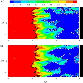
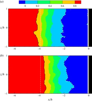
Two sample instantaneous streamwise velocity (
 $u/U_{\infty }$
) contour plots in the spanwise (
 $x$
–
 $z$
) plane at
 $y/h=0.25$
. In the figure, the white dashed line represents the
 $u=0$
contour or the recirculation line (
 $x_{r}^{sp}$
) and the black continuous line represents the
 $u=0.8U_{\infty }$
condition that represents the shock location (
 $x_{s}^{sp}$
).

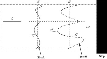
Schematic of the spanwise view of the FFS showing the shock location (
 $x_{s}^{sp}$
) and the recirculation line (
 $x_{r}^{sp}$
) that represents the
 $u=0$
condition. Both these parameters vary with spanwise location as illustrated in the figure. The area of the recirculation region with
 $u<0$
per unit span in this spanwise (
 $x$
–
 $z$
) plane is denoted as
 $A^{sp}$
.

In the previous section, we presented results from velocity field measurements in the wall-normal (
 $x$
–
 $y$
) plane. In this section, we present results from PIV measurements in the spanwise (
 $x$
–
 $z$
) plane, as in the study of Ganapathisubramani et al. (Reference Ganapathisubramani, Clemens and Dolling2007, Reference Ganapathisubramani, Clemens and Dolling2009) for the case of a compression ramp.
5.1 Instantaneous
Two example instantaneous streamwise velocity (
 $u/U_{\infty }$
) contour plots in the spanwise plane at
 $y/h=0.25$
(or
 $y/\unicode[STIX]{x1D6FF}=0.5$
) are shown in figure 13. Apart from the general contours of streamwise velocity, two particular contour levels, namely, the
 $u=0$
contour and the
 $u=0.8U_{\infty }$
contours are highlighted. The
 $u=0$
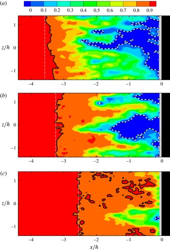
contour, shown by the white dashed line, demarcates the reverse velocity region, and may be used to gain an idea of the recirculation region, as in the previous section. It is clear from the two examples shown in the figure that this recirculation region has very large spanwise variations of approximately
 $3h$
in the instantaneous fields. The other contour that is marked in the figure is the
 $u=0.8U_{\infty }$
contour, shown by a thick black line, which may be used as a surrogate for determining the shock foot, as discussed in the previous section, and similar to the criterion used by Ganapathisubramani et al. (Reference Ganapathisubramani, Clemens and Dolling2007). As seen in the two example cases, this contour line representing the shock foot has variations in the spanwise direction, but these are relatively small, at approximately
 $0.5h$
, compared to the very large variations (approximately
 $3h$
) seen in the
 $u=0$
contour line. The observed spanwise variations in the shock may be interpreted as the spanwise ripples or wrinkling of the shock foot about the mean shock foot line, as discussed by Wu & Martin (Reference Wu and Martin2008), Ganapathisubramani et al. (Reference Ganapathisubramani, Clemens and Dolling2009) and Priebe & Martin (Reference Priebe and Martin2012).
From instantaneous spanwise velocity fields, as in figure 13, we can extract many parameters related to the shock location, the extent of the recirculation or reverse flow region and the incoming boundary layer velocity fluctuations. These are schematically shown in figure 14. In the figure, the line-averaged streamwise velocity fluctuation is represented as
 $u_{l}^{\prime }$
, as in the previous section, and in this case is a function of the spanwise
 $z$
location. We can also obtain the shock location from a threshold streamwise velocity criterion, as in the previous section, and we denote this as
 $x_{s}^{sp}$
, which is again clearly dependent on the spanwise location
 $z$
. The spanwise-averaged value of
 $x_{s}^{sp}$
denoted by
 $\overline{x_{s}^{sp}}$
, represents the spanwise-averaged shock location. The extent of the reverse flow or recirculation region
 $x_{r}^{sp}$
may be found as the most upstream location of the zero streamwise velocity (
 $u=0$
) contour, at any given spanwise
 $z$
location. It may be noted that
 $x_{r}^{sp}$
is representative of the recirculation region area (
 $A$
) that was used in the cross-stream PIV measurements. Further, it is clear that as the spanwise plane approaches the wall (
 $y=0$
),
 $x_{r}^{sp}/h$
will be the same as the separation location (
 $x_{sep}/h$
) from the surface oil flow visualization. We also in addition define a reverse flow area in this
 $x$
–
 $z$
plane per unit span length (
 $h$
), which we refer to as
 $A^{sp}$
. From every instantaneous field, it is thus possible to obtain
 $u_{l}^{\prime }$
,
 $x_{s}^{sp}$
and
 $x_{r}^{sp}$
as a function of the spanwise position
 $z$
, besides the recirculation area (
 $A^{sp}$
).
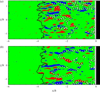
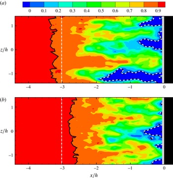
Contour plots of wall-normal vorticity (
 $\unicode[STIX]{x1D714}_{y}h/U_{\infty }$
) at the same two instants as in figure 13 are shown in figure 15 along with the shock location (
 $x_{s}^{sp}$
) and the line demarcating the recirculation region (
 $x_{r}^{sp}$
). Downstream of the shock line (
 $x_{s}^{sp}$
), both clockwise and anti-clockwise vorticity (
 $\unicode[STIX]{x1D714}_{y}h/U_{\infty }$
) are seen, with very little seen ahead of the shock for the chosen contour levels. This is the vorticity present in the upstream boundary layer and is lifted up as it crosses the shock (
 $x_{s}^{sp}$
) consistent with the broad picture of strong vortices seen downstream of the separation line in the simulation of Priebe & Martin (Reference Priebe and Martin2012).
Two instantaneous wall-normal vorticity (
 $\unicode[STIX]{x1D714}_{y}h/U_{\infty }$
) contour plots in the
 $x$
–
 $z$
plane at
 $y/h=0.25$
. Blue represents clockwise and red represents anti-clockwise vorticity. In the figure, the white dashed line represents the
 $u=0$
contour or the recirculation line (
 $x_{r}^{sp}$
) and the black continuous line represents the
 $u=0.8U_{\infty }$
condition that represents the shock location (
 $x_{s}^{sp}$
). The two cases shown correspond to the same instants as in figure 13. The contour levels shown correspond to
 $\unicode[STIX]{x1D714}_{y}h/U_{\infty }$
of
 $\pm$
2.

In the example, instantaneous streamwise velocity (
 $u/U_{\infty }$
) fields shown in figure 13, the spanwise-averaged shock location (
 $\overline{x_{s}^{sp}}$
) is approximately
 $-3.8h$
in both cases. To help understand the reason for the streamwise motions of the shock, we present in figure 16, two example instantaneous streamwise velocity (
 $u/U_{\infty }$
) fields corresponding to upstream (in a) and downstream (in b) positions of the shock. In both plots, apart from the instantaneous shock line shown in black (
 $x_{s}^{sp}$
), we also show the time-averaged location of the shock by a dot-dashed white line to help see the streamwise shock motions clearly. These fields show as in the previous cases that the instantaneous shock is relatively two-dimensional with small wrinkling of the shock. The reverse flow area in this plane (
 $A^{sp}$
) is higher in (a), but not very significantly compared to (b). It appears that the more important difference between the two is the fact that the most upstream point of the reverse flow denoted as
 $x_{r,min}^{sp}$
is considerably more upstream in (a), with
 $x_{r,min}^{sp}/h\approx -3.5$
, compared to
 $x_{r,min}^{sp}/h\approx -2.5$
in (b). We see this across many instantaneous fields, and this will be reflected further in the next section in conditionally averaged field based on this criterion and in the corresponding correlation coefficient. These spanwise instantaneous fields show that the shock is responding in a more global way to the recirculation region, and not locally at a given spanwise location. Hence, velocity fields in the wall-normal (
 $x$
–
 $y$
) plane can show some differences in shock location even when the recirculation region at that spanwise location is somewhat similar.
Two instantaneous streamwise velocity (
 $u/U_{\infty }$
) contours corresponding to upstream (in a) and downstream (in b) positions of the shock. Although both have a relatively similar sized recirculation region, the shock location is very different. The shock is pushed far upstream in (a) when the most upstream location of the recirculation region (
 $x_{r,min}^{sp}$
) is far upstream. In both plots, the continuous black line represents shock location (
 $x_{s}^{sp}$
), the dashed white line represents the recirculation line (
 $x_{r}^{sp}$
) and the dot-dashed line represents the time-averaged location of the shock.

Sample instantaneous streamwise velocity (
 $u/U_{\infty }$
) contours in the spanwise plane at (a)
 $y/h=0.5$
, (b)
 $y/h=0.75$
and (c)
 $y/h=1.0$
. In each of the plots, the continuous black line represents the shock location (
 $x_{s}^{sp}$
), the dashed white line represents the recirculation line (
 $x_{r}^{sp}$
), and the white dot-dashed line represents the time-averaged location of the shock.

(a) Variation of the spanwise-averaged value of the shock location (
 $\overline{x_{s}^{sp}}$
), the spanwise-averaged recirculation line (
 $\overline{x_{r}^{sp}}$
) and the average recirculation area (
 $A^{sp}$
) with the wall-normal coordinate
 $y/h$
. (b) Variation of the spanwise root-mean-square (spatial fluctuation) of the shock (
 $x_{s,rms}^{sp}$
) and the spanwise root-mean-square (spatial fluctuation) of the recirculation line with the wall-normal coordinate
 $y/h$
.

Apart from
 $y/h=0.25$
, measurements have also been done at other wall-normal planes. Sample instantaneous streamwise velocity contour plots at wall-normal locations of
 $y/h=0.5$
, 0.75 and 1 are shown in figure 17. As in the previous figure, the shock location (
 $x_{s}^{sp}$
) and the recirculation line (
 $x_{r}^{sp}$
) are shown in each case, along with the time-averaged location of the shock at that wall-normal location (dot-dashed white line). The shock location (
 $x_{s}^{sp}$
) in these cases, which are at the edge of the boundary layer or outside, is determined using a threshold that is 90 % of the free-stream velocity, while the recirculation location (
 $x_{r}^{sp}$
) is determined as before using the
 $u=0$
condition. It is clear from the plots that as the wall-normal location is increased, the extent of reverse flow is smaller, with these regions being closer to the step. The recirculation line continues to be highly three-dimensional at all
 $y/h$
locations. The shock location also moves closer to the step with increasing
 $y/h$
. In all cases, the spanwise ripples of the shock are in general much smaller than that of the recirculation line and appear to further reduce with
 $y/h$
.
We now proceed to present the variation of the shock location (
 $x_{s}^{sp}$
) and the recirculation line (
 $x_{r}^{sp}$
) with the wall-normal coordinate
 $y/h$
. Figure 18(a) shows the variation of the mean shock location (
 $\overline{x_{s}^{sp}}$
), the averaging here being done both spatially in the spanwise direction and temporally over all the fields obtained. The figure clearly shows that the mean shock location shifts downstream at higher wall-normal locations consistent with the velocity fields shown in figure 17, and the general oblique nature of the shock seen in the cross-stream fields. The spanwise variation of the shock (or ripples of the shock) is characterized by the spatial root-mean-square of the shock location, which has then been averaged over all the different instantaneous fields to obtain
 $x_{s,rms}^{sp}$
, as shown in figure 18(b). As may be seen from the plot, at
 $y/h=0.25$
,
 $x_{s,rms}^{sp}$
is approximately
 $0.25h$
, and reduces gradually with
 $y/h$
to approximately
 $0.2h$
at
 $y/h=1.0$
. This extent of the ripple in the shock is in reasonable agreement with values reported in Wu & Martin (Reference Wu and Martin2008).
The variation of the mean and spatial root-mean-square of the recirculation line (
 $x_{r}^{sp}$
) with
 $y/h$
is also shown in figure 18(a,b), respectively. The recirculation region decreases with height and this can be seen in the mean value of the recirculation line (
 $\overline{x_{r}^{sp}}$
) that goes from approximately
 $-2h$
towards zero as the height (
 $y/h$
) increases from 0.25 to 1. Another measure of the mean recirculation region location is the negative of the normalized mean recirculation region area in this plane (
 $-A^{sp}/h$
), as
 $A^{sp}$
is the recirculation region area in this spanwise plane calculated per unit spanwise length. The small differences between (
 $-A^{sp}/h$
) and
 $\overline{x_{r}^{sp}}/h$
is related to the method of calculating
 $x_{r}^{sp}$
, which is done by calculating the most upstream location of the recirculation line. The inherent assumption here is that all the downstream points at that spanwise (
 $z$
) location have
 $u<0$
, which is not necessarily the case as seen in the instantaneous velocity fields shown earlier. Hence,
 $-A^{sp}/h$
is a better measure of the mean recirculation location, and is slightly closer to the step (
 $x=0$
) than
 $\overline{x_{r}^{sp}}$
, as may be seen in figure 18(a). The spanwise variation in the recirculation line represented as
 $x_{r,rms}^{sp}$
is shown in figure 18(b). As seen earlier in the instantaneous plots shown in figure 13, this is much larger than for the shock at
 $y/h=0.25$
, with this value being approximately 0.7 as compared to a value of approximately 0.25 for the shock. As
 $y/h$
increases, the variations of the recirculation line in the spanwise direction decrease rapidly, approaching zero at
 $y/h=1.0$
.
In summary, the spanwise instantaneous fields indicate that the shock is relatively two-dimensional with small spanwise ripples, while the separation region is highly three-dimensional with very large spanwise variations that are approximately three times the shock variations in the spanwise direction.
5.2 Conditionally averaged fields
We present here conditionally averaged fields corresponding to both local and global influences; this terminology coming from Ganapathisubramani et al. (Reference Ganapathisubramani, Clemens and Dolling2009). We begin with local influences, namely the effect of low- and high-speed streaks in the boundary layer, and then move on to globally averaged (or spanwise-averaged) quantities.
We present in figure 19, conditionally averaged fields based on local line-averaged boundary layer velocity
 $u_{l}^{\prime }$
at the central span location (
 $z=0$
). In the figure, (a) corresponds to significantly negative
 $u_{l}^{\prime }$
(
 $u_{l}^{\prime }<-1.5\unicode[STIX]{x1D70E}$
), and (b) corresponds to significantly positive
 $u_{l}^{\prime }$
(
 $u_{l}^{\prime }>+1.5\unicode[STIX]{x1D70E}$
) (
 $\unicode[STIX]{x1D70E}$
 $=$
root-mean-square of
 $u_{l}^{\prime }$
in time). In both cases, we have stopped the colour contours at
 $u/U_{\infty }$
of 0.8, which acts as a surrogate for the shock at this
 $y/h$
, as already discussed earlier. One can clearly see from the plot that when
 $u_{l}^{\prime }$
is low (in a), corresponding to a low-speed streak, the shock is locally pulled upstream, while when
 $u_{l}^{\prime }$
is high (in b), corresponding to a high-speed streak, the shock is pushed downstream. This plot is very similar to the plot of Ganapathisubramani et al. (Reference Ganapathisubramani, Clemens and Dolling2007) for a compression ramp, and clearly shows as stated in their paper, that the shock within the boundary layer is considerably affected by the low- and high-speed streaks. The shock foot ripples thus appear to be strongly correlated to the presence of low- and high-speed streaks in the incoming boundary layer. It may be noted here that this observation is also likely related to the convex/concave shock corrugation seen in the canonical shock–turbulence interaction problem (Larsson & Lele Reference Larsson and Lele2009). We now present conditionally averaged fields based on the global or spanwise-averaged boundary layer fluctuation
 $\overline{u_{l}^{\prime }}$
in figure 20. In the figure, (a) corresponds to significantly negative
 $\overline{u_{l}^{\prime }}$
(
 $\overline{u_{l}^{\prime }}<-1.5\unicode[STIX]{x1D70E}$
) and (b) corresponds to significantly positive
 $\overline{u_{l}^{\prime }}$
(
 $\overline{u_{l}^{\prime }}>+1.5\unicode[STIX]{x1D70E}$
) (
 $\unicode[STIX]{x1D70E}$
 $=$
root-mean-square of
 $\overline{u_{l}^{\prime }}$
in time). Here, and in the other globally averaged quantities throughout this paper, we choose the range in the spanwise direction to be
 $-1<z/h<1$
, which represents the central 40 % of the total span of the FFS, where
 $\overline{u}$
is nearly independent of span (§ 2.3). This is to minimize any edge effects that may be present towards the ends of the FFS model. The spanwise-averaged shock location corresponding to the lower than mean value condition (in a) and higher than the mean value condition (in b) denoted as
 $\overline{x_{s,-}^{sp}}$
and
 $\overline{x_{s,+}^{sp}}$
, respectively, and given in table 5. The two conditional fields show some differences in the spanwise-averaged shock location with respect to each other (
 $\overline{x_{s,-}^{sp}}$
,
 $\overline{x_{s,+}^{sp}}$
), and the global mean shock location (
 $\overline{x_{s}^{sp}}$
) indicated by a white dot-dashed line in figure 20 at
 $x/h\approx -3.9$
. However, the change in spanwise-averaged shock locations between the two conditionally averaged fields (
 $\overline{x_{s,-}^{sp}}$
,
 $\overline{x_{s,+}^{sp}}$
) is small at approximately
 $0.2h$
. This indicates that the large-scale streamwise shock motions that are considerably larger and closer to
 $1h$
are not likely to be well correlated to the global or spanwise-averaged
 $\overline{u_{l}^{\prime }}$
.
Conditionally averaged streamwise velocity (
 $u/U_{\infty }$
) contours based on local line-averaged boundary layer velocity
 $u_{l}^{\prime }$
at the central span location (
 $z=0$
). Condition corresponding to low values of
 $u_{l}^{\prime }$
is shown in (a), and corresponding to higher
 $u_{l}^{\prime }$
is shown in (b). In both cases, the colour contours are stopped at
 $u/U_{\infty }$
of 0.8, which corresponds to the shock condition at this
 $y/h$
of 0.25. One can clearly see from the plot that when
 $u_{l}^{\prime }$
is low, the shock is locally pulled upstream, while when
 $u_{l}^{\prime }$
is high, the shock is locally pushed downstream.

Conditionally averaged streamwise velocity (
 $u/U_{\infty }$
) contours based on spanwise-averaged boundary layer velocity (
 $\overline{u_{l}^{\prime }}$
) between
 $-1<z/h<1$
at
 $y/h=0.25$
. Condition corresponding to low values of
 $\overline{u_{l}^{\prime }}$
is shown in (a), and corresponding to higher
 $\overline{u_{l}^{\prime }}$
is shown in (b). In both plots, the continuous black line represents shock location (
 $x_{s}^{sp}$
), the dashed white line represents the recirculation line (
 $x_{r}^{sp}$
) and the dot-dashed line represents the time-averaged location of the shock (
 $\overline{x_{s}^{sp}}$
).

Spanwise-averaged shock location (
 $\overline{x_{s}^{sp}}/h$
) for conditionally averaged fields based on global influence parameters that take into account data from different spanwise locations. The three global influence parameters considered here are the spanwise-averaged boundary layer fluctuations (
 $\overline{u_{l}^{\prime }}$
), the recirculation region area (
 $A^{sp}$
) and the most upstream point of the recirculation region (
 $x_{r,min}^{sp}$
). The correlation coefficients between the spanwise-averaged shock (
 $x_{s}^{sp}$
) and each of the three global influence parameters are also shown. In the table,
 $\overline{x_{s+}^{sp}}$
and
 $\overline{x_{s-}^{sp}}$
denote the spanwise-averaged shock location corresponding to conditionally averaged fields for high and low values of the corresponding global parameter. All the data in the table are calculated for
 $y/h=0.25$
and for
 $-1<z/h<+1$
.

Conditionally averaged streamwise velocity (
 $u/U_{\infty }$
) contours based on most upstream location of the recirculation line (
 $x_{r,min}^{sp}$
) between
 $-1<z/h<1$
at
 $y/h=0.25$
. Condition corresponding to low values of
 $x_{r,min}^{sp}$
is shown in (a), and corresponding to higher
 $x_{r,min}^{sp}$
is shown in (b). With this condition, we find a significant difference in the shock location between the two conditionally averaged fields, with a difference of about
 $0.61h$
. In both plots, the continuous black line represents shock location (
 $x_{s}^{sp}$
), the dashed white line represents the recirculation line (
 $x_{r}^{sp}$
) and the dot-dashed line represents the time-averaged location of the shock (
 $\overline{x_{s}^{sp}}$
).

As suggested by the cross-stream conditional fields, we would expect the shock (
 $x_{s}^{sp}$
) to be better correlated to the recirculation region (
 $x_{r}^{sp}$
) than the boundary layer velocity (
 $u_{l}^{\prime }$
). Since the shock (
 $x_{s}^{sp}$
) is relatively two-dimensional, we would expect that a global measure of the recirculation region would be better correlated to the shock location. A natural measure for this would be the recirculation area in this spanwise plane (
 $A^{sp}$
), which is also similar to the spanwise-averaged recirculation line (
 $\overline{x_{r}^{sp}}$
), as shown in figure 18(a). Although, using
 $A^{sp}$
as the condition does slightly increase the differences in the spanwise-averaged shock location between the small and large
 $A^{sp}$
conditional fields to 0.27, from 0.21 for conditions based on
 $\overline{u_{l}^{\prime }}$
, as shown in table 5, it is still not as large as one might expect. This indicates that the spanwise-averaged recirculation is also not well correlated to the large-scale streamwise motions of the shock.
A better global parameter that may be responsible for the large-scale shock motions is the condition based on the most upstream location of the recirculation line denoted as
 $x_{r,min}^{sp}$
. This can be seen from the example instantaneous streamwise velocity (
 $u/U_{\infty }$
) fields corresponding to upstream and downstream positions of the shock shown in figure 16. As discussed earlier, there is clearly a large difference between the two fields in the most upstream point of the reverse flow
 $x_{r,min}^{sp}$
. In (a),
 $x_{r,min}^{sp}$
is approximately
 $-3.5h$
, while in (b) it is approximately
 $-2.5h$
. We present conditionally averaged fields based on
 $x_{r,min}^{sp}$
between
 $-1<z/h<+1$
in figure 21. In the figure, (a) corresponds to fields that are more than 1.5 standard deviations below the mean value of
 $x_{r,min}^{sp}$
and (b) corresponds to fields that are more than 1.5 standard deviations greater than the mean value. For each of the two conditions, we have averaged approximately 35 fields that satisfy the respective conditions. We find now that with this condition, there is a significant difference in the spanwise-averaged shock location between the two conditionally averaged fields, with a difference of
 $0.61h$
(see table 5), which is considerably larger than for the previous conditions. The conditionally averaged field in (a) indicates that when some part of the recirculation region is very upstream, it appears to consistently correspond to the nearly two-dimensional shock being upstream, resulting in a far upstream position of the shock in the conditionally averaged field. On the other hand, in (b), when
 $x_{r,min}^{sp}$
is reasonably high, the recirculation region does not extend as much upstream, and the resulting conditional average shows that the shock is quite downstream. These conditionally averaged fields thus show that the most upstream point of the recirculation region (
 $x_{r,min}^{sp}$
) is likely to be well correlated to the large-scale shock motions.
Two instantaneous streamwise velocity (
 $u/U_{\infty }$
) contours corresponding to far upstream (in a) and far downstream (in b) locations of the shock at
 $y/h=0.75$
. The shock is pushed far upstream in (a) when the most upstream location of the recirculation region (
 $x_{r,min}^{sp}$
) is far upstream. In both plots, the continuous black line represents shock location (
 $x_{s}^{sp}$
), the dashed white line represents the recirculation line (
 $x_{r}^{sp}$
) and the white dot-dashed line represents the time-averaged location of the shock (
 $\overline{x_{s}^{sp}}$
).

5.3 Correlation coefficient
The calculation of correlations in the spanwise view (
 $x$
–
 $z$
) plane can be done in two ways, which we refer to as the local influence and the global influence, using the terminology of Ganapathisubramani et al. (Reference Ganapathisubramani, Clemens and Dolling2009). In the case of local influence, the correlation coefficient is determined using quantities at a given spanwise location, and is in principle the same as the correlations obtained from the cross-stream (
 $x$
–
 $y$
) plane PIV results in a single spanwise location. On the other hand, correlations calculated using the global influence, take in to account data from different spanwise locations. A common methodology of doing this, as discussed in Ganapathisubramani et al. (Reference Ganapathisubramani, Clemens and Dolling2009), would be the use of spanwise-averaged quantities. Given our interest in understanding what drives the approximately two-dimensional shock motions, the spanwise-averaged shock location
 $\overline{x_{s}^{sp}}$
is used as the primary quantity of interest. The correlations of
 $\overline{x_{s}^{sp}}$
with the spanwise-averaged boundary layer fluctuations
 $\overline{u_{l}^{\prime }}$
, the recirculation region area
 $A^{sp}$
and the most upstream point of the recirculation region
 $x_{r,min}^{sp}$
are presented in table 5 for
 $y/h=0.25$
. The correlation coefficient values of the spanwise-averaged boundary layer fluctuations (
 $\overline{u_{l}^{\prime }}$
) and recirculation region area (
 $A^{sp}$
) with the spanwise-averaged shock location (
 $\overline{x_{s}^{sp}}$
), are found to be 0.65 and
 $-$
0.18, respectively. Although this suggests a good correlation between the boundary layer fluctuations and the shock motions, it is not necessarily related to the large-scale shock motions that we are primarily interested in. This is clear from the conditionally averaged fields based on
 $\overline{u_{l}^{\prime }}$
that show only small differences of about
 $0.21h$
in the spanwise-averaged shock location (
 $\overline{x_{s}^{sp}}$
), as also shown in table 5. Hence, although its correlation value is high,
 $\overline{u_{l}^{\prime }}$
does not seem to be responsible for large-scale motions of the shock. In the case of the recirculation region area
 $A^{sp}$
, the correlation is quite low at approximately
 $-$
0.18, and the conditionally averaged fields for large and small values of
 $A^{sp}$
, show only small differences of approximately
 $0.27h$
in the spanwise-averaged shock location (
 $\overline{x_{s}^{sp}}$
). Hence, this also does not seem to be responsible for large-scale motions of the shock.
On the other hand, the most upstream point of the recirculation region (
 $x_{r,min}^{sp}$
) exhibits both a large correlation value of approximately 0.56, and the conditionally averaged fields show a large difference of approximately
 $0.61h$
in the spanwise-averaged shock location (
 $\overline{x_{s}^{sp}}$
). Hence, the most upstream point of the recirculation region (
 $x_{r,min}^{sp}$
) seems to be the parameter that is well correlated to the large-scale motions of the shock. The conditional fields shown so far are at
 $y/h=0.25$
(or
 $y/\unicode[STIX]{x1D6FF}=0.5$
), which is within the boundary layer. To emphasize the point that the most upstream point of the recirculation region (
 $x_{r,min}^{sp}$
) is indeed important, we show in figure 22, example instantaneous spanwise fields outside the boundary layer corresponding to far upstream and far downstream locations of the shock. This corresponds to a wall-normal location of
 $y/h=0.75$
(or
 $y/\unicode[STIX]{x1D6FF}=1.5$
). This is high enough to be outside the boundary layer, which is nominally up to
 $y/h=0.5$
(or
 $y/\unicode[STIX]{x1D6FF}=1.0$
), and still within the separation bubble. When the shock is far upstream (in a), one can clearly see that the most upstream point of the relatively thin recirculation region (
 $x_{r,min}^{sp}$
) is also far upstream. On the other hand, when the shock is downstream (in b), the most upstream location of the recirculation region (
 $x_{r,min}^{sp}$
) is far downstream, almost close to the step. These fields further emphasize that it is the global most upstream location of the recirculation region (
 $x_{r,min}^{sp}$
) that is likely to have the biggest correlation to the large-scale spanwise-averaged (
 $\overline{x_{s}^{sp}}$
) motions of the shock.
6 Discussion
The present PIV measurements in the cross-stream or wall-normal (
 $x$
–
 $y$
) plane and spanwise (
 $x$
–
 $z$
) plane show different features of the shock wave–boundary layer interactions ahead of a FFS. In the case of the wall-normal plane, the measurements show the distinct difference between the shock measured outside the boundary layer (
 $x_{s}$
), in contrast to the shock foot (
 $x_{sf}$
) determined from velocity data within the boundary layer. The shock location (
 $x_{s}$
) is found to be well correlated to the downstream recirculation region area (
 $A$
) and not to the boundary layer velocity fluctuations (
 $u_{l}^{\prime }$
), as also seen from the two conditionally averaged fields. On the other hand, the shock foot location (
 $x_{sf}$
) is found to be better correlated to the boundary layer velocity fluctuations (
 $u_{l}^{\prime }$
), than with the recirculation region area (
 $A$
), although the latter also has a significant effect.
The above results may be compared with those from the compression ramp and the impinging–reflecting shock cases, which have been studied in more detail. For the shock outside the boundary layer, both Piponniau et al. (Reference Piponniau, Dussauge, Debiève and Dupont2009) and Priebe & Martin (Reference Priebe and Martin2012) have shown that the separation bubble or recirculation region area is important in deciding the location of the shock ahead of the separation bubble. In contrast, the measurements of Ganapathisubramani et al. (Reference Ganapathisubramani, Clemens and Dolling2009) have highlighted the importance of upstream boundary layer velocity fluctuations on the surrogate separation (or shock foot) location determined from velocity data within the boundary layer. In the present case, this is consistent with the effect of the upstream boundary layer fluctuations on the shock foot.
The present spanwise PIV measurements show that there are large spanwise variations in the recirculation or the
 $u=0$
line, as shown for example in figure 16, while the shock is more two-dimensional, although it has spanwise ripples. The spanwise ripples of the shock within the boundary layer are seen to be well correlated to the upstream boundary layer streaks, as shown from conditional fields, consistent with the measurements of Ganapathisubramani et al. (Reference Ganapathisubramani, Clemens and Dolling2007). These spanwise instantaneous fields also indicate that the approximately two-dimensional shock is responding in a more global way to the recirculation region, and not locally at a given spanwise location. Hence, velocity fields in the wall-normal (
 $x$
–
 $y$
) plane, at a given spanwise location, can show differences in shock location even when the recirculation region is similar. This is likely to be one of the factors leading to lower correlations between the shock (or shock foot) and the recirculation region area (
 $A$
) in the
 $x$
–
 $y$
plane, which is approximately
 $-$
0.26. In particular, we find from spanwise (
 $x$
–
 $z$
) plane measurements, that it is the most upstream location of the relatively thin regions of recirculation (
 $x_{r,min}^{sp}$
) that is well correlated to the streamwise location of the shock. Using this global criterion, we find that the correlation increases from approximately
 $-$
0.26 to 0.56. It may be noted that all correlations presented in this study are calculated from data at the same time instant. As shown by Wu & Martin (Reference Wu and Martin2008) and Ganapathisubramani et al. (Reference Ganapathisubramani, Clemens and Dolling2009), the correlation coefficients will be higher if a time lag, of the order of approximately
 $7\unicode[STIX]{x1D6FF}/U_{\infty }$
, is used corresponding to the time taken for example of an upstream structure in the boundary layer to effect the shock position. The values obtained at the same instant, corresponding to zero time lag, are however quite indicative as shown by the same two studies.
The spanwise organization of the flow has been studied by Ganapathisubramani et al. (Reference Ganapathisubramani, Clemens and Dolling2007), Ganapathisubramani et al. (Reference Ganapathisubramani, Clemens and Dolling2009) and Priebe & Martin (Reference Priebe and Martin2012). Ganapathisubramani et al. (Reference Ganapathisubramani, Clemens and Dolling2009) have commented on the relatively stronger local effect of the upstream boundary layer, than the global or spanwise-averaged effect of the boundary layer. In the present case of the FFS, we again see a strong local effect of the upstream boundary layer on the shock foot location, and a weaker effect of the global or spanwise-averaged boundary layer on the shock, consistent with their results. Priebe & Martin (Reference Priebe and Martin2012) from their DNS studies have also discussed spanwise variations and coherence of the shock and wall pressure spectra. In their case, they state that ‘at low-frequency the shock in the free-stream and the recirculation bubble are roughly two dimensional, at least up to the corner’. Further downstream, closer to reattachment, three-dimensional effects are seen to be important. In our case, the instantaneous recirculation region appears to be highly three-dimensional, with long relatively thin regions of recirculation extending far upstream.
The thin long regions of recirculation seen suggest the strong possibility of the presence of large-scale three-dimensional structures in this region, and we shall now present results supporting this by showing the presence of coherent vortical structures in the
 $x$
–
 $z$
plane using the swirl strength criterion of Adrian, Meinhart & Tomkins (Reference Adrian, Meinhart and Tomkins2000). For this, the eigenvalues of the two-dimensional velocity gradient tensor (
 $\unicode[STIX]{x1D61A}_{ij}$
) were evaluated, with the swirl strength being the imaginary part of the eigenvalue. Figure 23 shows two examples of the zoomed in view of the instantaneous velocity field after subtracting the convection velocity of the point with the highest local swirl strength or the centre of the vortex (marked by ●) in the spanwise (
 $x$
–
 $z$
) plane at
 $y/h=0.5$
. The black line in the plots represents the
 $u=0$
contour or the recirculation line showing the relatively thin narrow region of
 $u<0$
in each case. In the frame of reference of the vortex, these examples show the presence of not one, but two counter-rotating structures close to the most upstream location of the thin recirculation regions, with one vortex on either side of this region. As expected, these counter-rotating vortex pairs induce low-momentum fluid in its centre, which causes a large negative peak in the fluctuating streamwise velocity. We identify this minimum streamwise velocity location as the centre point between the counter-rotating vortices, as marked by the solid square (▪) in each of the example fields in figure 23. We find that these counter-rotating structures are of different sizes, their centre to centre distance varying from approximately 0.5 to 1 step height. These fields indicate that there is a strong counter-rotating vortex, in the spanwise (
 $x$
–
 $z$
) plane, around the most upstream location of the thin recirculation regions that extend far upstream. This is suggestive of the fact that the thin long recirculation regions ahead of the step are related to the presence of three-dimensional structures.
The reason for the presence of these large-scale three-dimensional structures in the recirculation region is not clear at present. One possibility is the development of Görtler instability as the boundary layer is turned by the time-averaged dividing streamline, with this streamline having a concave nature from approximately
 $x/h\approx -4$
to
 $x/h\approx -2.5$
, where we can expect the Görtler instability to develop (Saric Reference Saric1994). The smallest radius of curvature of the mean dividing streamline is found to occur at
 $x/h\approx -3$
, with the corresponding Görtler number (
 $G=(U_{\infty }\unicode[STIX]{x1D703}/\unicode[STIX]{x1D708})(\unicode[STIX]{x1D703}/R)^{(0.5)}$
) being approximately 300 indicating that this is certainly a possibility (
 $\unicode[STIX]{x1D703}$
 $=$
boundary layer momentum thickness,
 $R$
 $=$
radius of curvature of the mean dividing streamline). However, it should be noted that this is based on the mean dividing streamline, which is only present in a time-averaged sense. In reality, the flow turning in the present case varies considerably with time, as the flow in the recirculation region is highly unsteady. In addition, as shown in Spall & Malik (Reference Spall and Malik1989), the effects of compressibility on the instability can be significant, leading to Mach number and wall temperature effects. Apart from the Görtler instability, another possibility is that the shedding of vorticity from the recirculation region (as in Pearson et al. (Reference Pearson, Goulart and Ganapathisubramani2013) for subsonic FFS) can also become three-dimensional, as seen for example in the case of the backward-facing step case (Lee, Ahn & Sung Reference Lee, Ahn and Sung2004; Sheu & Rani Reference Sheu and Rani2006).
A simplified schematic of the flow field ahead of the step is presented in figure 24 showing the observed counter-rotating pair in the
 $x$
–
 $z$
plane and its correlation to the recirculation region and the shock and shock foot locations.
Two examples of the instantaneous velocity field zoomed in around the thin recirculation regions in the spanwise (
 $x$
–
 $z$
) plane at
 $y/h=0.5$
. In both cases, the velocity field is shown after subtracting the convection velocity of the point with the highest local swirl strength or the centre of the vortex (marked by ●). The black line in the plots represents the recirculation line (
 $u=0$
). In this frame of reference, two counter-rotating vortices can be seen close to the most upstream location of the thin recirculation region with the solid square (▪) denoting the minimum streamwise velocity location or the centre between the counter-rotating vortices.

Schematic of shock wave–boundary layer interactions over a FFS showing the main features of the flow. In (a), the most upstream location of the recirculation region (black dashed line) is relatively upstream, pushing the shock upstream, while in (b), the recirculation region is relatively downstream with the shock position also being downstream. The time-averaged shock location is shown by the red line. In both cases, the recirculation region ahead of the step is highly three-dimensional, while the shock has spanwise ripples that are well correlated to the streaks in the incoming boundary layer.

7 Conclusions
We study in the present work a Mach 2.5 flow over a FFS. The focus of the work is the flow ahead of the step, in particular, the unsteady interactions between the shock, the boundary layer and the separation bubble. The primary geometrical parameter in the problem is the ratio of the step height to the incoming boundary layer thickness,
 $h/\unicode[STIX]{x1D6FF}$
, which is fixed at 2 in the present study. This was chosen as it keeps both
 $h$
and
 $\unicode[STIX]{x1D6FF}$
comparable, while at the same time, the step protrudes out of the boundary layer, as in the compression ramp cases, mimicking in some way the well-studied case of the compression ramp. Results are presented from detailed PIV measurements in two orthogonal planes, one perpendicular to the lower wall (
 $x$
–
 $y$
plane) and the other parallel to the lower wall (
 $x$
–
 $z$
plane), to gain a reasonable picture of the whole flow field. Unsteady wall pressure measurements have also been done to get the dominant frequencies of the shock motions.
The mean velocity field in the central cross-stream or wall-normal (
 $x$
–
 $y$
) plane shows that the incoming boundary layer separates upstream of the step forming a large separation bubble ahead of the step. Due to its large size in the wall-normal direction (
 $y$
), this separation bubble can be relatively well resolved in measurements compared to the compression ramp cases. Surface oil flow visualization shows that the separation occurs at
 $4.1h$
upstream of the step. Wall pressure fluctuation spectra close to the separation location show a dominant frequency that is two orders of magnitude smaller than the characteristic frequency present in the incoming boundary layer (
 $U_{\infty }/\unicode[STIX]{x1D6FF}$
). This peak thus clearly corresponds to the low-frequency motions of the shock that has received a lot of recent attention (Clemens & Narayanaswamy Reference Clemens and Narayanaswamy2014).
Different schools of thought attribute the observed low-frequency shock motions to upstream influences in the incoming boundary layer or downstream influences originating in the separation bubble. Motivated by these debates, we extract from instantaneous PIV fields in the wall-normal (
 $x$
–
 $y$
) plane, parameters such as shock location (
 $x_{s}$
), an upstream line-averaged boundary layer velocity (
 $u_{l}^{\prime }$
) and a downstream separation bubble or recirculation region area (
 $A$
) defined as the region of negative streamwise velocities (
 $u<0$
). In addition to the shock location (
 $x_{s}$
) based on data from outside the boundary layer, we also define and extract a shock foot location (
 $x_{sf}$
) from data within the boundary layer.
Conditionally averaged velocity fields based on the incoming boundary layer velocity fluctuation (
 $u_{l}^{\prime }$
) and recirculation region area (
 $A$
) indicate that the shock location determined from data outside the boundary layer (
 $x_{s}$
) is correlated to the recirculation region area (
 $A$
) and not to the incoming boundary layer velocity fluctuation (
 $u_{l}^{\prime }$
). This is also supported by correlation coefficients between the shock location (
 $x_{s}$
) and the upstream boundary layer velocity fluctuation (
 $u_{l}^{\prime }$
) and downstream recirculation region (
 $A$
) parameters. The correlation between shock location (
 $x_{s}$
) and the recirculation area (
 $A$
) is found to be
 $-$
0.26, which is quite significant. On the other hand, the correlation between shock location (
 $x_{s}$
) and boundary layer velocity fluctuation (
 $u_{l}^{\prime }$
) is found to be only approximately
 $-$
0.03 suggesting that in the FFS case, it is the downstream influence which is important. This result appears at first to differ from the results of some recent studies on compression ramps such as those of Unalmis & Dolling (Reference Unalmis and Dolling1998), Andreopoulos et al. (Reference Andreopoulos, Agui and Briassulis2000), Beresh et al. (Reference Beresh, Clemens and Dolling2002) and Ganapathisubramani et al. (Reference Ganapathisubramani, Clemens and Dolling2007). However, this is not necessarily the case. In these earlier studies, the shock foot close to the lower wall was measured either from PIV or wall pressure fluctuations, and not necessarily the shock which is present a little further away from the wall and boundary layer. This can be seen from the present shook foot location (
 $x_{sf}$
) measured within the boundary layer, which shows significant differences due to the presence of low- and high-speed streaks in the boundary layer. The correlation coefficient between shock foot (
 $x_{sf}$
) and the boundary layer velocity fluctuations (
 $u_{l}^{\prime }$
) shows a high correlation coefficient of 0.55, while the correlation coefficient between shock foot (
 $x_{sf}$
) and the downstream bubble (
 $A$
) shows a correlation coefficient of -0.27. This indicates that the shock foot is well correlated to the boundary layer structures, while also being reasonably correlated to the recirculation bubble area. This suggests that the shock foot is more responsive to the boundary layer fluctuations consistent with the observations of Ganapathisubramani et al. (Reference Ganapathisubramani, Clemens and Dolling2007) in the case of the compression ramp, although the main separation shock measured well outside the boundary layer remains nearly unaffected by these fluctuations as shown by Priebe & Martin (Reference Priebe and Martin2012). We do not however imply that the shock (
 $x_{s}$
) has no connection with the upstream boundary layer. As suggested by Dussauge & Piponniau (Reference Dussauge and Piponniau2008), changes in the boundary layer can affect the separation bubble. Our results only indicate that the correlation between the shock measured well outside the boundary layer and the naturally occurring structures within the boundary layer is very weak.
Measurements have also been done in the spanwise (
 $x$
–
 $z$
) plane at different wall-normal (
 $y$
) locations. From these spanwise velocity fields, we determine the shock location (
 $x_{s}^{sp}$
) using a velocity threshold criterion, and also a recirculation line (
 $x_{r}^{sp}$
) defined as the zero streamwise velocity (
 $u=0$
) line. The recirculation line (
 $x_{r}^{sp}$
) is representative of the recirculation region area (
 $A$
) that was used in the wall-normal PIV measurements. Instantaneous velocity fields in the spanwise (
 $x$
–
 $z$
) plane show that the shock is nearly two-dimensional with small spanwise ripples of approximately
 $0.5h$
. On the other hand, the recirculation line marking the edge of the recirculation region (
 $u=0$
) is found to be highly three-dimensional with very large spanwise variations of the order of
 $3h$
. These spanwise instantaneous fields show that the approximately two-dimensional shock is responding in a more global way to the recirculation region, and not locally at a given spanwise location.
As suggested by the wall-normal conditional fields, we would expect the shock location (
 $x_{s}^{sp}$
) to be better correlated to the recirculation region (
 $x_{r}^{sp}$
) than the boundary layer velocity fluctuation (
 $u_{l}^{\prime }$
). Since the shock (
 $x_{s}^{sp}$
) is relatively two-dimensional, we would expect that a global measure of the recirculation region would be better correlated to the shock location. A natural measure for this would be the spanwise-averaged recirculation region (
 $\overline{x_{r}^{sp}}$
). However, we find that there is another measure that shows significantly higher correlations, and hence a larger difference between (
 $+/-$
) conditional fields. This is the condition based on the most upstream location of the recirculation line between
 $-1<z/h<1$
, which we denote as
 $x_{r,min}^{sp}$
. Using this global criterion, we find that the correlation between the shock and the recirculation region is approximately 0.56 compared to the value of approximately 0.26 from the local condition obtained from the cross-stream or wall-normal (
 $x$
–
 $y$
) plane measurements. Conditionally averaged fields based on
 $x_{r,min}^{sp}$
show a significant difference in the streamwise shock location of approximately
 $0.61h$
between high and low values of this condition. Instantaneous spanwise fields show that when some part of the recirculation region is far upstream (
 $x_{r,min}^{sp}$
is low), the nearly two-dimensional shock is also very upstream. On the other hand, when
 $x_{r,min}^{sp}$
is reasonably high, the recirculation region does not extend as much upstream, and the resulting shock is quite downstream. These results indicate that the most upstream point of the recirculation region (
 $x_{r,min}^{sp}$
) is well correlated to the shock location.
In summary, we present figure 24 that gives a schematic overview of the main results and our interpretation of the measurements. The two schematics shown correspond to a relatively upstream position of the shock (in a) and a relatively downstream position of the shock (in b). The main difference between the two is the most upstream location of the recirculation region (black dashed line) (
 $x_{r,min}^{sp}$
). When
 $x_{r,min}^{sp}$
is relatively upstream, the shock is also found to be more upstream, while when
 $x_{r,min}^{sp}$
is relatively downstream, the shock also moves downstream. In both cases, the recirculation region ahead of the step is highly three-dimensional, while the shock foot has smaller spanwise ripples that are well correlated to the streaks in the incoming boundary layer. Hence, the present results suggest that for the FFS configuration, it is the downstream effect caused by the separation bubble that is well correlated to the observed low-frequency shock motions. This appears consistent with the statements of Priebe & Martin (Reference Priebe and Martin2012) and Clemens & Narayanaswamy (Reference Clemens and Narayanaswamy2014) that in strongly separated cases, it is the downstream influence related to the instability of the separated region that is likely to be more important.