





1 Introduction
1.1 General overview
Shock-wave/turbulent-boundary-layer interactions (STBLI) occur in many high-speed applications such as air intakes, control surfaces and over-expanded nozzles. If the interaction is strong enough, the flow separates, resulting in a highly unsteady flow. Of particular interest are low-frequency components, i.e. phenomena with pertinent time scales much larger than those associated with the incoming turbulence. The associated dynamics, including unsteady thermo-mechanical loading and density fluctuations, can excite adverse structural responses, lead to loss of control authority, result in inefficient or even catastrophic inlet dynamics and exacerbate aero-optical distortion. Reviews by Dolling (Reference Dolling2001) and more recently Gaitonde (Reference Gaitonde2015) discuss progress in STBLI research and the challenges that lie ahead. Both emphasize low-frequency unsteady aspects as areas of major concern, requiring control techniques for their moderation. However, characterizing the dynamics of these phenomena, especially distinguishing causation from correlation, remains a challenging task – this has inhibited the development of an optimal strategy for flow control.
Recent representative experimental (Dupont, Haddad & Debiève Reference Dupont, Haddad and Debiève2006; Dupont et al. Reference Dupont, Piponniau, Sidorenko and Debiève2008; Ganapathisubramani, Clemens & Dolling Reference Ganapathisubramani, Clemens and Dolling2009; Piponniau et al. Reference Piponniau, Dussauge, Debieve and Dupont2009; Souverein et al. Reference Souverein, Dupont, Debiève, Van Oudheusden and Scarano2010) and computational (Pirozzoli & Grasso Reference Pirozzoli and Grasso2006; Touber & Sandham Reference Touber and Sandham2009; Agostini et al. Reference Agostini, Larchevêque, Dupont, Debiève and Dussauge2012; Grilli et al. Reference Grilli, Schmid, Hickel and Adams2012; Priebe & Martín Reference Priebe and Martín2012; Aubard, Gloerfelt & Robinet Reference Aubard, Gloerfelt and Robinet2013; Morgan et al. Reference Morgan, Duraisamy, Nguyen, Kawai and Lele2013; Priebe et al. Reference Priebe, Tu, Rowley and Martín2016) efforts have explored various aspects of STBLIs and several physical mechanisms have been proposed to explain the observed unsteadiness. These may be broadly classified into two main categories. The first underscores the upstream influence of the incoming turbulent boundary layer. For instance, Ganapathisubramani et al. (Reference Ganapathisubramani, Clemens and Dolling2009) demonstrated a correlation between the low-frequency response of the surrogate separation point and large-scale, low- and high-speed regions in the incoming turbulent boundary layer. The second considers downstream influence via coupling between the boundary layer, recirculation region and shock. In particular, Piponniau et al. (Reference Piponniau, Dussauge, Debieve and Dupont2009) built upon the analysis of Dupont et al. (Reference Dupont, Haddad and Debiève2006) to propose a model which explains breathing of the separation bubble and low-frequency shock motion in terms of fluid entrainment in the mixing layer, whereby fluid from the separation bubble is continuously entrained in the mixing layer, shed downstream and must be replenished at a time scale corresponding to the low-frequency shock oscillations. This second class of mechanisms has been demonstrated to exist even when the boundary layer is statistically free from noise near the low frequency of interest (Touber & Sandham Reference Touber and Sandham2009). It is generally accepted that while both classes of mechanisms contribute to the low-frequency shock dynamics, the second class becomes more dominant as the size of the time-mean recirculation region increases (Souverein et al. Reference Souverein, Dupont, Debiève, Van Oudheusden and Scarano2010; Clemens & Narayanaswamy Reference Clemens and Narayanaswamy2014). Morgan et al. (Reference Morgan, Duraisamy, Nguyen, Kawai and Lele2013) have recently evaluated the validity of many of these mechanisms through examination of an extensive large-eddy simulation (LES) database. Although these and subsequent studies find a correlation between the size of the ‘turbulent separation bubble’ and the longitudinal shock location, the driving mechanisms and a causal description of the low-frequency dynamics of the separation bubble remain unclear.
Additional theoretical and numerical tools, including stability analyses, have also been deployed to understand the physical origin of low-frequency shock unsteadiness. Concerning laminar interactions, Robinet (Reference Robinet2007) found a three-dimensional global instability through BiGlobal linear-stability analysis that led to self-sustained low-frequency oscillations when the incident shock exceeded a critical angle. Recently, Guiho, Alizard & Robinet (Reference Guiho, Alizard and Robinet2016) demonstrated that laminar SBLIs are globally stable to two-dimensional perturbations over a wide parameter space, behaving as globally stable selective amplifiers as opposed to unstable oscillators. Sansica, Sandham & Hu (Reference Sansica, Sandham and Hu2014) investigated the low-frequency response of a laminar SBLI to white-noise forcing through the solution to a non-modal initial value problem (IVP), rather than a modal eigenvalue problem (EVP) (as distinguished by Theofilis (Reference Theofilis2011)), exciting a mid-frequency Kelvin–Helmholtz (K–H) response as well as a low-frequency broadband response. This work was a natural extension of an earlier effort by Touber & Sandham (Reference Touber and Sandham2009), who perturbed the time-mean flow obtained from an LES of a turbulent SBLI using white noise to find an unstable, two-dimensional, global mode with a growth time scale similar to that observed in low-frequency bubble breathing. IVP perturbation analyses of the time-mean turbulent flow were also conducted by Pirozzoli et al. (Reference Pirozzoli, Larsson, Nichols, Bernardini, Morgan and Lele2010), who observed a similar unstable global mode. They corroborated their findings with a BiGlobal linear-stability analysis of the time-mean turbulent flow, which, in addition to an unstable non-oscillatory (zero-frequency) global mode, identified several weakly damped oscillatory modes resembling bubble breathing extracted from low-pass filtered LES flow fields. This analysis was extended by Nichols et al. (Reference Nichols, Larsson, Bernardini and Pirozzoli2017) who describe the STBLI as a weakly damped oscillator, sustained by forcing, with a non-oscillatory unstable global mode. Notably, Sartor et al. (Reference Sartor, Mettot, Bur and Sipp2015) did not observe this non-oscillatory unstable global mode in the analysis of a transonic STBLI, and they found the least stable eigenvalues unrelatable to observed experimental unsteadiness. These observations are reconcilable with the previous studies, since the Reynolds averaged Navier–Stokes (RANS) equations, not the Navier–Stokes equations, were linearized about the turbulent mean, itself obtained from a RANS calculation that converged to a steady solution. As Nichols et al. (Reference Nichols, Larsson, Bernardini and Pirozzoli2017) identified: the linearization of the RANS equations for such a solution should be globally stable. However, the same cannot be said for linearizing the RANS equations about a steady base flow that does not satisfy the steady RANS equations, which may give rise to unstable global modes (Sartor, Mettot & Sipp Reference Sartor, Mettot and Sipp2014). A unified theoretical basis for linearizing propagation equations about a steady base flow that is not a steady solution to the given propagation equations remains to be developed.
1.2 Current contribution
The present study seeks to build on this understanding of the steady, laminar or turbulent-mean, base flow (also referred to as the basic state) by applying, for the first time, a perturbation analysis to the evolving, unsteady STBLI. The goal is to examine the dynamic linear response (DLR) of the flow to identify mechanisms that result in the observed low-frequency dynamics. Specifically, we employ concepts developed for the analysis of nonlinear dynamical systems (Khalil Reference Khalil1996), including those of Lyapunov stability and Lyapunov exponents (Skokos Reference Skokos, Souchay and Dvorak2010; Pikovsky & Politi Reference Pikovsky and Politi2016). The analysis is accomplished through calculation of the evolution of forced and constrained linear perturbations of the time-resolved STBLI base flow. This technique for analysing flow stability may be classified as global (Theofilis Reference Theofilis2011), as opposed to local (Huerre & Monkewitz Reference Huerre and Monkewitz1990), and non-modal (Schmid Reference Schmid2007), as opposed to modal (Schmid & Henningson Reference Schmid and Henningson2001), following terminology described in the aforementioned references; it considers the global influence of the flow, and no ansatz of frequency-isolated modes is assumed, since intermodal frequency mixing will generally occur for linear perturbations of an unsteady base flow; such an occurrence may arise without any nonlinear interactions.
1.3 Dynamic linear response
In this framework, the base flow is the evolving, unsteady STBLI, as obtained from an LES of the Navier–Stokes equations in suitable fashion; the approach employed in this work is discussed in § 2. The dynamic linear response is then the statistical-ensemble description, including time-local, time-mean and spectral components, of the linear-perturbations evolving around the unsteady base flow subject to forcing; considerations concerning the extraction of coherent features of the turbulent flow and ensemble averaging are addressed by Hussain (Reference Hussain1986) and Jeong et al. (Reference Jeong, Hussain, Schoppa and Kim1997), respectively. Details of all aspects of the technique employed are presented in § 3. The dynamic linear response (§ 3.1) provides insight into the tendency of the evolving flow at different points in the low-frequency cycle, in turn aiding in the determination of causal mechanisms in the STBLI. Furthermore, through proper processing and interpretation of perturbation evolution, correlations between features of unsteadiness in the low-, mid- and high-frequency ranges can be discerned, as can the manner in which these linear tendencies contribute to the restoration (or otherwise) of the flow to its time-mean state.
Requirements for admissibility of perturbations for the dynamic linear response are similar to those for traditional stability analyses; they must satisfy the linearized Navier–Stokes (LNS) equations subject to forcing with specified boundary and initial conditions. With regard to the form of forcing, stability literature considers time harmonic, impulsive and stochastic variants (Schmid Reference Schmid2007). Our strategies are discussed in § 3.2 and include both band-limited white noise as well as ‘native’ forcing, which has the same spectral form as the local turbulent fluctuations. A key distinction of the present effort from traditional analyses is that since the base flow of interest is highly unsteady, the linearization must be performed about the time-evolving turbulent flow. The numerical technique used solves the LNS equations through a modification of the synchronized LES procedure (SLES) described by Unnikrishnan & Gaitonde (Reference Unnikrishnan and Gaitonde2015, Reference Unnikrishnan and Gaitonde2016), who developed it to track the evolution of wave packets originating from turbulent fluctuations in the core of a jet, to understand intermittent events in the acoustic near field. Like other IVP perturbation methods, results from SLES must be processed as a statistical ensemble and do not directly reveal modal information. However, given the prohibitive computational expense of methods which analyse three-dimensional steady base flows, e.g. TriGlobal (EVP) analyses (Theofilis Reference Theofilis2011), IVP methods are perhaps the only suitable techniques by which to probe time-dependent three-dimensional base flows.
Stability studies of time-dependent flows are relatively rare, and are generally focused on the non-modal stability of laminar flows. Time-dependent non-modal approaches may be generally classified as either examining the fundamental solution operator (Schmid Reference Schmid2007) or the adjoint equations, which are reviewed by Luchini & Bottaro (Reference Luchini and Bottaro2014). The success of these approaches in understanding time-dependent laminar base flows is discussed by Schmid (Reference Schmid2007). Briefly, the dynamic linear response facilitates exploration of the nature of the fundamental solution operator using an ensemble of IVPs, each corresponding to a specific realization of the base flow and forcing. Generally, the fundamental solution operator can describe the non-modal evolution of perturbations of steady or unsteady base flows, and it is often referred to as the Green’s function (Luchini & Bottaro Reference Luchini and Bottaro2014) or the propagator (Farrell & Ioannou Reference Farrell and Ioannou1996); it is analogous to a time-dependent resolvent operator (McKeon & Sharma Reference McKeon and Sharma2010) but is not restricted to harmonic behaviour in time. Specifically, for the complex flow considered, the fundamental solution operator is not explicitly calculated, as this would be prohibitive in an unsteady calculation with
 $\mathit{O}(10^{8})$
discrete degrees of freedom. Rather, the linear response is determined from a statistical-ensemble analysis of the propagated linear perturbations. That is, the linear response is identified through analysis of many realizations of linear perturbations (the evolution of which is specific to each forcing and base-flow realization) by invoking flow ergodicity over long duration.
The application of synchronized LES analysis to the wall-bounded, turbulent, separated flow encountered in STBLIs is not trivial since there are relatively large reversed flow regions and thin, high-gradient, subsonic layers near the wall, the chaotic nature of which leads to large perturbation growth rates. Perturbations growing to nonlinear magnitudes indicate that the synchronized simulations (the perturbed and base-flow realizations of the STBLI) decorrelate in time, as discussed in § 3.3. While these realizations remain statistically similar, the instantaneous difference between the two is no longer representative of the dynamic linear response of the STBLI. Since the time scales of perturbation growth to nonlinear magnitudes are later shown to be much shorter than the time scales of low-frequency mechanisms, a difficulty arises in acquiring the dynamic linear response of low-frequency mechanisms associated with the separation bubble and concomitant shock motion. To resolve this issue, § 3.3 introduces a procedure to linearly constrain perturbation growth and maintain linearity with respect to the base flow, enabling sustained long-time acquisition of the desired linear-perturbation data. This corresponds to the implicit addition of a forcing term to the governing equations that highlights the time-local tendency toward rapid linear growth, i.e. the influence of faster growing perturbations persists in time, while the influence of slower growing perturbations attenuates. The overall procedure of using two LES to extract the dynamic linear response is presented in § 3.4. When the linear constraint is applied, the SLES is then designated LC-SLES. In the context of Lyapunov stability, the effect of this linear constraint amounts to Lyapunov renormalization, which facilitates the identification of unstable linear dynamics associated with the largest Lyapunov exponent of the flow, as discussed in § 3.5 (Skokos Reference Skokos, Souchay and Dvorak2010; Pikovsky & Politi Reference Pikovsky and Politi2016).
1.4 Application to STBLI
The linearly constrained analysis is applied to the impinging STBLI, with emphasis on understanding upstream influence, separation bubble dynamics, vortex shedding and low-frequency shock motion. The specific problem considered is described in § 4, which includes an assessment of the base flow. Briefly, we consider an oblique shock wave generated by a
 $9^{\circ }$
wedge impinging on a Mach 2.33 (momentum thickness Reynolds number:
 $Re_{\unicode[STIX]{x1D703}}=2300$
) turbulent boundary layer, previously studied computationally by Mullenix & Gaitonde (Reference Mullenix and Gaitonde2013) and validated by comparison with experimental data obtained at The Ohio State University Gas Dynamics and Turbulence Laboratory (Webb, Clifford & Samimy Reference Webb, Clifford and Samimy2013). The effect of stronger interaction strength is also addressed with an
 $11^{\circ }$
wedge shock.
The results in § 5 first consider preliminary aspects of constrained and unconstrained perturbation evolution and subsequently address the physics of the low-frequency oscillations. For this, several cases are delineated in § 5.1, differing from each other primarily in the nature, location and duration of forcing. In § 5.2, the transient amplification without constraint is discussed to illustrate sensitivity of the chaotic flow to initial conditions, the extent of the linear growth domain, and to motivate and justify the constraining parameters chosen for subsequent work. Section 5.3 describes the statistically stationary state of the linearly constrained perturbations. The path by which the stationary state is achieved is first discussed in § 5.3.1, followed by a demonstration that the constraining technique recovers linearity in § 5.3.2. The response to different forcing parameters reveals the presence of self-sustaining linearly constrained perturbations in § 5.3.3. These observations are connected to the concepts of absolute and convective global instabilities discussed by Huerre & Monkewitz (Reference Huerre and Monkewitz1990) and Chomaz (Reference Chomaz2005), which we observe in the STBLI and undisturbed turbulent boundary layer, respectively; in response to forcing, absolutely unstable flows exhibit self-sustained oscillations, whereas convectively unstable flows respond as selective amplifiers. Additionally, these findings are related to the mean-flow stability results of Touber & Sandham (Reference Touber and Sandham2009), Pirozzoli et al. (Reference Pirozzoli, Larsson, Nichols, Bernardini, Morgan and Lele2010) and Nichols et al. (Reference Nichols, Larsson, Bernardini and Pirozzoli2017), in the context of shock motion asymmetry observed by Piponniau et al. (Reference Piponniau, Dussauge, Debieve and Dupont2009). Again employing the terminology of stability theory, the ‘receptivity’ of the turbulent flow is characterized in § 5.3.4 by examining the effect of forcing location on the perturbation field, using wall-normal velocity as a sample variable; the insensitivity to forcing facilitates confirmation of the absolute nature of the instability. We examine and correlate the spectral content of both the base-flow and perturbation fields in § 5.3.5, including the attenuation factor, which linearly enforces the perturbation constraint.
The final investigation in § 5.3.6 simultaneously decomposes the turbulent base-flow and perturbation fields through band-pass temporal filtering to generate insight into mechanisms that sustain coherent motion and low-frequency unsteadiness. Several bands are considered, each motivated by prominent frequency ranges identified in the literature, which collapse reasonably well when described by a Strouhal number based on the nominal length of the separation bubble,
 $L$
:
 $St_{L}=fL/U_{\infty }$
(Dussauge, Dupont & Debiève Reference Dussauge, Dupont and Debiève2006). Commonly, the low-frequency dynamics
 $(St_{L}\sim 0.03)$
are of most interest as this band corresponds to the relatively largest-scale coherent motion of the reflected shock. High–mid-frequency Kelvin–Helmholtz shedding along the separated shear layer
 $(St_{L}\sim 0.5)$
has also been observed and discussed (Agostini et al.
Reference Agostini, Larchevêque, Dupont, Debiève and Dussauge2012; Aubard et al.
Reference Aubard, Gloerfelt and Robinet2013). Additionally, we identify important dynamics at a low–mid frequency
 $(St_{L}\sim 0.1)$
, corresponding to oscillations of the separation bubble. In fact,
 $St_{L}\sim 0.1$
content is found in the recirculation region power spectra of many studies (Dupont et al.
Reference Dupont, Haddad and Debiève2006; Touber & Sandham Reference Touber and Sandham2009; Aubard et al.
Reference Aubard, Gloerfelt and Robinet2013), but it is often not discussed in detail. The high-frequency
 $(St_{L}\gtrsim 1)$
response of the shock to fine-scale boundary layer turbulence results in the least coherent (jittering) motion and is not considered a primary concern for analysis or control efforts.
We also discuss in § 5.3.6 the band-isolated dynamics of the base flow and perturbations in the context of a mass-depletion mechanism, e.g. the conceptual model of Piponniau et al. (Reference Piponniau, Dussauge, Debieve and Dupont2009). Such a model is consistent with the low-frequency dynamics; however, like Morgan et al. (Reference Morgan, Duraisamy, Nguyen, Kawai and Lele2013) we find that the ‘turbulent separation bubble’ responds more significantly at higher frequencies
 $(St_{L}\sim 0.1)$
than predicted by the model
 $(St_{L}\sim 0.03)$
. We discuss these observations in conjunction with the results of Kiya & Sasaki (Reference Kiya and Sasaki1985), who observe higher-frequency
 $(St_{L}\sim 0.1)$
content in low-speed separation bubbles.
Given the difficulty of trying to verify the causality of any single proposed mechanism driving the low-frequency shock unsteadiness, several authors have applied simpler stochastic models, describing the motion in terms of a first-order stochastic ordinary differential equation (ODE). Plotkin (Reference Plotkin1975) first postulated that the low-frequency motion could be described, assuming that the shock displaced from its time-mean position would be subject to a linear restoring mechanism. This model was later verified experimentally by Poggie & Smits (Reference Poggie and Smits2001) and more recently derived analytically with supporting assumptions validated through LES by Touber & Sandham (Reference Touber and Sandham2011). Sansica, Sandham & Hu (Reference Sansica, Sandham and Hu2016) also reproduced many of the key features of the oscillation by suitably forcing a laminar SBLI, showing that broadband low-frequency upstream content is not necessary to elicit a low-frequency response at the separation point. Rather the response can result from ‘forcing’ via transition downstream, which is then low-pass filtered by the interaction. To assess the accuracy of the assumptions employed in development of simplified models for low-frequency unsteadiness, § 5.3.6 also examines the perturbation dynamics at different phases of the low-frequency shock motion cycle to identify linear tendencies for restoration toward or departure from the mean state. We discuss the accuracy of the assumptions of the ODE model with these band-isolated linear tendencies, identifying phases of the low-frequency motion that exhibit behaviour consistent or inconsistent with the model. The paper concludes by summarizing the key results in § 6.
2 Theoretical and numerical model
The compressible Navier–Stokes equations are solved in strong curvilinear non-dimensional form using an LES method discussed extensively by Garmann (Reference Garmann2013). The scales used for non-dimensionalization include the free stream density,
 $\tilde{\unicode[STIX]{x1D70C}}_{\infty }$
, the free stream velocity,
 $\tilde{U} _{\infty }$
, the reference boundary layer thickness,
 $\tilde{\unicode[STIX]{x1D6FF}}_{0}$
, the free stream temperature,
 $\tilde{T}_{\infty }$
, and the free stream molecular viscosity,
 $\tilde{\unicode[STIX]{x1D707}}_{\infty }$
, which is obtained from Sutherland’s law,
 $\unicode[STIX]{x1D707}=T^{3/2}(1+C_{1}/T+C_{1})$
, where
 $C_{1}=110.56~\text{K}/\tilde{T}_{\infty }$
is the non-dimensional Sutherland’s constant and dimensional quantities are denoted by a tilde. The non-dimensional variables (time, velocity, density, pressure, temperature and viscosity) are then:
 $$\begin{eqnarray}\displaystyle \unicode[STIX]{x1D70F}=\frac{\tilde{t}\tilde{U} _{\infty }}{\tilde{\unicode[STIX]{x1D6FF}}_{0}},\quad \boldsymbol{V}=\frac{\tilde{\boldsymbol{V}}}{\tilde{U} _{\infty }},\quad \unicode[STIX]{x1D70C}=\frac{\tilde{\unicode[STIX]{x1D70C}}}{\tilde{\unicode[STIX]{x1D70C}}_{\infty }},\quad p=\frac{\tilde{p}}{\tilde{\unicode[STIX]{x1D70C}}_{\infty }\tilde{U} _{\infty }^{2}},\quad T=\frac{\tilde{T}}{\tilde{T}_{\infty }},\quad \unicode[STIX]{x1D707}=\frac{\tilde{\unicode[STIX]{x1D707}}}{\tilde{\unicode[STIX]{x1D707}}_{\infty }}.\qquad & & \displaystyle\end{eqnarray}$$
The main non-dimensional parameters are the Reynolds number,
 $Re_{\infty }=\tilde{\unicode[STIX]{x1D70C}}_{\infty }\tilde{U} _{\infty }\tilde{\unicode[STIX]{x1D6FF}}_{0}/\tilde{\unicode[STIX]{x1D707}}_{\infty }$
, and the Mach number,
 $M_{\infty }=\tilde{U} _{\infty }/\sqrt{\unicode[STIX]{x1D6FE}\tilde{p}_{\infty }/\tilde{\unicode[STIX]{x1D70C}}_{\infty }}$
. The ratio of specific heats is taken as constant,
 $\unicode[STIX]{x1D6FE}=1.4$
, and the Prandtl number,
 $Pr=\tilde{\unicode[STIX]{x1D707}}\tilde{C}_{p}/\tilde{k}$
, is assumed to be 0.72, where
 $\tilde{C}_{p}$
is the specific heat capacity at constant pressure and
 $\tilde{k}$
is the thermal conductivity. The thermodynamic variables are related through the perfect gas equation,
 $p=\unicode[STIX]{x1D70C}T/\unicode[STIX]{x1D6FE}M_{\infty }^{2}$
.
The governing equations are transformed into curvilinear coordinates,
 $\unicode[STIX]{x1D709}=\unicode[STIX]{x1D709}(x,y,z)$
,
 $\unicode[STIX]{x1D702}=\unicode[STIX]{x1D702}(x,y,z)$
and
 $\unicode[STIX]{x1D701}=\unicode[STIX]{x1D701}(x,y,z)$
, with a transformation Jacobian,
 $\text{J}=\unicode[STIX]{x2202}(\unicode[STIX]{x1D709},\unicode[STIX]{x1D702},\unicode[STIX]{x1D701},\unicode[STIX]{x1D70F})/$
 $\unicode[STIX]{x2202}(x,y,z,t)$
, and can be expressed in strong curvilinear non-dimensional form
 $$\begin{eqnarray}\displaystyle \frac{\unicode[STIX]{x2202}}{\unicode[STIX]{x2202}\unicode[STIX]{x1D70F}}\left(\frac{\unicode[STIX]{x1D731}}{\text{J}}\right)+\frac{\unicode[STIX]{x2202}\boldsymbol{f}}{\unicode[STIX]{x2202}\unicode[STIX]{x1D709}}+\frac{\unicode[STIX]{x2202}\boldsymbol{g}}{\unicode[STIX]{x2202}\unicode[STIX]{x1D702}}+\frac{\unicode[STIX]{x2202}\boldsymbol{h}}{\unicode[STIX]{x2202}\unicode[STIX]{x1D701}}=\frac{1}{Re_{\infty }}\left[\frac{\unicode[STIX]{x2202}\boldsymbol{f}^{\boldsymbol{v}}}{\unicode[STIX]{x2202}\unicode[STIX]{x1D709}}+\frac{\unicode[STIX]{x2202}\boldsymbol{g}^{\boldsymbol{v}}}{\unicode[STIX]{x2202}\unicode[STIX]{x1D702}}+\frac{\unicode[STIX]{x2202}\boldsymbol{h}^{\boldsymbol{v}}}{\unicode[STIX]{x2202}\unicode[STIX]{x1D701}}\right]+\boldsymbol{Q}, & & \displaystyle\end{eqnarray}$$
where
 $\unicode[STIX]{x1D731}$
is the conserved variable vector,
 $\unicode[STIX]{x1D731}=[\unicode[STIX]{x1D70C},\unicode[STIX]{x1D70C}u,\unicode[STIX]{x1D70C}v,\unicode[STIX]{x1D70C}w,\unicode[STIX]{x1D70C}E]^{\text{T}}$
,
 $\boldsymbol{f}$
etc. are the inviscid flux vectors,
 $\boldsymbol{f}^{\boldsymbol{v}}$
etc. are the viscous flux vectors and
 $\boldsymbol{Q}$
is the source vector. The flux vectors can be expressed as
 $$\begin{eqnarray}\displaystyle \boldsymbol{f}=\frac{1}{\text{J}}\left[\begin{array}{@{}c@{}}\unicode[STIX]{x1D70C}U\\ \unicode[STIX]{x1D70C}uU+\unicode[STIX]{x1D709}_{x}p\\ \unicode[STIX]{x1D70C}vU+\unicode[STIX]{x1D709}_{y}p\\ \unicode[STIX]{x1D70C}wU+\unicode[STIX]{x1D709}_{z}p\\ (\unicode[STIX]{x1D70C}E+p)U-\unicode[STIX]{x1D709}_{t}p\end{array}\right]\quad \text{and}\quad \boldsymbol{f}^{\boldsymbol{v}}=\frac{1}{\text{J}}\left[\begin{array}{@{}c@{}}0\\ \unicode[STIX]{x1D709}_{x_{i}}\unicode[STIX]{x1D70E}_{i1}\\ \unicode[STIX]{x1D709}_{x_{i}}\unicode[STIX]{x1D70E}_{i2}\\ \unicode[STIX]{x1D709}_{x_{i}}\unicode[STIX]{x1D70E}_{i3}\\ \unicode[STIX]{x1D709}_{x_{i}}(u_{j}\unicode[STIX]{x1D70E}_{ij}-\unicode[STIX]{x1D6E9}_{i})\end{array}\right]\quad \text{etc.}, & & \displaystyle\end{eqnarray}$$
with contravariant velocity component,
 $U=\unicode[STIX]{x1D709}_{t}+\unicode[STIX]{x1D709}_{x}u+\unicode[STIX]{x1D709}_{y}v+\unicode[STIX]{x1D709}_{z}w$
, and specific energy density
 $$\begin{eqnarray}\displaystyle E=\frac{T}{\unicode[STIX]{x1D6FE}(\unicode[STIX]{x1D6FE}-1)M_{\infty }^{2}}+\frac{1}{2}(u^{2}+v^{2}+w^{2}). & & \displaystyle\end{eqnarray}$$
The deviatoric stress tensor and heat flux vector are given by
 $$\begin{eqnarray}\displaystyle \unicode[STIX]{x1D70E}_{ij}=\unicode[STIX]{x1D707}\left(\frac{\unicode[STIX]{x2202}\unicode[STIX]{x1D709}_{k}}{\unicode[STIX]{x2202}x_{j}}\frac{\unicode[STIX]{x2202}u_{i}}{\unicode[STIX]{x2202}\unicode[STIX]{x1D709}_{k}}+\frac{\unicode[STIX]{x2202}\unicode[STIX]{x1D709}_{k}}{\unicode[STIX]{x2202}x_{i}}\frac{\unicode[STIX]{x2202}u_{j}}{\unicode[STIX]{x2202}\unicode[STIX]{x1D709}_{k}}-\frac{2}{3}\frac{\unicode[STIX]{x2202}\unicode[STIX]{x1D709}_{l}}{\unicode[STIX]{x2202}x_{k}}\frac{\unicode[STIX]{x2202}u_{k}}{\unicode[STIX]{x2202}\unicode[STIX]{x1D709}_{l}}\unicode[STIX]{x1D6FF}_{i\,j}\right) & & \displaystyle\end{eqnarray}$$
and
 $$\begin{eqnarray}\displaystyle \unicode[STIX]{x1D6E9}_{i}=-\left[\frac{1}{(\unicode[STIX]{x1D6FE}-1)M_{\infty }^{2}}\right]\left(\frac{\unicode[STIX]{x1D707}}{Pr}\right)\frac{\unicode[STIX]{x2202}\unicode[STIX]{x1D709}_{j}}{\unicode[STIX]{x2202}x_{i}}\frac{\unicode[STIX]{x2202}T}{\unicode[STIX]{x2202}\unicode[STIX]{x1D709}_{j}}, & & \displaystyle\end{eqnarray}$$
where Stokes’ hypothesis is assumed for the bulk viscosity coefficient,
 $\unicode[STIX]{x1D706}=-2/3\unicode[STIX]{x1D707}$
.
Time is discretized using a variant of the implicit, approximately factored, second-order method of Beam & Warming (Reference Beam and Warming1978) in the diagonalized form of Pulliam & Chaussee (Reference Pulliam and Chaussee1981). In this work a non-dimensional time step of
 $\unicode[STIX]{x0394}\unicode[STIX]{x1D70F}=0.001$
is used, and three Newton-like sub-iterations are performed in the implicit scheme, at each time step, to recover accuracy due to errors introduced by linearization, factorization and explicit updating of boundary conditions. The inviscid Roe fluxes are calculated from a fifth-order, weighted essentially non-oscillatory (WENO) reconstruction of characteristic variables. This WENO scheme includes a downwind candidate stencil in the reconstruction to reduce the amount of numerical dissipation introduced in shock-free regions (Pirozzoli Reference Pirozzoli2011), compared to the original, fully upwinded, WENO scheme (Jiang & Shu Reference Jiang and Shu1996), and improve the bandwidth resolution relative to the original scheme, while maintaining fifth-order formal accuracy. The scheme degenerates to a monotonic upwind scheme for conservation laws (MUSCL) reconstruction at the second and first points from the block boundaries; however, at block interfaces, a sufficient overlap is included to maintain high order. Further details of the WENO scheme are discussed by Mullenix & Gaitonde (Reference Mullenix and Gaitonde2011). The viscous fluxes are calculated using a sixth-order, compact-central-difference, spectral-like scheme (Lele Reference Lele1992; Visbal & Gaitonde Reference Visbal and Gaitonde2002).
No explicit subgrid-scale (SGS) turbulence model is employed. The rationale for this is based on several points. The efforts of Kawai, Shankar & Lele (Reference Kawai, Shankar and Lele2010), show that for well-resolved flows at low to moderate Reynolds number, such as the flow under consideration, the addition of an SGS model is not beneficial, as it introduces excessive artificial dissipation to the resolved turbulence. Similar observations for low-speed stalled airfoils are presented by Garmann, Visbal & Orkwis (Reference Garmann, Visbal and Orkwis2013). Indeed, Priebe & Martín (Reference Priebe and Martín2012) designate results with a similar high-order WENO-based approach as a direct numerical simulation (DNS). As noted by Spalart (Reference Spalart2000), when using implicit LES approaches, it is necessary to ensure that the near-wall region is sufficiently resolved, a condition that is facilitated by the choice of the low Reynolds number and high-order numerical scheme.
3 Constrained linearization technique
Linearly constrained synchronized large-eddy simulation (LC-SLES) analysis can most appropriately be interpreted as a constrained linearization about the unsteady turbulent base flow. In this section we first discuss the concept of linearization about a time-dependent base flow and the modifications to the linearized equations due to forcing and constraining terms, before describing how this procedure is implemented using two synchronized LES.
3.1 Governing equations of dynamic linear response
The discretized Navier–Stokes equations may be represented as
 $$\begin{eqnarray}\displaystyle \frac{\unicode[STIX]{x2202}\unicode[STIX]{x1D6F7}_{i}}{\unicode[STIX]{x2202}t}=F_{i}[\unicode[STIX]{x1D731}], & & \displaystyle\end{eqnarray}$$
where
 $\unicode[STIX]{x1D6F7}_{i}$
denotes the conserved variable corresponding to the
 $i$
th degree of freedom of the discretized flow,
 $\unicode[STIX]{x1D731}$
the complete flow state and
 $F_{i}$
the Navier–Stokes spatial operator applied to the
 $i$
th degree of freedom. The total number of degrees of freedom (time excluded) corresponds to the product of the spatial discretization count with the five conserved flow variables. We seek a linearized solution,
 $\unicode[STIX]{x1D731}^{\boldsymbol{L}}$
, where linearization is performed in time about the evolving LES base-flow solution,
 $\unicode[STIX]{x1D731}^{\boldsymbol{B}}$
, resulting in a linear perturbation from the evolving base flow,
 $\unicode[STIX]{x1D731}^{\boldsymbol{P}_{\boldsymbol{L}}}\equiv \unicode[STIX]{x1D731}^{\boldsymbol{L}}-\unicode[STIX]{x1D731}^{\boldsymbol{B}}$
. These solution vectors can be obtained from
 $$\begin{eqnarray}\displaystyle & \displaystyle \frac{\unicode[STIX]{x2202}\unicode[STIX]{x1D6F7}_{i}^{B}}{\unicode[STIX]{x2202}t}=F_{i}[\unicode[STIX]{x1D731}^{\boldsymbol{B}}], & \displaystyle\end{eqnarray}$$
 $$\begin{eqnarray}\displaystyle & \displaystyle \frac{\unicode[STIX]{x2202}\unicode[STIX]{x1D6F7}_{i}^{L}}{\unicode[STIX]{x2202}t}=F_{i}[\unicode[STIX]{x1D731}^{\boldsymbol{B}}]+\frac{\unicode[STIX]{x2202}F_{i}[\unicode[STIX]{x1D731}^{\boldsymbol{B}}]}{\unicode[STIX]{x2202}\unicode[STIX]{x1D6F7}_{j}^{B}}(\unicode[STIX]{x1D6F7}_{j}^{L}-\unicode[STIX]{x1D6F7}_{j}^{B}), & \displaystyle\end{eqnarray}$$
 $$\begin{eqnarray}\displaystyle & \displaystyle \frac{\unicode[STIX]{x2202}\unicode[STIX]{x1D6F7}_{i}^{P_{L}}}{\unicode[STIX]{x2202}t}=\frac{\unicode[STIX]{x2202}F_{i}[\unicode[STIX]{x1D731}^{\boldsymbol{B}}]}{\unicode[STIX]{x2202}\unicode[STIX]{x1D6F7}_{j}^{B}}\unicode[STIX]{x1D6F7}_{j}^{P_{L}}, & \displaystyle\end{eqnarray}$$
where the time derivative of the linearized conservative variable vector is represented by a first-order expansion about the evolving base-flow Navier–Stokes operator, and the base-flow linearization Jacobian,
 $$\begin{eqnarray}\displaystyle {\mathcal{F}}_{ij}(t)\equiv \left.\frac{\unicode[STIX]{x2202}F_{i}[\unicode[STIX]{x1D731}^{\boldsymbol{B}}]}{\unicode[STIX]{x2202}\unicode[STIX]{x1D6F7}_{j}^{B}}\right|_{\unicode[STIX]{x1D731}^{\boldsymbol{B}}=\unicode[STIX]{x1D731}^{\boldsymbol{B}}(t)}, & & \displaystyle\end{eqnarray}$$
of the linearized system evolves in time nonlinearly as a function of the base-flow solution. We emphasize that this method is a generalization of IVP perturbation methods applied to the time-mean flow (Touber & Sandham Reference Touber and Sandham2009; Sansica et al. Reference Sansica, Sandham and Hu2014; Waindim, Bhaumik & Gaitonde Reference Waindim, Bhaumik and Gaitonde2016) in which the base-flow linearization Jacobian is a time-dependent function of the evolving base flow instead of a time-independent function of the steady time-mean flow.
As noted in the introduction, this method conceptually extends a common non-modal technique for analysing the stability of time-dependent laminar flows to the fully turbulent regime. The solution to a set of equations described by a linear partial differential operator, such as those which govern the evolution of discretized linear perturbations (3.4), can be written in terms of a fundamental solution operator. For example, considering a case with forcing,
 $\unicode[STIX]{x1D731}^{\boldsymbol{P}_{\boldsymbol{L}}}(t)$
can be written in terms of the fundamental solution operator,
 $G_{ij}(t,\unicode[STIX]{x1D70F})$
, which satisfies
 $[\unicode[STIX]{x2202}/\unicode[STIX]{x2202}t-{\mathcal{F}}(t)]_{ij}G_{jk}(t,\unicode[STIX]{x1D70F})\equiv \unicode[STIX]{x1D6FF}_{ik}(t-\unicode[STIX]{x1D70F})$
, where
 $\unicode[STIX]{x1D6FF}$
is the product of Dirac and Kronecker deltas, such that
 $$\begin{eqnarray}\displaystyle \unicode[STIX]{x1D6F7}_{i}^{P_{L}}(t)=\int G_{ij}(t,\unicode[STIX]{x1D70F})S_{j}[\unicode[STIX]{x1D731}^{\boldsymbol{B}}(\unicode[STIX]{x1D70F})]\,\text{d}\unicode[STIX]{x1D70F}. & & \displaystyle\end{eqnarray}$$
The integration can proceed with a supplied initial condition,
 $\unicode[STIX]{x1D731}^{\boldsymbol{P}_{\boldsymbol{L}}}(t_{0})$
, to give the complete solution if the fundamental solution operator is explicitly known in the time interval
 $[t_{0},t]$
:
 $$\begin{eqnarray}\displaystyle \unicode[STIX]{x1D6F7}_{i}^{P_{L}}(t)=G_{ij}(t,t_{0})\unicode[STIX]{x1D6F7}_{j}^{P_{L}}(t_{0})+\int _{t_{0}}^{t}G_{ij}(t,\unicode[STIX]{x1D70F})S_{j}[\unicode[STIX]{x1D731}^{\boldsymbol{B}}(\unicode[STIX]{x1D70F})]\,\text{d}\unicode[STIX]{x1D70F}. & & \displaystyle\end{eqnarray}$$
Additionally, the fundamental solution operator satisfies
 $\text{d}G_{ij}(t,\unicode[STIX]{x1D70F})/\text{d}t={\mathcal{F}}_{ik}(t)G_{kj}(t,\unicode[STIX]{x1D70F})$
in the interval
 $[\unicode[STIX]{x1D70F},t]$
with
 ${\mathcal{G}}_{ij}(\unicode[STIX]{x1D70F},\unicode[STIX]{x1D70F})=\unicode[STIX]{x1D6FF}_{ij}$
, where
 $\unicode[STIX]{x1D6FF}_{ij}$
is the Kronecker delta. While the fundamental solution operator can be calculated directly and subjected to further analysis in the study of laminar flows (Schmid Reference Schmid2007), memory requirements render this impractical for time-dependent turbulent flows with
 $\mathit{O}(10^{8})$
discrete degrees of freedom. However, through ensemble observation of
 $\unicode[STIX]{x1D731}^{\boldsymbol{P}_{\boldsymbol{L}}}(t)$
with a variety of unique forcing and initial conditions, we can estimate the time-local properties of the fundamental solution operator.
We now discuss two additional necessary components of the method, deferring details to subsequent sections. First, to introduce perturbations, we adopt a forcing approach which is continuous in time, represented by
 $\boldsymbol{S}$
. Alternatively, one could examine a set of realizations, each with a perturbed initial condition; however, the former approach is preferred in this work as it reduces the computational complexity of analysing an unsteady flow. Second, for some cases, it is necessary to constrain the growth of perturbations to enforce
 $\Vert \unicode[STIX]{x1D731}^{\boldsymbol{P}_{\boldsymbol{L}}}\Vert \ll \Vert \unicode[STIX]{x1D731}^{\boldsymbol{B}}-\overline{\unicode[STIX]{x1D731}^{\boldsymbol{B}}}\Vert$
for linear evolution; i.e. the perturbation magnitude remains much less than the magnitude of the base-flow fluctuations. This is accomplished through inclusion of a linear attenuation factor,
 $\unicode[STIX]{x1D6FC}$
. The discretized forced and linearly constrained (attenuated) perturbation field then evolves in the following way:
 $$\begin{eqnarray}\displaystyle \left.\begin{array}{@{}c@{}}{\displaystyle \frac{\unicode[STIX]{x2202}\unicode[STIX]{x1D6F7}_{i}^{L}}{\unicode[STIX]{x2202}t}}=F_{i}[\unicode[STIX]{x1D731}^{\boldsymbol{B}}]+\left({\displaystyle \frac{\unicode[STIX]{x2202}F_{i}[\unicode[STIX]{x1D731}^{\boldsymbol{B}}]}{\unicode[STIX]{x2202}\unicode[STIX]{x1D6F7}_{j}^{B}}}-\unicode[STIX]{x1D6FC}\unicode[STIX]{x1D6FF}_{ij}\right)(\unicode[STIX]{x1D6F7}_{j}^{L}-\unicode[STIX]{x1D6F7}_{j}^{B})+S_{i}[\unicode[STIX]{x1D731}^{\boldsymbol{B}},\unicode[STIX]{x1D731}^{\boldsymbol{L}}],\\ {\displaystyle \frac{\unicode[STIX]{x2202}\unicode[STIX]{x1D6F7}_{i}^{P_{L}}}{\unicode[STIX]{x2202}t}}=\left({\displaystyle \frac{\unicode[STIX]{x2202}F_{i}[\unicode[STIX]{x1D731}^{\boldsymbol{B}}]}{\unicode[STIX]{x2202}\unicode[STIX]{x1D6F7}_{j}^{B}}}-\unicode[STIX]{x1D6FC}\unicode[STIX]{x1D6FF}_{ij}\right)\unicode[STIX]{x1D6F7}_{j}^{P_{L}}+S_{i}[\unicode[STIX]{x1D731}^{\boldsymbol{B}},\unicode[STIX]{x1D731}^{\boldsymbol{P}_{\boldsymbol{L}}}],\end{array}\right\} & & \displaystyle\end{eqnarray}$$
where
 $\unicode[STIX]{x1D6FF}_{ij}$
represents the Kronecker delta.
3.2 Forcing term
Two independent forms of the forcing term
 $\boldsymbol{S}$
are considered:
 $$\begin{eqnarray}\displaystyle S_{i}=\left\{\begin{array}{@{}ll@{}}\left.\begin{array}{@{}c@{}}W_{i}[\boldsymbol{x},t]\left[\unicode[STIX]{x1D716}_{i}[\boldsymbol{x},t]{\displaystyle \frac{\unicode[STIX]{x2202}\unicode[STIX]{x1D6F7}_{i}^{B}}{\unicode[STIX]{x2202}t}}+{\displaystyle \frac{\unicode[STIX]{x2202}\unicode[STIX]{x1D716}_{i}[\boldsymbol{x},t]}{\unicode[STIX]{x2202}t}}(\unicode[STIX]{x1D6F7}_{i}^{B}-\overline{\unicode[STIX]{x1D6F7}_{i}^{B}})\right.\\ \left.-\left({\displaystyle \frac{\unicode[STIX]{x2202}F_{i}[\unicode[STIX]{x1D731}^{\boldsymbol{B}}]}{\unicode[STIX]{x2202}\unicode[STIX]{x1D6F7}_{j}^{B}}}-\unicode[STIX]{x1D6FC}\unicode[STIX]{x1D6FF}_{ij}\right)\unicode[STIX]{x1D6F7}_{j}^{P_{L}}\right]\end{array}\right.\quad & \text{scaled native fluctuation},\\ W_{i}[\boldsymbol{x},t]\unicode[STIX]{x1D716}_{i}[\boldsymbol{x},t]\unicode[STIX]{x1D6F7}_{i\,random}\quad & \text{white-noise forcing}.\end{array}\right. & & \displaystyle\end{eqnarray}$$
The first is a scaled-down turbulent fluctuation native to the base flow, where
 $\overline{\unicode[STIX]{x1D6F7}_{i}^{B}}$
is the time-mean base flow, while the second is white-noise forcing, where
 $\unicode[STIX]{x1D6F7}_{i\,random}$
is a random real variable distributed uniformly over
 $[-1,1]$
. In both cases
 $W_{i}[\boldsymbol{x},t]\in \{0,1\}$
acts to window the source region in space and time, while
 $\unicode[STIX]{x1D716}_{i}[\boldsymbol{x},t]$
scales the source magnitude. Generally, within the source window, the scaling function is bounded by the target perturbation magnitude:
 $\unicode[STIX]{x1D716}_{i}[\boldsymbol{x},t]\unicode[STIX]{x0394}\unicode[STIX]{x1D70F}\lesssim \unicode[STIX]{x1D6F7}_{i}^{P_{L\,target}}$
. We note that scaled native fluctuation forcing does not explicitly specify a source term for the perturbations. Rather, it specifies the effect of an implicit source term in the chosen window. Thus, where
 $W_{i}[\boldsymbol{x},t]\neq 0$
,
 $\unicode[STIX]{x1D6F7}_{i}^{P_{L}}=\unicode[STIX]{x1D716}_{i}[\boldsymbol{x},t](\unicode[STIX]{x1D6F7}_{i}^{B}-\overline{\unicode[STIX]{x1D6F7}_{i}^{B}})$
; i.e. the turbulent fluctuation native to the base flow is specified as the perturbation. The results of Unnikrishnan & Gaitonde (Reference Unnikrishnan and Gaitonde2016) indicate that transients associated with the ramp-up of forcing (whether infinitesimal or finite duration) wash out relatively quickly. Likewise, the results are not sensitive to the details of the edges of the forcing regions, which can be sharp or diffuse.
3.3 Constraining term
Perturbations can be linearly constrained by including a real attenuation factor,
 $\unicode[STIX]{x1D6FC}\in \mathbb{R}$
, which operates linearly on all system degrees of freedom to damp perturbation growth. Mathematically, this reduction of perturbation growth rate coincides with lowering the real component of the eigenspectrum of the base-flow linearization Jacobian (3.5) by
 $\unicode[STIX]{x1D6FC}$
. Attenuation allows for the statistical analysis of linear perturbations in the unsteady environment which would otherwise grow too rapidly to be observed over a statistically significant duration of time. Attenuation only permits the effects of the most rapidly growing perturbations to persist in the unsteady flow; all weakly growing perturbations are damped out. Several strategies for attenuation have been examined and are distilled below.
The linear attenuation factor,
 $\unicode[STIX]{x1D6FC}$
, can take one of three general forms:
 $$\begin{eqnarray}\displaystyle \unicode[STIX]{x1D6FC}\equiv \left\{\begin{array}{@{}ll@{}}0\quad & \text{no attenuation},\\ 0<\unicode[STIX]{x1D6FC}_{const.}<1/\unicode[STIX]{x0394}\unicode[STIX]{x1D70F}\quad & \text{constant attenuation},\\ {\displaystyle \frac{1-\unicode[STIX]{x1D6F7}_{\unicode[STIX]{x1D6FC}}^{P_{L\,target}}/\unicode[STIX]{x1D6F7}_{\unicode[STIX]{x1D6FC}}^{P_{L}}}{\unicode[STIX]{x0394}\unicode[STIX]{x1D70F}}}\equiv {\displaystyle \frac{1-\min _{i}|\unicode[STIX]{x1D6F7}_{i}^{P_{L\,target}}/\unicode[STIX]{x1D6F7}_{i}^{P_{L}}|}{\unicode[STIX]{x0394}\unicode[STIX]{x1D70F}}}\quad & \text{variable attenuation.}\end{array}\right. & & \displaystyle\end{eqnarray}$$
The rationale for each is as follows.
-
(i) No attenuation of the perturbation field in time: the perturbations evolve linearly, and their absolute growth rate is unaltered. This is the most natural case and has been the method of choice for all simulations to date, which have focused on free shear layers. The approach has the advantages of simplicity and ease of interpretation, but post facto confirmation must be exercised to ensure that
 $\unicode[STIX]{x1D716}_{i}$
is small enough to yield
$\Vert \unicode[STIX]{x1D731}^{\boldsymbol{P}_{\boldsymbol{L}}}\Vert \ll \Vert \unicode[STIX]{x1D731}^{\boldsymbol{B}}-\overline{\unicode[STIX]{x1D731}^{B}}\Vert$
so it is reasonable to interpret the perturbations as linear with respect to the base flow. The success of this approach for supersonic jets is documented by Unnikrishnan & Gaitonde (Reference Unnikrishnan and Gaitonde2015, Reference Unnikrishnan and Gaitonde2016). For wall-bounded turbulence, however, this method is unsuitable in obtaining a statistically stationary linear-perturbation field. Due to high sensitivity of the turbulent boundary layer to perturbations, the perturbed flow and base flow eventually decorrelate as they evolve in time with perturbations growing to nonlinear magnitudes. However, as discussed in § 5.2, cases without attenuation can still be used to examine non-stationary behaviour and short-time perturbation growth.
-
(ii) Constant attenuation of the perturbation field in time: in this case, the perturbations evolve linearly, their relative growth rate is unaltered, but their absolute growth rate is changed through continuous constant attenuation; i.e. the absolute growth rate is reduced through attenuation of perturbations, but the same linear attenuation is applied to each degree of freedom, so the relative growth rate of perturbations, compared with other degrees of freedom, is preserved. Attenuation is applied linearly to the conserved quantities across all degrees of freedom, so the procedure effectively represents volume forcing to the linearized Navier–Stokes equations. This method is advantageous as no nonlinearities are introduced through attenuation. However, this approach can also suffer from decorrelation between the perturbed flow and base flow, albeit less dramatically than with no attenuation. Furthermore, the alteration of absolute growth rate requires special care in interpretation.
-
(iii) Variable attenuation of the perturbation field in time: this approach is introduced in the current work to allow the perturbations to evolve pseudo-linearly in time, with
$\unicode[STIX]{x1D6FC}=\unicode[STIX]{x1D6FC}(t)=\unicode[STIX]{x1D6FC}(\Vert \unicode[STIX]{x1D731}^{\boldsymbol{P}_{\boldsymbol{L}}}\Vert )$
, i.e.
$\unicode[STIX]{x1D6FC}$
varies in time, dependent on the perturbation field magnitude, introducing a weak nonlinearity; this nonlinearity is negligible as discussed in § 5.3.2. The relative growth rate of perturbations is unaltered, but their absolute growth rate is modulated. This method is advantageous as the perturbation field can be evolved to a statistically stationary state and statistics gathered over a long period of time without the potential for decorrelation since the linearity constraint,
$\Vert \unicode[STIX]{x1D731}^{\boldsymbol{P}_{\boldsymbol{L}}}\Vert \ll \Vert \unicode[STIX]{x1D731}^{\boldsymbol{B}}-\overline{\unicode[STIX]{x1D731}^{\boldsymbol{B}}}\Vert$
, is continuously enforced. Statistically stationary perturbation fields in this work are obtained with the variable attenuation factor taken as a simple function of the global minimum ratio (across all degrees of freedom) of the specific target perturbation magnitudes
$(\unicode[STIX]{x1D6F7}_{i}^{P_{L\,target}})$
and the linear perturbations
$(\unicode[STIX]{x1D6F7}_{i}^{P_{L}})$
as described in (3.10), where
$\unicode[STIX]{x1D6F7}_{\unicode[STIX]{x1D6FC}}^{P_{L}}$
indicates the maximum norm of the perturbation field across all degrees of freedom and
$\unicode[STIX]{x1D6F7}_{\unicode[STIX]{x1D6FC}}^{P_{L\,target}}$
is the (general) perturbation target magnitude. This attenuation method fixes the maximum norm of the linear-perturbation field
$(\unicode[STIX]{x1D6F7}_{\unicode[STIX]{x1D6FC}}^{P})$
near to the target perturbation magnitude
$(\unicode[STIX]{x1D6F7}_{\unicode[STIX]{x1D6FC}}^{P_{L\,target}})$
. For the method to be pseudo-linear, normalized results should be independent of the magnitude of
$\unicode[STIX]{x1D6F7}_{i}^{P_{L\,target}}$
, provided
$\unicode[STIX]{x1D6F7}_{i}^{P_{L\,target}}$
is small. Experience shows that
$\unicode[STIX]{x1D6F7}_{i}^{P_{L\,target}}\in [1\times 10^{-7},1\times 10^{-5}]$
, non-dimensionalized as in § 2, is an optimal range for ensuring pseudo-linearity while maximizing decimal precision; i.e. the perturbations are constrained, such that they remain five to seven orders of magnitude smaller than the free stream conservative quantities. As with constant attenuation, the alteration of absolute growth rate requires special care in interpretation.








3.4 Synchronized LES
To solve (3.8) as posed would require recomputation of the base-flow linearization Jacobian at each time step and the development of a new solution technique. Furthermore, the effects of subgrid dissipation and discretization error would not generally be consistent between the linearized and base-flow solutions. These errors can rapidly compound in the chaotic base flow and can significantly limit accuracy when computing solution sensitivity (the base-flow linearization Jacobian) for high-fidelity simulations. Similar concerns are discussed in detail by Vishnampet, Bodony & Freund (Reference Vishnampet, Bodony and Freund2015) in the context of adjoint-based optimization. Instead, it is more practical to calculate a second twin-flow LES,
 $\unicode[STIX]{x1D731}^{\boldsymbol{T}}$
, using the same solution technique as the base-flow LES to guarantee consistency, with the addition of forcing and constraining terms. The twin-flow solution may be represented by the expansion:
 $$\begin{eqnarray}\displaystyle \frac{\unicode[STIX]{x2202}\unicode[STIX]{x1D6F7}_{i}^{T}}{\unicode[STIX]{x2202}t} & = & \displaystyle F_{i}[\unicode[STIX]{x1D731}^{\boldsymbol{T}}]-\unicode[STIX]{x1D6FC}(\unicode[STIX]{x1D6F7}_{i}^{T}-\unicode[STIX]{x1D6F7}_{i}^{B})+S_{i}[\unicode[STIX]{x1D731}^{\boldsymbol{B}},\unicode[STIX]{x1D731}^{\boldsymbol{T}}]\nonumber\\ \displaystyle & = & \displaystyle F_{i}[\unicode[STIX]{x1D731}^{\boldsymbol{B}}]+\frac{\unicode[STIX]{x2202}F_{i}[\unicode[STIX]{x1D731}^{\boldsymbol{B}}]}{\unicode[STIX]{x2202}\unicode[STIX]{x1D6F7}_{j}^{B}}(\unicode[STIX]{x1D6F7}_{j}^{T}-\unicode[STIX]{x1D6F7}_{j}^{B})+\frac{1}{2}\frac{\unicode[STIX]{x2202}^{2}F_{i}[\unicode[STIX]{x1D731}^{\boldsymbol{B}}]}{\unicode[STIX]{x2202}\unicode[STIX]{x1D6F7}_{j}^{B}\unicode[STIX]{x2202}\unicode[STIX]{x1D6F7}_{k}^{B}}(\unicode[STIX]{x1D6F7}_{j}^{T}-\unicode[STIX]{x1D6F7}_{j}^{B})(\unicode[STIX]{x1D6F7}_{k}^{T}-\unicode[STIX]{x1D6F7}_{k}^{B})\nonumber\\ \displaystyle & & \displaystyle +\,\text{higher-order terms}-\unicode[STIX]{x1D6FC}(\unicode[STIX]{x1D6F7}_{i}^{T}-\unicode[STIX]{x1D6F7}_{i}^{B})+S_{i}[\unicode[STIX]{x1D731}^{\boldsymbol{B}},\unicode[STIX]{x1D731}^{\boldsymbol{T}}].\end{eqnarray}$$
When linearity is enforced as discussed above, the higher-order terms are negligible with
 $\unicode[STIX]{x1D731}^{\boldsymbol{T}}\approx \unicode[STIX]{x1D731}^{\boldsymbol{L}}$
, and the development of the method follows as above. The perturbation field,
 $\unicode[STIX]{x1D731}^{\boldsymbol{P}}\equiv \unicode[STIX]{x1D731}^{\boldsymbol{T}}-\unicode[STIX]{x1D731}^{\boldsymbol{B}}$
, is then calculated as the difference between the twin-flow and base-flow solutions as they are advanced synchronously in time. The perturbations are thus effectively propagated using the same high-fidelity numerical scheme employed for the base-flow LES.
The synchronized LES solutions evolve in the following way:
 $$\begin{eqnarray}\displaystyle \frac{\unicode[STIX]{x2202}\unicode[STIX]{x1D6F7}_{i}^{T}}{\unicode[STIX]{x2202}t} & = & \displaystyle F_{i}[\unicode[STIX]{x1D731}^{\boldsymbol{T}}]-\unicode[STIX]{x1D6FC}(\unicode[STIX]{x1D6F7}_{i}^{T}-\unicode[STIX]{x1D6F7}_{i}^{B})+S_{i}[\unicode[STIX]{x1D731}^{\boldsymbol{B}},\unicode[STIX]{x1D731}^{\boldsymbol{T}}]\nonumber\\ \displaystyle & = & \displaystyle \frac{\unicode[STIX]{x2202}\unicode[STIX]{x1D6F7}_{i}^{L}}{\unicode[STIX]{x2202}t}+\mathit{O}(\Vert \unicode[STIX]{x1D731}^{\boldsymbol{T}}-\unicode[STIX]{x1D731}^{\boldsymbol{B}}\Vert ^{2}),\end{eqnarray}$$
 $$\begin{eqnarray}\displaystyle \frac{\unicode[STIX]{x2202}\unicode[STIX]{x1D6F7}_{i}^{P}}{\unicode[STIX]{x2202}t} & = & \displaystyle F_{i}[\unicode[STIX]{x1D731}^{\boldsymbol{B}}+\unicode[STIX]{x1D731}^{\boldsymbol{P}}]-F_{i}[\unicode[STIX]{x1D731}^{\boldsymbol{B}}]-\unicode[STIX]{x1D6FC}\unicode[STIX]{x1D6F7}_{i}^{P}+S_{i}[\unicode[STIX]{x1D731}^{\boldsymbol{B}},\unicode[STIX]{x1D731}^{\boldsymbol{P}}]\nonumber\\ \displaystyle & = & \displaystyle \frac{\unicode[STIX]{x2202}\unicode[STIX]{x1D6F7}_{i}^{P_{L}}}{\unicode[STIX]{x2202}t}+\mathit{O}(\Vert \unicode[STIX]{x1D731}^{\boldsymbol{P}}\Vert ^{2}).\end{eqnarray}$$
The method ultimately requires (3.2) to be solved synchronously with (3.13), yielding the evolution of the base flow
 $(\unicode[STIX]{x1D731}^{\boldsymbol{B}})$
and perturbations
 $(\unicode[STIX]{x1D731}^{\boldsymbol{P}})$
in time. With the computation performed using non-dimensional variables, we have
 $\Vert \unicode[STIX]{x1D731}^{\boldsymbol{B}}\Vert \sim \mathit{O}(1)$
. Applying variable attenuation with
 $\unicode[STIX]{x1D6F7}_{i}^{P_{L\,target}}=10^{-6}$
, we have
 $\Vert \unicode[STIX]{x1D731}^{\boldsymbol{P}}\Vert \sim \mathit{O}(10^{-6})$
and
 $\Vert \unicode[STIX]{x1D731}^{\boldsymbol{P}}\Vert ^{2}\sim \mathit{O}(10^{-12})$
with
 $\Vert \unicode[STIX]{x1D731}^{\boldsymbol{B}}\Vert \gg \Vert \unicode[STIX]{x1D731}^{\boldsymbol{P}}\Vert \gg \Vert \unicode[STIX]{x1D731}^{\boldsymbol{P}}\Vert ^{2}$
, justifying a linearized interpretation over approximately six digits of precision. This linearly constrained synchronized large-eddy simulation (LC-SLES) method with variable attenuation provides a reasonable approximation to the solution linearized and constrained around the evolving base flow, in which discretization error is consistent between the linearized and base-flow solutions. This allows for the study of perturbation evolution in fully turbulent environments posed in terms of a non-modal initial value problem.
3.5 Relationship between constrained and unconstrained perturbations
To aid in understanding and interpreting constrained perturbations, we briefly discuss their relation to unconstrained perturbations in the context of Lyapunov stability (Khalil Reference Khalil1996; Skokos Reference Skokos, Souchay and Dvorak2010; Pikovsky & Politi Reference Pikovsky and Politi2016). Consider the evolution, without forcing, of an initial unconstrained perturbation impulse,
 $\unicode[STIX]{x1D731}^{\boldsymbol{u}}(t_{0})$
, satisfying
 $\Vert \unicode[STIX]{x1D731}^{\boldsymbol{u}}(t_{0})\Vert _{\infty }=\unicode[STIX]{x1D6F7}_{\unicode[STIX]{x1D6FC}}^{P_{L\,target}}$
. We may define a Lyapunov norm for the fundamental solution operator that propagates this impulse, unconstrained, in time, as the ratio of max-norms of the perturbation at a future time relative to the initial perturbation impulse:
 $$\begin{eqnarray}\displaystyle \Vert \boldsymbol{{\mathcal{G}}}^{\boldsymbol{u}}(t,t_{0})\Vert _{LN:\unicode[STIX]{x1D731}^{\boldsymbol{u}}(t_{0})}\equiv \frac{\Vert {\mathcal{G}}_{ij}^{u}(t,t_{0})\unicode[STIX]{x1D6F7}_{j}^{u}(t_{0})\Vert _{\infty }}{\Vert \unicode[STIX]{x1D6F7}_{k}^{u}(t_{0})\Vert _{\infty }}=\frac{\Vert \unicode[STIX]{x1D731}^{\boldsymbol{u}}(t)\Vert _{\infty }}{\Vert \unicode[STIX]{x1D731}^{\boldsymbol{u}}(t_{0})\Vert _{\infty }}=\exp \int _{t_{0}}^{t}\unicode[STIX]{x1D6FC}(\unicode[STIX]{x1D70F})\,\text{d}\unicode[STIX]{x1D70F}. & & \displaystyle\end{eqnarray}$$
The last equality includes the integrated attenuation factor,
 $\unicode[STIX]{x1D6FC}(t)$
, corresponding to the same base-flow realization and initial perturbation impulse, but evolving subject to constraint, with target perturbation magnitude
 $\unicode[STIX]{x1D6F7}_{\unicode[STIX]{x1D6FC}}^{P_{L\,target}}$
. This equality holds, noting that
 $\unicode[STIX]{x1D6FC}(t)$
is defined to enforce
 $\Vert \unicode[STIX]{x1D731}^{\boldsymbol{c}}(t)\Vert _{\infty }/\unicode[STIX]{x1D6F7}_{\unicode[STIX]{x1D6FC}}^{P_{L\,target}}=1$
; i.e. the gain of the constrained system is unity, and the gain of the corresponding unconstrained system (the Lyapunov norm) grows exponentially with the time-integrated attenuation factor. Incidentally, the largest Lyapunov exponent of the unconstrained system corresponding to this initial impulse is
 $$\begin{eqnarray}\displaystyle \unicode[STIX]{x1D706}_{\unicode[STIX]{x1D731}^{\boldsymbol{u}}(t_{0})}\equiv \limsup _{t\rightarrow \infty }\frac{1}{t-t_{0}}\int _{t_{0}}^{t}\unicode[STIX]{x1D6FC}(\unicode[STIX]{x1D70F})\,\text{d}\unicode[STIX]{x1D70F}=\limsup _{t\rightarrow \infty }\frac{1}{t-t_{0}}\log \Vert \boldsymbol{{\mathcal{G}}}^{\boldsymbol{u}}(t,t_{0})\Vert _{\text{LN: }\unicode[STIX]{x1D731}^{\boldsymbol{u}}(t_{0})}. & & \displaystyle\end{eqnarray}$$
The fundamental solution operator of the constrained linear system can then be related to that of the corresponding unconstrained system,
 $$\begin{eqnarray}\displaystyle \boldsymbol{{\mathcal{G}}}^{\boldsymbol{c}}(t,t_{0})=\frac{\boldsymbol{{\mathcal{G}}}^{\boldsymbol{u}}(t,t_{0})}{\Vert \boldsymbol{{\mathcal{G}}}^{\boldsymbol{u}}(t,t_{0})\Vert _{LN:\unicode[STIX]{x1D731}^{\boldsymbol{u}}(t_{0})}}, & & \displaystyle\end{eqnarray}$$
so that the propagation of constrained perturbations can be described:
 $$\begin{eqnarray}\displaystyle \unicode[STIX]{x1D6F7}_{i}^{c}(t)={\mathcal{G}}_{ij}^{c}(t,t_{0})\unicode[STIX]{x1D6F7}_{j}^{c}(t_{0})={\mathcal{G}}_{ij}^{u}(t,t_{0})\frac{\unicode[STIX]{x1D6F7}_{j}^{c}(t_{0})}{\Vert \boldsymbol{{\mathcal{G}}}^{\boldsymbol{u}}(t,t_{0})\Vert _{LN:\unicode[STIX]{x1D731}^{\boldsymbol{u}}(t_{0})}}\equiv {\mathcal{G}}_{ij}^{u}(t,t_{0})\unicode[STIX]{x1D6F7}_{j}^{u}(t,t_{0}), & & \displaystyle\end{eqnarray}$$
where
 $\unicode[STIX]{x1D731}^{\boldsymbol{u}}(t,t_{0})$
describes the initial impulse of the unconstrained system that would result in the same perturbation state
 $(\unicode[STIX]{x1D731}^{\boldsymbol{u}}(t)=\unicode[STIX]{x1D731}^{\boldsymbol{c}}(t))$
at time,
 $t$
, as the initial impulse of
 $\unicode[STIX]{x1D731}^{\boldsymbol{c}}(t_{0})$
in the constrained system. Notably,
 $\Vert \unicode[STIX]{x1D731}^{\boldsymbol{u}}(t,t_{0})\Vert _{\infty }=\exp \int _{t_{0}}^{t}\!-\unicode[STIX]{x1D6FC}(\unicode[STIX]{x1D70F})\,\text{d}\unicode[STIX]{x1D70F}$
. Thus, the constrained linear system faithfully reproduces the dynamics of the corresponding unconstrained linear system, subject to the scaling factor of the unconstrained Lyapunov norm. The process described in this section is commonly known as Lyapunov renormalization (Wolf et al.
Reference Wolf, Swift, Swinney and Vastano1985), through which the most rapidly growing perturbations of the unconstrained system (those associated with the largest Lyapunov exponent) manifest as constant magnitude perturbations in the constrained system, and weakly growing perturbations in the unconstrained system are attenuated in the constrained system. This process is a special case of repetitive Gram–Schmidt orthonormalization, through which the entire Lyapunov spectrum may be obtained (Benettin et al.
Reference Benettin, Galgani, Giorgilli and Strelcyn1980; Wolf et al.
Reference Wolf, Swift, Swinney and Vastano1985; Geist, Parlitz & Lauterborn Reference Geist, Parlitz and Lauterborn1990; Skokos Reference Skokos, Souchay and Dvorak2010).
The dynamic linear response (DLR), which elicits information about the linear stability of a turbulent flow, or any time-dependent nonlinear dynamical system, may draw connotative association with the common technique termed dynamic mode decomposition (DMD) (Rowley et al. Reference Rowley, Mezić, Bagheri, Schlatter and Henningson2009; Schmid Reference Schmid2010); however, the two are quite different methods. The former concerns the propagation of linear perturbations about the unsteady turbulent flow and is necessarily an in situ analysis, while the latter is a data-based post-processing technique, which has connections to discrete Fourier modes, Koopman modes and linear global modes, in certain limiting cases. Commonly, when DMD is performed on fluctuations of a statistically stationary turbulent flow, Fourier modes result (Chen, Tu & Rowley Reference Chen, Tu and Rowley2012); when DMD is performed on a linear system with a time-independent propagator, global modes result, and the time-independent linear Koopman operator, not a linear projection, is approximated (Schmid Reference Schmid2010). Notably, DMD could be applied to fluctuations of the base flow to identify Fourier modes; however, as the base-flow propagator is nonlinear and time-dependent, DMD modes have no realized connection to linear stability of the turbulent base flow. Therefore, the information provided in the DLR of the base flow, which can identify tendencies in the linear stability of flow trajectories, is unique from that provided by the DMD of the base flow. The application of DMD on the propagated linear perturbations will likely provide additional insight into the DLR of the flow; however, this extension for analysing the perturbations is beyond the scope of this work.
4 Description of STBLI base-flow simulation
The STBLI examined consists of an oblique shock, generated by a wedge of angle
 $\unicode[STIX]{x1D703}=9^{\circ }$
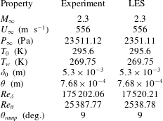
in the far field, impinging on a flat plate turbulent boundary layer. The flow conditions of the experiment (Webb et al.
Reference Webb, Clifford and Samimy2013) and LES are summarized in table 1. For computational accessibility, the simulation Reynolds number is lowered by a factor of 10 from the experimental Reynolds number, by reducing the free stream pressure, while maintaining the free stream velocity, Mach number and boundary layer thickness. This alteration does not contaminate the analysis of desired unsteady features, as also observed in prior studies (Priebe & Martín Reference Priebe and Martín2012; Aubard et al.
Reference Aubard, Gloerfelt and Robinet2013; Morgan et al.
Reference Morgan, Duraisamy, Nguyen, Kawai and Lele2013).
Experimental and computational flow conditions.
An equilibrium turbulent boundary layer is generated through bypass transition of an incoming laminar boundary layer, which is tripped using a counter-flow body force, as discussed by Waindim & Gaitonde (Reference Waindim and Gaitonde2016). The effect is introduced in the simulation as a momentum source term in (2.2). The body force is taken to be uniform in time, so as to avoid low-frequency contamination that can introduce long lasting spurious signatures at the relatively low Reynolds numbers considered. Similarly, the force is assumed homogeneous in the spanwise direction to avoid biasing the development of any particular spanwise wavenumbers.
Concerning boundary conditions, in all cases, a no-slip, zero normal-pressure-gradient wall is used for the wall boundary. The wall temperature is fixed at
 $1.95T_{\infty }$
in the region of the counter-flow body force, to accelerate transition, before returning to an adiabatic state downstream, in which zero normal temperature gradient conditions are enforced, except in the simulations with spatial refinement discussed below, wherein the wall remains adiabatic throughout. The inflow is a specified Blasius boundary layer profile, which is tripped by the counter-flow body force. The shock is imposed at the top boundary through direct specification of the Rankine–Hugoniot conditions. Periodicity is assumed in the spanwise direction, and all other boundary conditions are extrapolated, assuming zero boundary-normal gradients, from the interior. Grid stretching to the downstream and free stream boundaries, in combination with the non-oscillatory spatial scheme, provides for sufficient damping of fluctuations, facilitating the application of these boundary conditions without spurious reflections.
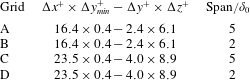
We consider several computational grids (denoted A–D) to ensure that the size of the spanwise domain as well as local grid resolution are adequate, by examining convergence of both mean as well as fluctuating quantities. Details are summarized in table 2. Noting that grid requirements depend on flow parameters as well as numerical scheme resolution, we take our cue from recent published studies. The refined grids (A and B) approach the DNS resolution of previous efforts (Priebe & Martín Reference Priebe and Martín2012), while the standard grids (C and D) are comparable to those in the STBLI LES efforts of Touber & Sandham (Reference Touber and Sandham2009), Agostini et al. (Reference Agostini, Larchevêque, Dupont, Debiève and Dussauge2012), Aubard et al. (Reference Aubard, Gloerfelt and Robinet2013). The grids employed are structured, and spacing in the interaction region is constant in the streamwise (nominal,
 $\unicode[STIX]{x0394}x^{+}=23.5$
; refined,
 $\unicode[STIX]{x0394}x^{+}=16.4$
) and spanwise (nominal,
 $\unicode[STIX]{x0394}z^{+}=8.9$
; refined,
 $\unicode[STIX]{x0394}z^{+}=6.1$
) directions. In the wall-normal direction, hyperbolic tangent growth is applied from the wall (nominal/refined,
 $\unicode[STIX]{x0394}y_{min}^{+}=0.4$
) to the height of the incoming boundary layer (nominal,
 $\unicode[STIX]{x0394}y^{+}=4.0$
; refined,
 $\unicode[STIX]{x0394}y^{+}=2.4$
), above which a power-law spacing is used; the superscript ‘
 $+$
’ denotes normalization with respect to the boundary layer inner variables. To explore the effect of spanwise domain size, the width is varied between
 $2\unicode[STIX]{x1D6FF}_{o}$
(B and D), commonly employed in prior studies (Touber & Sandham Reference Touber and Sandham2009; Agostini et al.
Reference Agostini, Larchevêque, Dupont, Debiève and Dussauge2012; Priebe & Martín Reference Priebe and Martín2012), and
 $5\unicode[STIX]{x1D6FF}_{0}$
(A and C). As shown below, the results indicate that a spanwise domain size of
 $2\unicode[STIX]{x1D6FF}_{0}$
is sufficient. The base flow and perturbations are therefore simulated primarily on grids B and D respectively. It is also evident that the nominal grid (D) adequately reproduces the unsteady characteristics. The longest duration simulations required to analyse the frequency content were therefore performed on grid D.
Computational grid properties.
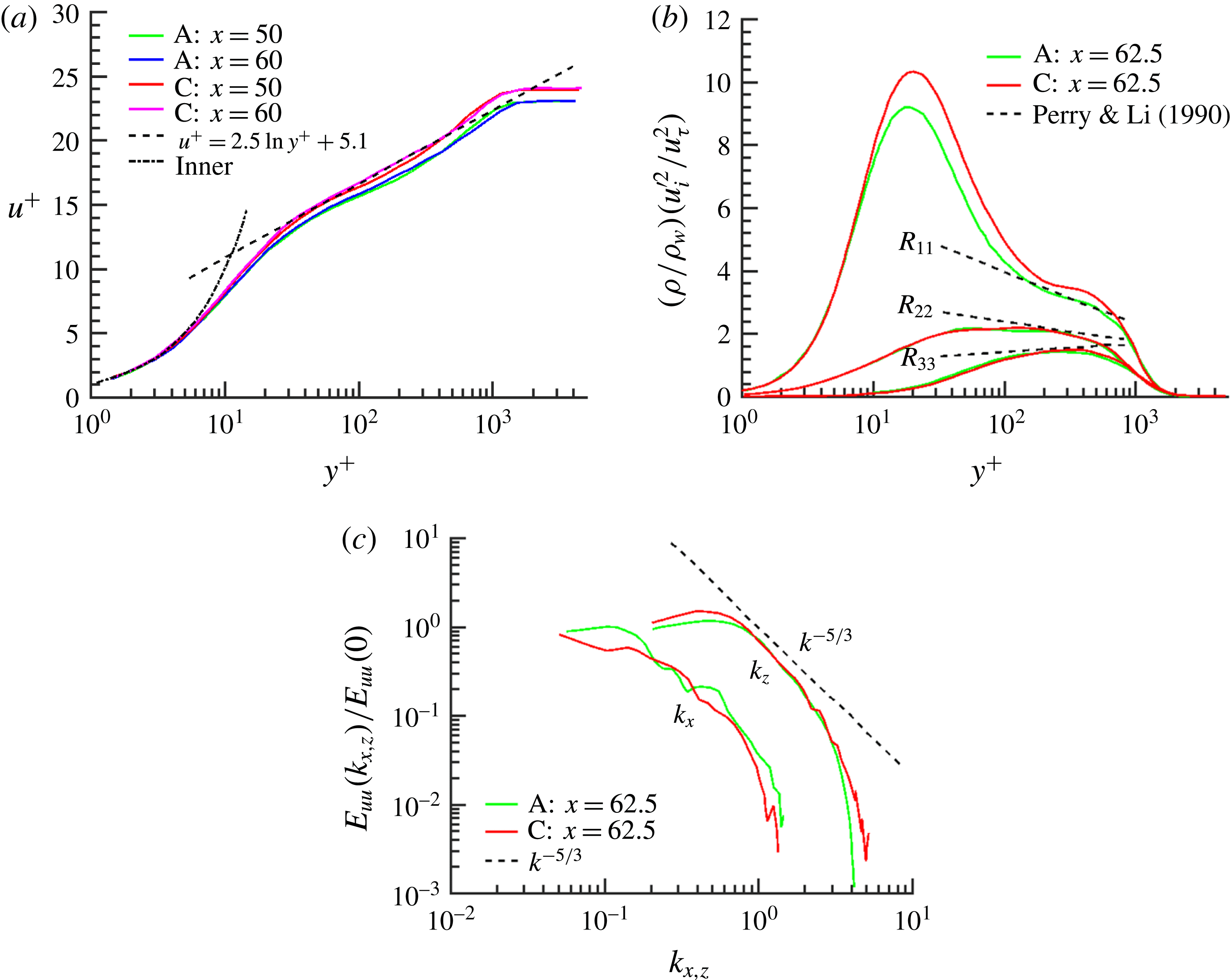
Characteristics of the turbulent boundary layer are presented in figure 1. Turbulence has fully developed by the streamwise region between
 $x/\unicode[STIX]{x1D6FF}_{0}=50$
and
 $x/\unicode[STIX]{x1D6FF}_{0}=65$
, which constitutes the interaction region for the STBLI. Figure 1(a) confirms agreement of the Van Driest transformed velocities with the inner law and log law at various streamwise locations. Note that a consequence of the choice of low Reynolds number is the relative absence of a pronounced wake region (Pirozzoli & Bernardini Reference Pirozzoli and Bernardini2013). This is characteristic of several other efforts in numerical simulation of STBLI (Pirozzoli & Bernardini Reference Pirozzoli and Bernardini2011; Priebe & Martín Reference Priebe and Martín2012; Aubard et al.
Reference Aubard, Gloerfelt and Robinet2013; Morgan et al.
Reference Morgan, Duraisamy, Nguyen, Kawai and Lele2013) and, as shown below, has relatively little influence on the features of the low-frequency phenomena of interest. Figure 1(b) validates the normal Reynolds stresses with analytical results for the outer-scale normal Reynolds stresses given by Perry & Li (Reference Perry and Li1990). Results on grid A are closer to DNS resolution (Pirozzoli, Grasso & Gatski Reference Pirozzoli, Grasso and Gatski2004), and the deviation of the streamwise-normal Reynolds stress with grids C and D is modest. Figure 1(c) presents the one-dimensional energy spectra for streamwise velocity fluctuations near the end of the interaction region. A suitable equilibrium turbulent boundary layer is observed with no low-frequency tones. The spectra further demonstrate the anticipated theoretical rolloff
 $\propto k^{-5/3}$
at high wavenumber and plateau toward low wavenumber as anticipated for one-dimensional (1-D) spectra. The reader is referred to Waindim & Gaitonde (Reference Waindim and Gaitonde2016) for further details regarding properties of the incoming turbulent boundary layer.
Characteristics of the incoming turbulent boundary layer for grids A and C in the region designated for shock impingement, but without the impinging shock, indicate a fully turbulent boundary layer with no spurious low-frequency scales introduced through the bypass transition process. (a) Van Driest transformed streamwise velocity compared with the inner law and log law at
 $x/\unicode[STIX]{x1D6FF}_{0}=50$
and
 $x/\unicode[STIX]{x1D6FF}_{0}=60$
. (b) Normal Reynolds stresses at
 $x/\unicode[STIX]{x1D6FF}_{0}=62.5$
compared with analytical results. (c) Streamwise-normal 1-D energy spectra at
 $x/\unicode[STIX]{x1D6FF}_{0}=62.5$
: components
 $k_{x}$
and
 $k_{z}$
, with reference decay rate.
Time-mean velocity comparison between LES (nominal and refined solutions) and experiment (Webb et al.
Reference Webb, Clifford and Samimy2013). All plots use the same contour set, and spatial coordinates (
 $x$
–
 $y$
plane) are scaled by reference boundary layer thickness,
 $\unicode[STIX]{x1D6FF}_{0}$
. (a) Computational streamwise velocity: refined grid solution (lines) superposed on nominal grid solution (filled). (b) Computational vertical velocity: refined grid solution (lines) superposed on nominal grid solution (filled). (c) Experimental streamwise velocity. (d) Experimental vertical velocity.

A comparison of the time-mean computational and experimental (Webb et al.
Reference Webb, Clifford and Samimy2013) flow fields is presented in figure 2. Figure 2(a,b) shows time-mean contours from the fine grid (B), overlaid on filled contours from the nominal grid (D), to demonstrate a reasonable degree of grid convergence, with the latter grid solution producing a slightly larger time-mean separation. Corresponding particle image velocimetry (PIV) data in the same reference panel and colour map are shown in figure 2(c,d). The boundary layer thickness, interaction length (
 $L_{int}$
, the streamwise distance between the wall-extrapolated reflected and impinging shocks), and point of shock impingement are well matched between the PIV and LES. The experimental data have some contamination due to surface oil flow measurements and an extraneous impinging expansion fan downstream of the interaction. This expansion likely accounts for the flow acceleration and thinner post-reattachment boundary layer observed in the experiment compared with the simulation; the mean flow observed in the simulation is more favourably comparable to studies without this expansion, including those by Piponniau et al. (Reference Piponniau, Dussauge, Debieve and Dupont2009) and Morgan et al. (Reference Morgan, Duraisamy, Nguyen, Kawai and Lele2013). Nonetheless, the key features of the experiment are reproduced faithfully by the simulation. The form of the separated region has a more asymmetric nature in simulation than in experiment. Similar behaviour is observed and discussed by Touber & Sandham (Reference Touber and Sandham2009), concerning a validation study that compares results at identical Reynolds numbers.
STBLI base flow: separation, unsteadiness and comparison with experiment. (a) Time-mean skin friction and wall pressure, with wall pressure point probe locations indicated. (b) Comparison of pre-multiplied wall pressure power spectral density (PSD) at various streamwise locations surrounding the interaction. (c) Comparison of experimental schlieren with isosurface of LES density-gradient magnitude. (d) Reverse flow probability, in coordinates scaled by separation length, demonstrates a moderate degree of flow separation.

The time-mean skin friction and surface pressure profiles in the interaction region are shown in figure 3(a). The interaction region is defined as that between the wall-extrapolated position of the time-mean reflected shock and the shock impingement point, while the separation region is that with negative time-mean streamwise skin friction. The surface pressure does not show a plateau region as is suggested by Délery & Dussauge (Reference Délery and Dussauge2009), since this is a relatively weak interaction, with large unsteady shock displacements compared to separation height. Similar profiles have been reported in other LES (Touber & Sandham Reference Touber and Sandham2009) and DNS (Pirozzoli & Grasso Reference Pirozzoli and Grasso2006). The trend of skin friction is also generally consistent with the previously mentioned studies, though there is quantitative variability of reported skin-friction values in the separation region (Aubard et al. Reference Aubard, Gloerfelt and Robinet2013). Results of the current study most closely resemble the DNS of Pirozzoli & Grasso (Reference Pirozzoli and Grasso2006).
STBLI base flow: instantaneous isosurfaces of the
 $Q$
-criterion coloured by streamwise velocity highlight hairpin vortices. The shocks (in blue) and background shading are indicated by an isosurface and contours of
 $\boldsymbol{u}\boldsymbol{\cdot }\unicode[STIX]{x1D735}p$
.

Surface probe streamwise locations, with normalization by mean separation length
 $(L_{sep})$
, offset by the location of inviscid shock impingement
 $(x_{inv.\;imp.})$
, and reference incoming boundary layer thickness
 $(\unicode[STIX]{x1D6FF}_{0})$
.
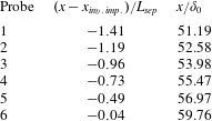
A comparison with experiment of pre-multiplied and normalized wall pressure power spectral density (PSD) at locations described in table 3 and figure 3(a) is shown in figure 3(b). All computational and experimental probe data exhibit low-frequency components. The peak frequency increases moving downstream of the separation point. The most downstream probe is placed in the aft of the recirculation region, where the peak frequency is
 $St_{L}\sim 0.5$
, corresponding primarily to K–H dynamics. Moving upstream, the peak frequency drops and becomes more indicative of the low-frequency
 $(St_{L}\sim 0.03)$
bubble breathing and shock motion. The simulations reproduce the observed trend, with the quantitative agreement becoming better for higher frequencies. Probe placement is exactly reproduced in the simulation with respect to the impinging shock location and experimental probe displacements. As such, discrepancies in comparison of point probe data are primarily due to the difference in separation length between the experiment and simulation. Overall, the results indicate clearly that the simulations capture the key unsteady phenomena observed in the experiment. Comparison with experimental schlieren in figure 3(c) also shows good agreement. Figure 3(d) illustrates the probability of reversed flow in coordinates non-dimensionalized by the mean separation length (
 $L_{sep}$
), with the mean separation point (
 $x_{sep}$
) located at
 $x^{\ast }=0$
:
 $x^{\ast }=(x-x_{sep})/L_{sep}$
. This metric compares well with previous simulations by Agostini et al. (Reference Agostini, Larchevêque, Dupont, Debiève and Dussauge2012) and experiments by Dupont et al. (Reference Dupont, Piponniau, Sidorenko and Debiève2008). Finally, figure 4 shows a three-dimensional instantaneous rendering of the base-flow interaction. In addition to the turbulent boundary layer, which is visualized with an isosurface of the
 $Q$
-criterion coloured by streamwise velocity, the shocks and mid-plane shading are indicated by an isosurface and contours of
 $\boldsymbol{u}\boldsymbol{\cdot }\unicode[STIX]{x1D735}p$
respectively. The mid-plane visualization connects the shock structure with the near-field wave pattern which proceeds periodically downstream from the reflected shock, away from the interaction. The separated flow, the amplification of turbulence through the interaction, and large-scale low-frequency coherent displacement of the reflected shock are dominant features of the interaction.
Forcing cases considered in the present study; case 13 considers a massively separated STBLI with a far-field wedge of
 $11^{\circ }$
to generate the impinging shock.
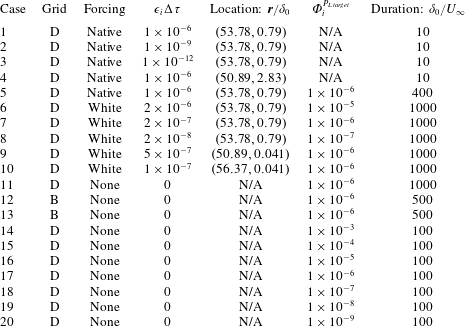
5 Results
5.1 Forcing parameters and cases considered
Numerous simulations were performed to understand numerical and physical aspects of the dynamic linear response of the time-resolved STBLI base flow, using different forcing and constraining parameters as summarized in table 4. Forcing locations are described in terms of their absolute position in the spanwise-normal plane and are periodic in the spanwise direction, encompassing a single line of grid points. However, the forcing itself is non-uniform in the spanwise direction, varying either as a function of the base flow (native, i.e. based on local turbulent fluctuations in the base flow) or randomly (white noise). Furthermore, forcing is applied to all pertinent variables, including mass density, three components of momentum density and energy density. Thus, no bias is introduced regarding two-dimensionality or obliqueness of the perturbations. As indicated in table 4, cases 1–5 rely on native forcing, while cases 6–10 use white-noise forcing, both of which were described earlier in the context of (3.9). Previous work on noise source identification in a turbulent jet relied on the use of native forcing, since the objective was to track existing fluctuations, not to introduce foreign perturbations (Unnikrishnan & Gaitonde Reference Unnikrishnan and Gaitonde2015, Reference Unnikrishnan and Gaitonde2016). However, in this study we observe the base flow to be selective, producing very similar linearly constrained perturbation fields regardless of forcing type, so we choose also to apply random white-noise forcing: this facilitates confirmation of the hypothesis that this selectivity is due to the base flow and not the manner of forcing.
In cases 11–20, the white-noise forcing is turned off after a brief transient of roughly
 $\unicode[STIX]{x1D70F}=5$
, and the simulations are allowed to proceed; this procedure effectively introduces an impulse at
 $\unicode[STIX]{x1D70F}=5$
, from which the simulations proceed without forcing. These cases are designed to highlight the self-sustaining constrained perturbation field due to the presence of the STBLI: the recirculating flow admits much larger perturbation growth rates than the downstream boundary layer, due to constructive feedback through recirculation, and acts to anchor the perturbation field to the interaction region. In contrast, as noted earlier, perturbations introduced in a turbulent boundary layer, without an impinging shock, are convected out of the domain.
5.2 Analysis of transient amplification of unconstrained perturbation field
A study of flow sensitivity to different forcing magnitudes and locations with unconstrained perturbations is performed, employing native forcing with no attenuation. Several forcing locations are considered; the results are distilled with forcing in the boundary layer:
 $(x=53.8,y=0.79)$
(cases 1–3, which differ in forcing magnitude) and free stream:
 $(x=50.9,y=2.83)$
(case 4). Perturbations injected in the boundary layer tend to rapidly decorrelate the base flow and twin flow. To quantify perturbation growth, we discuss the max-norm of the density perturbation field. Figure 5 shows that this norm grows at an exponential rate, regardless of the forcing magnitude. For forcing locations in the boundary layer, this exponential growth begins immediately and eventually plateaus after the perturbation field saturates, at which time the decorrelation between the unperturbed and perturbed states is complete; i.e. the perturbations grow to nonlinear magnitudes. For forcing locations in the free stream, the growth is relatively small until the effects of the perturbation enter the boundary layer, after which it behaves similarly to forcing in the boundary layer.
Evolution of density perturbation field max-norm with time for cases 1–4. A conservative estimate for the linearity threshold, which approximately demarcates the ranges of linear and nonlinear perturbation growth, is indicated near
 $\Vert \unicode[STIX]{x1D731}^{\boldsymbol{P}}\Vert \sim \mathit{O}(10^{-5})$
. Dashed lines representing exponential growth (
 $A/A_{0}=\text{exp}[10.3(\unicode[STIX]{x1D70F}-\unicode[STIX]{x1D70F}_{0})]$
; Lyapunov exponent
 ${\sim}10.3U_{\infty }/\unicode[STIX]{x1D6FF}_{0}$
) are included for reference.
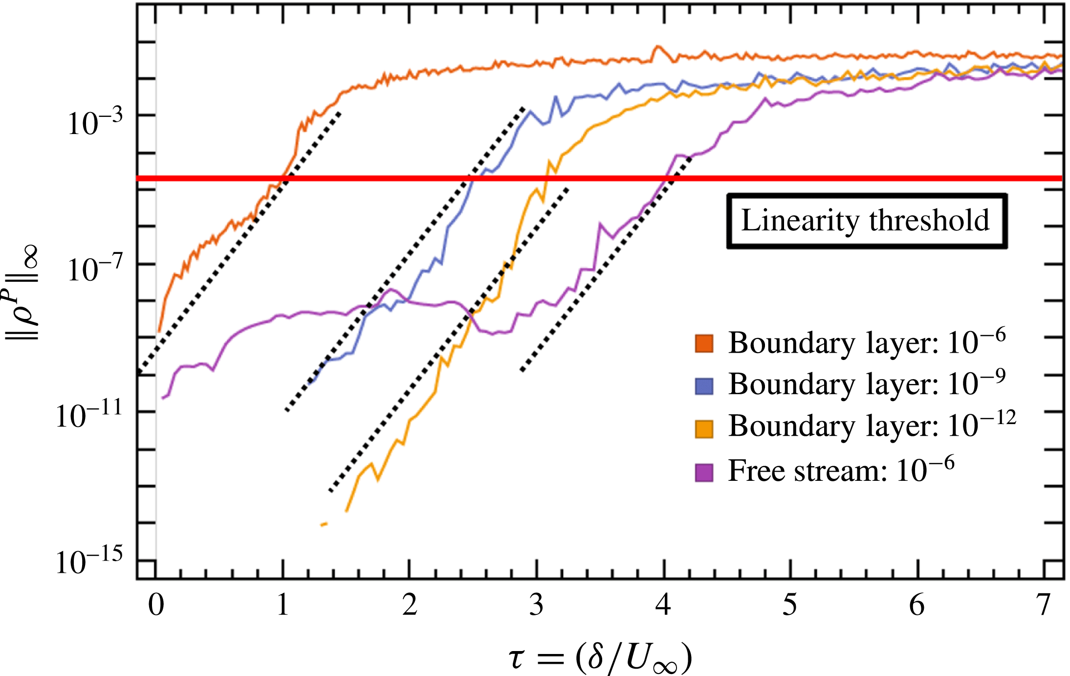
This high sensitivity to perturbation demonstrates the chaotic nature of wall-bounded turbulence. Notably, the exponential nature of non-modal perturbation growth observed for the current unsteady turbulent base flow contrasts with the common observation of non-modal perturbation growth for steady laminar base flows. For example, Matsubara & Alfredsson (Reference Matsubara and Alfredsson2001) discuss the algebraic growth associated with streamwise elongated streaky structures in laminar boundary layers. For high levels of free stream turbulence, this non-modal algebraic growth can occur rapidly and bypass classical modal exponential growth (Tollmien–Schlichting waves), to dominate the early stage of the transition process (Brandt, Schlatter & Henningson Reference Brandt, Schlatter and Henningson2004). However, as figure 5 demonstrates, the current non-modal analysis of the unsteady turbulent environment suggests that exponential growth is naturally recovered in the turbulent regime, consistent with an approximately constant leading Lyapunov exponent for the dynamical system describing the time-resolved turbulent flow.
The growth rates are similar for all forcing scenarios, until the perturbation field amplitude approaches the approximate linearity threshold, above which the assumption that higher-order terms in the expansion of (3.11) are negligible becomes less valid. The linearity threshold is approximate, not definite, and depends on the base flow. For the boundary layer under consideration, nonlinear effects, which are evident in the trajectories of figure 5 as departure from exponential growth, ensue in the range
 $\Vert \unicode[STIX]{x1D731}^{\boldsymbol{P}}\Vert \sim \mathit{O}(10^{-5},10^{-3})$
; a conservative estimate for the linearity threshold is included near
 $\Vert \unicode[STIX]{x1D731}^{\boldsymbol{P}}\Vert \sim \mathit{O}(10^{-5})$
to approximately demarcate the linear and nonlinear ranges of perturbation growth. To ensure perturbations remain linear, the max-norm of the perturbation field should remain much less than the magnitude of the linearity threshold. This is facilitated in § 5.3, by constraining perturbation growth, with
 $\unicode[STIX]{x1D6F7}_{i}^{P_{L\,target}}=10^{-6}<\mathit{O}(10^{-5},10^{-3})$
.
Without constraint, as the perturbations grow larger than the linearity threshold, the growth rate diminishes due to nonlinearity and the perturbation field loses significance, since the twin flow and base flow are now different decorrelated realizations of the STBLI. The two realizations remain statistically similar, but the instantaneous correlation between the two tends toward zero, and the difference between the two can no longer be reasonably interpreted as a perturbation quantity. However, as with many other dynamical systems, the path to nonlinearity can yield useful insight. Information regarding local sensitivity in the boundary layer and the interaction region can be obtained by performing short duration
 $[\mathit{O}(\unicode[STIX]{x1D70F}\sim 1)]$
simulations which remain in the linear regime.
Finally, we note that the time scale for perturbation growth to nonlinear magnitudes in this STBLI is of order
 $\unicode[STIX]{x1D70F}\sim 1$
. In previous studies of a supersonic jet (Unnikrishnan & Gaitonde Reference Unnikrishnan and Gaitonde2016), nonlinear-perturbation magnitudes were not encountered in simulations conducted for much longer duration, indicating the absence of strong feedback mechanisms in the turbulent jet when perturbations are injected in the supersonic flow.
5.3 Analysis of statistically stationary linearly constrained perturbation field
The relevant time scales for low-frequency unsteadiness in the STBLI range from
 $\unicode[STIX]{x1D70F}\sim \mathit{O}(10)$
for Kelvin–Helmholtz phenomena, to
 $\unicode[STIX]{x1D70F}\sim \mathit{O}(200)$
for low-frequency bubble breathing. Since the unconstrained perturbation field grows rapidly to a nonlinear state, to study these time scales in a statistically significant manner we use the method of § 3.3 to constrain the perturbation field to linear magnitudes. In this section we consider cases 5–20, which employ variable attenuation and ensure linearity with respect to the base flow. As discussed in § 3, the interpretation of the constrained perturbation field is not as intuitive, since it effectively results in volume forcing of the linearized Navier–Stokes equations, in a manner that highlights the most dominant growth modes.
5.3.1 Evolution of perturbation field to statistically stationary state
Contours of the vertical velocity perturbation field (
 $v^{P}$
), on a representative spanwise-normal (
 $x$
–
 $y$
) plane, as it evolves to a statistically stationary state (e) in time, superposed with contours of the base-flow pressure field for reference. Perturbations influenced by reflected shock motion and shedding structures in the downstream boundary layer are evident (e). Spatial coordinates are scaled by boundary layer thickness. (a) Shortly after initialization
 $(\unicode[STIX]{x1D70F}=0.05)$
: perturbations localized to forcing location. (b) Before perturbations pass through interaction
 $(\unicode[STIX]{x1D70F}=1.0)$
: relatively isotropic evolution. (c) Immediately after perturbations pass through interaction
 $(\unicode[STIX]{x1D70F}=3.0)$
: non-isotropic evolution. (d) Further in development
 $(\unicode[STIX]{x1D70F}=10)$
: prominent acoustics in near field, amplification begins in interaction. (e) Statistically stationary state
 $(\unicode[STIX]{x1D70F}=50)$
: perturbations highlight the reflected shock and shedding structures downstream of the separation bubble.

The evolution of the vertical velocity perturbation field (case 7) to a statistically stationary state is depicted in figure 6; the base-flow unsteady pressure field is superposed for reference. In the initial stages, the evolution is somewhat isotropic. However, once the perturbations enter the separated region, their evolution becomes more directional in the downstream direction. By panel (c), the outer envelope starts to approximate the reflected shock location. After about
 $10\unicode[STIX]{x1D70F}$
, the perturbations have filled the separated region, and waves with acoustic features are evident downstream. These are also strongly directional, and do not permeate upstream of the reflected shock. Figure 6(e) provides a typical representation of the instantaneous perturbation field under statistically stationary conditions. While the base flow may take many flow-through times to reach statistical stationarity, the perturbations reach stationarity quickly, since they are a very small deviation from the base flow, and their growth is dominated by the absolute instability. The constrained perturbation field is localized to the region just upstream of the reflected shock foot and follows the characteristic along the reflected shock to the far field, demonstrating that with variable attenuation, the perturbation field protrusion upstream is limited. In contrast, for an unconstrained case, the perturbations travel everywhere, including upstream through the subsonic boundary layer, as they grow to nonlinear magnitudes. However, linear-perturbation growth is much stronger in the interaction region and farther downstream than upstream, so these regions of dominant perturbation growth are highlighted when the perturbations are constrained, since weakly growing upstream perturbations are damped relative to strongly growing perturbations in the interaction region and downstream; the magnitude of the latter remain approximately constant due to variable attenuation.
Key features of the statistically stationary perturbation field include convective structures that are shed downstream from the separation region. Additional fine-scale perturbation structures highlight vortices present in the base-flow post-reattachment boundary layer, around which sharp gradients in the flow promote perturbation growth. Also prominent are relatively large magnitude perturbations along the reflected shock wave, demonstrating the influence of perturbation dynamics of the separation region on the reflected shock. Generally, the constrained perturbation field evolves to highlight turbulent features with high potential for linear growth, away from the base flow, which is a novel way to visualize the instantaneous character of a turbulent flow.
Properties of normalized pressure perturbations at a representative location in the post-reattachment boundary layer for different target perturbation magnitudes (cases 14–20). The perturbations are normalized by
 $\unicode[STIX]{x1D6F7}_{\unicode[STIX]{x1D6FC}}^{P_{L\,target}}$
such that collapse of the trajectories demonstrates linearity. (a) Time history of normalized pressure perturbation evolution. Magnified insets demonstrate the minimal cumulative effect of nonlinear error on the trajectories at early and advanced times; this error manifests through slight divergence of the trajectories. (b) Cumulative nonlinear error of each of the trajectories compared to case 19 (
 $\unicode[STIX]{x1D6F7}_{\unicode[STIX]{x1D6FC}}^{P_{L\,target}}=1\times 10^{-8}$
). The error is low-pass filtered to aid in discerning trends. The root-mean-square (r.m.s.) level of the normalized pressure perturbations is included to provide perspective for the error magnitude.

5.3.2 Linearity of constrained perturbation field
Several of the following conclusions rely on the claim that the LC-SLES procedure represents a reasonable approximation for the evolution of constrained linear perturbations as discussed throughout § 3. Notably, any method for propagating linear perturbations through a chaotic nonlinear flow incurs errors that accumulate over time, due to sensitivity of the flow to initial conditions. In this section, we quantify the magnitude of nonlinear errors introduced through the combined effects of the basic SLES procedure (i.e. calculating the evolution of linear perturbations as the difference between two evolving fully nonlinear systems), the variable attenuation procedure, and finite decimal precision: the major contributing causes of nonlinearity. For this purpose, we analyse cases 14–20 that are all initialized with a perturbation impulse taken from a statistically stationary instant of case 11. Each of cases 14–20 proceeds with a distinct perturbation target magnitude, separated by an order of magnitude as described in table 4; the initial impulse for these cases is also scaled with the target perturbation magnitude relative to case 11. Through this premise, linear perturbations would evolve identically in cases 14–20, subject to the relative scaling of the target perturbation magnitude and initial impulse; thus, nonlinear effects may be observed through divergence of the trajectories in time. These simulations evolve for a duration of
 $100\unicode[STIX]{x1D6FF}_{0}/U_{\infty }$
, to observe the accumulation of nonlinearity over a time scale corresponding to the order of low-frequency unsteadiness.
The effects of nonlinearity are described quantitatively in figure 7. Figure 7(a) describes the evolution of pressure perturbations for cases 14–20, at a representative location in the outer layer of the post-reattachment boundary layer; the greatest perturbation magnitudes are observed in this vicinity. The trajectories remain similar over the time window of interest, demonstrating that linearity of the method is maintained. As time progresses, finer-scale features of the signal are distorted for large magnitude perturbations due to accumulation of nonlinearity, as well as for the smallest magnitude perturbation (
 $\unicode[STIX]{x1D6F7}_{\unicode[STIX]{x1D6FC}}^{P_{L\,target}}=1\times 10^{-9}$
) due to lack of decimal precision. Figure 7(b) shows the level of accumulated nonlinear error with time for each case with respect to case 19 (this case has the smallest target perturbation magnitude for which errors due to lack of decimal precision are not evident and is therefore considered to be the most accurate linear solution). The error is low-pass filtered in time to aid in discerning trends between the level of error and the target perturbation magnitude, and the root-mean-square (r.m.s.) level of the normalized pressure perturbations is included to provide perspective for the error magnitude. Concerning cases in which the lack of decimal precision does not introduce error, the errors initially grow from machine precision, with faster growth rates corresponding to larger perturbation target magnitudes, as anticipated. Near
 $\unicode[STIX]{x1D70F}\approx 35$
, an event is encountered which introduces substantial nonlinearity into all perturbations, after which the same trend in growth is recovered. Encouragingly, over the duration of these simulations, the cumulative nonlinear error for the target perturbation magnitude of
 $1\times 10^{-6}$
(employed in cases 5, 7, 9–13, 17) remains less than
 ${\approx}10\,\%$
of the r.m.s. pressure perturbations. Maintaining linearity at this level of precision over such long duration in a chaotic system is not trivial, and these observations attest to the effectiveness of the LC-SLES method.
5.3.3 Time-mean perturbation field and global absolute linear instability
We now discuss the behaviour of the linearly constrained perturbations in the context of a global absolute linear instability. The self-sustaining nature of the perturbations (cases 11–20) indicates the existence of constructive feedback through the recirculation region. This results in large perturbation growth rates in the recirculation region that overwhelm convective growth downstream as well as any additional forcing of the interaction, as discussed further in § 5.3.4. This is consistent with the presence of a global absolute linear instability, as discussed by Chomaz (Reference Chomaz2005). Discussion in this section focuses on the time-mean behaviour of this absolute instability, but it is relevant to note that the time-local behaviour of this absolute instability is not always consistent with its time-mean behaviour, as addressed in § 5.3.6.
The conclusion that self-sustaining constrained perturbations are indicative of a global absolute instability can be confirmed using the framework discussed by Huerre & Monkewitz (Reference Huerre and Monkewitz1990) and Schmid & Henningson (Reference Schmid and Henningson2001) for classifying the nature of instability based on properties of the fundamental solution operator (referred to, in these works, in a less general form: a Green’s function). Since our method is global (Theofilis Reference Theofilis2011) and non-modal (Schmid Reference Schmid2007), including effects from the entire domain, with no restriction on perturbation form, apart from the requirement that they remain linear with respect to the expansion in (3.11), instabilities identified through this method are global and non-modal in nature; the fundamental solution operator propagates the complete global state space (discrete) or global phase space (continuous) in time.
For time-dependent base flows, we generalize the classification of instabilities as follows. Consider the discretized form of (3.7), without forcing and without constraining, which propagates linear perturbations through the flow:
 $$\begin{eqnarray}\displaystyle \unicode[STIX]{x1D6F7}_{i}^{P_{L}}(t)={\mathcal{G}}_{ij}(t,t_{0})\unicode[STIX]{x1D6F7}_{j}^{P_{L}}(t_{0}). & & \displaystyle\end{eqnarray}$$
A flow is classified as globally unstable if
 $$\begin{eqnarray}\displaystyle \limsup _{t\rightarrow \infty }\Vert \boldsymbol{{\mathcal{G}}}(t,t_{0})\Vert _{LN}\rightarrow \infty \quad \text{for some}~t_{0}, & & \displaystyle\end{eqnarray}$$
where
 $\Vert \boldsymbol{{\mathcal{G}}}(t,t_{0})\Vert _{LN}$
is the Lyapunov norm maximized over all initial impulses; conceptually, this is the maximum possible gain of the system represented by (5.1). A globally unstable flow is additionally classified as absolutely unstable if
 $$\begin{eqnarray}\displaystyle \limsup _{t\rightarrow \infty }\frac{\Vert {\mathcal{G}}_{i_{0}j_{0}}(t,t_{0})\Vert _{\infty }}{\Vert \boldsymbol{{\mathcal{G}}}(t,t_{0})\Vert _{LN}}\in (0,1]\quad \text{for some, finite, non-boundary set of}~i_{0},\,j_{0},\,t_{0}.\quad & & \displaystyle\end{eqnarray}$$
A globally unstable flow is additionally classified as convectively unstable if
 $$\begin{eqnarray}\displaystyle \limsup _{t\rightarrow \infty }\frac{\Vert {\mathcal{G}}_{i_{0}j_{0}}(t,t_{0})\Vert _{\infty }}{\Vert \boldsymbol{{\mathcal{G}}}(t,t_{0})\Vert _{LN}}=0\quad \text{for all, finite, non-boundary sets of}~i_{0},\,j_{0},\,t_{0}, & & \displaystyle\end{eqnarray}$$
where
 $i_{0}$
and
 $j_{0}$
represent time-independent indices for the considered degree of freedom, non-boundary sets do not include
 $i_{0}$
on the spatial domain boundary when considering finite domains and
 $t_{0}$
represents the initial time of impulse perturbation to the base flow, which is arbitrary and independent of the other variables;
 $\Vert {\mathcal{G}}_{i_{0}j_{0}}(t,t_{0})\Vert _{\infty }$
represents the max-norm of the fundamental solution operator as a function of the current,
 $t$
, and impulse,
 $t_{0}$
, times, over the finite set of
 $i_{0}$
and
 $j_{0}$
. Naturally, the finite, non-boundary sets of degrees of freedom discussed in (5.3)–(5.4) represent spatially localized regions of the flow. In this sense, equation (5.3) states that the flow is absolutely unstable if the location of maximum perturbation growth is confined to a single local region of the flow. Similarly, equation (5.4) states that the flow is convectively unstable if the location of maximum perturbation growth is not confined to any single local region of the flow. The above use of ‘local’ does not imply the use of any local profile in the analysis, since the full, spatially three-dimensional, ‘global’ flow is analysed. In this context, when perturbation forcing is turned off after an initial impulse, self-sustaining constrained perturbations arise in the STBLI interaction region: the perturbations are perpetually growing, hence the need for constraint, which indicates that the condition,
 $\limsup _{t\rightarrow \infty }\Vert \boldsymbol{{\mathcal{G}}}(t,t_{0})\Vert _{LN}\rightarrow \infty$
, is satisfied for some
 $t_{0}$
, consistent with a global instability. Furthermore, the constrained perturbations, which reveal the most rapid non-modal growth, remain concentrated in the interaction region, which indicates that the condition
 $\limsup _{t\rightarrow \infty }\Vert {\mathcal{G}}_{i_{0}j_{0}}(t,t_{0})\Vert _{\infty }/\Vert \boldsymbol{{\mathcal{G}}}(t,t_{0})\Vert _{LN}\in (0,1]$
is satisfied for some non-boundary set of
 $i_{0}$
,
 $j_{0}$
,
 $t_{0}$
, in which the
 $i_{0}$
correspond to degrees of freedom in the interaction region, consistent with a global absolute instability. (Alternatively, for a turbulent boundary layer, the constrained perturbations are not self-sustaining and convect downstream, indicating that the condition
 $\limsup _{t\rightarrow \infty }\Vert {\mathcal{G}}_{i_{0}j_{0}}(t,t_{0})\Vert _{\infty }/\Vert \boldsymbol{{\mathcal{G}}}(t,t_{0})\Vert _{LN}=0$
is satisfied, for all non-boundary sets of
 $i_{0}$
,
 $j_{0}$
,
 $t_{0}$
, consistent with a global convective instability.)
Filled contours of the time-mean linearly constrained streamwise velocity perturbation superposed with contours of the time-mean base-flow pressure field for reference. The time-mean perturbation field is consistent with a time-mean linear tendency (time-mean behaviour of the absolute instability in the unsteady environment) for upstream motion of the reflected shock. All plots have the same contour levels and spatial coordinates (
 $x$
–
 $y$
plane) scaled by boundary layer thickness. (a) Case 11: nominal grid (D) with
 $9^{\circ }$
shock generator, moderately separated interaction. (b) Case 12: refined grid (B), spanwise averaged, with
 $9^{\circ }$
shock generator, moderately separated interaction. (c) Case 13: refined grid (B), spanwise averaged, with
 $11^{\circ }$
shock generator, massively separated interaction. (d) Schematic describing how the time-mean perturbations indicate a time-mean linear tendency for upstream motion of reflected shock. Notably, the distinction between the twin-flow and base-flow shocks in the mean is spatially diffuse due to base-flow unsteadiness.

We can quantify the effect of this global absolute instability in the STBLI by examining the time mean of the self-sustaining linearly constrained perturbation field,
 $\overline{\unicode[STIX]{x1D731}^{\boldsymbol{P}}}$
, which we designate as the time-mean linear tendency of the base flow. We interpret the non-zero time-mean linear tendency as the time-mean behaviour of the absolute instability in the unsteady environment. This is clarified by noting that the time mean of the perturbation field between two statistically identical turbulent realizations (twin and base) will tend toward zero with time. However, for this STBLI, the absolute instability present in the base flow manifests as a time-mean linearly constrained perturbation field that does not tend toward zero with time, since the instability biases linear-perturbation growth in the unsteady environment. Indeed, as noted earlier, the constraints of § 3.3 effectively highlight this absolute instability at the expense of other more weakly growing (convective) instabilities, which are damped. Since the twin-flow simulation solves the forced and linearly constrained Navier–Stokes equations, it represents a linear departure from the base-flow simulation. As such, their time means (twin and base) can be slightly different – the magnitude of the difference being determined by the perturbation target magnitude (
 $\unicode[STIX]{x1D6F7}_{\unicode[STIX]{x1D6FC}}^{P_{L\,target}}$
) – and is reflective of the time-mean behaviour of the underlying absolute instability. The underlying bias in linear-perturbation growth in the unsteady environment, leading to a non-zero time-mean linear tendency, can be thought of as analogous to an unstable zero-frequency (non-oscillatory) mode, which can be found in global IVP and EVP analyses of steady base flows that do not satisfy the steady Navier–Stokes equations, including time-mean STBLIs (Touber & Sandham Reference Touber and Sandham2009; Pirozzoli et al.
Reference Pirozzoli, Larsson, Nichols, Bernardini, Morgan and Lele2010; Waindim et al.
Reference Waindim, Bhaumik and Gaitonde2016; Nichols et al.
Reference Nichols, Larsson, Bernardini and Pirozzoli2017).
The time-mean linear tendency is described in figure 8, visualized by the time-mean streamwise velocity perturbation, for cases 11–13, in panels (a–c) respectively. We note that the mean perturbation field converges at a much slower rate than the mean base flow, since the range of the perturbation field extends several orders of magnitude. Thus, convergence of the mean is sensitive to the behaviour of large magnitude perturbations. As such, discrepancies between the nominal (a) and refined (b) grids are expected and observed, and they are attributable not only to differences in spatial refinement, but also to differences in initial STBLI realizations between different cases. Sensitivity to averaging duration can also occur, even with sufficiently long duration simulations which allow for accurate convergence of the time-mean flow field; results on the nominal grid (a) are best converged in this sense, since case 11 has the longest simulation duration. This comparison also provides an indication of the level of uncertainty in the time-mean perturbation quantities and sensitivity of these quantities to the base flow. Nonetheless, all cases, including the interaction with stronger separation (c, case 13), exhibit similar time-mean linear tendencies, with equivalent physical significance.
The time-mean behaviour of the absolute instability depicted in figure 8 is clarified by noting that, for all cases, in the time-mean sense, the reflected shock position observed in the linearly constrained twin flow is upstream from its position in the base flow. This results in a negative time-mean streamwise velocity perturbation in the region of the reflected shock as illustrated in figure 8(d); i.e. the mean linearized shock position is not coincident with the mean shock position, but is rather located slightly upstream. Notably, the unsteadiness of the base flow inhibits a sharp indication of the position of the linearized and base-flow shocks in the mean, since the difference in position between the shocks, at any given instant, is determined by the perturbation target magnitude,
 $\mathit{O}(10^{-6})$
, which is certainly much less than the magnitude of unsteady shock displacement in the base flow,
 $\mathit{O}(1)$
; however, the spatially diffuse negative time-mean streamwise velocity perturbation in the region of the spatially diffuse time-mean reflected shock reveals this behaviour. In conjunction with the time-local analysis of § 5.3.6, we can furthermore conclude, regarding low-frequency motion, that when the reflected shock is located near its mean position, the corresponding time-local linear tendency promotes upstream shock motion, increasing the size of the separation region, consistent with the observed time-mean linear tendency of the interaction. These findings are not inconsistent with those of Touber & Sandham (Reference Touber and Sandham2009), Pirozzoli et al. (Reference Pirozzoli, Larsson, Nichols, Bernardini, Morgan and Lele2010) and Nichols et al. (Reference Nichols, Larsson, Bernardini and Pirozzoli2017), who employ the time-mean base flow to describe a linearly unstable non-oscillatory global mode. However, the current analysis shows that the tendency for upstream motion is definite; there is not an arbitrary nature to the sign (direction) of the absolute instability, it is not symmetric as suggested in previous modal mean-flow analyses, and this observation has physical significance. Indeed, the current findings are consistent with the asymmetry of shock motion discussed by Piponniau et al. (Reference Piponniau, Dussauge, Debieve and Dupont2009), in which upstream motion occurs more rapidly than downstream motion. We discuss this in detail in § 5.3.5, followed by an analysis of how this absolute instability interacts with the nonlinear nature of the base flow in § 5.3.6.
We conclude this section by postulating that for any flow admitting a global absolute linear instability, the time-mean linear tendency of the unsteady turbulent base flow should be qualitatively consistent with traditional stability analyses applied to the time-mean turbulent flow. This postulate is confirmed in the current case of the STBLI, since the time-mean linear tendency is consistent with the behaviour of the absolutely unstable, non-oscillatory, global mode of the time-mean STBLI. Compared to stability analyses of the time-mean turbulent flow, however, the dynamic linear response yields additional insight into the underlying mechanisms that sustain the unsteadiness, particularly in addressing time-local perturbation dynamics, as discussed in § 5.3.6.
Contours of root-mean-square vertical velocity perturbations (
 $v_{rms}^{P}$
) for cases 7 and 9–11, subject to external forcing at different locations, superposed with mean pressure contours of the base flow for reference. All plots have the same contour levels and spatial coordinates (
 $x$
–
 $y$
plane) scaled by boundary layer thickness. (a) Case 7: stochastic forcing in separated shear layer; location,
 $(53.78,0.79)$
. (b) Case 9: stochastic forcing in upstream subsonic boundary layer; location,
 $(50.89,0.041)$
. (c) Case 10: stochastic forcing in recirculation region; location,
 $(56.37,0.041)$
. (d) Case 11: self-sustaining with no forcing; most similar to forcing in recirculation region (case 10).
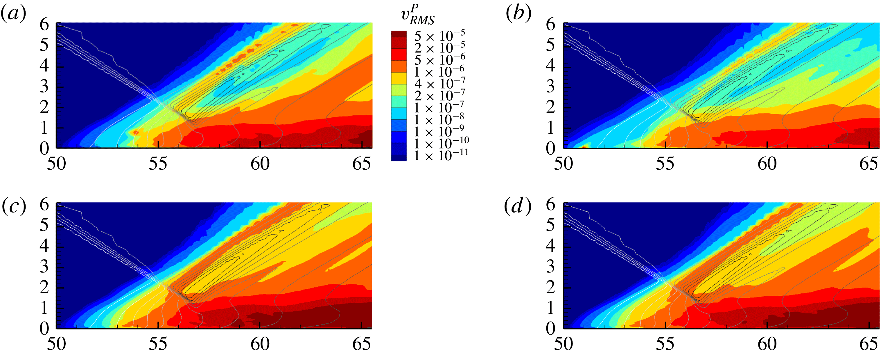
5.3.4 Effects of stochastic forcing on perturbation field
The linearly constrained perturbation field of the STBLI shows relatively small sensitivity to the specific nature of forcing, as anticipated given the absolute nature of the instability. Results with stochastic forcing are therefore similar to those shown earlier. This is consistent with the discussion by Chomaz (Reference Chomaz2005): in absolutely unstable flows, the internal growth of perturbations overshadows the response to external forcing. On the other hand, the linearly constrained perturbation field of the turbulent boundary layer, without an impinging shock, requires continuous stochastic forcing to sustain its convectively unstable perturbation field, consistent with the common understanding (Chomaz Reference Chomaz2005).
To demonstrate the selective nature of the STBLI perturbation field, the effects of forcing location on the root-mean-square (r.m.s.) vertical velocity perturbation fields are displayed in figure 9. Apart from a local area of influence around each forcing location, the character of the perturbation field is very similar between the different cases. For instance in case 9, the forcing location provides a perturbation source upstream, but these perturbations are attenuated relatively quickly, and the major area of perturbation activity remains in the separation region and downstream boundary layer. Likewise, for case 7, the forcing effects are localized to the separated shear layer. For case 10, in which a perturbation source is added in the recirculation region, the results are quite similar to case 11, containing no forcing. This suggests that the self-sustaining perturbation field of case 11 is akin to a perturbation source originating in the recirculation region; i.e. the absolute instability is sustained by internal perturbation growth within the recirculation region. Additionally, it demonstrates that the STBLI is more sensitive to perturbations in the recirculation region than the upstream region; i.e. all attempts to stochastically force perturbations outside of the recirculation region are overshadowed by unforced perturbation growth in the recirculation region. These observations support the finding that the absolute instability is sustained by constructive feedback through the recirculation region and is not receptive to external forcing. The self-sustaining perturbation field, driven by the absolute instability, is the most natural perturbation field to analyse, since it removes any arbitrariness due to the presence of forcing, and is therefore the subject of much of the analysis below.
5.3.5 Spectral content of base-flow and perturbation fields
We now analyse the unsteady dynamics of the base-flow and perturbation fields using several different time series. These series are chosen to describe a variety of unsteady features: the shock footprint indicated by wall pressure fluctuations, indicators of the size of the separation bubble, as well as the near-field shock location. Observations of the base flow are first summarized to provide a foundation for the subsequent discussion of the accompanying perturbation dynamics. Overall, the dynamics of the base flow agrees well with those described in the literature, providing a measure of base-flow validation necessary for the perturbation analysis. The discussion focuses on several prominent frequency bands, each described qualitatively with a corresponding physical process: low-frequency content
 $(St_{L}\sim 0.03)$
, corresponding to separation bubble breathing and large-scale shock motion, low–mid-frequency content
 $(St_{L}\sim 0.1)$
, corresponding to bubble oscillations, high–mid-frequency content
 $(St_{L}\sim 0.5)$
, corresponding to Kelvin–Helmholtz induced shear layer phenomena, including shedding and flapping of the reflected shock and high-frequency
 $(St_{L}\gtrsim 1)$
jitter, corresponding to the passage of fine-scale turbulent fluctuations.
In all cases, the time series are sampled at intervals of
 $20\unicode[STIX]{x1D6FF}_{0}/U_{\infty }$
, and the power spectral density (PSD) is obtained using Welch’s windowed overlapping segments estimator method, by splitting the signal into eight segments with 50 % overlap and windowing with the Hamming function. The PSD is pre-multiplied by the corresponding Strouhal number, based on the time-mean separation length, to effectively represent the power distribution on a logarithmic scale. Further, the PSD is normalized, such that the integral of pre-multiplied power over all resolved frequencies is unity. In some cases, the PSD is filtered using Konno–Ohmachi (KO) smoothing, which ensures constant bandwidth smoothing on a logarithmic scale (Konno & Ohmachi Reference Konno and Ohmachi1998). The base-flow and perturbation fields were evaluated, in multiple simulations, for over five cycles of the low-frequency
 $(St_{L}\sim 0.03)$
unsteadiness. For the former, adequacy was established by comparing with the known spectra from well-documented results for this configuration (Dupont et al.
Reference Dupont, Haddad and Debiève2006; Touber & Sandham Reference Touber and Sandham2009; Aubard et al.
Reference Aubard, Gloerfelt and Robinet2013). With regard to the perturbations, these reach statistical stationarity quickly, and short duration simulations are observed to be adequate to describe their time-local behaviour. For example, in principle, the band-isolation study (§ 5.3.6) only requires one cycle of the low-frequency unsteadiness; results were nonetheless confirmed by comparing with the full data set. Therefore, the resolution of low-frequency unsteadiness is reasonable to support the conclusions drawn in this work.
Base-flow reflected shock location, reverse flow mass-per-span and separation bubble mass-per-span signals, with corresponding power spectral densities. (a) Base flow: reflected shock location signal, with evident asymmetry. Positive location corresponds to upstream displacement from the time-mean position. Displacement is normalized by the time-mean separation length. (b) Base flow: reverse flow mass-per-span signal, with time-mean subtracted. (c) Base flow: separation bubble mass-per-span signal, for flow satisfying
 $u<0.15u_{\infty }$
, with time-mean subtracted. (d) Pre-multiplied and normalized power spectral densities comparing base-flow shock location, reverse flow and separation bubble mass-per-span signals.

Notably, asymmetry is observed in the shock motion, whereby large-displacement upstream motion occurs relatively quickly, followed by slower, less coherent, downstream motion, at intervals representative of the low-frequency
 $(St_{L}\sim 0.03)$
cycle. This is evident in the base-flow near-field reflected shock location signal (figure 10
a), which describes the streamwise location of the maximum value of velocity dotted with pressure gradient (constrained to the near-field region of the reflected shock), at a height of
 $y=4\unicode[STIX]{x1D6FF}_{0}$
, in the spanwise centre of the domain. As noted earlier, this asymmetry is consistent with the experimental observations of Piponniau et al. (Reference Piponniau, Dussauge, Debieve and Dupont2009). Further analysis of the genesis of this asymmetry is provided in § 5.3.6.
Two additional signals are analysed to elucidate the dynamics of the separation region. A reverse flow mass-per-span signal, comprising the total fluid mass per span in the reversed flow region, is presented in figure 10(b), and a separation bubble mass-per-span signal, of the total fluid mass per span satisfying
 $u<0.15u_{\infty }$
, is presented in figure 10(c). The reverse flow mass-per-span signal (figure 10
b) is dominated by
 $St_{L}\sim 0.1$
content, corresponding to bubble oscillations, with a minor side lobe at
 $St_{L}\sim 0.03$
, corresponding to low-frequency bubble breathing. On the other hand, the separation bubble mass-per-span signal:
 $u<0.15u_{\infty }$
(figure 10
c) shows a smaller contribution from
 $St_{L}\sim 0.1$
content, and a larger contribution from
 $St_{L}\sim 0.03$
content, resulting in a better indication of shock displacement. This trend holds across other thresholds defining the ‘turbulent separation bubble’: larger thresholds on streamwise velocity result in a better indication of low-frequency
 $(St_{L}\sim 0.03)$
large-scale shock motion, while smaller thresholds result in a better indication of low–mid-frequency
 $(St_{L}\sim 0.1)$
bubble oscillation dynamics. As § 5.3.6 elaborates, the dynamics in these separate frequency bands can be described relatively independently. Priebe & Martín (Reference Priebe and Martín2012) similarly observe significant
 $St_{L}\sim 0.1$
content corresponding to streamwise oscillation of the low-pass filtered separation point in the DNS of a Mach 2.9 compression ramp STBLI. In fact,
 $St_{L}\sim 0.1$
content is found in the separation region power spectra of many studies (Dupont et al.
Reference Dupont, Haddad and Debiève2006; Touber & Sandham Reference Touber and Sandham2009; Aubard et al.
Reference Aubard, Gloerfelt and Robinet2013), but it is often not discussed in detail.
Comparison of base flow and perturbation wall pressure power spectral densities at streamwise locations surrounding the interaction region. The Strouhal number is based on the incoming free stream velocity and the mean separation length. Streamwise distance has been normalized by the mean separation length, and the mean separation point is located at
 $x^{\ast }=0$
. Spectrum normalization is performed independently at each streamwise location. (a) Base-flow wall pressure pre-multiplied and normalized power spectral density. (b) Perturbation wall pressure pre-multiplied and normalized power spectral density.
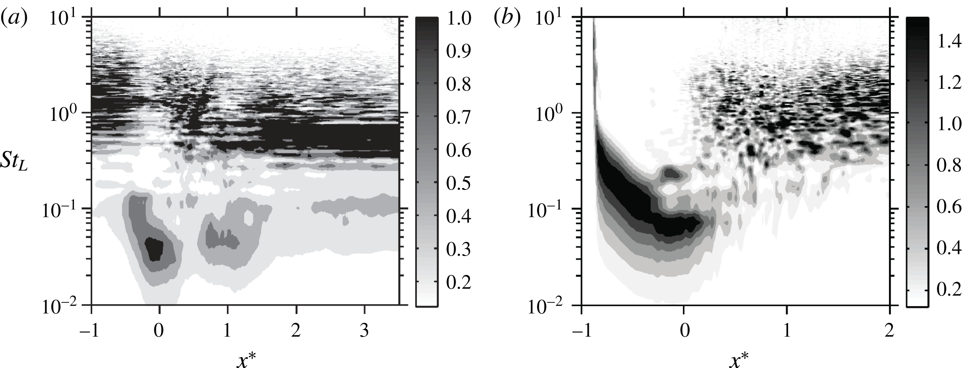
We also observe a significant lagged correlation between the reflected shock motion and the dynamics of the separation bubble. The maximum correlation coefficient between the shock location and the reverse flow mass-per-span signals is 0.38 with a lag of
 $18\unicode[STIX]{x1D70F}$
. A stronger instantaneous correlation of 0.53 is found with a lag of
 $15\unicode[STIX]{x1D70F}$
, when correlating the shock location and separation bubble mass-per-span:
 $u<0.15u_{\infty }$
signals. These correlations of shock motion with the size of the separation, in which the shock motion lags in response to changes in separation, are consistent with previous observations by Morgan et al. (Reference Morgan, Duraisamy, Nguyen, Kawai and Lele2013), confirming that a causal relationship could exist, whereby large-scale shock motion responds primarily to growth or contraction of the separation bubble. This causal relationship (sign of the lag) is independent of the height at which the correlation with the reflected shock is taken, though the magnitude of the correlation and lag vary.
In figure 11, the base flow and perturbation wall pressure PSDs are compared at streamwise locations around the interaction region. The PSD at each streamwise location is normalized, such that the integral of pre-multiplied power over all resolvable frequencies is unity. The base-flow wall pressure dynamics agree well with previous studies (Dupont et al.
Reference Dupont, Haddad and Debiève2006; Touber & Sandham Reference Touber and Sandham2009; Agostini et al.
Reference Agostini, Larchevêque, Dupont, Debiève and Dussauge2012; Aubard et al.
Reference Aubard, Gloerfelt and Robinet2013). Low-frequency content
 $(St_{L}\sim 0.03)$
, corresponding to shock motion and bubble breathing, is prominent near the time-mean separation and reattachment locations; normalizing the PSD independently at each streamwise location facilitates the identification of prominent low-frequency dynamics at reattachment; these fluctuations are less intense than the low-frequency fluctuations at separation, but they are intense compared to the pressure fluctuations across the full spectrum at reattachment. Low–mid-frequency content
 $(St_{L}\sim 0.1)$
, corresponding to bubble oscillations, is present near the separation and reattachment points, as well as downstream of the interaction region. High–mid-frequency content
 $(St_{L}\sim 0.5)$
, corresponding to Kelvin–Helmholtz shedding, is present downstream of the interaction region. High-frequency content
 $(St_{L}\gtrsim 1)$
, typical of fine-scale features in a turbulent boundary layer, is prominent upstream of the interaction region; it persists throughout the interaction, reducing in frequency as its convective speed slows and its outer scale increases, eventually being overtaken in amplitude by a dominant contribution from
 $(St_{L}\sim 0.5)$
shed structures downstream of the interaction.
Necessarily, the unsteady dynamics in each of these frequency bands will not collapse with
 $St_{L}=fL/U_{\infty }$
for all flow conditions. Rather,
 $St_{L}$
is chosen to describe the unsteadiness since the prominent low-frequency unsteadiness collapses with this Strouhal number for a variety of flow conditions (Dussauge et al.
Reference Dussauge, Dupont and Debiève2006), providing a unified scale on which to compare all of the described bands with respect to the low-frequency unsteadiness for these particular flow conditions. Indeed, the high-frequency band associated with fine-scale turbulent fluctuations of the incoming boundary layer must collapse with
 $St_{\unicode[STIX]{x1D6FF}}=f\unicode[STIX]{x1D6FF}_{0}/U_{\infty }=1$
, independent of the STBLI separation length. It is still to be determined for which Strouhal numbers the two described mid-frequency bands might collapse, since these frequency bands have not been characterized in as extensive detail in many studies.
The wall pressure PSD for the perturbation field is calculated in the same manner as for the base flow. Downstream of the interaction, high frequencies typical of a turbulent boundary layer
 $(St_{L}\gtrsim 1)$
are identified, consistent with the observation that the perturbation field highlights regions of high-potential linear growth of the base-flow turbulent structures. Mid-frequency
 $(St_{L}\sim 0.06-0.1)$
content is found near the time-mean separation point, corresponding to perturbations of the reflected shock. This suggests that changes in the linear tendency of the reflected shock are more significantly influenced by mid-frequency mechanisms than low-frequency mechanisms. The wall pressure perturbation PSD upstream of the time-mean separation point requires special care in its interpretation, since the perturbation field does not always penetrate much upstream of the time-mean separation point. For instance, if a particular upstream low-frequency motion of the reflected shock does not reach its greatest upstream extent, the perturbation field will also not be carried farther upstream. The effect of this is to skew the PSD toward higher frequencies. Nonetheless, this analysis illustrates that while the perturbation field is a strong function of the base flow, there are significant differences in the spectral properties of the base-flow and perturbation fields.
To demonstrate the linearity of forcing and attenuation on perturbation field spectral content, wall pressure spectra are presented in figure 12, for cases 6–8, in which forcing and attenuation are applied with different magnitudes, separated by one order of magnitude, as described in table 4. In these spectra, the PSD is normalized by
 $(\unicode[STIX]{x1D6F7}_{\unicode[STIX]{x1D6FC}}^{P_{L\,target}})^{2}$
, under which the spectra should collapse if linearity is maintained. KO smoothing has been applied to reduce noise at higher frequencies. At the time-mean separation point (a), cases 7 and 8 collapse, while case 6 undershoots the peak. The collapse of cases 7 and 8 is anticipated; however, the deviation of case 6 appears to demonstrate nonlinearity in the scaling of forcing and attenuation target magnitudes between cases. This apparent nonlinearity can result from differences in the specific realization of stochastic forcing, which is unique to each case; it is not indicative that higher-order terms in the expansion of (3.11) are non-negligible, since the results § 5.3.2 demonstrate that the scaling of attenuation alone is linear. Similarly, the results of Unnikrishnan & Gaitonde (Reference Unnikrishnan and Gaitonde2016) demonstrate that the method is linear with respect to scaling of deterministic forcing. Regardless, at the downstream location (b), all cases collapse indicating linearity. The results presented herein regarding the self-sustaining linearly constrained perturbation field are obtained with the attenuation factor of case 7, reaffirming that the perturbations remain linear with respect to the base flow.
Wall pressure perturbation power spectral densities demonstrating the linearity of forcing and attenuation for cases 6–8. The PSDs have been normalized by
 $(\unicode[STIX]{x1D6F7}_{\unicode[STIX]{x1D6FC}}^{P_{L\,target}})^{2}$
to demonstrate collapse of the spectra. (a) Wall pressure perturbation power spectral density at the time-mean separation point. (b) Wall pressure perturbation power spectral density downstream of the reattachment point
 $(x^{\ast }=1.1)$
.
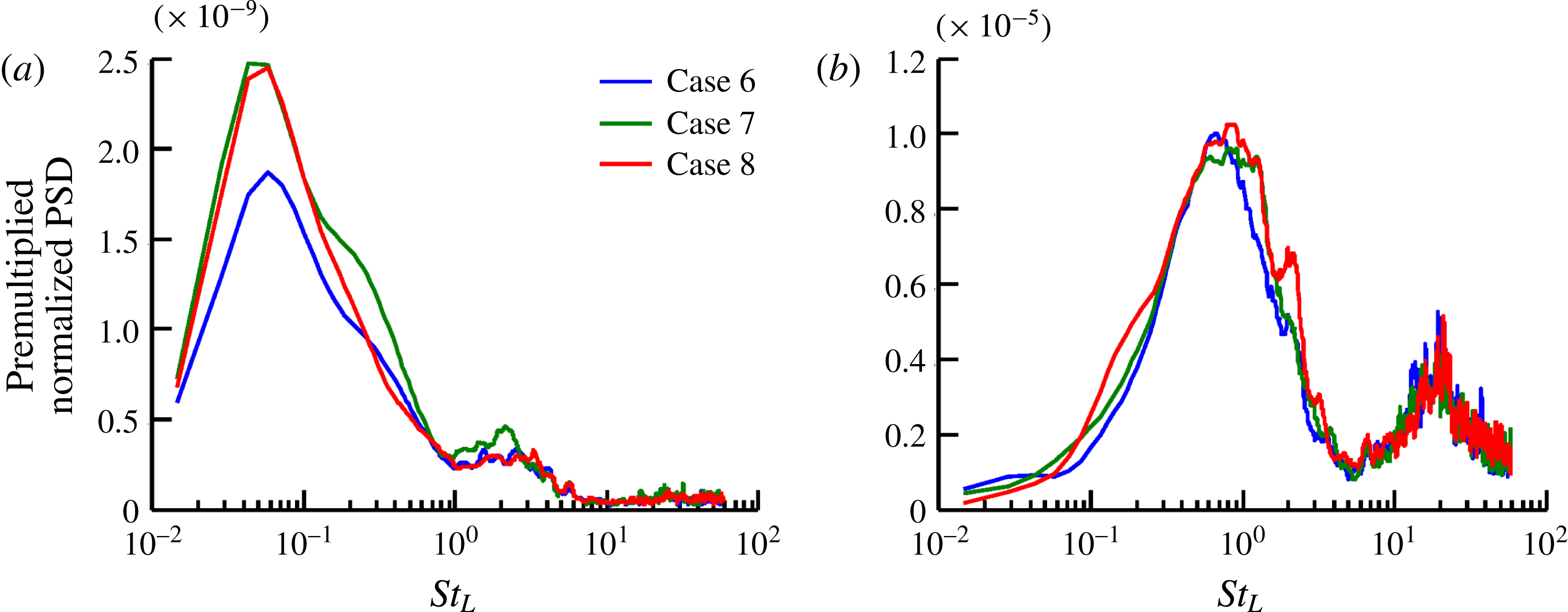
The attenuation factor is related to the enforcement of linearity and thus provides insight into the dynamics of the interaction, since it distinguishes instances in time where perturbation growth is more prominent from those where it is less so. Characteristics of the variable attenuation factor for the self-sustaining perturbation field (case 11) are presented in figure 13. The attenuation-factor PSD is characterized by two peaks at approximately
 $St_{L}\sim 1$
, corresponding to the passage of convecting fine-scale turbulent structures, and
 $St_{L}\sim 200$
, corresponding to the changing location of the maximum norm of the perturbation field
 $(\unicode[STIX]{x1D6F7}_{\unicode[STIX]{x1D6FC}}^{P})$
with the fine-scale features of convecting structures; recall, the perturbation field evolves to highlight turbulent features with high potential for linear growth. Scrutiny of animations of the evolving perturbation and base-flow fields indicates that the maximum norm of the perturbation field
 $(\unicode[STIX]{x1D6F7}_{\unicode[STIX]{x1D6FC}}^{P})$
is often associated with a hairpin-like structure downstream of the interaction region. Since the attenuation factor,
 $\unicode[STIX]{x1D6FC}$
, is directly dependent on
 $\unicode[STIX]{x1D6F7}_{\unicode[STIX]{x1D6FC}}^{P}$
, it varies with the coherence time of these turbulent structures, explaining the low-frequency peak. Additionally, the band of frequencies comprising this peak indicates that high-frequency
 $(St_{L}\sim 1)$
turbulent content and high–mid-frequency
 $(St_{L}\sim 0.1{-}0.5)$
content have a much stronger tendency for linear growth in the base-flow turbulent environment than low-frequency
 $(St_{L}\sim 0.03)$
content. It follows that any mechanism for instability acting over low-frequency scales must have a much smaller growth rate than its higher-frequency
 $(St_{L}\sim 0.1{-}2)$
counterparts. The high-frequency
 $(St_{L}\sim 200)$
peak corresponds to variation of
 $\unicode[STIX]{x1D6F7}_{\unicode[STIX]{x1D6FC}}^{P}$
with short-time evolution of fine-scale features on a passing coherent structure. Since the turbulent structure evolves throughout its time of coherence, the spatial location at which
 $\unicode[STIX]{x1D6F7}_{\unicode[STIX]{x1D6FC}}^{P}$
is found will vary with the evolution of that turbulent structure as the location for maximum potential growth changes. The attenuation factor is smoothly resolved by the chosen time step, with the high-frequency variation of
 $\unicode[STIX]{x1D6F7}_{\unicode[STIX]{x1D6FC}}^{P}$
being resolved by
 $\mathit{O}(10)$
time steps. Note that the discrete attenuation factor
 $(1-\unicode[STIX]{x1D6FC}\unicode[STIX]{x0394}\unicode[STIX]{x1D70F})$
exceeds unity in some instances, leading to brief amplification of the perturbation field. On average, however, the discrete attenuation factor takes a value of 0.860, with a standard deviation of 0.084. It follows that, on average, the absolute instability of the STBLI corresponds to a Lyapunov exponent of approximately
 $140U_{\infty }/\unicode[STIX]{x1D6FF}_{0}$
, significantly larger than the Lyapunov exponent of
 $10.3U_{\infty }/\unicode[STIX]{x1D6FF}_{0}$
identified earlier for the shock-free turbulent boundary layer; i.e. the STBLI absolute instability results in an exponential rate of perturbation amplification that is an order of magnitude larger than the shock-free, convectively unstable, turbulent boundary layer.
Discrete variable attenuation-factor signal and power spectral density for the self-sustaining perturbations of case 11. (a) Discrete variable attenuation-factor signal:
 $1-\unicode[STIX]{x1D6FC}\unicode[STIX]{x0394}\unicode[STIX]{x1D70F}$
. (b) Pre-multiplied and normalized power spectral density of discrete variable attenuation factor.
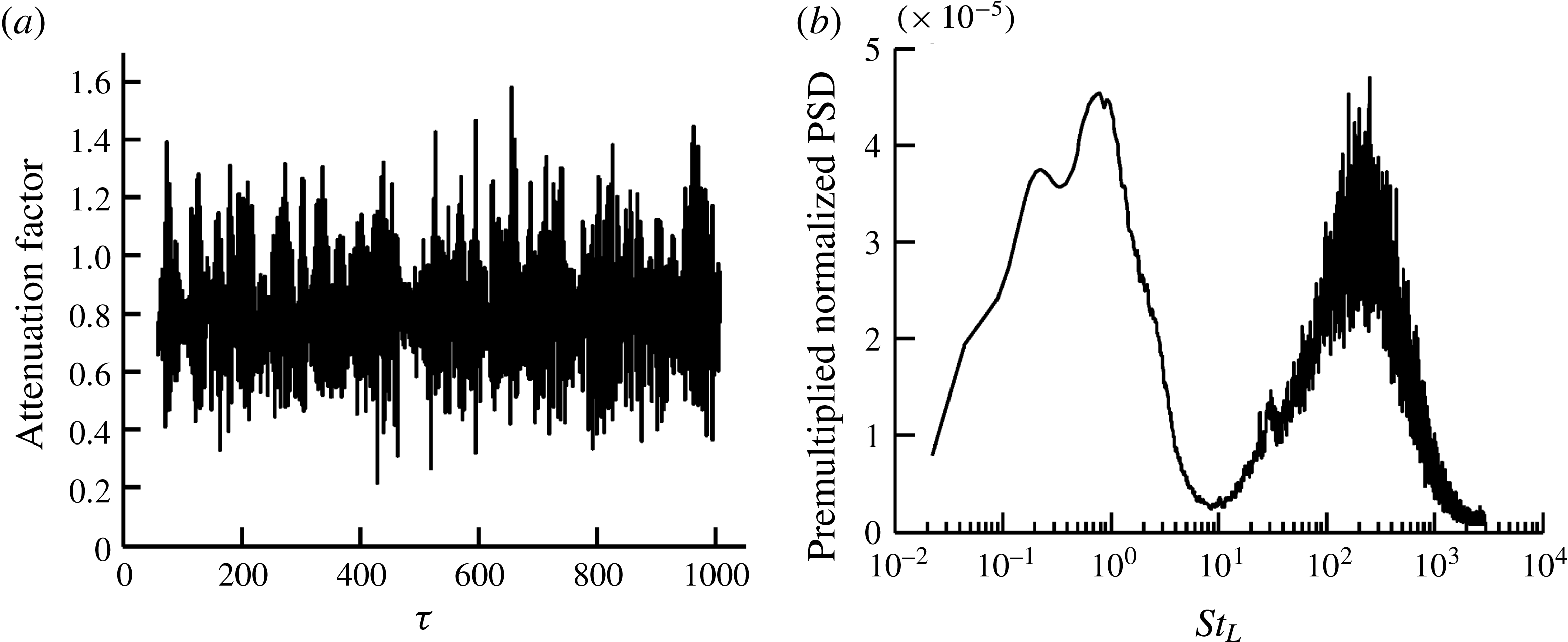
5.3.6 Band isolation of base-flow and perturbation fields
In this section, we isolate the flow characteristics associated with the prominent frequency bands observed in the spectral analysis of § 5.3.5. For this purpose, a series of low-pass finite-impulse-response (FIR) window-based filters are applied. Since the low-frequency dynamics are broadband, a sharp cutoff is neither necessary nor desirable. They are therefore implemented through a time domain moving average filter, to optimize smoothing characteristics in the time domain, albeit with a wider transition band. The first low-pass cutoff is chosen at
 $St_{L}=0.06$
, to isolate low-frequency unsteadiness of bubble breathing around
 $St_{L}\sim 0.03$
. The low-pass content is then subtracted from the instantaneous signal, and a second low-pass filter is applied with a cutoff at
 $St_{L}=0.2$
, to isolate the low–mid-frequency bubble oscillations around
 $St_{L}\sim 0.1$
. The first two modes are then subtracted from the instantaneous signal, and a third filter with low-pass cutoff frequency of
 $St_{L}=0.7$
is applied, to isolate high–mid-frequency Kelvin–Helmholtz shedding around
 $St_{L}\sim 0.5$
. The residual contains higher frequencies, typical of convecting fine-scale turbulent structures, discussed earlier in the context of figure 13. This procedure results in a set of band-pass filtered modes that form a complete basis for the time-resolved flow.
This technique allows for band isolation of the flow similar to previous analyses of STBLIs. Several efforts (Pirozzoli et al.
Reference Pirozzoli, Larsson, Nichols, Bernardini, Morgan and Lele2010; Aubard et al.
Reference Aubard, Gloerfelt and Robinet2013; Priebe et al.
Reference Priebe, Tu, Rowley and Martín2016; Nichols et al.
Reference Nichols, Larsson, Bernardini and Pirozzoli2017) have accomplished this by applying a Fourier decomposition, or DMD, to fluctuations of a stationary flow; the latter approach is equivalent to the former under these conditions (Chen et al.
Reference Chen, Tu and Rowley2012). Others (Pirozzoli et al.
Reference Pirozzoli, Larsson, Nichols, Bernardini, Morgan and Lele2010; Priebe & Martín Reference Priebe and Martín2012) have similarly employed filtering techniques for this purpose. As anticipated, band-isolated modes of the STBLI agree qualitatively well, regardless of the technique used to generate them. For this application, in which the frequencies of interest are broadband (figure 11
a), we employ the filtering approach, from which a single mode reproduces the time-local dynamics more faithfully. The band-isolated modes of the base flow agree well with the trends observed in these previous studies; the low-frequency
 $(St_{L}\sim 0.03)$
and high–mid-frequency
 $(St_{L}\sim 0.5)$
modes have been well documented and compare favourably. We emphasize that the primary insight provided in this section is not to validate the observed band-isolated behaviour of the base flow, but rather to band isolate the base flow and perturbations simultaneously, drawing insight from how the band-isolated perturbations are correlated with the base flow at certain phases of each band-isolated cycle. This analysis provides unique information about linear tendencies, which was not available to the aforementioned efforts that analysed the band-isolated base flow.
Figures 14, 16 and 17 display a representative cycle of the band-pass filtered results corresponding to each of these frequency bands. In each, the left column shows the band-pass filtered streamwise velocity base-flow component, with the time-mean streamwise velocity added to aid in visualization, while the right column shows the band-pass filtered streamwise velocity perturbation component. Each cycle is described by snapshots taken at evenly spaced intervals. Contour levels are consistent through each column in all figures, and the spatial coordinates (
 $x$
–
 $y$
plane) are normalized by the time-mean separation length with the streamwise origin located at the time-mean separation point.
Low-pass filtered low-frequency separation bubble breathing and shock motion:
 $St_{L}<0.06$
,
 $f<1.1~\text{kHz}$
. (a,c,e,g) Streamwise velocity base flow with arrows indicating base-flow motion. (b,d,f,h) Streamwise velocity perturbation with arrows indicating time-local linear tendency. Black lines are included for separation size reference. (a)
 $u$
phase 0: bubble at neutral extent, contracting. (b)
 $u^{P}$
phase 0: bubble at neutral extent, contracting. (c)
 $u$
phase
 $\unicode[STIX]{x03C0}/2$
: bubble at smallest extent. (d)
 $u^{P}$
phase
 $\unicode[STIX]{x03C0}/2$
: bubble at smallest extent. (e)
 $u$
phase
 $\unicode[STIX]{x03C0}$
: bubble at neutral extent, growing. (f)
 $u^{P}$
phase
 $\unicode[STIX]{x03C0}$
: bubble at neutral extent, growing. (g)
 $u$
phase
 $3\unicode[STIX]{x03C0}/2$
: bubble at largest extent. (h)
 $u^{P}$
phase
 $3\unicode[STIX]{x03C0}/2$
: bubble at largest extent.

Just as the time-mean linearly constrained perturbation quantities represent the time-mean linear tendency of the base flow, the filtered (short-time-mean) linearly constrained perturbation quantities represent the time-local linear tendency of the base flow in the corresponding frequency band. This ability to probe the time-local linear tendency of the base flow is one of the primary advantages of the LC-SLES method over perturbation analyses of the time-mean flow. Provided the filter cutoff frequency is moderately lower than any turbulent noise (i.e. ensuring the flow evolves long enough for ergodic averaging to smooth out turbulent noise), the resulting time-local linear tendencies can provide relatively clean indications of the time-local character of flow stability. For instance, one may examine the time-local linear tendency associated with the base-flow reflected shock at an upstream position and infer, at that instant, the direction in which linear mechanisms are driving the base-flow reflected shock. In higher-frequency bands, the time-local linear tendencies are somewhat more contaminated by high-frequency turbulence due to a limited duration for ergodic averaging, as well as flow history effects (i.e. due to the hyperbolic – wave-like – nature of the perturbations in time, the past history of the perturbations becomes more significant, and the observed linear tendencies will lag behind the causal mechanisms in the base flow at higher frequencies), which must be factored into the analysis.
Breathing of separation bubble
 $(St_{L}\sim 0.03)$
. Snapshots from the low-pass filtered
 $(St_{L}<0.06)$
flow field are shown in figure 14. The results are discussed by considering four phases of the breathing cycle at frequency
 $St_{L}\sim 0.03$
.
-
$\mathit{Phase}=0:$
-
The bubble volume is at a neutral extent and in the depletion phase of the low-frequency cycle. Negative
$u^{P}$
perturbations along the separated shear layer and in the region of the reflected shock indicate the linear tendency for retardation of the flow, upstream motion of the shear layer/shock and bubble growth. Nonetheless, the bubble continues to contract due to nonlinear mass-depletion mechanisms discussed below. -
$\mathit{Phase}=\unicode[STIX]{x03C0}/2:$
-
The bubble volume is at its smallest extent. Like phase 0, negative
$u^{P}$
perturbations indicate the linear tendency for bubble growth, and the magnitude of (negative)
$u^{P}$
in this phase is larger than for phase 0, suggesting a greater potential for growth than before. The bubble now begins to grow. -
$\mathit{Phase}=\unicode[STIX]{x03C0}:$
-
The bubble volume is at a neutral extent and in the growth phase of the low-frequency cycle. Negative
$u^{P}$
perturbations similarly indicate the linear tendency for growth, and the bubble continues to grow. -
$\mathit{Phase}=3\unicode[STIX]{x03C0}/2:$
-
The bubble volume is at its largest extent. Now positive
$u^{P}$
perturbations are prominent along the separated shear layer and in the region of the reflected shock, indicating the linear tendency for acceleration of the flow, downstream motion of the shear layer/shock, and bubble depletion. The bubble begins to contract.


The linear-perturbation state (figure 14
b,d,f,h) is consistent with the observed motion of the separation bubble and reflected shock in the base flow (figure 14
a,c,e,g) at phases
 $\unicode[STIX]{x03C0}/2$
,
 $\unicode[STIX]{x03C0}$
, and
 $3\unicode[STIX]{x03C0}/2$
. This suggests that at these times, the bubble/shock system is responding to the time-local linear tendency of the base flow. However, at phase 0, the perturbation state is contrary to the motion of the bubble, and the bubble continues to contract, while the perturbations indicate that it should grow. This suggests that a nonlinear mechanism is responsible for bubble contraction at this time. This nonlinear depletion process could be due to the mass entrainment mechanism proposed by Piponniau et al. (Reference Piponniau, Dussauge, Debieve and Dupont2009), in which fluid shedding from the recirculation region accounts for the nonlinear dynamics driving bubble contraction. We further note that while this low-frequency bubble/shock motion occurs at approximately periodic intervals throughout the simulation, it is not generally distributed uniformly throughout each cycle. In fact, the observed motion is similar to the experimental observations of Piponniau et al. (Reference Piponniau, Dussauge, Debieve and Dupont2009), in that the bubble remains at a small or moderate size through most of the cycle, followed by rapid growth, then a moderate rate of bubble depletion accompanied by the corresponding shock motion. The cycle asymmetry is not necessarily evident in the low-pass phase diagrams, as the sudden growth is smeared from phase
 $3\unicode[STIX]{x03C0}/2$
into phase
 $\unicode[STIX]{x03C0}$
, resulting in a larger bubble at phase
 $\unicode[STIX]{x03C0}$
than would typically be observed in the instantaneous flow. However, the linear-tendency trends represented in this cycle are informative in describing the origin of cycle asymmetry.
In fact, the observed behaviour is consistent with interplay between the base-flow linear tendency and mass-depletion (nonlinear) responses of the bubble. In the initial phases of the cycle, the linear tendency of the base flow promotes bubble growth, while mass depletion promotes contraction. As such, the bubble is suspended in a state of near equilibrium for a time, as mass depletion gradually reduces the bubble size through phases
 $\unicode[STIX]{x03C0}/2$
–
 $\unicode[STIX]{x03C0}$
. At this point, mass depletion from the bubble nears completion, so nonlinear forcing promoting bubble contraction diminishes, and the base-flow linear tendency promoting growth overcomes the contraction effect of mass depletion. The bubble then grows rapidly to phase
 $3\unicode[STIX]{x03C0}/2$
; i.e. the imbalance, resulting from the reduction in downstream nonlinear forcing relative to upstream linear tendency, allows for the sudden and intense upstream mass flux in the reverse direction, during which the bubble grows to the state observed at phase
 $3\unicode[STIX]{x03C0}/2$
. However, the growth is abruptly slowed once the character of the base-flow linear tendency changes as shown at phase
 $3\unicode[STIX]{x03C0}/2$
, at which point the bubble is so large that the base-flow linear tendency now promotes contraction. The upstream motion of the reflected shock is reversed, and the bubble quickly relaxes to a more moderate state. The cycle then resets, and the bubble is suspended in a state of near equilibrium due to the competing linear-tendency and mass-depletion mechanisms. While the essential components of this mechanism have been proposed previously (Plotkin Reference Plotkin1975; Piponniau et al.
Reference Piponniau, Dussauge, Debieve and Dupont2009), the current dynamic linear response, obtained using the LC-SLES technique, suggests a synthesis of these concepts, providing the first demonstration of causal dynamics embedded in the time-local linear tendency of the base-flow low-frequency band. It also facilitates the description of a possible mechanism capable of explaining asymmetry in the shock motion cycle, of which the key component is found in the (phase 0) competing mechanisms of base-flow linear tendency and (nonlinear) mass depletion. Notably, the above description may be extended, in the case of an STBLI configuration with different base-flow properties, to explain the opposite asymmetrical bias; e.g. if the base-flow time-mean linear tendency described a downstream tendency for shock motion, yet the interaction retained linear restoring tendencies at extreme shock displacements, then the above explanation may be applied, with inverted directional bias, leading to rapid downstream shock motion and contraction of the separation bubble, followed by moderate upstream shock motion and bubble growth; however, such behaviour is not observed in any of the cases investigated in this work.
Schematic indicating the linear restoring tendencies of the reflected shock at extreme upstream (phase
 $\unicode[STIX]{x03C0}/2$
) and downstream (phase
 $3\unicode[STIX]{x03C0}/2$
) displacements. The ‘time-mean shock position’ (which has a linear tendency for upstream motion) does not coincide with the ‘time-mean linearly stable shock position’ as first indicated in figure 8.
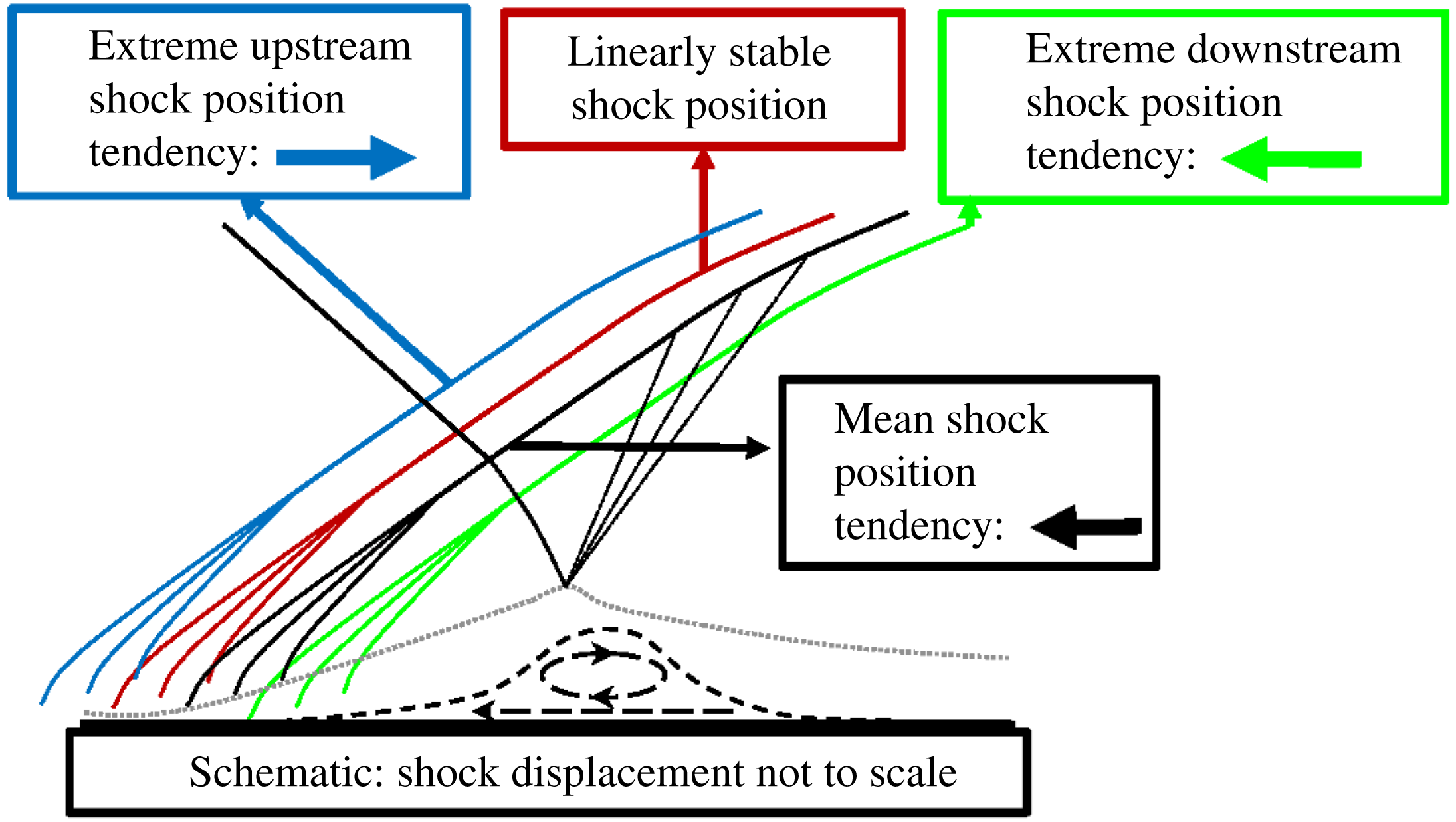
Band-pass filtered mid-frequency separation bubble oscillation:
 $0.06<St_{L}<0.2$
,
 $1.1~\text{kHz}<f<3.6~\text{kHz}$
. (a,c,e,g,i,k) Streamwise velocity base flow with time mean added and arrows indicating base-flow motion. (b,d,f,h,j,l) Streamwise velocity perturbation with arrows indicating time-local linear tendency along the wall and along the separated shear layer. (a)
 $u$
phase 0: bubble downstream
 $(0.7,0.02)$
moving upstream. (b)
 $u^{P}$
phase
 $0$
: bubble downstream
 $(0.7,0.02)$
moving upstream. (c)
 $u$
phase
 $\unicode[STIX]{x03C0}/3$
: bubble midstream
 $(0.5,0.02)$
moving upstream. (e)
 $u^{P}$
phase
 $\unicode[STIX]{x03C0}/3$
: bubble midstream
 $(0.5,0.02)$
moving upstream. (e)
 $u$
phase
 $2\unicode[STIX]{x03C0}/3$
: bubble upstream
 $(0.2,0.02)$
; fluid sheds. (f)
 $u^{P}$
phase
 $2\unicode[STIX]{x03C0}/3$
: bubble upstream
 $(0.2,0.02)$
; fluid sheds. (g)
 $u$
phase
 $\unicode[STIX]{x03C0}$
: bubble moves quickly downstream with shed fluid
 $(0.7,0.02)$
. (h)
 $u^{P}$
phase
 $\unicode[STIX]{x03C0}$
: bubble moves quickly downstream with shed fluid
 $(0.7,0.02)$
. (i)
 $u$
phase
 $4\unicode[STIX]{x03C0}/3$
: bubble
 $(0.9,0.02)$
and shed fluid move downstream. (j)
 $u^{P}$
phase
 $4\unicode[STIX]{x03C0}/3$
: bubble
 $(0.9,0.02)$
and shed fluid move downstream. (k)
 $u$
phase
 $5\unicode[STIX]{x03C0}/3$
: bubble downstream
 $(1.0,0.02)$
; fluid accelerated out of interaction. (l)
 $u^{P}$
phase
 $5\unicode[STIX]{x03C0}/3$
: bubble downstream
 $(1.0,0.02)$
; fluid accelerated out of interaction.

This analysis also suggests that the STBLI permits a time-mean linearly stable configuration, in which the reflected shock is slightly upstream from the time-mean location. At the extremes of the low-frequency cycle (phases
 $\unicode[STIX]{x03C0}/2$
and
 $3\unicode[STIX]{x03C0}/2$
), the bubble and shock motion are consistent with a linear tendency for restoration to a more moderate configuration; previously it was demonstrated that the time-mean base flow is linearly unstable, with a time-mean linear tendency for upstream reflected shock motion, similar to the linearly unstable non-oscillatory mode found in the IVP calculations of Touber & Sandham (Reference Touber and Sandham2009) and the IVP/EVP calculations of Pirozzoli et al. (Reference Pirozzoli, Larsson, Nichols, Bernardini, Morgan and Lele2010) and Nichols et al. (Reference Nichols, Larsson, Bernardini and Pirozzoli2017). Hence, the linearly stable configuration would consist of a separation bubble slightly larger than the time-mean size and a reflected shock slightly upstream from the time-mean location, as indicated in figure 15. Low-frequency unsteadiness could then be described in terms of nonlinear mechanisms forcing the reflected shock, which at extreme displacements experiences a linear tendency for restoration to more moderate displacements, as is the premise of the ODE model proposed by Plotkin (Reference Plotkin1975) and derived by Touber & Sandham (Reference Touber and Sandham2011). However, we find that the ‘time-mean linearly stable shock position’ and the ‘time-mean shock position’ do not coincide, contrary to the assumption of this ODE model, a correction for which could lead to an improved model. We suggest implementing such a correction in the form of a damped and driven harmonic oscillator model, as opposed to the Langevin model that is currently employed; necessarily, to reproduce the shock motion asymmetry with such a model, the stochastic forcing that drives the oscillator should have a functional dependence on the position and velocity of the shock, reflecting contributions from internal mechanisms; e.g. the downstream forcing, resulting from bubble mass depletion, must diminish as the bubble contracts. It follows that, in addition to common techniques which reduce the size of the separation, concepts for control that reduce the discrepancy between the ‘time-mean’ and ‘time-mean linearly stable’ shock positions may prove effective at muting low-frequency unsteadiness.
Oscillation of separation bubble
 $(St_{L}\sim 0.1)$
. Figure 16 shows snapshots of the band-pass filtered
 $(0.06<St_{L}<0.2)$
flow field highlighting oscillation of the separation bubble at frequency
 $St_{L}\sim 0.1$
. In this band, six phases are employed to describe the cycle.
-
$\mathit{Phase}=0:$
-
The bubble (white oval) is downstream (position
$(0.7,0.02)$
) moving upstream. The separated shear layer linearly tends to retard upstream motion (indicated by positive
$u^{P}$
), but along the wall (position
$(0.5,0.02)$
), there is a linear tendency for upstream acceleration of bubble motion (indicated by negative
$u^{P}$
upstream of the current bubble location). -
$\mathit{Phase}=\unicode[STIX]{x03C0}/3:$
-
The bubble is midstream (position
$(0.5,0.02)$
) moving upstream. The shear layer linearly tends to retard upstream motion, but along the wall (position
$(0.5,0.02)$
), there is a linear tendency for acceleration of upstream bubble motion (more extreme than during phase 0). -
$\mathit{Phase}=2\unicode[STIX]{x03C0}/3:$
-
The bubble is upstream (position
$(0.2,0.02)$
), and accelerated by the linear tendency along the wall (position
$(0.2,0.02)$
), but decelerated by the linear tendency away from the wall (position
$(0.2,0.1)$
). The bubble splits: low velocity fluid (pink oval) moves away from wall and is shed downstream, accelerated by the shear layer linear tendency (position
$(0.2,0.1)$
). The shed fluid continues moving downstream. -
$\mathit{Phase}=\unicode[STIX]{x03C0}:$
-
The bubble moves relatively quickly downstream with the shed fluid (position
$(0.7,0.02)$
). This motion is retarded by the shear layer linear tendency. -
$\mathit{Phase}=4\unicode[STIX]{x03C0}/3:$
-
The bubble (position
$(0.9,0.02)$
) and shed fluid continue to move downstream. This downstream motion continues to be retarded by the shear layer linear tendency. -
$\mathit{Phase}=5\unicode[STIX]{x03C0}/3:$
-
The bubble reaches its farthest downstream extent (position
$(1.0,0.02)$
). The bubble and shed fluid are now accelerated downstream, out of interaction region, in accordance with the observed linear tendency. Separation size achieves a minimum. A new near-wall kernel with linear tendency promoting bubble growth and upstream motion appears (position
$(0.4,0.02)$
).


This cycle demonstrates the oscillatory dynamics of the separation bubble at
 $St_{L}\sim 0.1$
. At phase 0, a small negative
 $u^{P}$
kernel appears near the midpoint of the interaction region. The bubble emerges near this position and has a linear tendency to be driven upstream, along the wall, in the initial phases
 $0{-}\unicode[STIX]{x03C0}$
, as demonstrated by the local region of negative
 $u^{P}$
upstream of the current bubble position. During this upstream bubble motion, the linear tendency of the shear layer opposes upstream motion, except in the near-wall, near-bubble region, as demonstrated by a positive region of
 $u^{P}$
. After traversing upstream to near the time-mean separation point, the bubble splits, and some low velocity fluid moves away from the wall entering the off-wall region of faster moving flow (phase
 $2\unicode[STIX]{x03C0}/3$
). The bubble then quickly moves downstream accompanying the shed fluid (phases
 $\unicode[STIX]{x03C0}{-}4\unicode[STIX]{x03C0}/3$
). The shear layer linearly tends to oppose this downstream motion, as indicated by a broad region of negative
 $u^{P}$
. Finally, after traversing downstream to near the time-mean reattachment point, the shed fluid now linearly tends to be accelerated out of the interaction region (indicated by a region of positive
 $u^{P}$
), and the bubble contracts. A new kernel of negative
 $u^{P}$
appears near the interaction region midpoint, and the cycle repeats.
This behaviour is qualitatively similar to several weakly damped oscillatory modes described by Pirozzoli et al. (Reference Pirozzoli, Larsson, Nichols, Bernardini, Morgan and Lele2010) and Nichols et al. (Reference Nichols, Larsson, Bernardini and Pirozzoli2017) in their BiGlobal stability analyses of time-mean STBLI flow fields. Specifically, Nichols et al. (Reference Nichols, Larsson, Bernardini and Pirozzoli2017) describes several weakly damped oscillatory modes
 $(0.06<St_{L}<0.13)$
for a Mach 2.28 STBLI, with an impinging shock generated by a
 $10.7^{\circ }$
far-field wedge. These modes depict periodic oscillations of the separation bubble and reflected shock, similar to our observations of the band-pass filtered
 $(St_{L}\sim 0.1)$
flow fields. The ‘type II’ modes of Nichols et al. (Reference Nichols, Larsson, Bernardini and Pirozzoli2017), in which the ‘reflected shock plays a more passive role’, are particularly similar to the phases of the separation bubble described in figure 16. Additionally,
 $(St_{L}\sim 0.1)$
content is found in the reflected shock signal (figure 10
d), consistent with the ‘type I’ modes, of the BiGlobal analysis, which primarily depict periodic reflected shock motion. However, we suggest a new interpretation of these observations, in conjunction with our recent observations of the dynamic linear response of the time-resolved STBLI: associating the zero-frequency (non-oscillatory) unstable mode with low-frequency
 $(St_{L}\sim 0.03)$
unsteadiness, as discussed in the context of § 5.3.3 and figure 14, and associating the weakly damped oscillatory modes with low–mid-frequency
 $(St_{L}\sim 0.1)$
unsteadiness, as discussed in the context of figure 16. Nonetheless, qualitative agreement between the observed oscillatory behaviour in the LES and BiGlobal stability analyses confirm this mechanism to be an important aspect of low–mid-frequency
 $(St_{L}\sim 0.1)$
STBLI dynamics.
The band-isolated dynamics of the base flow and perturbations are consistent with the action of a mass-depletion mechanism, such as in the conceptual model of Piponniau et al. (Reference Piponniau, Dussauge, Debieve and Dupont2009); the competition of the accompanying nonlinear downstream forcing and upstream linear tendency are necessary to describe the low-frequency dynamics. However, like Morgan et al. (Reference Morgan, Duraisamy, Nguyen, Kawai and Lele2013) we find that the ‘turbulent separation bubble’ (§ 5.3.5) responds more significantly at higher frequencies
 $(St_{L}\sim 0.1)$
than predicted by the model
 $(St_{L}\sim 0.03)$
. Higher-frequency
 $(St_{L}\sim 0.1)$
content is also prominent in the dynamics of subsonic separation unsteadiness (Kiya & Sasaki Reference Kiya and Sasaki1985), and it is not entirely clear that the difference in mixing layer spreading rate, between the low- and high-speed separated flows, fully accounts for the lower frequency
 $(St_{L}\sim 0.03)$
content in the STBLI, without additional considerations of shock-induced effects. Indeed, Agostini, Larchevêque & Dupont (Reference Agostini, Larchevêque and Dupont2015) discuss the significance of the recirculation bubble, with effects unique to this STBLI configuration, in governing both low- and mid-frequency shock dynamics for moderately to massively separated interactions, drawing comparison with aspects of incompressible separated flows.
Furthermore, the prominence of this frequency band in our reverse flow and separation bubble spectra suggests that the accompanying dynamics (figure 16) may be the dominant mechanism for mass transport from the recirculation region to the boundary layer. However, this does not eliminate the possibility for entrainment associated with Kelvin–Helmholtz
 $(St_{L}\sim 0.5)$
shedding to contribute to mass transport from the recirculation region; ultimately, all of these processes are nonlinearly coupled. Notably, this oscillatory mechanism may also be responsible for the ‘low-frequency’ unsteadiness observed by Kiya & Sasaki (Reference Kiya and Sasaki1985). As discussed previously, a potential mechanism for low-frequency
 $(St_{L}\sim 0.03)$
unsteadiness in the STBLI relies on interplay between the linear tendency of the STBLI base flow and nonlinear forcing associated with this oscillatory
 $(St_{L}\sim 0.1)$
mass-depletion mechanism. In the case of Kiya & Sasaki (Reference Kiya and Sasaki1985), there is no shock and thus no interplay to produce unsteadiness at
 $St_{L}\sim 0.03$
, in which case oscillatory bubble mass changes near the frequency
 $St_{L}\sim 0.1$
are the lowest-frequency unsteady features present in that flow. That is, the linear component (figure 14) of the mechanism proposed to describe STBLI unsteadiness at
 $St_{L}\sim 0.03$
only pertains to flows with a similar time-mean linear tendency to the STBLI, and may not pertain to incompressible separated flows, since the separation is not shock induced. For these cases, the linear oscillatory mechanism (figure 16) proposed to describe STBLI unsteadiness at
 $St_{L}\sim 0.1$
may be the primary mechanism of ‘low-frequency’ unsteadiness.
Band-pass filtered mid-frequency Kelvin–Helmholtz shedding:
 $0.2<St_{L}<0.7$
,
 $3.6~\text{kHz}<f<12.7~\text{kHz}$
. (a,c,e,g,i) Streamwise velocity base flow with time mean added and arrows indicating base-flow motion. (b,d,f,h,j) Streamwise velocity perturbation with arrows indicating time-local linear tendency. (a)
 $u$
phase
 $0$
: pink wave crest peak. (b)
 $u^{P}$
phase
 $0$
: pink wave crest peak. (c)
 $u$
phase
 $\unicode[STIX]{x03C0}/2$
: white grows, pink recedes. (d)
 $u^{P}$
phase
 $\unicode[STIX]{x03C0}/2$
: white grows, pink recedes. (e)
 $u$
phase
 $\unicode[STIX]{x03C0}$
: white grows, pink recedes. (f)
 $u^{P}$
phase
 $\unicode[STIX]{x03C0}$
: white grows, pink recedes. (g)
 $u$
phase
 $3\unicode[STIX]{x03C0}/2$
: white grows, pink recedes. (h)
 $u^{P}$
phase
 $3\unicode[STIX]{x03C0}/2$
: white grows, pink recedes. (i)
 $u$
phase
 $0$
: white wave crest peak. (j)
 $u^{P}$
phase
 $0$
: white wave crest peak.

Kelvin–Helmholtz (K–H) shedding
 $(St_{L}\sim 0.5)$
. Figure 17 shows snapshots from the band-pass filtered
 $(0.2<St_{L}<0.7)$
flow field highlighting K–H phenomena at frequency
 $St_{L}\sim 0.5$
. The base flow clearly demonstrates wave-like motion through the recirculation region, which corresponds to flapping of the reflected shock foot. K–H waves in this frequency band contribute to the origin of shed structures, leading to dominant mid-frequency
 $(St_{L}\sim 0.5)$
content in the post-interaction wall pressure spectra of figure 11(a). We note, however, as shown in the reverse flow and separation bubble spectra of figure 10(d), that the mass of fluid in the recirculation region does not respond significantly at this frequency, and instead simply rides the waves. This suggests that while K–H
 $(St_{L}\sim 0.5)$
waves originate in the separation region and account for the increase in convective content around
 $St_{L}\sim 0.5$
downstream of the interaction, it is insufficient to describe the mid-frequency separation bubble dynamics without noting both the oscillatory behaviour in the
 $St_{L}\sim 0.1$
band, as well as wave-like behaviour in the
 $St_{L}\sim 0.5$
band.
Since this band approaches higher frequencies
 $(St_{L}\sim 1)$
associated with convecting fine-scale turbulence, we observe more significant contamination from turbulence and flow history effects in the corresponding band-pass filtered perturbation field than in previous lower-frequency bands. Still, periodic changes in the perturbation field character near the time-mean separation point and along the separated shear layer coincide with the genesis frequency and convection of K–H waves, suggesting that these may also be driven by a periodic linear mechanism acting throughout the interaction; the separation bubbles are approximately driven along the major gradients of high to low (red to blue) streamwise velocity perturbation, consistent with the observed linear tendency. The clarity of the band-pass filtered perturbation field in this higher-frequency band could be improved through a conditional analysis, but is not considered in the current work.
This sequential low-pass filtering analysis thus aids in understanding the dynamic relation between the base-flow and linearly constrained perturbation fields in different frequency bands. In each frequency band, and at specific phases, it allows for the identification of whether the STBLI is responding consistently with the time-local linear mechanisms identified in the evolving flow, or responding contrary to the identified linear mechanisms, suggesting the increased importance of nonlinear mechanisms. We anticipate that these linear mechanisms are an essential source of unsteadiness in all similar STBLIs, including those that are influenced by low-frequency coherent fluctuations of the incoming flow, though such coherent fluctuations are not observed in the present study; the relative significance of internal to external mechanisms as sources of unsteadiness remain flow-specific questions. Although this analysis does not demonstrate a statistically robust measure of the dynamical behaviour in each frequency band, it does identify clear trends associated with each frequency band that are qualitatively similar throughout many realizations. As such, it successfully illustrates several key unsteady broadband features present in the STBLI and aids in identifying potential linear mechanisms which may sustain these features in the unsteady turbulent environment.
6 Conclusions
A Mach 2.3 shock/turbulent-boundary-layer interaction is studied through small amplitude (linear) forcing of the unsteady separated flow. The response to this forcing is obtained by solving a constrained linearization about the time-evolving turbulent flow. For this purpose, a synchronized pair of large-eddy simulations is employed, in which the two simulations are advanced synchronously in time, with the second simulation constrained linearly to the first. The two solutions are processed to yield the evolution of linear perturbations of the fully turbulent STBLI. Ensemble statistics of the linear perturbations constitute the dynamic linear response of the flow, analysis of which allows for the inference of both the time-mean as well as the time-local linear tendencies of the unsteady turbulent flow. In limiting cases, these tendencies are analogous to and qualitatively consistent with traditional stability analyses applied to the steady time-mean base flow.
The dynamic linear response demonstrates that the STBLI fosters a global absolute linear instability corresponding to a linear tendency for upstream shock motion and enlargement of the separation bubble. The absolute instability is maintained through constructive feedback of perturbations through the recirculation; it is self-sustaining and insensitive to external forcing. In contrast, this phenomenon is not observed in similarly perturbed turbulent boundary layers, in which linearly constrained perturbation growth is convective in nature and sustained only through continuous external forcing. The self-sustaining perturbation field of the STBLI is similar in character to the perturbation field forced at a location inside the time-mean recirculation region, indicating that perturbations originating in the recirculation region have a more significant influence on STBLI dynamics than those originating upstream. The perturbation field remains anchored to the interaction region and exhibits a time-mean linear tendency for upstream motion of the reflected shock. This non-zero time-mean linear tendency quantifies the nature of the global absolute linear instability, and its bias for upstream motion is inherently coupled to observed asymmetry in the low-frequency shock motion cycle, in which upstream shock motion occurs rapidly followed by slower downstream motion.
Significant dynamic features of the STBLI are identified and delineated by key frequency bands:
 $St_{L}\sim 0.5$
corresponding to high–mid-frequency Kelvin–Helmholtz shedding along the separated shear layer,
 $St_{L}\sim 0.1$
corresponding to low–mid-frequency oscillations of the separation bubble, and
 $St_{L}\sim 0.03$
corresponding to low-frequency large-scale bubble breathing and shock motion. Informed by observation of these frequencies in the STBLI, a band-pass filtering decomposition is applied to the STBLI base-flow and perturbation fields to isolate these broadband features and identify how the time-local linear tendencies of the STBLI contribute to mid-frequency and low-frequency dynamics.
The low-frequency
 $(St_{L}\sim 0.03)$
breathing of the separation bubble and corresponding shock motion can be explained in the context of competing linear and nonlinear mechanisms; linear mechanisms are identified from the dynamic linear response, and nonlinear mechanisms include mass depletion from the recirculation region through shedding during bubble contraction. This proposed explanation also accounts for the observed asymmetry in the low-frequency cycle. Furthermore, this analysis confirms the presence of linear restoring tendencies in the STBLI; when the reflected shock is located at an extreme upstream or downstream displacement from its time-mean position, a linear tendency for restoration to a more moderate position is observed. However, this moderate position (a linearly stable position in the time-mean sense) does not correspond with the time-mean shock position, but rather is located upstream from the time-mean shock position. This observation that the ‘time-mean linearly stable position’ and the ‘time-mean position’ do not coincide supports the assertion that the low-frequency unsteadiness is an intrinsic property of the system, which could potentially be mitigated through control by altering the interaction in a way such that the two positions are more closely coincident.
The separation bubble is found to oscillate at mid-frequency
 $(St_{L}\sim 0.1)$
in accordance with the linear tendency of the STBLI, and the mass budget of the recirculation region is also affected prominently at this frequency, suggesting that mass depletion of the recirculation region may be due to shedding observed during this oscillatory cycle. The separation bubble exhibits wave-like behaviour in the
 $St_{L}\sim 0.5$
band, consistent with Kelvin–Helmholtz shedding, which is identified downstream of the interaction region in wall pressure spectra. However, the mass budget of the reverse flow region does not indicate significant dynamics at this frequency, and rather it is observed that the bubble simply rides the waves. While it is more challenging to draw conclusions at this higher frequency regarding how the Kelvin–Helmholtz shedding is influenced by linear mechanisms due to a greater degree of contamination from high-frequency turbulence, the results are not inconsistent with the possibility that this shedding is also sustained by linear mechanisms evident throughout the interaction.
Acknowledgements
The authors acknowledge several insightful conversations with Dr P. Schmid, Dr L. Agostini and Dr S. Unnikrishnan, and appreciate the sponsorship of the US Air Force Office of Scientific Research (Monitor: Dr I. Leyva, contract FA955014-1-0167). M.C.A. is supported through the US National Defense Science and Engineering Graduate Fellowship (NDSEG) Program. The simulations described were performed with grants of computer time from the US Department of Defense HPCMP shared resources at AFRL, NAVO and ERDC. Some figures have been made with complimentary licenses of FieldView obtained from Intelligent Light under the University Partners Program.


 Open access

