

1. Introduction
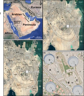
The Dammam Dome, which is located in the eastern part of the Arabian Peninsula (Fig. 1a) constitutes the first and main hydrocarbon structural trap found in the Eastern Province of Saudi Arabia. It covers c. 500 km2 and encompasses the cities of Al Khobar, Al Dhahran and part of Ad Dammam (Hariri, Reference Hariri2014).
Satellite Google Earth images of (a) the Arabian Peninsula and the Zagros fold belt with the location of the Dammam Dome in the Eastern Province of Saudi Arabia; (b) the topography of the Dammam Dome shown by height contours; (c) the simplified geological map with the exposed map units of the Dammam Dome; and (d) the studied exposures A, B, C and D on the KFUPM campus. (c) and (d) are based on and modified after Weijermars (Reference Weijermars1999). Abbreviations: MZT: Main Zagros Thrust; ZFB: Zagros Fold Belt; KFUPM: King Fahd University of Petroleum and Minerals; E-LR: Eocene Lower Rus Formation; E-UR: Eocene Upper Rus Formation; E-Dm: Eocene Dammam Formation; Ng-Th: Neogene Hadrukh Formation; Q: Quaternary undivided. In (a) the maximum compressive stresses are shown with opposite-directed arrows (black: pre-Late Miocene; white thin: post-Late Miocene – Pliocene, based on Lacombe et al. (Reference Lacombe, Mouthereau, Kargar and Meyer2006); white thick: present-day based on Ameen et al. (Reference Ameen, Buhidma and Rahim2010) and Ameen (Reference Ameen2014)). In (d) equal-area, lower-hemisphere projections show the VCT structures as white balls, and the host planes with both great circles and poles (solid black circles); 4, 7, 14, 15 are the label numbers of the KFUPM buildings.

Previous work on the Dammam Dome includes a detailed surface map of the core region of the dome, drawing on proprietary Saudi Aramco data, aerial photographs and field observations (Tleel, Reference Tleel1973). Weijermars (Reference Weijermars1999) performed a geological compilation of the Dammam Peninsula on a modern road map to facilitate academic and professional field studies and engineering operations. More recently, fracture analyses of the Dammam Dome has been carried out and presented by Hariri & Abdullatif (Reference Hariri and Abdullatif2005), Al-Fahmi (Reference Al-Fahmi2012), Al-Fahmi et al. (Reference Al-Fahmi, Michele and Cole2014) and Hariri (Reference Hariri2014). Hariri (Reference Hariri2014) conducted an intensive fracture study and analysis in five outcrops in order to define the driving stresses and mechanisms forming the Dammam Dome, more specifically, on the campus of King Fahd University of Petroleum & Minerals (KFUPM), which is located at the apex of the dome.
These studies focus on brittle deformation structures (e.g. Al-Fahmi Reference Al-Fahmi2012; Al-Fahmi et al. Reference Al-Fahmi, Michele and Cole2014; Hariri, Reference Hariri2014) but do not provide any connection between deformation of the Dammam Dome region and intraplate stresses associated with large-scale tectonic processes along the neighbouring active plate boundaries. These large-scale tectonic processes operate mainly along the Zagros orogen, the largest mountain belt and the most active collisional orogen associated with Arabia/Eurasia convergence (Dewey & Grantz, Reference Dewey and Grantz1973; Dercourt et al. Reference Dercourt, Zonenshain, Ricou, Kazmin, Le Pichon, Knipper, Grandjacquet, Sbortshikov, Geyssant, Lepvrier, Pechersky, Boulin, Sibuet, Savostin, Sorokhtin, Westphal, Bazhenov, Lauer and Biju-Duval1986; Stampfli & Borel, Reference Stampfli and Borel2002) to the east. Moreover, there is other tectonism to the west associated with opening of the Red Sea (Bosworth et al. Reference Bosworth, Huchon and McClay2005) to the west. However, the Dammam Dome region, as part of the Arabian platform, is in the interior of the Arabian plate, and thus far away from plate boundaries. As a result, any relation between the Dammam Dome and the stresses and processes along these boundaries is difficult to determine.
Sources of intraplate stresses can be divided into three broad classes: (1) stresses related to the driving mechanism of plate tectonics, (2) stresses related to the cooling of the lithosphere and (3) stresses remaining in the lithosphere from geological processes that are no longer active (Sykes & Sbar, Reference Sykes and Sbar1974). Studies have demonstrated a causal relationship between the processes at plate boundaries and the deformation in the plate interiors (e.g. Johnson & Bally, Reference Johnson and Bally1986), while the intraplate deformation results from the transmission of intraplate stress fields away from plate boundaries into continental forelands (Van der Pluijm et al. Reference Van der Pluijm, Craddock, Graham and Harris1997; Ziegler et al. Reference Ziegler, Van Wees and Cloetingh1998; Tesauro et al. Reference Tesauro, Hollenstein, Egli, Geiger and Kahle2005; Schellart & Moresi, Reference Schellart and Moresi2013). In addition, intraplate stresses and vertical motions of several sedimentary basins in the interior of plates (Cloetingh, Reference Cloetingh1988; Cloetingh & Burov, Reference Cloetingh and Burov2011) could result from lithospheric folding caused by the stresses along plate boundaries. However, most studies have concentrated on intraplate deformation of the overriding or upper plate in a plate convergence system, possibly because the tectono-magmatic events are much better constrained. On the other hand, intraplate deformation in the subducting or lower plate has not attracted as much interest because, as a rule, the deformation is very low, making it difficult to interrelate the scarce exposed brittle structures to deformation along the plate boundaries, which is the case in this study. Moreover, the analysis of joints and fractures studied in the region of the Dammam Dome does not provide any strong evidence for interrelating intraplate stresses with stresses originating in the plate boundaries (Al-Fahmi Reference Al-Fahmi2012; Al-Fahmi et al. Reference Al-Fahmi, Michele and Cole2014; Hariri, Reference Hariri2014). In contrast, published in situ stress measurements show that intraplate stresses in the Eastern Province of the Arabian platform are dominated by the Zagros plate tectonics (Ameen et al. Reference Ameen, Buhidma and Rahim2010; Ameen, Reference Ameen2014).
The present study documents ‘odd’ structures, which are exposed in outcrops on the KFUPM campus and described here, in detail. Despite these structures being observable, they have been neglected, possibly due to misinterpretation or peculiarity. Nonetheless, these are soft-sediment structures formed during the final stages of diagenesis before lithification was complete due to transport slip along a soft-sediment (or hydroplastic) detachment, which is referred as the Rus detachment.
These soft-sediment structures are significant because they allow the dating of deformation, which in the shallower levels of the crust is not possible by geochronological methods as temperatures are too low for recrystallization (Ortner, Reference Ortner2007). The aim of this paper is to demonstrate that, in contrast to brittle structures, soft-sediment structures provide interesting clues about intraplate stresses and their interrelationship with plate boundary stresses originating from collision processes along the Zagros orogen.
2. Geological setting
Topographic maps of the Dammam Peninsula (Fig. 1b) indicate a large NNW–SSE (∼330°) oval hill (∼14 km × 9 km) of elevation no higher than 150 m (Weijermars, Reference Weijermars1999). This geomorphological structure is the Dammam Dome, a large oval-shaped structural dome as shown in the geological map of Weijermars (Reference Weijermars1999) compiled from existing source maps (Steineke et al. Reference Steineke, Bramkamp and Sander1958; Tleel, Reference Tleel1973; Roger & Giot, Reference Roger and Giot1985) (Fig. 1c). The Rus Formation occupies the core of the Dammam Dome, on which both the Saudi Aramco and KFUPM campuses have been established.
The Dammam Dome, because of its strong negative gravity anomaly and oval shape (Powers et al. Reference Powers, Ramirez, Redmond and Elberg1966), and the nearby Awali Dome below Bahrain Island (c. 50 km south) are considered to be cored by a salt layer, lying at depths of c. 10–12 km between the Precambrian basement and the overlying Phanerozoic sequences of the Arabian Platform (see Weijermars, Reference Weijermars1999: fig. 7). This salt layer, the Hormuz Salt (Beydoun, Reference Beydoun1991; Bahroudi & Koyi, Reference Bahroudi and Koyi2003; Stern & Johnson, Reference Stern and Johnson2010; Stewart, Reference Stewart2018), is considered to be the detachment layer over which the accretionary wedge of the Zagros orogen has developed, forming the Zagros Fold Belt (ZFB) (Colman-Sadd, Reference Colman-Sadd1978; Edgell, Reference Edgell1996; Talbot & Alavi Reference Talbot and Alavi1996; Bahroudi & Koyi, Reference Bahroudi and Koyi2003; Bigi et al. Reference Bigi, Carminati, Aldega, Trippetta and Kavoosi2018). However, structural models into which the Hormuz evaporitic layer is the main basal décollement have shown that this structure alone is unlikely to maintain the regional topography (Mouthereau et al. Reference Mouthereau, Lacombe and Meyer2006).
The Dammam Dome plunges to the southeast at c. 1°12′, and to the northwest slightly less than 1°, and its flanks are very gentle (average dips on the northeast and southwest flanks are 1°30′ and 1°10′, respectively) (Tleel, Reference Tleel1973). As a result, Weijermars (Reference Weijermars1999) posed the question whether the formation of the Dammam Dome is directly related to compressional tectonic stresses, even though the average Cenozoic growth rate inferred from stratigraphic relationships within the Dammam Dome suggests uplift rates of 7 to 7.5 m/My for most of the Cenozoic.
The exposed sedimentary rocks of the Dammam Dome have been grouped into the following formations from bottom to top (Powers et al. Reference Powers, Ramirez, Redmond and Elberg1966): (a) Rus Formation, (b) Dammam Formation, (c) Hadrukh Formation and (d) Dam Formation. The first two formations are dated as Eocene, whereas the latter two are dated as Lower Miocene due to a major unconformity that is generally referred to as the Pre-Neogene Unconformity (PNU) (Tleel, Reference Tleel1973). The PNU is associated with the lack of deposition during the Oligocene throughout the entire Arabian Platform. As the last two aforementioned formations are outside the scope of this study, detailed descriptions of them were purposely left out as information about them can be obtained in previously published papers.
The Rus Formation is exposed in the central part of the dome (Fig. 1c) and overlies the Palaeocene to Early Eocene Umm er Radhuma (UER) Formation (SB Henry and CW Brown in 1935 (unpublished Aramco report)). The Rus Formation was dated as Early Eocene (Ypresian, 57.8 to 52.0 Ma; Palmer, Reference Palmer1983) and is underlain and overlain by rocks of Early Eocene age, although no diagnostic fossils have been identified (Powers et al. Reference Powers, Ramirez, Redmond and Elberg1966). Tleel (Reference Tleel1973) divided the Rus Formation into three informal zones:
-
(a) the Lower Rus, which consists of 21 m of alternations of marls and thin grey-to-buff dolomitic limestone beds, abundant slumps and quartz geodes (Zone of Quartz Geods; Tleel, Reference Tleel1973),
-
(b) the Middle Rus, which is well fractured and consists of 10 m of thick grey-buff calcarenite, abundant mud balls, vuggy weathering and calcite geodes (Zone of Calcite Geods; Tleel, Reference Tleel1973),
-
(c) the Upper Rus (Chalky Zone of Tleel, Reference Tleel1973), which consists of 25 m of yellow-grey, microcrystalline to cryptocrystalline, partly dolomitic, limestone and white chalky aphanitic limestone, few marl horizons, and clay layers on top. Three thin bands of continental, yellow-orange, gypsiferous shale, locally purple weathered, are valuable markers in the upper Rus section (Roger & Giot, Reference Roger and Giot1985). Chert pods or nodules of pebble to boulder size are the most striking feature in the white ‘chalky’ limestone at the top of the Rus Formation (Weijermars, Reference Weijermars1999).
However, Tleel (Reference Tleel1973) subdivided the three informal zones of the Rus Formation into two map units selected strictly for mapping convenience: (1) the Lower Rus (including the first two informal zones) and (2) the Upper Rus (including the last informal zone), and this geological mapping was followed by Weijermars (Reference Weijermars1999) in his compiled geological map and is also used herein (Fig. 1c). In general, the Rus Formation was deposited in a restricted lagoonal to supratidal sabkha setting. As a general rule, the middle Rus is thicker on the flanks of structures than it is on the crests (Powers et al. Reference Powers, Ramirez, Redmond and Elberg1966). The Dammam Formation, coined by Bramkamp (Saudi Aramco report of 1941; see Powers et al. Reference Powers, Ramirez, Redmond and Elberg1966), rests conformably on top of the Rus Formation and is subdivided into five members. From bottom to top these are: (1) the Midra Shale (up to 3 m in outcrop, but as much as 8 m in subsurface), (2) Saila Shale (up to 4 m in outcrop, but as much as 12 m in drill holes), (3) Alveolina Limestone (0.9 to 2 m in outcrop, but up to 12 m in subsurface), (4) Khobar (6.8 to 11 m) and (5) Alat (15 m) members. The two lower members are of Ypresian age (57.8 to 52.0 Ma; Palmer, Reference Palmer1983), but the Alveolina Limestone, Khobar and Alat members are of Lutetian age (52.0 to 43.8 Ma; Palmer, Reference Palmer1983).
Previous authors consider both possible undercutting in the Eocene stratigraphy and the structural growth of the dome to be a positive feature that explains the observations of omission or thinning-out of some stratigraphic units and slumping, the latter being a common feature on the Dammam Dome (Powers et al. Reference Powers, Ramirez, Redmond and Elberg1966; Tleel, Reference Tleel1973). For example, we consider the thinning-out of both the Midra Shale and Saila Shale units toward the crest of the dome and the omission of Alat exposures within the rimrock. However, structural growth is limited (Tleel, Reference Tleel1973) due to minor angular discordance between the Eocene and the overlying Miocene strata. In addition, the middle Eocene (post-Alat) was a period of broad emergence across the Arabian platform, which explains why most of the Arabian platform has positive structural features, as in the Dammam Dome. Slumping has also been recognized in the Lower Rus Formation (Tleel, Reference Tleel1973; Weijermars, Reference Weijermars1999). However, some structures which were interpreted as slumping may instead be faulting (Tleel, Reference Tleel1973). The Dammam Formation represents a transgressive sequence where the sabkha and subtidal to continental lagoon were progressively transformed into an open-marine environment (Weijermars, Reference Weijermars1999).
The fracture pattern in the Dammam Dome has attracted interest from the geological community since the proposal of Stearns’s model (Stearns, Reference Stearns and Rieker1968) and its sequential improvements (Stearns & Friedman, Reference Stearns and Friedman1972; Price & Cosgrove, Reference Price and Cosgrove1990), which relates specific fracture patterns to the fold geometry. Based on the outcrops located on the KFUPM campus, Weijermars (Reference Weijermars1999) reported that jointing is irregular and rare in the Lower Rus unit, due to the presence of incompetent marls. In contrast, regularly spaced joints are characteristic of the Middle Rus formation. Hariri & Abdullatif (Reference Hariri and Abdullatif2005) delineated the lineaments from Landsat images using GIS software, and Al-Fahmi (Reference Al-Fahmi2012), Al Fahmi et al. (Reference Al-Fahmi, Michele and Cole2014) and Hariri (Reference Hariri2014) studied the rock exposures of the Dammam Dome more systematically, to better understand the exposed fractures. The described fracture pattern includes a dominant joint set striking NW–SE parallel to the major axis of the dome, and a younger joint set striking NE–SW such that both sets form an orthogonal fracture pattern (Al-Fahmi, Reference Al-Fahmi2012). Al-Fahmi (Reference Al-Fahmi2012) stated that the NW–SE-striking joints are not compatible with the regional stress regime, but they are related to the fold growth of the strata, position on the fold, and mechanical stratigraphy. In addition, Hariri (Reference Hariri2014) suggested a model for this fracture-dome relationship.
On the other hand, published information from in situ stress measurements performed in the Khuff reservoir from 19 onshore structural traps of the Eastern Province (Ameen et al. Reference Ameen, Buhidma and Rahim2010) and eastern offshore Saudi Arabia (Ameen, Reference Ameen2014) show that the present-day maximum horizontal in situ stresses (
 ${\sigma _{\rm{H}}}$
) trend E–W to ENE–WSW dominated by Zagros tectonics, whereas the minimum horizontal in situ stress (
 ${\sigma _{\rm{h}}}$
) is N–S to NNW–SSE. The high horizontal stress anisotropy (Ameen et al. Reference Ameen, Buhidma and Rahim2010), and the magnitudes of in situ stresses estimated from field data, laboratory tests of cores, and analysis of stress indicators from image logs in vertical wells (Ameen, Reference Ameen2014) invariably indicate that the stress regime is strike-slip (
 ${\sigma _{\rm{H}}}\,$
>
 ${\sigma _{\rm{V}}}$
>
 ${\sigma _{\rm{h}}}$
), whereas the stress regime can be of transitional extensional to strike-slip nature (
 ${\sigma _{\rm{H}}}$
≥
 ${\sigma _{\rm{V}}}\,$
>
 ${\sigma _{\rm{h}}}$
) locally.
In contrast, brittle structures in the region of the Dammam Dome do not indicate any relation with plate boundary processes associated with the Zagros orogen, even when the orogenic processes due to Eurasia/Arabia convergence changed from subduction to collision along the Zagros orogen. The timing of the onset of this continental collision along the Zagros Mountains is generally considered to have initiated at ∼35 Ma as the rifted Arabian lithosphere was underthrusted due to its negative buoyancy beneath the Iranian plate (Mouthereau et al. Reference Mouthereau, Lacombe and Vergés2012). Moreover, the exact time of collision is poorly constrained as having occurred between Late Cretaceous and Pliocene times (e.g. Berberian & King, Reference Berberian and King1981; Alavi, Reference Alavi1994; Agard et al. Reference Agard, Omrani, Jolivet and Mouthereau2005; Sherkati et al. Reference Sherkati, Letouzey and Frizon de Lamotte2006) and remains a matter of debate (Ahmadhadi et al. Reference Ahmadhadi, Lacombe and Daniel2007; Zhang et al. Reference Zhang, Xiao, Majidifard, Zhu, Wan, Ao, Chen, Rezaeian and Esmaeili2017).
Arabia–Eurasia convergence along Zagros is trending N–S to NNE–SSW as shown by recent GPS studies at the Arabian plate scale and corresponds to a velocity of about 22–25 mm/yr in a N010°E direction at a longitude 56° E (McClusky et al. Reference McClusky, Reilinger, Mahmoud, Ben Sari and Tealeb2003; Vernant et al. Reference Vernant, Nilforoushan, Hatzfeld, Abbassi, Vigny, Masson and Chéry2004). A similar N020°–030° compression associated with a reverse-strike-slip faulting and a low ratio between differential stresses has been defined by the inversion of small and moderate earthquakes in the Western Fars (Iran) that accounts for the combination of strike-slip and thrust-type focal mechanisms through likely σ 2/σ 3 permutations (Lacombe et al. Reference Lacombe, Mouthereau, Kargar and Meyer2006). In addition, their fault-slip analysis reveals two successive late Cenozoic regional compressional trends, the N020° and a relatively older NE–SW. The first case fits well with the present-day stress, whereas the latter is associated with the main folding phase at regional scale, which began to develop as soon as Oligocene – early Miocene times toward the Arabian craton forming the ZFB (Lacombe et al. Reference Lacombe, Mouthereau, Kargar and Meyer2006).
3. Soft-sediment (hydroplastic) deformation
Soft-sediment deformation is commonly recognized in most sediment gravity flow systems since the latter is dominated by a mixture of water and sediment. Furthermore, the field description of syn-sedimentary faults and hydroplastic faulting is generally very limited (e.g. Petit & Laville, Reference Petit and Laville1987). However, direct observations of hydroplastic faults provide one of the most important ways of checking whether subsidence is linked to dip-slip, strike-slip or oblique-slip faults since this involves determining the orientation and directions of relative movement on proven syn-sedimentary fault planes (Petit & Laville, Reference Petit and Laville1987).
The odd structures, described herein for the first time occur at different KFUPM campus sites A, B, C and D in Figure 1d, and they have previously been ignored or misinterpreted. Some of these sites are more than 200 m apart from each other and this large distance dictates that these odd structures occur due to regional rather than local reasons. The exposed rock at these sites is a massive microcrystalline limestone with no bedding, constituting the Middle Rus Formation. The odd structures occur within the first few metres (commonly less than 2 m) above its boundary/interface with the underlying Lower Rus Formation. These odd structures are interpreted herein as hydroplastic kinematic indicators that indicate slip towards NNW (345°) and they are attributed to the soft-sediment detachment activity of the Middle and Lower Rus boundary/interface, referred to herein as the Rus soft-sediment detachment.
3.a. Description of the odd hydroplastic structures
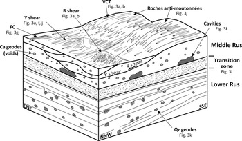
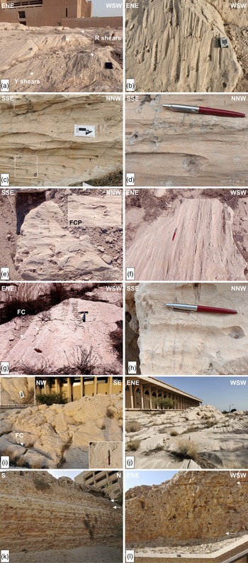
The odd hydroplastic structures occur mostly on the flat upper part of the massive microcrystalline limestone exposures along flat-lying to gently dipping surfaces (Figs 2, 3a). They are vugs ranging in diameter from 1 to 5 cm and on rare occasion up to 10 cm, i.e. fist-sized cavities that commonly exhibit ‘carrot-shape’ or ‘comet-shape’ tails as rock imprints (Figs 2, 3b, c), labelled as ‘Vugs-Carrot/Comet-Trail’ (VCT) structures. These vugs mark the places of geodes or nodules filled with calcite crystal assemblages that have been eroded out due to weathering. The VCT structures are similar to the imprints of crag-and-tail structures described for brittle deformation by Tjia (Reference Tjia2014) or the trailed material (TM) of Doblas (Reference Doblas1998). This interpretation is based on the presence of lined calcite microcrystalline masses within some of these vugs, whereas few calcite geodes have been found in situ (Figs 2, 3c, d). More rarely, another interesting structure has been observed on the exposed surfaces. It is the ‘front cat paw’ (FCP) (Fig. 3e) imprint, so named due to its resemblance to a cat’s paw, as seen from the front.
Three-dimensional sketch block showing the soft-sediment Rus Detachment, i.e. the contact between the Lower and Middle Rus Fm, and the associated structures observed and shown in Figure 3. VCT: vug with carrot- or comet-shape tail structure; FC: flute or channel structure.

Field photographs of (a) the exposures of Y and R shears containing VCT structures (site A); (b) the VCT structures (site A); (c) the VCT structures (site B). Square shows the position of photo (d); (d) detail view of the square shown in (c) showing the remaining calcite geodes forming the VCT structures, and the extension fracture qz-veinlets perpendicular to the VCT structures; (e) FCP structures on Y shears (site A); (f, g) flute or channel (FC) structures on Y shears (site B); (h) VCT structures and extension fractures perpendicular to VCT (site D); (i) flute or channel (FC) structures on Y shears and P shears in the square. Detail of the P shear surface is shown in the two edge inset photos; (j) the morphotectonic feature similar to ‘roches moutonnées’ but of opposite standing to the transport direction (site B); (k) the natural profile of the passage from the underlying Lower Rus to the Middle Rus Formation. Cavities and white arrows indicate the fluid-escape zone at the base of the Middle Rus. Lower Rus consists of marls and marlstones in alternations with abundant geodes (next to hammer); (l) the fluid-escape zone between the underlying marls of the Lower Rus and the overlying massive limestone of the Middle Rus shown by the two arrows. The zone is a cemented mixture of material and cobble- or boulder-size blocks with fractures, voids and cavities.

The observed surfaces containing the VCT structures just above the Rus detachment, which is considered as the principal deformation zone, can be classified as (a) Y slip surfaces (Figs 2, 3a), (b) R shears (Figs 2, 3a) and (c) P shears, considering their orientations. The Y, R and P surfaces can be described as hydroplastic slickensides (terminology according to Petit & Laville, Reference Petit and Laville1987).
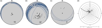
The Y surfaces are metric-scale smooth to polished surfaces containing in places slickenlines (Fig. 3f) that resemble features more akin to stretching lineations, rather than striations, thus indicating the low, if not absence of, friction along the slip direction. They are flat and generally planar dipping with no more than 15° towards the NNW (Fig. 4a). Locally, these surfaces occur with flutes or channels (FC) parallel to the transport direction with lengths up to 1.5 to 2 m and radii up to c. 10 cm. FC arrays are joined with angular-shaped ridges resembling the grooves or cannelures formed by glacier movements but without striations and frictional grooves (Fig. 3g). Nonetheless, the fist-sized VCT structures are not the dominant structures on these surfaces.
Equal-area, lower-hemisphere projections of the (a) Y shears (n = 10), (b) R shears (n = 37) and (c) P shears (n = 3), indicating transport direction towards the NNW, and (d) tangent diagram of the Y and R shears defining a conical surface that plunges towards NNW at c. 20°. In (b) dashed lines show the curvature of the R shears.

The R shears dip from 18° up to 40° towards NNW (Fig. 4b). The dominant feature is the VCT structures, which show constant transport of the hanging wall towards the NNW. In addition, some cm-scale extension fractures occur filled with clastic material orientated perpendicular to the NW-NNW stretching (Fig. 3h).
The P shears are very few, expressed as small surfaces dipping to the S-SSE at angles from 35° to 45° (Fig. 4c) containing a few VCT structures (Fig. 3i) showing a congruous sense of slip, like the Y and R shears.
The Y and R shears form in combination with metric- to decametric-scale long morphotectonic features, named ‘roches anti-moutonnées’ as they have morphologies similar to ‘roches moutonnées’ formed by glacier movement, but these features stand opposite to the transport direction (Fig. 3j). These morphotectonic features are characterized by strain compatibility (Fig. 4b) (i.e. slip that occurred parallel to the intersection of the fault planes, Marrett & Allmendinger, Reference Marrett and Allmendinger1990), and have a conical surface, the apex of which plunges c. 20° towards NNW (350°), as defined by the projection of the R shears onto the Bengtson’s (Reference Bengtson1981) tangent diagram (Fig. 4d).
3.b. Hydroplastic deformation mechanism
A characteristic behaviour common in weak porous and unconsolidated sediments is hydroplastic behaviour, which is situated in the rheologically transitional field between brittle and ductile deformation (Petit & Laville, Reference Petit and Laville1987). Soft-sediment deformation occurs in sediments through mechanisms like independent particulate flow, diffusion mass transfer and cataclasis (Knipe, Reference Knipe1989) because of the interstitial fluid, which is trapped, making the pore pressures relatively high and potentially unstable. The deformation ratio, degree of lithification and fluid pressure are the controlling factors to the soft-sediment deformation, which changes progressively with the increase of sediment burial (Knipe, Reference Knipe1989).
The VCT structures described previously are better explained by independent particulate flow. The latter is an intergranular mode of deformation resulting in ductile flow on an aggregate scale. This mechanism involves the sliding of grains moving past and over each other without any deformation of the particles and is controlled by shearing at grain boundaries or surfaces (Handin et al. Reference Handin, Hager, Friedman and Feather1963; Verrall et al. Reference Verrall, Fields and Ashby1977; Borradaile, Reference Borradaile1981). Moreover, this is the only possible mechanism of straining when frictional grain boundary sliding occurs, though the individual grains do not deform internally (Borradaile, Reference Borradaile1981).
Generally, the fluid pressure in the massive microcrystalline limestone of Middle Rus is lower than the grain weight and is preserved in the sediment since no extensive fluidization has occurred. The only structures that can be considered to have resulted from fluidization, are the vertical beds in the Lower Rus, reported and attributed to slumping processes (Weijermars, Reference Weijermars1999), though they were nowhere to be found. On the other hand, the existence of a ‘transition zone’ at the uppermost part of the Lower Rus (Fig. 2) suggests upward fluid-escape from Lower Rus. This transition zone consists of carbonate rock formed by the assemblage of cobble-to-boulder-size carbonate blocks that appear lithified into a massive impure carbonate matrix with voids (Fig. 3k) resting on the marls. The few carbonate beds observed in this carbonate rock are discontinuous and disrupted (Fig. 3l) due to fluid-escape. At the roof of the transition zone, i.e. along the basal part of the Middle Rus, the fluid pressure was equal to the grain weight, causing partially laminar flow, along which the hydroplastic deformation gave rise to Y, R and P shears.
The fluid-escape process is interpreted as the squeezing-out of excess water from the Lower Rus, resulting from compaction. This interpretation follows Axen’s (Reference Axen1992) suggestion that compaction of thick sequences of sediments could cause high pore pressure. The boundary/interface between the Lower and Middle Rus Formation is irregular and characterized by loading structures due to weight, dehydration and compaction that have, in turn, given rise to the existence of several caves and cavities along the boundary (Weijermars, Reference Weijermars1999; Al-Shuhail et al. Reference Al-Shuhail, Hariri and Makkawi2004). This phenomenon occurred at places where the fluid pressure was locally higher than grain weight, giving rise to liquefaction and the formation of finger-like, centimetric- to metric-scale mud volcanoes that have been described as vertical beds due to slumping (Weijermars, Reference Weijermars1999). Part of this escaped fluid was pierced or injected into the first metres of the Middle Rus, forming a zone of isolated cavities parallel to the Lower/Middle Rus interface as shown at present by the cavernous weathering of the Middle Rus close to its base (Figs 2, 3k).
3.c. Rus detachment: palaeostress analysis
The VCT structures show intense stretching and slip without observable striations and frictional grooving along the host planes, thus showing very low to no friction. However, based on the existence of Riedel shear fractures, fine microscopic striations cannot be precluded. Because of this, even though the friction is very low to absent, the planes and the lineations have been analysed as fault-slip data related to brittle faulting deformation for defining the driving stresses. The reason for this lies in the particularly interesting issue of defining the generating stresses that gave rise to this soft-sediment deformation and whether this deformation is related to local movement, gravity or tectonism (Maltman, Reference Maltman1984). As well, similar analysis has been done on soft-sediment microfaulting by Guiraud & Séguret (Reference Guiraud, Séguret, Jones and Preston1987) in the Soria strike-slip basin (northern Spain).
Herein, the dynamic analysis of the VCT structures is accomplished with the application of best-fit stress inversion methods (Angelier, Reference Angelier and Hancock1994). These methods allow for assessment of either local or regional stress regimes at the time of deformation by determining the best-fitting reduced palaeostress tensor for a given set of geological kinematic data assuming that data are spatially and temporally homogeneous (Lacombe, Reference Lacombe2012), as are the VCT and their host planes. The palaeostress tensor describes four parameters: the orientations of the three principal stress axes (
 ${\sigma _1}$
,
 ${\rm{\;}}{\sigma _2}$
,
 ${\sigma _3}$
) of the stress ellipsoid, and the stress ellipsoid shape ratio
 $R = \left( {{\sigma _2} - {\sigma _3}} \right)/\left( {{\sigma _1} - {\sigma _3}} \right)$
with
 $0{\rm{\;}} \le R{\rm{\;}} \le 1$
(Etchecopar et al. Reference Etchecopar, Vasseur and Daignieres1981; Angelier, Reference Angelier and Hancock1994).
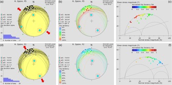
The palaeostress tensor was calculated from 47 VCT and their host planes recorded in the A, B, C and D exposures (Fig. 1d) using the widely used Win-Tensor program (Delvaux, Reference Delvaux2011) (Fig. 5). The four parameters are first estimated with an improved version of the Right Dihedra method, based on Angelier & Mechler (Reference Angelier and Mechler1977). Afterwards, they are more precisely determined with an iterative rotational stress optimization using the default algorithm, i.e. a composite algorithm F5, which minimizes the slip deviation between observed slip line and resolved shear stress and favours slip on the fault planes (Delvaux & Sperner, Reference Delvaux and Sperner2003). In other words, the F5 algorithm tries to find the highest possible slip tendency (Ts), i.e. the ratio of shear stress (τ) to normal stress (σ n) on a plane, as introduced by Morris et al. (Reference Morris, Ferrill and Henderson1996). Therefore, the resolved stress tensor calculated with the F5 algorithm facilitates the slip activation from the dynamic and mechanic perspectives. Although the very low friction of the slip planes does not facilitate the use of the F5 algorithm, this analysis could not be excluded a priori. In addition, the F2 algorithm was used (presented by Angelier (Reference Angelier1975) and mentioned as f2 in Angelier (Reference Angelier and Hancock1994)), which is also provided in the Win-Tensor software and searches only for the dynamic attributes of the slip planes, i.e. the slip vectors of the slip planes under a driving stress tensor based on the Wallace–Bott hypothesis (Wallace, Reference Wallace1951; Bott, Reference Bott1959).
Stress inversion results with F5 (a, b, c) and F2 (d, e, f) algorithms provided by Win–Tensor software (Delvaux, Reference Delvaux2011). Lower–hemisphere, equal–area projections (a, b, d, e), with (a, d) showing the misfit angle histograms, and (b, e) the slip tendency values. (c, f) Mohr diagrams (stresses are of ‘nominal’ values). The crossing line shows the lowest initial friction curve at the frictional angle ϕ = 16.7°.

The F5 solution determines a palaeostress tensor (Fig. 5a, b, c) that has σ 1: 356/58°, σ 2: 245/13°, σ 3: 147/29° and R = 0.38, and the calculated average slip tendency for the input planes is just above that defined by Byerlee’s law (Byerlee, Reference Byerlee1978), i.e. Ts = 0.65. This palaeostress tensor deviates from the Andersonian state of stress, considering that none of its principal stress axes plunges >65° (cf. Lisle et al. Reference Lisle, Orife, Arlegui, Liesa and Srivastava2006), and thus simply defines an inclined stress regime. An interesting issue here is that although the slip planes are of low friction, they are highly facilitated to activate from a mechanical point of view by this driving stress tensor. On the other hand, the F2 algorithm, which considers only the misfit angle (MA) minimization criterion, defines a palaeostress tensor (Figs 5d, e, f) with σ 1: 010/73°, σ 2: 245/10°, σ 3: 153/14° and R = 0.66, which can be considered as an Andersonian tensor. Nonetheless, this tensor calculates much less average slip tendency, i.e. Ts = 0.42, for the input planes, showing that the regional stress regime alone could not have driven the described deformation under the brittle stress regime.
An interesting difference between the F5 and F2 solutions, although not as obvious as the difference between the two calculated slip tendencies, concerns the magnitude of σ 2 with respect to the mean stress (the latter equals (σ 1 + σ 3)/2). More specifically, in the F5 tensor, σ 2 is smaller in magnitude than the mean stress (σ 1 + σ 3)/2 and can therefore be considered to be acting as a relatively extensive stress (Fig. 5c), defining a Radial – Pure Extension (RE-PE) stress regime (stress types according to Tranos et al. Reference Tranos, Kachev and Mountrakis2008). Conversely, in the F2 tensor, σ 2 is greater than the mean stress and in this case can be considered as acting as a relatively compressive stress (Fig. 5f) now defining a Pure Extension – Transtension (PE-TRN) stress regime.
4. Tectonic implications
The deformation of the Arabian platform in the Eastern Province of Saudi Arabia and the area of the Dammam Dome is still not well understood. As the Arabian platform in the Eastern Province is flat and is, in its largest segment, blanketed by loose aeolian sandy material, potential field studies of brittle faulting are difficult. Finally, any knowledge gained from oil exploration is strictly confidential, and therefore unpublished. Such issues have limited our knowledge of faults in the region, and therefore the intraplate deformation and stresses of the region of the Dammam Dome are speculative. Moreover, the exposed mesoscale brittle structures like fractures and discontinuities do not contribute to this knowledge, although some present-day in situ stress measurements indicate that the intraplate stresses with maximum horizontal in situ stress (
 ${\sigma _{\rm{H}}}$
) trending E–W to ENE–WSW, and the minimum horizontal in situ stress (
 ${\sigma _{\rm{h}}}$
) trending N–S to NNW–SSE, are related to Zagros tectonics (Ameen et al. Reference Ameen, Buhidma and Rahim2010; Ameen, Reference Ameen2014). Only the PNU is considered as a possible sign of inception of the Zagros collision in the area during the Oligocene (Weijermars, Reference Weijermars1999), without, however, defining anything about the intraplate stresses and their relationships with the plate boundary stresses along the Zagros orogen.
Instead, by defining the existence of the Rus soft-sediment detachment, the present study indicates an instability in the eastern part of the Arabian platform in the Late Eocene, which could be related to intraplate stresses transferred from plate boundary stresses along the Zagros orogen. However, dynamic analysis of the Rus detachment with the two different algorithms F5 and F2 defines non-Andersonian and Andersonian states of stress, respectively. Unfortunately, the absence of antithetic conjugate slip planes dipping to the SSE introduces significant uncertainties in the determination of the orientation of the stress axes, thus making it impossible to choose which of them is the best explanatory candidate since both can dynamically explain the displacement along the slip planes. The shear to normal stress on a slip plane, i.e. the slip tendency, does not have a direct relationship with the slip preference, in other words, to the theoretical slip direction under a given driving stress tensor (Lisle & Srivastava, Reference Lisle and Srivastava2004; Tranos, Reference Tranos2012). Nonetheless, the F5 algorithm that contains a component of the maximum shear to normal stress ratio for the slip planes (Delvaux & Sperner, Reference Delvaux and Sperner2003; see also http://damiendelvaux.be/Tensor/UserGuides/Win_Tensor-UserGuide_Optimization%20Functions.pdf) provides different resolved stress tensors than those defined by the algorithms solely based on the MA minimization criterion.
In the literature, possible reasons explaining the deviation of the orientation of the principal stress axis from verticality are: (a) the deeper depths away from the Earth’s free surface, (b) the non-horizontal topography, (c) rotation or folding of the area, (d) mechanical inhomogeneities and (e) complex deflection of stress trajectories in the vicinity of large-scale faults or other relatively weak horizons (Lisle et al. Reference Lisle, Orife, Arlegui, Liesa and Srivastava2006). Considering these reasons, the F5 resolved stress tensor might be admissible for the region. Nonetheless, the exposed sedimentary rocks all over the Dammam Dome are almost horizontal, dipping no more than 5°, apart from places where they are steeply dipping due to slumping (Tleel, Reference Tleel1973; Weijermars, Reference Weijermars1999). The region’s topography on a regional scale is flat (see fig. 7 in Weijermars, Reference Weijermars1999). Stratigraphic relationships within the Dammam Dome suggest uplift rates of 7 to 7.5 m/My for most of the Cenozoic (Weijermars, Reference Weijermars1999), implying that the Rus and Dammam sediments have not experienced burial depths of more than 500 m. Finally, the vertical to steeply dipping joints or fractures as recorded by Al-Fahmi (Reference Al-Fahmi2012) and Hariri (Reference Hariri2014), which are opening-mode mostly forming orthogonal sets, and without displaying evidence of shear (Al-Fahmi, Reference Al-Fahmi2012) in the Middle Rus Formation, favour the near-vertical position of the maximum principal stress axis (σ 1) and therefore the Andersonian state of stress. Likewise, the steeply dipping Mode III fractures (i.e. normal faults) reported by Hariri & Abdullatif (Reference Hariri and Abdullatif2005).
Conclusively, in such shallow depths with the near-vertical position of the maximum principal stress axis (σ 1) as defined by the exposed brittle structures of the region as in the region of the Dammam Dome, the arguments supporting the non-Andersonian state of stress cannot be further considered, thus making the F5 stress tensor not admissible for this region. On the other hand, the F2 resolved stress tensor, which was calculated using only the MA minimization criterion, defines an Andersonian stress tensor that better describes the regional stress regime from the geological point of view.
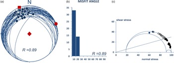
The difference between the non-Andersonian and Andersonian states of stress can be better seen when the stress inversion Tensor Ratio Method (TRM) is applied on the same data (Tranos, Reference Tranos2015), since the latter calculates pure Andersonian stress tensors. The TRM resolved stress tensor (Fig. 6) has σ 1: 159/90°, σ 2: 069/00°, σ 3: 159/00° and R = 0.89, explaining all the fault-slip data with MA ≤ 20° and mean MA (MMA) = 7.2°. It defines a transtension (TRN) stress regime under which σ 2 is compressive, i.e. much greater than the mean stress, and the average slip tendency is even smaller than the F2 solution, i.e. average Ts = 0.3, for the input planes.
Stress inversion results with the application of the TR method (TRM; Tranos, Reference Tranos2015). (a) Equal–area, lower–hemisphere projection; σ 1, σ 2 and σ 3 are shown with solid rhomb, circle and square, respectively, R is stress ratio. (b) Misfit angle histogram. (c) Mohr diagram (stresses are of ‘nominal’ values; see Tranos Reference Tranos2015); blue filled circles show data with Ts ≥ 0.6; open circles show data with Ts < 0.6. The blue crossing line shows the lowest initial friction curve at the frictional angle ϕ = 16.7°.

The Andersonian state of stress, however, does not favour detachment activity in the brittle regime since its vertical maximum principal stress σ 1 forms an obtuse angle with the very gently dipping Rus detachment. This mechanical inconsistency between the Andersonian state of stress and the low-angle normal faults (LANFs) is controversial (e.g. Axen, Reference Axen1992; Scott & Lister, Reference Scott and Lister1992; Abers, Reference Abers2009; Collettini, Reference Collettini2011; Lacombe et al. Reference Lacombe, Jolivet, Le Pourhiet, Lecomte and Mehl2013). Regardless of our ability to explain the frictional slip of low-angle normal faults (LANFs) under an Andersonian state of stress, they are associated with vertical joints and veins which show that detachment activity occurred while the maximum principal stress was nearly vertical (e.g. Collettini & Barchi Reference Collettini and Barchi2002; Skarpelis, Reference Skarpelis2002; Famin et al. Reference Famin, Philippot, Jolivet and Agard2004; Mehl et al. Reference Mehl, Jolivet and Lacombe2005). A fact that allows these detachment faults to be classified as ‘weak’ faults in this sense is that they occur at a large angle (>45°) to the maximum compressive stress σ 1.
According to the Anderson–Byerlee frictional fault mechanics, when the friction coefficient or Ts values ≥ 0.6, any brittle normal fault dipping at high or obtuse angle θ from the vertical maximum principal stress σ 1 is locked (e.g. Anderson, Reference Anderson1951; Byerlee,Reference Byerlee1978; Sibson, Reference Sibson1985; Tranos, Reference Tranos2012). However, Reynolds & Lister (Reference Reynolds and Lister1987) and Axen & Selverstone (Reference Axen and Selverstone1994) argued for a vertical maximum stress axis around LANFs in metamorphic core complexes. Moreover, such flat-lying detachment faults have been recognized in highly extended areas like the western United States (Wernicke, Reference Wernicke1981; Davis et al. Reference Davis, Lister and Reynolds1986) and the Cyclades (Mehl et al. Reference Mehl, Jolivet and Lacombe2005; Lecomte et al. Reference Lecomte, Jolivet, Lacombe, Denèle, Labrousse and Le Pourhiet2010; Lacombe et al. Reference Lacombe, Jolivet, Le Pourhiet, Lecomte and Mehl2013).
Plausible solutions might be that either these LANFs or detachments were initially steep-dipping faults that progressively reoriented passively, being inactive faults (e.g. Proffett, Reference Proffett1977), or the regional stress regime was non-Andersonian outside the fault zone (Spencer & Chase, Reference Spencer and Chase1989; Yin, Reference Yin1989; Parsons &Thompson, Reference Parsons and Thompson1993). However, both solutions are unsuitable in the Dammam Dome case, for the previously described reasons. Likewise, they could not explain a series of cases worldwide, as shown from structural-neotectonic and seismicity studies (e.g. Doser, Reference Doser1987; Morris & Anderson, Reference Morris and Anderson1996; Rietbrock et al. Reference Rietbrock, Tiberi, Scherbaum and Lyon-Caen1996; Abers et al., Reference Abers, Mutter and Fang1997; Bernard et al. Reference Bernard, Briole, Meyer, Lyon-Caen, Gomez, Tiberi, Berge, Cattin, Hatzfeld, Lachet, Lebrun and Stavrakakis1997; Axen et al. Reference Axen, Fletcher, Cowgill, Murphy, Kapp, MacMillan and Aranda-Gómez1999; Skarpelis Reference Skarpelis2002; Mehl et al. Reference Mehl, Jolivet and Lacombe2005; Lecomte et al. Reference Lecomte, Jolivet, Lacombe, Denèle, Labrousse and Le Pourhiet2010; Collettini, Reference Collettini2011; Denèle et al. Reference Denèle, Lecomte, Jolivet, Lacombe, Labrousse, Huet and Le Pourhiet2011; Lacombe et al. Reference Lacombe, Jolivet, Le Pourhiet, Lecomte and Mehl2013).
It seems that the frictional slip on LANFs or detachments requires special conditions to occur which are related to the weakness of the materials or the presence of fluid pressure (Axen & Selverstone, Reference Axen and Selverstone1994). Sibson (Reference Sibson1985) suggests that for reactivation of such faults to occur, either fluid pressures must be high with effective principal stress σ3′ < 0, at least intermittently, or the frictional coefficient must be abnormally low or stress trajectories must deviate markedly from the horizontal and vertical. The evidence supporting the hypothesis for an effectively tensile least principal compressive stress accompanying reactivation should be sought in the form of fault-related hydraulic extension fractures (e.g. Sibson Reference Sibson1981). On the other hand, Axen & Selverstone (Reference Axen and Selverstone1994) suggest that slip can occur along shallow-dipping faults if these faults were pre-existing weakness planes with no cohesive strength under moderate fluid pressure but relatively high differential stress, because the surrounding zone has significant cohesion and fails in transtension.
An alternative model to explain the detachment activity on pre-existing structures has been proposed by Lecomte et al. (Reference Lecomte, Le Pourhiet, Lacombe and Jolivet2011). Contrary to the classical mechanical model, the faults are modelled as thin layers or shear zones, which deform with elasto-plastic rheology (Vermeer, Reference Vermeer1990) rather than as dislocations with frictional properties. This model predicts locking angles (dip angles below which the faults are inactive) which differ in most cases by less than 10° from the classical model, with a significant amount of strain (in the elasto-plastic regime) occurring on badly oriented faults before locking in a strain-hardening regime favoured by compaction of fault gouge.
Considering the above, the activation of the Rus detachment can be explained due to the following reasons or their combinations: (a) the boundary/interface between the Lower and Middle Rus can be considered as a pre-existing weakness plane; (b) the friction is very low or absent and therefore no cohesive strength along this boundary can be considered, as shown by the hydroplastic behaviour of the massive microcrystalline limestone of the Middle Rus; (c) the fact that the effective principal stress axis σ 3′ < 0 as shown by the cm-scale extension fractures filled with calcite similar to geodes or clastic material (Fig. 3d, h) is observed on the R surfaces. These structures are oriented perpendicular to the NNW–SSE extension and can be interpreted as hydraulic extension fractures. Besides, a similar tensile stress regime is also shown by the exposed structures, i.e. joints and fractures that cross-cut the Middle Rus of the Rus Formation (Al-Fahmi, Reference Al-Fahmi2012; Hariri, Reference Hariri2014) and which characterize the brittle regime under the lithification state; (d) the fluid pressure confined along the boundary/interface between the Lower and Middle Rus. These fluids might have accumulated by meteoric water and sedimentary brines in high-salinity basins (Spencer & Welty, Reference Spencer and Welty1986; Wilkins et al. Reference Wilkins, Beane, Heidrick, Beatty and Wilkinson1986; Roddy et al. Reference Roddy, Reynolds, Smith and Ruiz1988) like those formed in sabkha to marine environments dominating the Arabian platform during the Eocene; and (e) the compaction due to the sedimentary loading that facilitates plastic strain on badly oriented faults according to the model of Lecomte (Lecomte et al. Reference Lecomte, Le Pourhiet, Lacombe and Jolivet2011).
Another interesting issue about the driving stresses in the Dammam Dome region is their possible relationship with stresses defined along the plate boundaries, more precisely along the Zagros orogen. The transtension stress regime with vertical maximum principal stress axis σ 1 as described by F2 and TRM stress tensor is in accordance with the present-day stress regime defined from the in situ stress measurements for the Eastern Province region (Ameen et al. Reference Ameen, Buhidma and Rahim2010; Ameen, Reference Ameen2014). Under this stress regime, σ 2 >> mean stress = (σ 1 + σ 3)/2, almost equal to σ 1, having, as a result, to cause compression along the ENE–WSW trend. This compression is very close in trend to the NE–SW compressive stresses under which the main folding phase of the Zagros orogen began to develop toward the Arabian craton forming the ZFB (Lacombe et al. Reference Lacombe, Mouthereau, Kargar and Meyer2006). Therefore, it is logical to consider these ENE–WSW horizontal compressive stresses as the transfer of intraplate stresses from the Zagros orogen due to the inception of the collisional processes during the Late Eocene – Oligocene. In addition, such compressive stresses favour the formation of the Dammam Dome and the uplift of the region, whereas the NNW–SSE extension that is in accordance with the present-day minimum in situ stresses can be considered to represent an orogen-parallel extension since it trends parallel to the Zagros mountain belt. However, the present-day stresses along the Zagros orogen are now NNE–SSW, having changed from NE–SW since the Late Miocene–Pliocene (Lacombe et al. Reference Lacombe, Mouthereau, Kargar and Meyer2006). Therefore, it seems that the present-day intraplate stresses in the Eastern Province of the Arabian platform are rather remnant, residual stresses locked in the rock during the past episodes of tectonic and gravitational stresses related to the Zagros collision and the main folding phase at the regional scale, which gave rise to the ZFB.
The transtension stress regime under which minimum stress axis (σ 3) trends NNW, and the maximum (σ 1) and intermediate (σ 2) principal stresses are of almost equal magnitudes, can lead to a constriction or axially symmetric extension deformation assuming a homogeneous material like that of the massive limestone of the Middle Rus Formation. Such deformation facilitates the stretching and the formation of (a) grooves and cannelures on the Y shears and (b) physiographic features formed by Y and R shears.
The movement along the Rus detachment could not be directly assessed. However, it should be of at least a few hundred metres or possibly of km scale because the VCT structures have been recognized at sites more than a few hundred metres apart from each other and showing constant stretching direction.
5. Conclusions
Odd structures that constitute hydroplastic kinematic indicators, and were previously ignored or falsely interpreted, are described in detail here. They are exposed at the basal part of the Middle Rus Formation above its boundary/interface with the underlying Lower Rus Formation. The majority of structures are translated calcite nodules or geodes that have been eroded out. Their imprints are now fist-sized vugs associated with carrot- or comet-trail imprints (VCT structures). They exist in relation to a principal displacement zone, i.e. the Rus soft-sediment detachment along the boundary/interface of the Lower/Middle Rus. The VCT structures are mainly observed on rock surfaces interpreted as Riedel shears, Y shears and rare P shears in relation to the Rus soft-sediment detachment. The VCT structures define a NNW–SSE-stretching orientation and hundreds of metres to km-scale slip towards the NNW along the detachment. Palaeostress analysis indicates that an Andersonian transtension stress regime, under which the maximum and intermediate principal stress axes are of equal magnitudes, better describes the intraplate stresses of the Dammam Dome region during the Late Eocene and explains the formation of the Dammam Dome and the uplift of the region during the Cenozoic. The stress regime is in accordance with the strike-slip to transtension stress regime defined by the present-day in situ stress measurements in the Eastern Province of Saudi Arabia (Ameen et al. Reference Ameen, Buhidma and Rahim2010; Ameen, Reference Ameen2014).
Moreover, the ENE–WSW horizontal maximum compressive stresses under this transtension fit well with the plate boundary compressive stresses that originated due to collision along the Zagros orogen and the main folding forming the ZFB. Therefore, the soft-sediment structures reflect the instability of the Arabian plate and the transfer of the intraplate stresses of the Zagros orogen to the interior of the subducting or lower Arabian plate in the Late Eocene. Likewise, the Zagros collision was initiated earlier in the Late Eocene and not in Oligocene times, as shown previously by the PNU.
The classical mechanical model does not favour the activation of the Rus detachment under an Andersonian state of stress. However, the activation of the Rus detachment is favoured by factors found herein like the transtensional Andersonian stress regime, the negative effective principal stress σ 3′, the abnormally low frictional coefficient caused by the fluid pressure, and the very low (if not absent) friction that characterizes the soft-sediment deformation.
The present study indicates that it is the soft-sediment structures, rather than the brittle structures, which reflect the instability of the Arabian Platform in the region of the Eastern Province during Late Eocene times. Based on this, the soft-sediment structures better capture and describe the transfer of the plate boundary stresses to the interior of the subducting or lower plate, and thus they are more ‘sensitive stress sensors’ than brittle structures.
Acknowledgements
We greatly appreciate C. Pascal, S. Whattam and an anonymous reviewer for their detailed and patient reviews that considerably improved the original paper, and O. Lacombe for the excellent editorial handling. The first author cordially thanks S. Cain Noltsis, S. Magliveras and P. Neofotistos for proofreading.
Conflicts of interest
None