Introduction
Tropical savannas and forests are generally seen as distinct biomes composed of distinct plant functional types (PFT) and vegetation structure (Furley et al. Reference Furley, Proctor and Ratter1992). Savannas have an open canopy with fire and herbivory considered major drivers of species composition (Hovestadt et al. Reference Hovestadt, Yao and Linsenmair1999, Van Langevelde et al. Reference Langevelde Van, Vijver Van De, Kumar, Koppel van de, Ridder De, Andel Van, Skidmore, Hearne, Stroosnijder, Bond, Prins and Rietkerk2003). Forests have a closed canopy where fire does not easily penetrate and with woody species present being fire sensitive (Torello-Raventos et al. Reference Torello-Raventos, Feldpausch, Veenendaal, Schrodt, Saiz, Domingues, Djagbletey, Ford, Kemp, Marimon, Marimon, Lenza, Ratter, Maracahipes, Sasaki, Sonke, Zapfack, Taedoumg, Villarroel, Schwarz, Quesada, Ishida, Nardoto, Affum-Baffoe, Arroyo, Bowman, Compaore, Davies, Diallo, Fyllas, Gilpin, Hien, Johnson, Killeen, Metcalfe, Miranda, Steininger, Thomson, Sykora, Mougin, Hiernaux, Bird, Grace, Lewis, Phillips and Lloyd2013). Differences in canopy closure with a fire-quenching threshold at around 50% crown cover may result in contrasting pyrogenic (open tree cover) and non-pyrogenic (closed tree cover) biomes (Hennenberg et al. Reference Hennenberg, Fischer, Kouadio, Goetze, Orthmann, Linsenmair, Jeltsch and Porembski2006, Pellegrini et al. Reference Pellegrini, Franco and Hoffmann2016, Ratnam et al. Reference Ratnam, Bond, Fensham, Hoffmann, Archibald, Lehmann, Anderson, Higgins and Sankaran2011). Ecotone vegetation is considered intrinsically unstable and rapidly transforming into either a stable savanna or alternate stable forest state through fire-mediated feedbacks (Hirota et al. Reference Hirota, Holmgren, Van Nes and Scheffer2011, Hoffmann et al. Reference Hoffmann, Geiger, Gotsch, Rossatto, Silva, Lau, Haridasan and Franco2012, Oliveras & Malhi Reference Oliveras and Malhi2016, Pellegrini et al. Reference Pellegrini, Franco and Hoffmann2016, Staver et al. Reference Staver, Archibald and Levin2011). Stands containing mixtures of forest and savanna trees then, as a consequence, are considered fire-degraded and temporary (Aubréville Reference Aubréville1938, Ratnam et al. Reference Ratnam, Bond, Fensham, Hoffmann, Archibald, Lehmann, Anderson, Higgins and Sankaran2011, Stebbing Reference Stebbing1935) but transitional vegetation comprising of a mix of forest and savanna tree species has been reported to persist over decadal timescales (Cuni-Sanchez et al. Reference Cuni-Sanchez, White, Calders, Jeffery, Abernethy, Burt, Disney, Gilpin, Gomez-Dans and Lewis2016, Goetze et al. Reference Goetze, Horsch and Porembski2006). Thus closed-canopy vegetation formations containing an abundance of fire-tolerant canopy tree species may occur naturally, at least under certain conditions. Moreover, in at least one of the classic fire experiments, under a moderate (e.g. early burning) fire regime, many fire-sensitive species were found to persist (Charter & Keay Reference Charter and Keay1960). Thus to simply distinguish between forest and savanna only and to consider transition vegetation to simply be unstable or degraded forest begs for closer scrutiny.
Climate and soil factors are key determinants of vegetation structure (Lloyd et al. Reference Lloyd, Bird, Vellen, Miranda, Veenendaal, Djagbletey, Miranda, Cook and Farquhar2008, Lloyd & Veenendaal Reference Lloyd and Veenendaal2016, Veenendaal et al. Reference Veenendaal, Torello-Raventos, Feldpausch, Domingues, Gerard, Schrodt, Saiz, Quesada, Djagbletey, Ford, Kemp, Marimon, Marimon Junior, Lenza, Ratter, Maracahipes, Sasaki, Sonké, Zapfack, Villarroel, Schwarz, Ishida, Gilpin, Nardoto, Affum-Baffoe, Arroyo, Bloomfield, Gjeca, Compaore, Davies, Diallo, Fyllas, Gignoux, Hien, Johnson, Mougin, Hiernaux, Killeen, Metcalfe, Miranda, Steininger, Sykora, Bird, Grace, Lewis Sl and Lloyd2015, Reference Veenendaal, Torello-Raventos, Miranda, Sato, Oliveras, Van Langevelde, Asner and Lloyd2018). Edaphic properties influence the distribution and structure of tropical woody vegetation types (Dowling et al. Reference Dowling, Webb and Scanlan1986, Goodland & Pollard Reference Goodland and Pollard1973, Trapnell et al. Reference Trapnell, Martin and Allan1950) with soil depth and/or texture and consequently soil water storage an important driver of species composition and stand structure (Keay Reference Keay1960, San Jose & Farinas Reference San Jose and Farinas1983, Swaine Reference Swaine1996, Veenendaal et al. Reference Veenendaal, Swaine, Agyeman, Blay, Abebrese and Mullins1996a, Reference Veenendaal, Swaine, Blay, Yelifari and Mullins1996b). Although in savannas, soil nutrients may be sufficient to potentially sustain forest (Bond Reference Bond2010; Gray & Bond Reference Gray and Bond2015), forest soils are generally of a higher nutrient status than savanna soils under similar climate conditions (Lloyd et al. Reference Lloyd, Bird, Vellen, Miranda, Veenendaal, Djagbletey, Miranda, Cook and Farquhar2008, Quesada et al. Reference Quesada, Phillips, Schwarz, Czimczik, Baker, Patiño, Fyllas, Hodnett, Herrera, Almeida, Alvarez Dávila, Arneth, Arroyo, Chao, Dezzeo, Erwin, Di Fiore, Higuchi, Honorio Coronado, Jimenez, Killeen, Lezama, Lloyd, López-González, Luizao, Malhi, Monteagudo, Neill, Núñez Vargas, Paiva, Peacock, Peñuela, Peña Cruz, Pitman, Priante Filho, Prieto, Ramírez, Rudas, Salomao, Santos, Schmerler, Silva, Silveira, Vásquez, Vieira, Terborgh and Lloyd2012, Ruggiero et al. Reference Ruggiero, Batalha, Pivello and Meirelles2002). Of particular interest is the combined soil available water and potassium (CWAK) hypothesis (Lloyd et al. Reference Lloyd, Domingues, Schrodt, Ishida, Feldpausch, Saiz, Quesada, Schwarz and Torello-Raventos2015) which suggests that soil water availability and the nutrient potassium together can explain vegetation structural transitions in woody vegetation.
In this paper, we closely examine variation in the structural parameters of woody vegetation in a forest–savanna boundary in Ghana, West Africa, investigating links between the vegetation composition in terms of woody PFTs and the vegetation structure in a forest–savanna mosaic. We also test the hypothesis that savanna and transitional species can co-occur in at least some closed vegetation formations. We also investigate long-term changes and fire incidence for different vegetation structural type, testing the hypothesis that many differences in vegetation structure can be simply attributed to variation in soil characteristics.
Methods
Study site
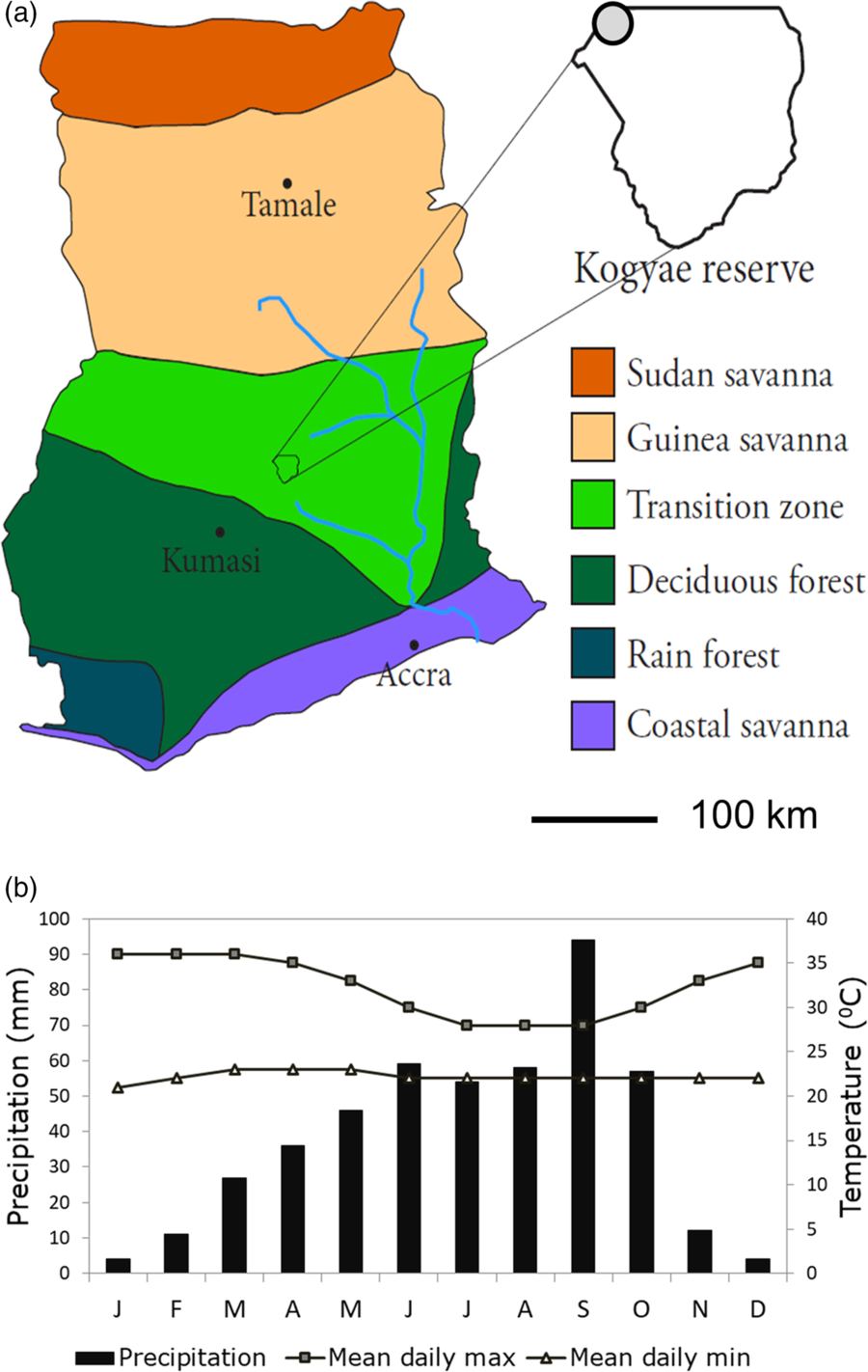
We conducted the study in the Kogyae Strict Nature Reserve (KSNR; Figure 1a) in the Ashanti Region of Ghana (7°15′52′′N, 1°04′47′′W). KSNR was established in the 1960s as a barrier reserve between the Guinea Savanna Zone in the north and the Deciduous Forest Zone in the south (Hawthorne Reference Hawthorne1995, Janssen et al. Reference Janssen, Ametsitsi, Collins, Adu-Bredu, Oliveras, Edward, Mitchard and Veenendaal2018). KSNR covers an area of 330 km2. Average rainfall is ~1.36 m year−1 and the average annual temperature is 28°C with little season variation (Figure 1b: Wildlife Department Accra 1994). Rainfall distribution is seasonal with a distinct wet and dry season. Heavy rains fall between May and October with varied intensity, followed by a dry season from December to March. Long-term rainfall above the escarpment in Central Ghana has declined by 10–20% compared with the period 1950–1970 (Owusu & Waylen Reference Owusu and Waylen2009). Presently KSNR regionally experiences annual, mostly early wildfires, mostly the result of hunting/poaching and agriculture. Since 2004, fire has also been used as a tool to improve grazing resources for wildlife in the north-east section of the park. The structural vegetation types within the KSNR range from closed forests to open woodlands. Much of the forest vegetation was, however, chopped down in the late 1980s and early 1990s in the run-up to the gazetting of the strict conservation status of the park (Janssen et al. Reference Janssen, Ametsitsi, Collins, Adu-Bredu, Oliveras, Edward, Mitchard and Veenendaal2018).
Map of Ghana showing the different vegetation zones and location of the Kogyae Strict Nature Reserve. Vegetation zonation adapted from Yengoh et al. (Reference Yengoh, Armah, Onumah and Odoi2010). The grey circle indicates the location of the study site (a). Yearly rainfall and temperature distribution for the Kogyae Strict Nature Reserve (b) (McSweeney et al. Reference McSweeney, New, Lizcano and Lu2010; Wildlife Department Accra 1994).

The KSNR vegetation also has a human footprint, with there being some record of occupation for the 19th and 20th century. For example, pottery can be found (Wildlife Department Accra 1994) and transitional woodland patterns have sometimes been linked to past agricultural activity. Nevertheless, detectable features of past human settlements such as forest patches consisting of Terminalia schimperi (Hochst. ex Hutch. & Dalziel) Gere & Boatwr (syn. Anogeissus leicocarpa (DC.) Guill. & Perr.) which typically persist for decades after village abandonment (Hopkins Reference Hopkins1965, Sobey Reference Sobey1978) were not detected in the study area.
A total of 35 plots of 20 × 20 m were established in the north-east corner of the park (Figure 1a). This plot size was considered to be small enough to allow for a homogeneous vegetation structure but still large enough to obtain a representative sample of the dominant tree species composition (with there usually being more than 15 trees with a diameter at breast height (dbh) of 2.5 cm or more in each plot). All plots were located in an area where no recent human disturbances such as logging were detectable. The plots were distributed in patches of varying tree cover across the naturally occurring vegetation mosaic and first classified a priori by eye as savanna-like (woody vegetation with incomplete canopy closure and a herb layer of C4 grasses), forest-like (woody vegetation with complete canopy closure and a sparse herb layer of mainly C3 forbs and C3 grasses), and ‘intermediate’. Fifteen plots were established in the savanna-like vegetation, 10 plots in the forest-like vegetation, and 10 plots in semi-closed ‘intermediate’ vegetation. All plots were located a maximum distance of 3.0 km from each other to allow for likely similar historical fire patterns. Also plots were only established in flat areas of the landscape (0–3% slope, estimated by eye) to avoid surface hydrological processes and the influence of catena.
Vegetation parameters
In each plot, diameter and height were measured of trees with a diameter ≥ 2.5 dbh. Trees were identified at species level. The crown area of each tree was calculated from crown diameter measured on two perpendicular axes. Total canopy area was calculated by summing up crown areas. Basal area was calculated as the sum of basal area of all individual trees in a plot. Canopy area index (CAI) was determined by dividing total crown area by the area of the plot. Height of all trees > 10 cm dbh was measured with a laser rangefinder (TruPulse® 200, Laser Technology Inc.). Hemispheric photographs, to determine woody leaf area index (LAI), were taken using a Nikon E4500 camera with fisheye lens, mounted at 1 m height. Photographs were underexposed by two stops to enhance contrast (Woodgate et al. Reference Woodgate, Soto-Berelov, Suarez, Jones, Hill, Wilkes, Axelsson, Haywood and Mellor2012, Zhang et al. Reference Zhang, Chen and Miller2005). LAI was determined using Gap Light Analyser imaging software with contrast settings determined by three independent observers (Frazer et al. Reference Frazer, Canham and Lertzman1999, Promis et al. Reference Promis, Gärtner, Butler-Manning, Durán-Rangel, Reif, Cruz and Hernández2011).
Tree classification, biomass calculation and structural vegetation plot clustering
Based on information on species habitat and/or distribution as taken from Keay (Reference Keay1989), Hawthorne (Reference Hawthorne1995) and Hawthorne & Jongkind (Reference Hawthorne and Jongkind2006) all species in the study were classified a priori as savanna-affiliated (S), forest-affiliated trees (F) or non-specialized (N) – the latter species having been reported as regularly occurring in both forest and savanna. Estimates of above-ground woody biomass (AGB) for each plot were calculated using a generic allometric equation for tropical trees (Chave et al. Reference Chave, Réjou-Méchain, Búrquez, Chidumayo, Colgan, Delitti, Duque, Eid, Fearnside, Goodman and Henry2014).
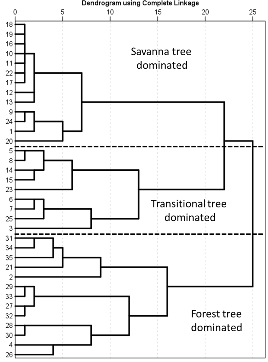
To investigate similarity in PFT composition, plots were clustered on the basis of the contribution of the PFTs to the total crown area in the plot using all trees ≥ 2.5 cm dbh, using SPSS version 23.0 (complete linkage and single Euclidian distance to emphasize plot differences). For the second classification, CAI, AGB, average canopy height (H), the 0.95 quantile of average canopy height, H*: calculated as H* = H + 1.645 σ where σ = the plot standard deviation of tree height (Hyndman & Fan Reference Hyndman and Fan1996) for trees ≥ 10 cm dbh. This clustering allows for a classification in structural vegetation types (VST) as defined by Torello-Raventos et al. (Reference Torello-Raventos, Feldpausch, Veenendaal, Schrodt, Saiz, Domingues, Djagbletey, Ford, Kemp, Marimon, Marimon, Lenza, Ratter, Maracahipes, Sasaki, Sonke, Zapfack, Taedoumg, Villarroel, Schwarz, Quesada, Ishida, Nardoto, Affum-Baffoe, Arroyo, Bowman, Compaore, Davies, Diallo, Fyllas, Gilpin, Hien, Johnson, Killeen, Metcalfe, Miranda, Steininger, Thomson, Sykora, Mougin, Hiernaux, Bird, Grace, Lewis, Phillips and Lloyd2013).
Soil chemical and physical analyses
In September 2014 composite soil samples were taken in the middle of the growing season at depth intervals of 0–10, 10–20, 20–40, 40–60, 60–80 and 80–100 cm with a cylindrical soil auger at the centre of a plot and in the four quadrants. Samples were air dried before laboratory analysis. Total N and total P were determined according to Novozamsky et al. (Reference Novozamsky, Houba, Van Eck and Van Vark1983). Available P (P-Olsen) was determined according to Olsen (Reference Olsen1954). The cation exchange capacity (CEC) and exchangeable K, Ca and Mg were determined after extraction with unbuffered 0.01 M BaCl2 (Gillman Reference Gillman1979). Percentage organic matter (OM) was determined by loss on ignition. Soil pH was determined in H2O (1:2.5). All soil nutrient data are expressed on a volume basis as nutrients available in 1 m3 using bulk density measurements taken at 20-cm intervals from the surface to 100 cm depth using soil pits.
Soil moisture content (MC) was determined by weighing soil samples (taken in September 2014 and additionally in the dry season in January 2015) in the field with a digital balance of precision ± 0.01 g in situ. The water mass was determined after drying at 80oC to constant weight. Percentage soil moisture content was expressed in volume by multiplying the gravimetric water content with bulk density. Particle size analysis for composite samples representing from the top 20 cm was as per the Boyoucos method (Gee & Bauder Reference Gee, Bauder and Klute1986).
Soil depth (d) in each plot was determined by digging a 1.5 × 2.0-m soil pit to the ferricrete layer or, on occasion, sandstone layer. In six representative plots, a complete soil description and classification was undertaken with layers of different appearance, thickness and properties arising from various soil-forming processes being recorded. The resulting information was used in conjunction with the laboratory analyses to classify soil types according to the World Resource Base soil classification scheme (IUSS Working Group WRB 2006) with pit descriptions deposited in the Dryad Digital Repository. For the remaining 29 plots, soils were classified by eye by a local pedologist using information acquired from six pits that had been analysed in detail.
Fire occurrence and vegetation cover change
The occurrence of fire was estimated by the fire return time (period 2000–2014) on the basis of the MODIS Burned Area Product (MCD45A1; Roy et al. Reference Roy, Boschetti, Justice and Ju2008). As this product has a spatial resolution of 500 × 500 m and fire may still be patchy within a landscape, whether a specific plot actually would have burned in a given year cannot be determined precisely. We therefore define a fire occurrence as one in the vicinity of the plot (but not whether the plot has actually burned) and quantified as the fire return time of the pixel in which the plot was located.
To evaluate any link between fire history and vegetation change, vegetation cover was determined by calculation of the averaged Normalised Vegetation Index (NDVI) change over the period 1984–2015 in four steps. We first used NDVI derived from Landsat TM (21 November 1984 and 22 November 1990), Landsat ETM+ (15 November 2002) and Landsat OLI (27 November 2015) at a resolution of 30 × 30 m. The NDVI from 1984, 1990 and 2002 was then cross-calibrated to the NDVI of 2015 correcting for sensor differences (Mitchard et al. Reference Mitchard, Saatchi, Gerard, Lewis and Meir2009). NDVI trends over the period were subsequently determined for each plot using linear regression across the four data points for NDVI over time and determining the slope of the regression line.
Statistical analyses
Statistical analyses were undertaken with SPSS version 23 unless stated otherwise. Comparisons of structural properties between plots were done with a single ANOVA and post hoc Tukey test. Data were sometimes log-transformed to ensure normality of the residuals and homogeneity of variances. If this proved insufficient non-parametric tests were applied. To test for differences in tree heights of the tallest trees a general linear model assuming normal error distribution (GLM) was used. GLMs were also used to test whether there were differences in soil nutrients, soil depth and other environmental resources between the PFTs or VSTs. Each GLM was followed by a post hoc Tukey test to determine the differences between the PFT or VST groupings. For the analysis of NDVI cover change trends we used a GLM with PFT or VST groupings as a factor and CAI as a covariate to compensate for the fact that CAI shows a saturating relationship with increasing CAI (Janssen et al. Reference Janssen, Ametsitsi, Collins, Adu-Bredu, Oliveras, Edward, Mitchard and Veenendaal2018).
Vegetation structural properties were first correlated with soil physical and chemical properties using Kendall’s non-parametric rank correlation test. Ordinary Least Squares (OLS) models were used to quantify relationships between BA, CAI and AGB and the measured soil parameters, selecting the minimum adequate model based as that with the lowest Bayes information criterion (BIC) which has a stricter penalty associated with additional terms as compared to the Akaike information criterion (AIC) thus reducing any chance of overfitting (Schwarz Reference Schwarz1978). These analyses were undertaken using the R statistical platform using the dredge function within the MuMIn package (Bartoń Reference Bartoń2013) with the simplest model within two units of the lowest BIC model chosen (Aho et al. Reference Aho, Derryberry and Peterson2014).
Results
Classifying vegetation with plant functional or structural properties
As detailed in Appendix 1, 56 tree species were found across the 35 study plots of which 19 were classified as savanna-affiliated (S), 26 as forest-affiliated (F) and 11 as non-specialized (N).
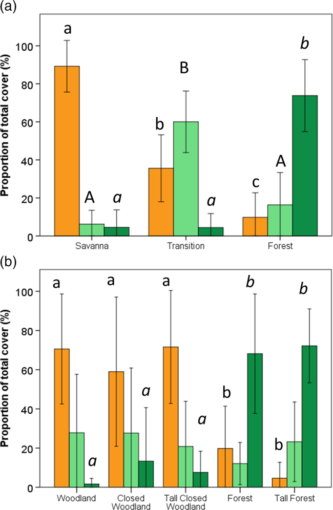
Classification of plots on the basis of PFT cover contribution resulted in three clusters which, on the basis of their species composition as weighted by canopy cover, were classified as either savanna (89% ± 3.6% (mean ± SE) ST dominance), transitional (60% ± 5.4% N dominance) or forest (74% ± 5.5% F dominance; Figure 2a, Appendix 2). Frequently occurring forest (F) tree species included Ceiba pentandra, Didymosalpinx abbeokutae, Manilkara obovata and Sterculia tragacantha. Dominant savanna (S) trees included Terminalia glaucescens and Pterocarpus erinaceus. Typically ubiquitous non-selective (N) trees include Bridelia micrantha, Lannea nigritana, Margaritaria discoidea and Pouteria alnifolia.
Percentage composition of forest, savanna and non-specialized tree species by crown area in plots at the Kogyae Strict Nature Reserve, Ghana, grouped on the basis of plant functional types (a) and grouped on the basis of the vegetation structural characteristics (b). Orange bars represent savanna trees, light green bars non-specialized trees and dark green bars forest trees. Different letters (small caps, capital, italics) indicate significant differences of the tree types between the classes (one-way ANOVA post hoc Tukey test; P < 0.05). Error bars denote ± 1 SD.
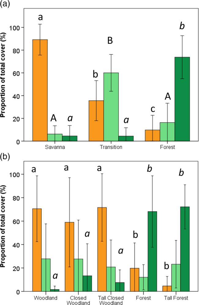
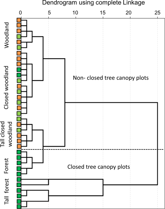
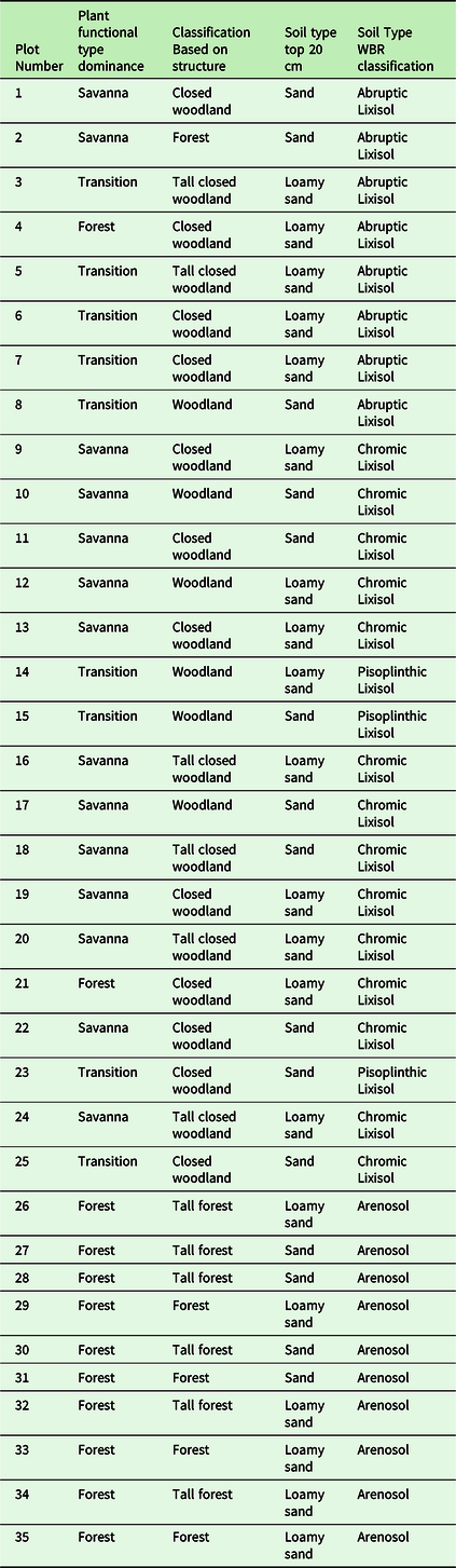
Alternatively, classifying on the basis of stand structural parameters resulted in five clusters viz. woodland, closed woodland, tall closed woodland, forest and tall forest (Figure 2b, 3). Woodland (including closed and tall closed) was on average dominated by S-species (59–75%), while F-species dominated the forest and tall forest classifications (on average 68–72%), also being much rarer in other VSTs (max 15%) and almost absent in woodlands. N-species were on average more equally distributed among VSTs (12–28%; Figure 2b). Variation in dominance of PFTs within individual structural groupings was, however, large. For example the woodland grouping contained both S- and N-dominated stands within the closed woodlands grouping encompassing stands dominated by all three PFT (Figure 3). In closed-canopy-forest and tall-forest plots the species PFT classification was always F-affiliated.
Clustering of the plots at the Kogyae Strict Nature Reserve, Ghana, into vegetation structural types. Typology follows Torello-Raventos et al. (Reference Torello-Raventos, Feldpausch, Veenendaal, Schrodt, Saiz, Domingues, Djagbletey, Ford, Kemp, Marimon, Marimon, Lenza, Ratter, Maracahipes, Sasaki, Sonke, Zapfack, Taedoumg, Villarroel, Schwarz, Quesada, Ishida, Nardoto, Affum-Baffoe, Arroyo, Bowman, Compaore, Davies, Diallo, Fyllas, Gilpin, Hien, Johnson, Killeen, Metcalfe, Miranda, Steininger, Thomson, Sykora, Mougin, Hiernaux, Bird, Grace, Lewis, Phillips and Lloyd2013) (all trees ≥ 10 cm dbh). Squares on the y axis indentify the plant functional type classification of the same plots (orange = savanna tree dominated, light green = non-specialized tree dominated, dark green = forest tree dominated) (see also Appendix 2).
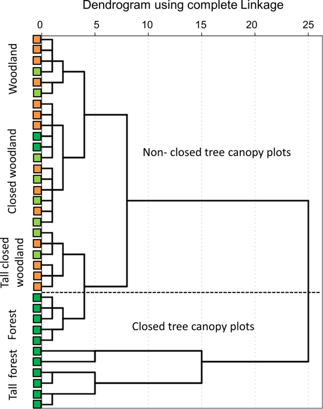
Forest species in woodland and closed woodlands were typically of smaller-than-average stature than is typical for this PFT (although sometimes up to ~25 m tall), with the most common F-species in woodland being Sterculia tragacantha Lindl., Vitex grandiflora Gurke and Kigelia africana (Lam.) Benth. S-trees were found only in low numbers in forest and tall forest, but within tall closed woodland and (tall) forest patches, several tall-statured S-affiliated specimens such as Terminalia schimperi and Khaya senegalensis Desr. (height up to 30 m) were found. N-species were found in all five VSTs, with this group including taller species such as Afzelia africana Sm. and Lannea nigritana (Scot-Elliot) Keay. Comparing the PFT classification with the VST classification, S-dominated plots were generally classified as woodlands up to tall closed woodlands, N-dominated plots as woodlands to tall closed woodlands, and F-dominated plots as closed woodlands, forest or tall forest. Smaller trees and shrubs (viz. dbh 2.5–5 cm) were absent in woodland but constituted 5% of all trees in VST in the other woodland classes and 15% in the forest classes (data not shown).
Variation in quantitative vegetation structural properties
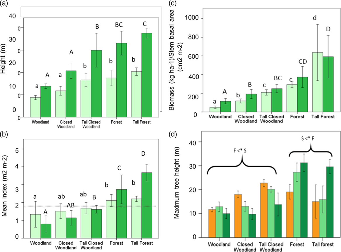
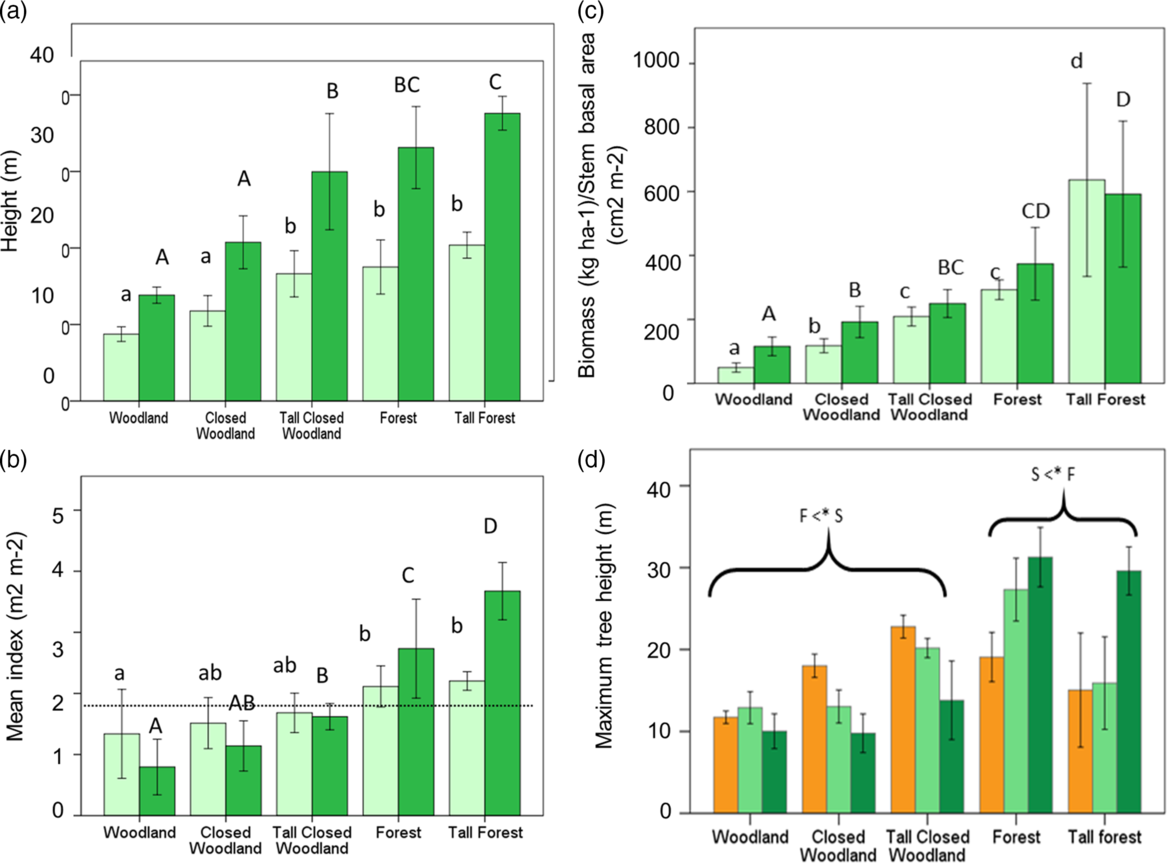
Variation in structural properties for the five VST categories is shown in Figure 4. Average canopy height and 95% quantile height were lowest for woodlands and closed woodland with both these VSTs being significantly shorter than tall closed woodland and forest (Figure 4a). Leaf area index varied from 1.3 m2 m−2 to 2.2 m2 m−2 in tall forests with complete canopy closure – taken here as occurring at a LAI of 1.7 to 1.8 m2 m−2 equating to a projected crown cover of 60% – observed for the forest and tall forest plots (Figure 4b). CAI varied between 0.8 m2 m−2 in woodlands to 3.7 m2 m−2 in tall forest (Figure 4b). AGB increased from around 100 Mg ha−1 in woodlands to over 200 Mg ha−1 in forest with a large increase to near 600 Mg ha−1 for tall forests (Figure 4c). Average maximum height achieved by individual trees, being the tallest tree recorded for each PFT, in each plot is shown in Figure 4d. Average maximum height differed significantly across the different VSTs with a significant interaction between PFT and VST (GLM; P < 0.001): F-species were significantly shorter (P < 0.05) than S-species in woodlands (including the closed and tall closed woodlands), but S-species were significantly shorter than F-species in the forest and tall-forest plots. On the other hand, maximum tree height for N-species did not vary significantly across VSTs (Figure 4d).
Variation of structural traits across the vegetation structural types of the plots at the Kogyae Strict Nature Reserve, Ghana. Average canopy height (light green bars); 95% quantile height (dark green bars) (a); leaf area index (light green bars) crown area index (dark green bars) (b), the dotted line indicates a threshold level where the canopy is considered closed. Above-ground biomass (light green bars) and stem basal area (dark green bars) (c). Different letters in a, b and c indicate significant differences between the classes (one-way ANOVA post hoc Tukey test. P < 0.05) (after logtransforming data for ABG and BA). Maximum tree height per plant functional type (d) (orange bars savanna trees, light green bars non-specialized trees and dark green bars forest trees). Brackets in (d) indicate that savanna trees (S) are significantly taller in woodlands (all types) compared with forest trees (F) and forest trees are significantly taller in forest types. Non-specialized trees are intermediate in all cases. Error bars denote ± 1 SD.
Fire occurrence near plots and vegetation cover change
Fires were assessed over the period 2000–2015, with most fires occurring in the period after 2005 (with as a result thus in recent years a higher frequency). For the whole period average fire frequency in the vicinity of the plots was 0.35 ± 0.08 year−1 (mean ± SE) for woodlands, 0.30 ± 0.05 year−1 for closed woodland and tall closed woodland plots, 0.29 ± 0.03 year−1 for forest plots and 0.26 ± 0.03 year−1 for tall forest plots with only woodlands being significantly different from tall forest plots (one way ANOVA; F = 2.98, P < 0.35 with post hoc Tukey test).
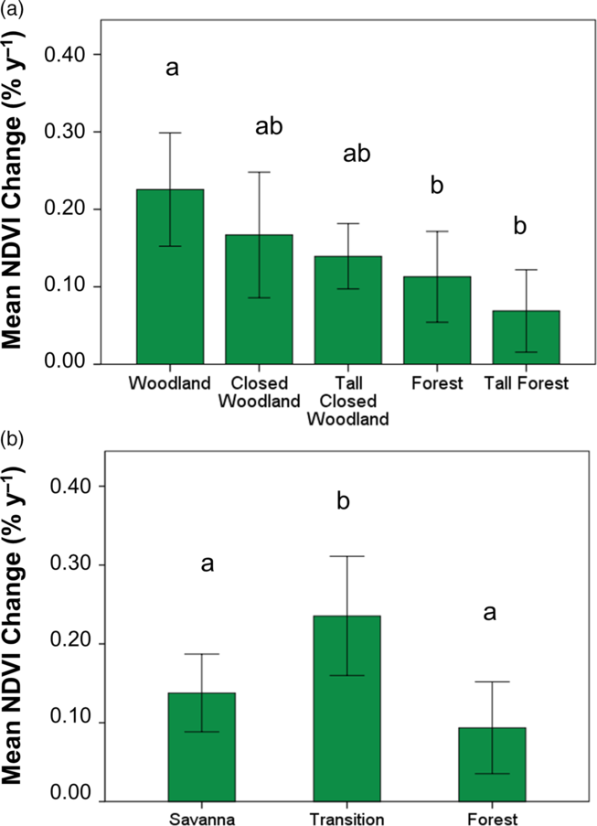
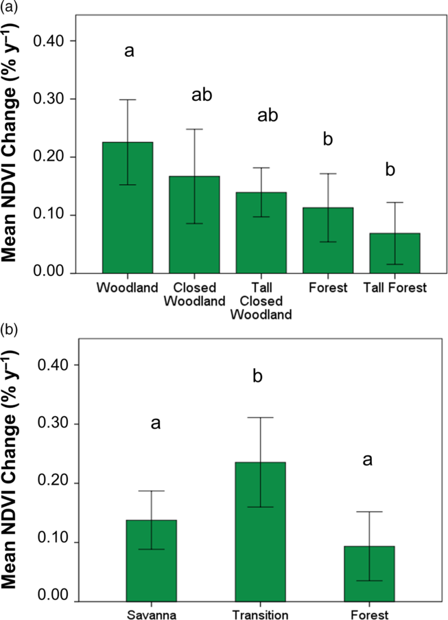
Including CAI as (non-significant) covariate, the long-term vegetation cover trend, measured through NDVI change between 1984 and 2015, was significantly different between VSTs (data analysed with a single ANOVA; F (4, 30) = 4.68, P < 0.005). All VSTs showed an increase in NDVI over the period 1984–2005 (Figure 5a) with the highest rate of increase in woodland being 0.23% year−1. Closed woodlands showed an average increase of 0.11% year−1, with the slowest rate of increase being for the tall forest plots (0.08% year−1). Cover increase of PFT classified vegetation types was also significantly different between plots (CAI again included as a covariate but now significant; F (1,31) =5.06, P < 0.032; PFT F (1,32) = 1.44 P < 0.001) and showed a significantly larger increase of 0.22% ± 0.02% year−1 (marginal mean ± SE) in N-dominated plots than for S-dominated and F-dominated plots for which the rates of increase were 0.11% ± 0.02% year−1 and 0.13% ± 0.02% year−1 respectively (Figure 5b).
Mean NDVI change in the different vegetation structural types (a) and Plant functional type dominated (b) plots in the Kogyae Strict Nature Reserve, Ghana, over the period 1984–2015. Letters indicate significant differences between the types. (a) One-way ANOVA post hoc Tukey test; P > 005. Error bars denote ± 1 SD. (b) GLM with CAI as covariate. Means are marginal means with a test of contrasts P > 005. Error bars denote ± 1 SE.
Soil physical and chemical parameters and vegetation structural classification
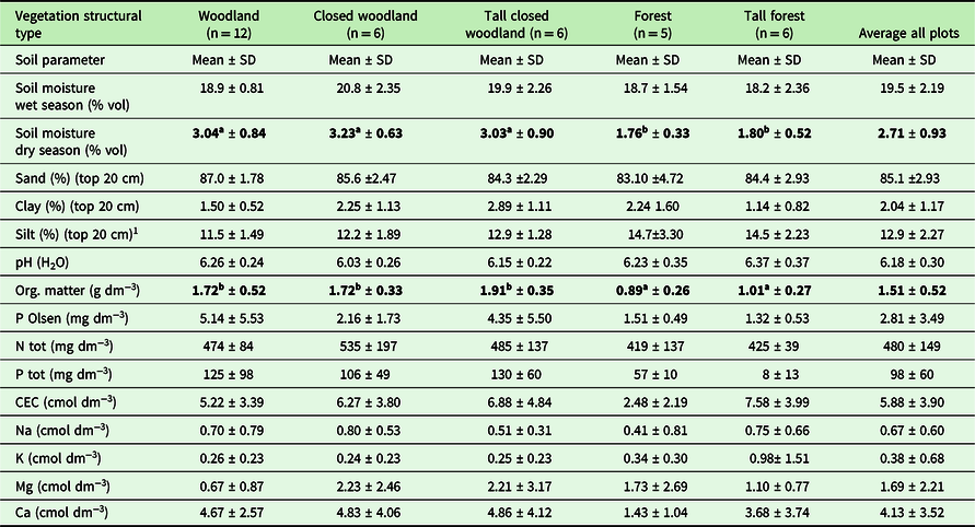
All soils were of a high sand content (Appendix 3) with woodlands and closed woodlands generally found on Lixisols, and forests mostly on Arenosols. Maximum soil depth ranged from 1.0 m and 2.6 m and, although varying significantly between VSTs (GLM analysis; F 4, 30 = 2.93, P < 0.04), with differences not significant in a post hoc test, but significant (P < 0.013) with soil depths for forest and tall forest grouped VSTs (average 2.08 ± 0.26 m) versus woodlands and closed woodlands grouped VSTs (average 1.71 ± 0.43 m).
Soil physical and chemical data integrated across the upper 1-m profile for each plot are shown in Table 1. No significant differences were found in particle size between the different VSTs in the first 20 cm of the soil. Across all plots, increased silt fractions occurred at the expense of lower sand fractions, and with the clay fractions (always less than 0.05 g g−1) also being slightly greater in siltier soils (Appendix 4).
Soil parameters in the vegetation structural type plots at Kogyae, Ghana. Soil Moisture Organic matter, pH (H2O) and soil nutrients are averaged over 1 m depth. Particle size analysis was done over the top 20 cm. All values are calculated per volume unless indicated otherwise. Parameters for which significant differences were found are in bold. Superscripts indicate differences at P < 0.05; Single ANOVA with post hoc Tukey test

Soil pH (H2O) values ranged from 6.1–6.4 and did not differ across VSTs (one way ANOVA, P < 0.179). Soil nutrients were variable and did not differ systematically according to VST. Although wet-season volumetric soil moisture content (θ V) did not differ significantly between VSTs (GLM F4,30 = 6.77, P < 0.099) when sampled in the dry season, soils under forest VSTs had more depleted soil moisture (θ V ~ 0.018) as compared with the woodland VSTs (θ V ~ 0.031) with these differences being significant at P < 0.001.
Soil physical and chemical parameters and vegetation structural variation
Using non-parametric Kendall’s τ to probe associations between the vegetation structural properties of canopy height, crown area index (CAI), leaf area index (LAI), above-ground woody biomass (AGB) and basal area (BA) with environmental and edaphic conditions (Table 2), significant bivariate correlations were found for all four canopy structure metrics and with the frequency of fire occurrence in the vicinity of the study plots (P < 0.05), and with correlations of both LAI and AGB with soil depth (P < 0.01 in both cases). Soil silt content was also positively correlated with all of canopy height (P < 0.05), CAI (P < 0.01) and AGB (P < 0.01). There were also negative correlations between all four structural metrics with organic matter content (P < 0.01) and dry-season soil moisture content and negative correlations for some or all of the canopy structural metrics with total N, extractable P and total P.
Correlations between vegetation structural parameters and environmental conditions and resources for the plots in Kogyae Strict Nature Reserve, Ghana. Numbers represent Kendall’s τ coefficient (n = 35; *, P < 0.05; **, P < 0.01) Can Hgt = Canopy height; CAI = Crown area index; LAI = Leaf area index; AGB = above ground biomass; Fire = Fire occurrence in the vicinity of the plot; MC WS = Moisture content Wet season profile; MC DS Moisture content dry season profile; S depth = Soil profile depth; % Sand top 20 cm; % Clay top 20 cm; % Silt top 20 cm; OM = organic matter; P Olson extr.; N total; P total; CEC = Cation exchange capacity; Na = Na extractable; K = K extractable; Mg =Mg extractable and Ca = Ca extractable. Parameters for which significant differences were found are in bold

Organic matter content correlated positively with fire frequency in the vicinity of a plot (P < 0.01) as well as soil water content in the dry season (P < 0.01), also showing positive relationships with total nitrogen (P < 0.05) and both total and exchangeable phosphorus (P < 0.01). Soil depth and exchangeable potassium (Kex) were also positively correlated (P < 0.01).
Soil factors as predictors of vegetation structure
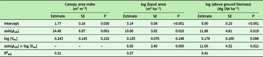
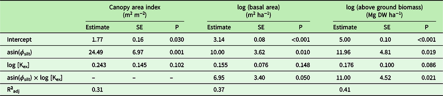
Ignoring VFT or PFT classification and simply testing plot-level soil parameters directly against the associated CAI, BA or AGB (with the latter two measures being log-transformed due to their heteroscedasticity: Figure 4), both silt fraction ϕ silt and log exchangeable potassium [Kex] emerged as the best predictors in all three cases (Table 3) and with a positive interaction between ϕ silt and log [Kex] for both BA (R2 = 0.37) and AGB (R2 = 0.41), but not for CAI (R2 = 0.31) also found.
Estimates for ordinary least square models relating variation for selected structural variables (basal area and canopy area index) to selected soil variables of the plots in Kogyae Strict Nature Reserve, Ghana. Models were selected on the basis of their Bayes Information Criterion (BIC). Symbols and units: ϕ silt = silt fraction (dimensionless); [Kex] = soil exchangeable potassium (cmol m−3). Also given is the coefficient of determination adjusted according to the statistic based on the number of independent variables in the model. In all cases the independent variables have been centred on their mean
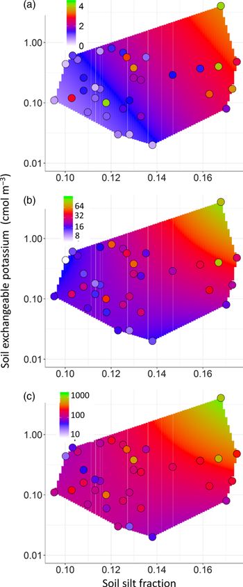
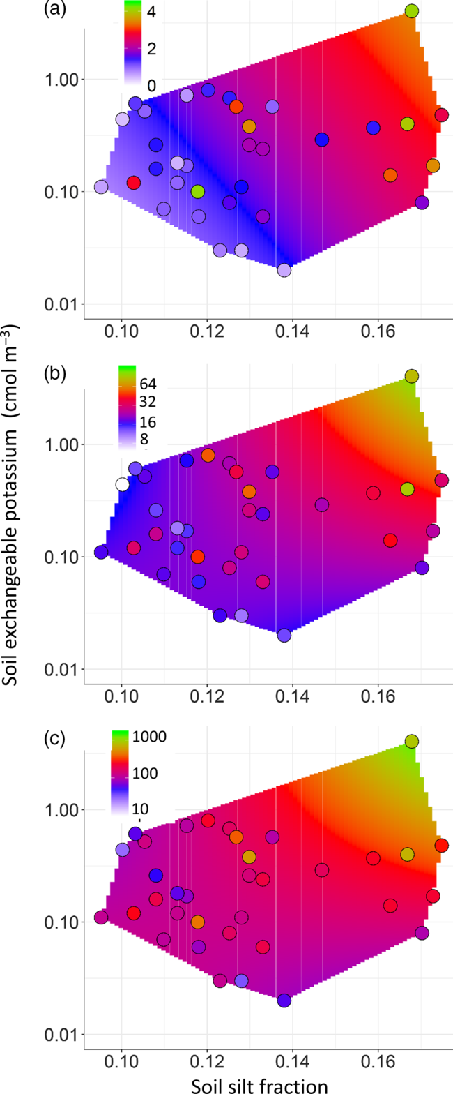
The nature of the predicted responses is shown in the form of a ‘heat plot’ in Figure 6 with the observed values also shown. All three metrics of canopy structure showed similar responses with maximum values found when high [Kex] and high ϕ silt occur simultaneously. The same data are also shown in the more conventional form of plots of predicted vs. observed values in Appendix 5 with symbols coloured according to report fire frequency as well.
Modelled responses to variations in soil silt fraction, ϕ silt, and exchangeable potassium concentration, [Kex]. (a) canopy area index (m2 m−2), (b) stand basal area (m2 m−1), (c) above-ground biomass (Mg DW ha−1) for plots at the Kogyae Strict Nature Reserve, Ghana. Observations are shown as circles underlain by a ‘heat map’ of the modelled response across the dataset [Kex]; ϕ silt domain as represented by a convex hull (Rodrıguez Casal & Pateiro López Reference Rodríguez Casal and Pateiro López2010).
Discussion
Vegetation composition versus structure
Our main objective here has been to establish the link between plant functional type trees (savanna, transitional and forest species) and vegetation structure in vegetation patches in a forest–savanna mosaic in Ghana (Figure 4). Although our plots were smaller than most, the structural parameters quantified in our 400-m2 plot encompassed variation generally observed in forest–savanna transitions (Mitchard et al. Reference Mitchard, Saatchi, Lewis, Feldpausch, Woodhouse, Sonké, Rowland and Meir2011, Veenendaal et al. Reference Veenendaal, Torello-Raventos, Feldpausch, Domingues, Gerard, Schrodt, Saiz, Quesada, Djagbletey, Ford, Kemp, Marimon, Marimon Junior, Lenza, Ratter, Maracahipes, Sasaki, Sonké, Zapfack, Villarroel, Schwarz, Ishida, Gilpin, Nardoto, Affum-Baffoe, Arroyo, Bloomfield, Gjeca, Compaore, Davies, Diallo, Fyllas, Gignoux, Hien, Johnson, Mougin, Hiernaux, Killeen, Metcalfe, Miranda, Steininger, Sykora, Bird, Grace, Lewis Sl and Lloyd2015). There were some high biomass plots of above 600 Mg ha−1 in tall forest patches. Such variation may be expected in plots of smaller scale as used in our study (Mitchard et al. Reference Mitchard, Saatchi, Lewis, Feldpausch, Woodhouse, Sonké, Rowland and Meir2011, Veenendaal et al. Reference Veenendaal, Torello-Raventos, Feldpausch, Domingues, Gerard, Schrodt, Saiz, Quesada, Djagbletey, Ford, Kemp, Marimon, Marimon Junior, Lenza, Ratter, Maracahipes, Sasaki, Sonké, Zapfack, Villarroel, Schwarz, Ishida, Gilpin, Nardoto, Affum-Baffoe, Arroyo, Bloomfield, Gjeca, Compaore, Davies, Diallo, Fyllas, Gignoux, Hien, Johnson, Mougin, Hiernaux, Killeen, Metcalfe, Miranda, Steininger, Sykora, Bird, Grace, Lewis Sl and Lloyd2015).
At this spatial scale of investigation, plot classification according to plant functional types (PFTs) showed a clear separation between S-species-dominated plots, N-species-dominated plots and F-species-dominated plots (Figure 2). This is not surprising as trees often demonstrate clustered distributions at relatively small (400 m2) spatial scales, especially when all tree size classes are included (Couteron & Kokou Reference Couteron and Kokou1997). The distribution of PFTs across the various vegetation structural types (VST) did, however, show a mixing of species. Generally S-trees were mostly limited to woodland (including closed and tall closed) VSTs, with F-trees predominantly occurring in forest VSTs; but with N-trees were found in all VSTs as might be expected from their a priori assigned ubiquitous position (Figure 2). Nevertheless, F-trees occurred in significant numbers in (tall) closed woodlands and S-trees in forest plots. Thus at our spatial scale of investigation forest and savanna PFTs are not exclusively separated. Some mixing of S- and F-species has been recognized before in West African transitional vegetation (Asare Reference Asare1962, Charter & Keay Reference Charter and Keay1960, Hopkins Reference Hopkins1965, Schrodt et al. Reference Schrodt, Domingues, Feldpausch, Saiz, Quesada, Schwarz, Ishida, Compaore, Diallo, Djagbletey, Hien, Sonké, Toedoumg, Zapfack, Hiernaux, Mougin, Bird, Grace, Lewis, Veenendaal and Lloyd2015, Torello-Raventos et al. Reference Torello-Raventos, Feldpausch, Veenendaal, Schrodt, Saiz, Domingues, Djagbletey, Ford, Kemp, Marimon, Marimon, Lenza, Ratter, Maracahipes, Sasaki, Sonke, Zapfack, Taedoumg, Villarroel, Schwarz, Quesada, Ishida, Nardoto, Affum-Baffoe, Arroyo, Bowman, Compaore, Davies, Diallo, Fyllas, Gilpin, Hien, Johnson, Killeen, Metcalfe, Miranda, Steininger, Thomson, Sykora, Mougin, Hiernaux, Bird, Grace, Lewis, Phillips and Lloyd2013) and in both over- and understorey (Armani et al. Reference Armani, Van Langevelde, Tomlinson, Adu-Bredu, Djagbletey and Veenendaal2018), although this has, at least in some cases, been interpreted as a forest degradation response (Ratnam et al. Reference Ratnam, Bond, Fensham, Hoffmann, Archibald, Lehmann, Anderson, Higgins and Sankaran2011).
The structural classification employed here has allowed comparisons of how key vegetation characteristics such as cover and biomass vary between the VSTs, also allowing us to quantify how the different PFTs may contribute to the various different structures of the stands. For example, in the more open woodland plots dominated by S- and N-species, forest trees are almost entirely lacking. F-species increase in dominance as canopy closure occurs (Figure 2b and 3). This is likely due to the selective pressure of fire for recruitment of forest tree seedlings with canopy closure (Armani et al. Reference Armani, Van Langevelde, Tomlinson, Adu-Bredu, Djagbletey and Veenendaal2018, Boonman et al. Reference Boonman, van Langevelde, Oliveras, Couédon, Luijken, Martini and Veenendaal2019, Cardoso et al. Reference Cardoso, Medina-Vega, Malhi, Adu-Bredu, Ametsitsi, Djagbletey, Van Langevelde, Veenendaal and Oliveras2016, Issifu et al. Reference Issifu, Ametsitsi, Vries De, Djagbletey, Adu-Bredu, Vergeer Langevelde Van and Veenendaal2019).
In the forest plots, presumably better growth conditions have allowed F-trees on average to achieve greater heights than S-trees (Figure 4) although individual savanna trees, particularly Terminalia schimperi and Khaya senegalensis were observed to sometimes attain a forest tree stature with heights of up to 30 m. These predominantly savanna species are often mentioned as pioneer species preceding forest expansion into savanna (Hennenberg et al. Reference Hennenberg, Goetze, Minden, Traore and Porembski2005, Nansen et al. Reference Nansen, Tchabi and Meikle2001). Tall S-trees may also persist in forests long after forest expansion has taken place (Mitchard et al. Reference Mitchard, Saatchi, Lewis, Feldpausch, Woodhouse, Sonké, Rowland and Meir2011) explaining part of the mixing of F- and S-tree species in the larger size classes.
Across all plots in the study area we found a small increase in tree cover over time to have occurred with an average NDVI increment of 0.15% year−1 (Figure 5), this being equivalent to a LAI increment of ~0.01 year−1 or 0.3 units over the 30-y period (Janssen et al. Reference Janssen, Ametsitsi, Collins, Adu-Bredu, Oliveras, Edward, Mitchard and Veenendaal2018). Such slow rates of increase are difficult to detect at short timescales but provide an indication that canopy closure is increasing. The lowest rate of increase in NDVI was for the tall forest plots, but as the relationship between tree cover (e.g. CAI) and NDVI and vegetation cover saturates at CAI > 2.5 (Janssen et al. Reference Janssen, Ametsitsi, Collins, Adu-Bredu, Oliveras, Edward, Mitchard and Veenendaal2018, Mitchard et al. Reference Mitchard, Saatchi, Gerard, Lewis and Meir2009) canopy cover increase based on NDVI increment may have been underestimated for the forest formations. Interestingly, stands dominated by N-tree species showed the highest NDVI increase. Though undoubtedly a heterogenous group, N-species probably have particular traits of a greater plasticity than is the case of F- or N- species, enabling them to persist in variable environments such as forest–savanna ecotones where, for West Africa at least they are commonly observed (Hennenberg et al. Reference Hennenberg, Goetze, Minden, Traore and Porembski2005, Nansen et al. Reference Nansen, Tchabi and Meikle2001).
In this context it is interesting to speculate on how ongoing increases in CO2 may be playing a role in driving the observed slow canopy cover increase. A continuing global increase in CO2 may be playing a role in driving the observed slow canopy cover increase. In tropical trees intrinsic water use efficiency increases have been demonstrated to occur at a rate of 10% or more per 50 years (Sleen et al. Reference Sleen van der, Groenendijk, Vlam, Anten, Boom, Bongers Pons, Terburg and Zuidema2015) potentially compensating for the observed reduction of annual rainfall (Owusu & Waylen Reference Owusu and Waylen2009) in the study area.
A high fire incidence in our study area does not seem to have prevented a gradual woody cover increase, although it may well have just slowed it down: as, for example, our average NDVI increase is at 0.15% year−1 much slower than the ~1% year−1 reported for a forest–savanna transition in Central Africa (1985–2006) where fire incidence had decreased by 30% (Mitchard et al. Reference Mitchard, Saatchi, Lewis, Feldpausch, Woodhouse, Sonké, Rowland and Meir2011). Nevertheless, we do also note that the Cameroon transition also has higher precipitation and greater exchangeable soil K concentrations (Veenendaal et al. Reference Veenendaal, Torello-Raventos, Feldpausch, Domingues, Gerard, Schrodt, Saiz, Quesada, Djagbletey, Ford, Kemp, Marimon, Marimon Junior, Lenza, Ratter, Maracahipes, Sasaki, Sonké, Zapfack, Villarroel, Schwarz, Ishida, Gilpin, Nardoto, Affum-Baffoe, Arroyo, Bloomfield, Gjeca, Compaore, Davies, Diallo, Fyllas, Gignoux, Hien, Johnson, Mougin, Hiernaux, Killeen, Metcalfe, Miranda, Steininger, Sykora, Bird, Grace, Lewis Sl and Lloyd2015). Fire may also influence species selection through recruitment (Armani et al. Reference Armani, Van Langevelde, Tomlinson, Adu-Bredu, Djagbletey and Veenendaal2018, Cardoso et al. Reference Cardoso, Medina-Vega, Malhi, Adu-Bredu, Ametsitsi, Djagbletey, Van Langevelde, Veenendaal and Oliveras2016, Issifu et al. Reference Issifu, Ametsitsi, Vries De, Djagbletey, Adu-Bredu, Vergeer Langevelde Van and Veenendaal2019, Swaine Reference Swaine1992).
Drivers of observed woody cover patterns – fire
According to the Alternative Stable State paradigm, a large emphasis is put on the role of fire in causing unstable transitional vegetation forms which rapidly tend towards either forest or savanna (Hirota et al. Reference Hirota, Holmgren, Van Nes and Scheffer2011, Lehmann et al. Reference Lehmann, Anderson, Sankaran, Higgins, Archibald, Hoffmann, Hanan, Williams, Fensham, Felfili, Hutley, Ratnam, San Jose, Montes, Franklin, Russell-Smith, Ryan, Durigan, Hiernaux, Haidar, Bowman and Bond2014). But interestingly, from this study and others, what actually seems to be happening is a longer-term persistence or slow change (at least at decadal timescales) of intermediate vegetation types in many places (Cuni-Sanchez et al. Reference Cuni-Sanchez, White, Calders, Jeffery, Abernethy, Burt, Disney, Gilpin, Gomez-Dans and Lewis2016, Goetze et al. Reference Goetze, Horsch and Porembski2006). Notwithstanding this, in vegetation types where edaphic conditions are not sufficient to permit canopy closure, there is a strong correlation with fire frequency (Table 2), which is, itself, likely to have influenced canopy cover (for a quantitative analysis of this process see Veenendaal et al. Reference Veenendaal, Torello-Raventos, Miranda, Sato, Oliveras, Van Langevelde, Asner and Lloyd2018). Nevertheless, using the mean fire frequency estimates available here, less than 25% of the data set variation in CAI could be explained by variation in fire frequency (OLS: R2= 0.21, P < 0.005), this being much less than the variation accountable for by the soil properties of Table 3. More detailed observations of fire behaviour in different vegetation structural types in our study area are needed to better understand the relationship between closing cover, fire effects and recruitment opportunities of savanna, forest and non-specialist PFTs in forest–savanna ecotones, especially as regards their interactions with soil physical and chemical properties.
Drivers of observed woody cover patterns – soils
Soil physical and chemical characteristics have already been documented to influence vegetation structure as well as species composition in the study region (Asare Reference Asare1962, Markham & Babbedge Reference Markham and Babbedge1979, Swaine et al. Reference Swaine, Hall and Lock1976). Although there were significant correlations between vegetation structural parameters and soil nutrients, once grouped together we found no large differences between VSTs in nutrient status in our site (Table 1). Nevertheless, organic matter was higher underneath the more open vegetation types, possibly related to accumulation of oxidation resistant carbon of pyrogenic origin or directly related to soil characteristics not measured (Saiz et al. Reference Saiz, Bird, Domingues, Schrodt, Schwarz, Feldpausch, Veenendaal, Djagbletey, Hien, Compaore, Diallo and Lloyd2012).
Although there is some evidence for soil nutrients being co-determinant of the positioning of the forest boundary globally (Veenendaal et al. Reference Veenendaal, Torello-Raventos, Feldpausch, Domingues, Gerard, Schrodt, Saiz, Quesada, Djagbletey, Ford, Kemp, Marimon, Marimon Junior, Lenza, Ratter, Maracahipes, Sasaki, Sonké, Zapfack, Villarroel, Schwarz, Ishida, Gilpin, Nardoto, Affum-Baffoe, Arroyo, Bloomfield, Gjeca, Compaore, Davies, Diallo, Fyllas, Gignoux, Hien, Johnson, Mougin, Hiernaux, Killeen, Metcalfe, Miranda, Steininger, Sykora, Bird, Grace, Lewis Sl and Lloyd2015), the variation in our nutrient measurements between our VST structural groupings did not show significant differences. Nevertheless, when variation in CAI, BA and AGB were considered across the data set as whole, significant relationships involving [K]ex and silt fraction were observed (Table 3). These associations are consistent with the Combined Water and Potassium (CWAK) hypothesis of Lloyd et al. (Reference Lloyd, Domingues, Schrodt, Ishida, Feldpausch, Saiz, Quesada, Schwarz and Torello-Raventos2015) as originally developed in South America. That hypothesis supposes that potassium is a critical nutrient for plant function and growth, especially in water-limited environments where water content of the rooting zone is also important. The latter should be dependent on both rooting depth and soil texture, and according to the models of Table 3 for the very sandy soils of the study area here it seems that relatively minor changes in silt content may be of critical importance. A rough estimate of the likely magnitude of any silt effect can be obtained using the moisture pedo-transfer function of Oliveira et al. (Reference Oliveira, Ribeiro, Jacomine, Rodrigues and Marques2002) which, developed in the semi-arid region of north-east Brazil, is one of the few available that calculates plant available water (PAW) as a function of all silt, clay and sand fractions (Tomasella & Hodnett Reference Tomasella and Hodnett2004). The Oliveira et al. (Reference Oliveira, Ribeiro, Jacomine, Rodrigues and Marques2002) equation also requires an estimate of soil bulk density ρ and, taking our study average of ρ = 1.51 Mg m−3, then with the silt/sand/clay associations of Appendix 4 we obtain for ϕ silt = 0.10 g g−1 an associated PAW of ~0.035 m3 m−3. But for ϕ silt = 0.15 g g−1 the same equation gives PAW ≅ 0.048 m3 m−3. Thus for the coarsely textured soils encountered here an increase in silt fraction of 5% (in absolute terms) might reasonably be expected to result in an increase in PAW of over 30% (in relative terms). Or put another way, integrated over a 2-m depth profile then a soil with a silt fraction of 0.15 g g−1 can potentially store nearly 1.0 m of H2O, but with a silt fraction of 0.10 then the equivalent amount is only about 0.7 m H2O: this difference of about 0.3 m H2O equating to about 1-mo wet-season rainfall (Figure 1b).
In addition to this soil texture effect, impenetrable layers such as ferricretes may obstruct the downward drainage of groundwater (Batjes Reference Batjes1996). In our study area such impermeable layers generally occurred, but for forest soils these were found on average almost 40 cm deeper than woodland plots. A deeper soil profile for forest soils should thus allow for a larger volume of stored water, this then amplifying the silt effect on PAW per unit volume as discussed above. Together these effects could shorten the period of complete depletion of soil water in the upper profile in the dry season by almost 1 mo (Huttel Reference Huttel1975, Veenendaal et al. Reference Veenendaal, Swaine, Blay, Yelifari and Mullins1996b). Soil depth variation such as found by us is already well known to strongly influence tropical vegetation structure (Hiernaux et al. Reference Hiernaux, Diarra, Trichon, Mougin, Soumaguel and Baup2009, Keay Reference Keay1960; Lloyd et al. Reference Lloyd, Domingues, Schrodt, Ishida, Feldpausch, Saiz, Quesada, Schwarz and Torello-Raventos2015, Markham & Babbedge Reference Markham and Babbedge1979, Moore & Attwell Reference Moore and Attwell1999, San José & Farinas Reference San Jose and Farinas1983), with Hartemink & Huting (Reference Hartemink and Huting2008) also noting that small variations in silt content are strongly associated with relatively large changes in the physical and chemical properties of South African Arenosols. Large-scale global analyses considering soils only in terms of their surface-layer sand and carbon contents (Lehmann et al. Reference Lehmann, Anderson, Sankaran, Higgins, Archibald, Hoffmann, Hanan, Williams, Fensham, Felfili, Hutley, Ratnam, San Jose, Montes, Franklin, Russell-Smith, Ryan, Durigan, Hiernaux, Haidar, Bowman and Bond2014) must by necessity ignore such subtle but important variation in soil properties which are no doubt important in influencing tropical vegetation structure across a range of scales.
Conclusion
We aimed to look at variation in vegetation structure and plant functional type composition within a forest–savanna transition zone as related to fire frequency and soil physical and chemical properties. We found evidence for soil-available-water-related parameters, silt content, soil depth and exchangeable potassium to all be playing a role in patch distribution and PFT composition. We did not find support for a bimodal system of fire-prone vegetation consisting of fire-tolerant savanna tree species and fire-suppressed vegetation consisting of fire-sensitive forest tree species as proposed in ASS theory. Rather our ecotonal mosaic consisted of a range of plots of varying canopy cover and with these plots also varying in their relative abundances of savanna, non-specialist and forest species.
Acknowledgements
This paper is dedicated to the memory of Mr Ntim Gyakari who assisted with his extensive botanical knowledge. We thank the Wildlife Division of the Forestry Commission of Ghana for permission to work in the Kogyae Strict Nature Reserve. Our appreciation also goes to the Park Manager, Mr Dwoben Nyantakyi, and his staff at Dome Camp, particularly Isaac Sarpong, Kwaku Yinye and Yaw Agyeman. Elmar Veenendaal and George Ametsitsi were partially funded by the EU KP7 GEOCARBON project (contract number 283080). Jon Lloyd and Vincent Logah received support through Royal Society – DFID (Africa capacity building initiative programme) and with Jon Lloyd also being supported by a Royal Society Wolfson fellowship.
List of tree species in the study plots in the Kogyae Strict Nature Reserve and their division in Plant functional type (F = forest tree; S = savanna tree; N = non-specialized tree)
See main text for further explanation

*Previously Anogeissus Leiocarpus (DC.) Guill. & Perr. (Maurin et al. Reference Maurin, Gere, van der Bank and Boatwright2017)
Clustering of the sampled plots into Plant functional types dominated plot types based on cover (all trees ≥ 2.5 cm dbh). Number on the y axis refers to the plot numbers
Classification of vegetation patches in the study area and soil classification
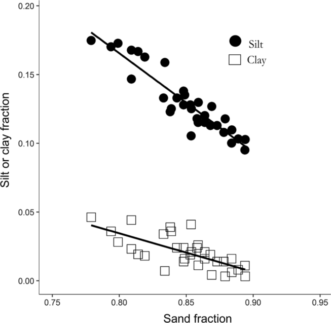
The relationship between sand, silt and clay fractions across the study sites. For silt fraction vs. sand fraction, the OLS regression equation is y = 0.394 – 0.387x (r 2 = 0.86) and for the clay fraction vs. the sand fraction the equation is y = 0.173 – 0.150x (r 2 = 0.48).
Appendix 5.
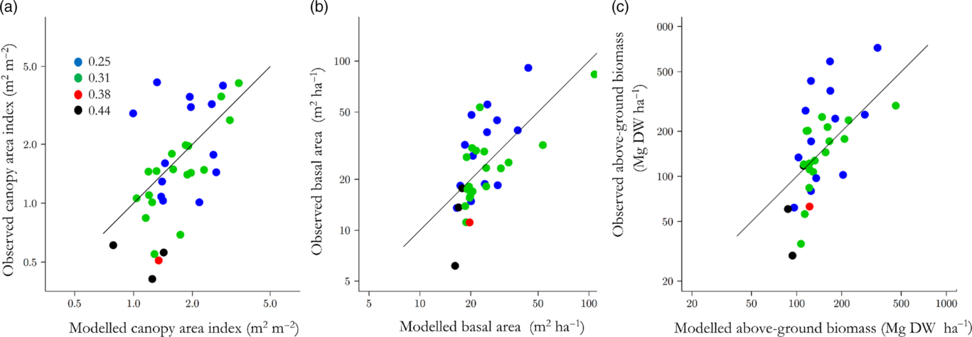
Predictive ability of the models of Table 3. (a) canopy area index, (b) stand basal area (m2 ha−1), (c) above-ground biomass. Symbols are colour coded according to MODIS Burned Area Product derived fire frequency (a−1) for the period 2000–2014 as detailed in panel (a).