1 Introduction
Hydrodynamic lift is the motion of a particle transverse to the streamlines of the imposed flow and the direction of any body force on the particle. It results from the stresses on the particle caused by fluid inertia when the particle Reynolds number is finite. Hydrodynamic lift plays an important role in separation processes such as microfluidic focusing (see Masaeli et al.
Reference Masaeli, Sollier, Amini, Mao, Camacho, Doshi, Mitragotri, Alexeev and Di Carlo2012) and cross-flow filtration (see Drew, Schonberg & Belfort Reference Drew, Schonberg and Belfort1991). While there is extensive literature analysing the lift on spherical particles (see Saffman Reference Saffman1965; Drew Reference Drew1988; McLaughlin Reference McLaughlin1991, Reference McLaughlin1993; Cherukat & McLaughlin Reference Cherukat and McLaughlin1994), relatively little is known about the lift on non-spherical particles. To gain insight into the role of non-sphericity, we derive the lift velocity of a neutrally buoyant high-aspect-ratio cylindrical fibre in a wall-bounded simple shear flow at small, but finite, particle Reynolds number
 $Re=\unicode[STIX]{x1D70C}\dot{\unicode[STIX]{x1D6FE}}l^{2}/\unicode[STIX]{x1D707}$
. Here,
 $l$
is the fibre half-length,
 $\unicode[STIX]{x1D70C}$
is the fluid density,
 $\dot{\unicode[STIX]{x1D6FE}}$
is the shear rate and
 $\unicode[STIX]{x1D707}$
is the viscosity of the fluid. In addition to providing a large contrast to the commonly studied spherical shape, the choice of a fibre allows the use of slender-body theory to describe the flow induced by the fibre, facilitating a quasi-analytical treatment.
Much is known about the hydrodynamic lift on a spherical particle in simple shear flow at small, but non-zero, particle Reynolds number. This lift requires breaking the symmetry of the flow to allow cross-streamline motion. This is achieved by either a body force acting on the particle parallel to the flow direction or a nearby wall. Saffman (Reference Saffman1965) calculated the lift on a sphere in an unbounded shear flow induced by a body force parallel to the streamlines for the case in which the relative velocity due to the body force is much smaller than the imposed shear velocity,
 $\dot{\unicode[STIX]{x1D6FE}}a$
, where
 $a$
is the sphere radius. McLaughlin (Reference McLaughlin1991) generalized this investigation to cover all ratios of the relative velocity and shear velocity. The nature of the analysis for the lift on a particle in the presence of a wall depends on the relative magnitude of the separation from the wall
 $h^{\ast }$
and the Oseen length
 $L_{0}=[\unicode[STIX]{x1D707}/(\unicode[STIX]{x1D70C}\dot{\unicode[STIX]{x1D6FE}})]^{1/2}$
. McLaughlin (Reference McLaughlin1993) studied hydrodynamic lift on spheres at separations comparable to or larger than the Oseen length. This outer analysis involves a singular perturbation analysis that includes a viscous-dominated inner region spanning distances of
 $O(a)$
from the particle and an outer region at separations of
 $O(L_{0})$
where inertial and viscous effects are comparable. However, when the particle is closer to the wall than the Oseen length, the inertial effects can be treated as a regular perturbation from the Stokes flow solution. This inner analysis was carried out by Cherukat & McLaughlin (Reference Cherukat and McLaughlin1994) to evaluate the lift force on spheres. The special case of this result, corresponding to no force along the streamlines, can be used in conjunction with appropriate Stokes flow resistance functions to evaluate the lift velocity of a neutrally buoyant particle. The lift velocity is expected to exhibit very different qualitative and quantitative behaviour due to non-sphericity. This will be especially pronounced in the inner analysis where the fibre geometry has close interaction with the wall. Thus, the focus of this study will be on fibres in the inner region,
 $h^{\ast }\ll L_{0}$
, where a regular perturbation analysis in terms of
 $Re$
is applicable.
The study of the lift on non-spherical particles is very limited compared to the literature available on the lift on spheres. One of the earliest treatments of non-spherical shapes was carried out by Harper & Chang (Reference Harper and Chang1968) who calculated the lift force on three-dimensional bodies in unbounded shear flow in the strong shear limit of Saffman (Reference Saffman1965). Shin, Koch & Subramanian (Reference Shin, Koch and Subramanian2009) studied the lift on a fibre due to a body-force-induced relative velocity and a weak, unbounded shear flow. Numerical studies of the lift-induced trajectories of an elliptical particle have been carried out by Feng, Hu & Joseph (Reference Feng, Hu and Joseph1994) in Couette and Poiseuille flows, considering both neutrally buoyant and sedimenting particles. Qi (Reference Qi1999) numerically studied the lift of rectangular particles. However, there is no analytical treatment of the lift on a force-free fibre. Neither is there any literature available for the hydrodynamic lift of a particle with high aspect ratio (fibre) as a function of the distance from the wall in the presence of a shear flow.
Hydrodynamic lift can play an important role in separating particles of different types and in separating particles from fluid. A common method of separating particles in microchannels is to allow hydrodynamic lift to cause different types of particles to migrate to different positions in the channel. A bifurcation in the channel can then be used to harvest the desired particle type. While such separations have conventionally been based on particle size, Masaeli et al. (Reference Masaeli, Sollier, Amini, Mao, Camacho, Doshi, Mitragotri, Alexeev and Di Carlo2012) have demonstrated experimentally that particle shape plays an important role. In cross-flow filtration, a suspension of particles flows through a channel with porous walls, while fluid filtrate is drawn out through the walls. A major advantage of cross-flow filtration is that the shearing motion helps to limit the formation of a filter cake of particles at the porous membrane surface. Belfort and Drew and co-investigators (see Drew Reference Drew1988; Drew et al. Reference Drew, Schonberg and Belfort1991; Belfort, Davis & Zydney Reference Belfort, Davis and Zydney1994) have argued that hydrodynamic lift, in addition to hydrodynamic diffusion and Brownian diffusion, helps to limit the particle concentration at the membrane surface. Many targets for such separation processes have non-spherical prolate shapes, including biological particles such as bacteria and viruses as well as cellulose fibres of current interest in the production of biofuels. Thus understanding the hydrodynamic behaviour of non-spherical particles will go a long way in improving their filtration in industrial and laboratory settings.
The order of magnitude of the lift velocity of a neutrally buoyant sphere in a shear flow near a wall at small Reynolds number can be understood in a simple way. The characteristic Stokes fluid velocity disturbance in the vicinity of a sphere is
 $\dot{\unicode[STIX]{x1D6FE}}a$
. However, any cross-stream motion of a particle in Stokes flow would violate Stokes flow reversibility. Thus, the lift velocity is the result of fluid inertia, which is quantified by the particle Reynolds number
 $Re_{a}=\unicode[STIX]{x1D70C}\dot{\unicode[STIX]{x1D6FE}}a^{2}/\unicode[STIX]{x1D707}$
. The lift velocity of a sphere is thus proportional to
 $\dot{\unicode[STIX]{x1D6FE}}aRe_{a}=\unicode[STIX]{x1D70C}\dot{\unicode[STIX]{x1D6FE}}^{2}a^{3}/\unicode[STIX]{x1D707}$
.
One can estimate some properties of non-spherical particles in low-Reynolds-number flows as those associated with an equivalent sphere. For example, a common means of estimating the drag on an object in Stokes flow is as the drag on a circumscribing sphere. However, we will see that the lift on a slender fibre at small but finite Reynolds number differs in order of magnitude from that of a circumscribing sphere, and furthermore the dependence of lift on separation from the wall is qualitatively different for fibres and spheres. One important reason for this difference is the role that fibre rotation plays in the lift. A fibre rotates in a periodic motion through a Jeffery orbit (see Jeffery Reference Jeffery1922) spending most of its time near the flow direction and a shorter time flipping through other orientations. Since the fluid velocity disturbance made when the fibre is nearly aligned with the flow direction is much smaller than while it is flipping, its lift behaviour does not resemble that of any equivalent sphere.
Since the lift velocity of a fibre depends on its orientation, a specification of the time-dependent orientation of the fibre is required to predict its spatial migration. In Stokes flow, a fibre rotates periodically in time in one of a set of Jeffery orbits parameterized by the orbit constant
 $C$
. At small but finite Reynolds numbers, Subramanian & Koch (Reference Subramanian and Koch2005) showed that the fibre spirals gradually through orbits and eventually rotates in the
 $C=\infty$
orbit corresponding to orientations within the flow-gradient plane. This has been verified by lattice Boltzmann simulations carried out by Rosén, Lundell & Aidun (Reference Rosén, Lundell and Aidun2014). A linear stability analysis of particle motion in the
 $C=\infty$
orbit for arbitrary aspect ratio at small
 $Re$
by Einarsson et al. (Reference Einarsson, Candelier, Lundell, Angilella and Mehlig2015a
) confirms the predicted slender fibre dynamics. The prediction by Subramanian & Koch (Reference Subramanian and Koch2005) of migration across orbits has been extended to finite-aspect-ratio spheroids by Einarsson et al. (Reference Einarsson, Candelier, Lundell, Angilella and Mehlig2015b
) and Dabade, Marath & Subramanian (Reference Dabade, Marath and Subramanian2016), thereby validating the original result. Thus, we will consider the time-averaged lift that occurs when a fibre has been in the shear flow long enough to reach the
 $C=\infty$
orbit.
The lift velocity of a fibre that does not make contact with the wall but is within the viscous-dominated region, i.e.
 $l<h^{\ast }\ll L_{0}$
, can be determined using a regular perturbation analysis for
 $Re\ll 1$
. In carrying out this analysis we will use the generalized reciprocal theorem to avoid the expensive evaluation of the order Reynolds flow field. This enables the
 $O(Re)$
fibre velocity to be related to a volume integral involving the Stokes fluid velocity field and a comparison field driven by a fibre with a unit force acting perpendicular to the wall. The Stokes flow field consists of the imposed shear flow and a disturbance flow created by the fibre and its hydrodynamic interaction with the wall. The disturbance velocity field due to the particle is represented by a line of Stokeslets distributed along the particle axis. The force distribution on the particle is evaluated by solving the integral equations of the slender-body theory, developed by Batchelor (Reference Batchelor1970), under the simplifying assumption of high aspect ratio. The hydrodynamic interaction of the fibre with the wall is included by using, for each Stokeslet distributed along the fibre, a set of image singularities which Blake & Chwang (Reference Blake and Chwang1974) demonstrated will satisfy the no-slip boundary condition. The high aspect ratio allows expansion in terms of
 $\unicode[STIX]{x1D716}=1/(\ln 2\unicode[STIX]{x1D705})$
, which is the small parameter, with
 $\unicode[STIX]{x1D705}=l/a$
being the aspect ratio. We retain terms of
 $O(\unicode[STIX]{x1D716})$
and
 $O(\unicode[STIX]{x1D716}^{2})$
in this study.
While a sphere makes contact with a wall at only one separation
 $h^{\ast }=a$
and has zero lift velocity owing to lubrication forces at this separation, a fibre can contact the wall for
 $a<h^{\ast }<l$
and we will see that its lift velocity is non-zero in this range. As first observed experimentally by Stover & Cohen (Reference Stover and Cohen1990), the edge of a fibre in Stokes flow with
 $a<h^{\ast }<l$
makes a solid-body contact with the wall. To span the range of behaviours that can arise due to fibre–wall friction, we will consider the two extreme cases of a frictionless contact and a no-slip sticking contact. In both cases, the resulting contact force pushes the fibre away from the wall and shifts its orientation towards smaller
 $C$
, corresponding to migration away from the flow-gradient plane, in a dynamic motion the authors referred to as pole vaulting. We will show that the coupling of pole vaulting with the fluid-inertia-induced orientational changes predicted by Subramanian & Koch (Reference Subramanian and Koch2005) drives an evolution of the fibre trajectory that tends to move it away from the wall. This drift away from the wall is analytically evaluated and represents the lift velocity experienced by the fibre in this case.
Fibre–fibre interactions can lead to cross-channel migration of fibres in non-dilute suspensions (Strednak et al. Reference Strednak, Shaikh, Butler and Guazzelli2018). However, for dilute suspensions this effect is expected to be weak and it is not considered in our study.
In the following sections we derive the lift velocity for a slender, neutrally buoyant, cylindrical fibre to
 $O(Re)$
. In § 2, we use the generalized reciprocal theorem, slender-body theory and hydrodynamic wall images to determine the lift for a fibre not touching the wall, i.e
 $l<h^{\ast }\ll L_{0}$
. In § 3, the case of a fibre colliding with the wall is considered. Finally, in § 4, we summarize our findings, discuss the variation of the hydrodynamic lift velocity over all distances from the wall and consider the way this result affects the sample application of cross-flow filtration.
2 Lift velocity of a fibre in the absence of wall contact
When a fibre in wall-bounded shear flow does not make contact with the wall, the asymmetric fluid stress distribution on it accounts for the hydrodynamic drift. This stress distribution can be obtained by solving the Navier–Stokes equation:
 $$\begin{eqnarray}\displaystyle \unicode[STIX]{x1D735}\boldsymbol{\cdot }\unicode[STIX]{x1D748}=Re\left[\frac{\unicode[STIX]{x2202}\boldsymbol{u}}{\unicode[STIX]{x2202}t}+\boldsymbol{u}\boldsymbol{\cdot }\unicode[STIX]{x1D735}\boldsymbol{u}\right],\quad \unicode[STIX]{x1D735}\boldsymbol{\cdot }\boldsymbol{u}=0, & & \displaystyle\end{eqnarray}$$
where
 $\boldsymbol{u}$
is the fluid velocity,
 $\unicode[STIX]{x1D748}=-p\boldsymbol{I}+2\boldsymbol{e}$
is the stress,
 $p$
is the pressure and
 $\boldsymbol{e}=[\unicode[STIX]{x1D735}\boldsymbol{u}+\unicode[STIX]{x1D735}\boldsymbol{u}^{\top }]/2$
is the strain rate. Here, lengths, velocities and stresses are non-dimensionalized by
 $l$
,
 $\dot{\unicode[STIX]{x1D6FE}}l$
and
 $\unicode[STIX]{x1D707}\dot{\unicode[STIX]{x1D6FE}}$
, respectively. The dimensional variables will be expressed with
 $\ast$
and their non-dimensionalised counterparts without. With reference to our chosen Cartesian coordinate system, with position vector
 $\boldsymbol{r}$
describing any point in the domain, the imposed shear flow is
 $\boldsymbol{u}^{\infty }=r_{2}\,\boldsymbol{e}_{1}$
. Here
 $r_{2}$
is the distance from the wall,
 $r_{1}$
a coordinate in the flow direction,
 $\boldsymbol{e}_{1}$
a unit vector in the 1-direction and
 $r_{3}$
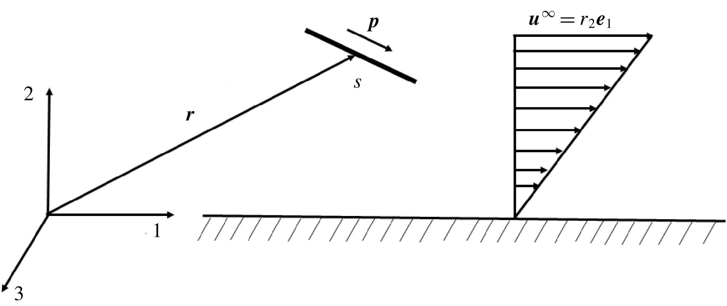
the coordinate in the vorticity direction of the imposed flow. This coordinate system is illustrated in figure 1. As illustrated,
 $s$
is the coordinate along the axis of the fibre. If
 $\boldsymbol{p}$
is the unit vector along the axis of the fibre with centre at
 $\boldsymbol{r}^{c}$
then any point on the fibre,
 $\boldsymbol{r}^{f}$
, is given as
 $\boldsymbol{r}^{f}=\boldsymbol{r}^{c}+\boldsymbol{p}s$
.
Sketch of fibre motion in the flow-gradient plane of the imposed shear flow inner region close to a wall. Direction ‘1’ is along the direction of the flow, ‘2’ is the velocity gradient direction which is normal to the wall and ‘3’ is along the vorticity of the imposed flow. The fibre is oriented along the unit vector
 $\boldsymbol{p}$
, with
 $s$
being the coordinate along the fibre.

The fibre experiences no net force
 $\boldsymbol{F}=\int \text{d}A\,\boldsymbol{n}\boldsymbol{\cdot }\unicode[STIX]{x1D748}=0$
and no net torque
 $\boldsymbol{L}=\int \text{d}A\,\boldsymbol{r}\times (\boldsymbol{n}\boldsymbol{\cdot }\unicode[STIX]{x1D748})=0$
, with
 $\boldsymbol{n}$
being the outward normal from the area
 $A$
into the fluid volume
 $V$
, and the fluid velocity is zero on the wall. Stokes flow reversibility implies that a fibre should not experience any net drift perpendicular to the wall at zero Reynolds number. Consistent with this expectation, Yang & Leal (Reference Yang and Leal1984) computed a time-oscillatory fibre translation in the 2-direction with no net drift as the fibres rotated in a periodic motion that approximated Jeffery orbits (Jeffery Reference Jeffery1922). A net drift away from the wall is expected at finite
 $Re$
along with the persistence of this oscillatory behaviour.
To obtain the lift velocity of the fibre at small Reynolds number in the case where the fibre lies within the viscous-dominated inner region near the wall,
 $h^{\ast }\ll L_{0}$
, we can expand the fluid velocity, pressure and fibre velocity in regular perturbation expansions in the small parameter
 $Re$
of the form
 $\boldsymbol{u}=\boldsymbol{u}^{0}+Re\,\boldsymbol{u}^{1}$
,
 $p=p^{0}+Re\,p^{1}$
and
 $\boldsymbol{v}=\boldsymbol{v}^{0}+Re\,\boldsymbol{v}^{1}$
, respectively. The lift velocity can then be obtained by averaging
 $Re\,\boldsymbol{v}^{1}$
over the Jeffery period of rotation of the fibre. The derivation of the perturbed fluid velocity
 $\boldsymbol{u}^{1}$
would be difficult. However, we can use a generalized reciprocal theorem to express the fibre velocity
 $\boldsymbol{v}^{1}$
in terms of a volume integral involving the Stokes flow field
 $\boldsymbol{u}^{0}$
for the shear flow problem and a comparison flow field
 $\boldsymbol{u}^{\prime }$
driven by a fibre translating in the 2-direction. In the following discussion, we first present the generalized reciprocal theorem. Next the Stokes flow field and comparison field are expressed using slender-body theory and hydrodynamic images with the wall. After that we discuss the averaging of the lift velocity over the Jeffery period of rotation to obtain a time-averaged result. To complete the analysis we will evaluate the finite
 $Re$
perturbations to the Jeffery orbit. This and other details of the time-averaged lift velocity calculation will be discussed in depth.
The generalized reciprocal theorem for a problem with weak fluid inertia (see Lovalenti & Brady Reference Lovalenti and Brady1993) can be obtained by considering the volume integral
 $$\begin{eqnarray}\displaystyle \int \unicode[STIX]{x1D735}\boldsymbol{\cdot }[\unicode[STIX]{x1D748}^{1}\boldsymbol{\cdot }\boldsymbol{u}^{\prime }-\unicode[STIX]{x1D748}^{\prime }\boldsymbol{\cdot }\boldsymbol{u}^{1}]\,\text{d}V, & & \displaystyle\end{eqnarray}$$
where
 $\boldsymbol{u}^{\prime }$
and
 $\unicode[STIX]{x1D748}^{\prime }$
are the fluid velocity and stress field for a Stokes flow comparison problem that satisfies
 $$\begin{eqnarray}\displaystyle \unicode[STIX]{x1D735}\boldsymbol{\cdot }\unicode[STIX]{x1D748}^{\prime }=0 & & \displaystyle\end{eqnarray}$$
and
 $$\begin{eqnarray}\displaystyle \unicode[STIX]{x1D735}\boldsymbol{\cdot }\boldsymbol{u}^{\prime }=0, & & \displaystyle\end{eqnarray}$$
along with boundary conditions
 $\boldsymbol{n}\boldsymbol{\cdot }\unicode[STIX]{x1D748}^{\prime }=(1/A_{f})\boldsymbol{e}_{2}$
on the fibre and
 $\boldsymbol{u}^{\prime }=0$
on the walls and at large distances from the fibre. Here
 $A_{f}$
is the surface area of the fibre.
Using the divergence theorem, one can obtain
 $$\begin{eqnarray}\displaystyle \int \unicode[STIX]{x1D735}\boldsymbol{\cdot }[\unicode[STIX]{x1D748}^{1}\boldsymbol{\cdot }\boldsymbol{u}^{\prime }-\unicode[STIX]{x1D748}^{\prime }\boldsymbol{\cdot }\boldsymbol{u}^{1}]\,\text{d}V & = & \displaystyle \int _{fibre}\text{d}A\,\boldsymbol{n}\boldsymbol{\cdot }[\unicode[STIX]{x1D748}^{\prime }\boldsymbol{\cdot }\boldsymbol{u}^{1}-\unicode[STIX]{x1D748}^{1}\boldsymbol{\cdot }\boldsymbol{u}^{\prime }]\nonumber\\ \displaystyle & & \displaystyle +\,\int _{wall}\text{d}A\,\boldsymbol{n}\boldsymbol{\cdot }[\unicode[STIX]{x1D748}^{\prime }\boldsymbol{\cdot }\boldsymbol{u}^{1}-\unicode[STIX]{x1D748}^{1}\boldsymbol{\cdot }\boldsymbol{u}^{\prime }]\nonumber\\ \displaystyle & & \displaystyle +\,\int _{\infty }\text{d}A\,\boldsymbol{n}\boldsymbol{\cdot }[\unicode[STIX]{x1D748}^{\prime }\boldsymbol{\cdot }\boldsymbol{u}^{1}-\unicode[STIX]{x1D748}^{1}\boldsymbol{\cdot }\boldsymbol{u}^{\prime }].\end{eqnarray}$$
The no-slip boundary condition implies that the integral on the wall vanishes. The fluid velocity disturbance due to the fibre decays as
 $1/r^{2}$
in both the shear and comparison problem so the integral on the bounding surface vanishes as its distance goes to infinity. Finally, the rigid-body motion, no-force and no-torque conditions on the fibre in shear flow along with the specified force density on the fibre (
 $\int \text{d}A\,\boldsymbol{n}\boldsymbol{\cdot }\unicode[STIX]{x1D748}^{\prime }=\boldsymbol{e}_{2}$
) in the comparison problem simplify the surface integral on the fibre to yield
 $$\begin{eqnarray}\displaystyle \int \unicode[STIX]{x1D735}\boldsymbol{\cdot }[\unicode[STIX]{x1D748}^{1}\boldsymbol{\cdot }\boldsymbol{u}^{\prime }-\unicode[STIX]{x1D748}^{\prime }\boldsymbol{\cdot }\boldsymbol{u}^{1}]\,\text{d}V=\boldsymbol{v}^{1}\boldsymbol{\cdot }\boldsymbol{e}_{2}. & & \displaystyle\end{eqnarray}$$
The equations of motion for the shear flow and comparison problem yield
 $$\begin{eqnarray}\displaystyle \int \unicode[STIX]{x1D735}\boldsymbol{\cdot }[\unicode[STIX]{x1D748}^{1}\boldsymbol{\cdot }\boldsymbol{u}^{\prime }-\unicode[STIX]{x1D748}^{\prime }\boldsymbol{\cdot }\boldsymbol{u}^{1}]\,\text{d}V=Re\int \left[\frac{\unicode[STIX]{x2202}\boldsymbol{u}^{0}}{\unicode[STIX]{x2202}t}+\boldsymbol{u}^{0}\boldsymbol{\cdot }\unicode[STIX]{x1D735}\boldsymbol{u}^{0}\right]\boldsymbol{\cdot }\boldsymbol{u}^{\prime }\,\text{d}V. & & \displaystyle\end{eqnarray}$$
Combining (2.6) and (2.7), we obtain an expression for the inertia-induced translational velocity of the fibre perpendicular to the wall in terms of the Stokes flow shear and comparison fluid velocity fields
 $$\begin{eqnarray}\displaystyle \boldsymbol{v}^{1}\boldsymbol{\cdot }\boldsymbol{e}_{2}=Re\int \left[\frac{\unicode[STIX]{x2202}\boldsymbol{u}^{0}}{\unicode[STIX]{x2202}t}+\boldsymbol{u}^{0}\boldsymbol{\cdot }\unicode[STIX]{x1D735}\boldsymbol{u}^{0}\right]\boldsymbol{\cdot }\boldsymbol{u}^{\prime }\,\text{d}V. & & \displaystyle\end{eqnarray}$$
The Stokes flow field
 $\boldsymbol{u}^{0}$
consists of the imposed flow (
 $\boldsymbol{u}^{\infty }$
) and the disturbance field (
 $\boldsymbol{u}^{D}$
), created by the presence of the fibre and the no-slip wall. This disturbance velocity field can be captured by a collection of singularities along with the driving force behind it. The driving force experienced by the fibre in quiescent flow is qualitatively and quantitatively different from when it is placed in a shear flow. However, the system of singularities remains the same in both cases.
A thin fibre in low-
 $Re$
flow can effectively be replaced by a collection of Stokeslets, the fundamental singularities in a Stokes flow. A Stokeslet near a no-slip wall was studied by Blake & Chwang (Reference Blake and Chwang1974). They found that a no-slip wall at
 $(r_{1},r_{2}=0,r_{3})$
, in the presence of a Stokeslet placed at
 $\boldsymbol{r}^{f}$
, can be replaced by another Stokeslet as well as a force dipole and a potential dipole placed at
 $\boldsymbol{r}^{im}=(r_{1}^{f},-r_{2}^{f},r_{3}^{f})$
. These singularities are mathematically represented by a Green’s function. The overall non-dimensional Green’s function of the fibre and no-slip wall system causing disturbance to the fluid velocity at
 $\boldsymbol{r}$
is given by
 $$\begin{eqnarray}\displaystyle \unicode[STIX]{x1D642}(\boldsymbol{r},s)=\unicode[STIX]{x1D642}^{S}(\overline{\boldsymbol{r}})-\unicode[STIX]{x1D642}^{S}(\overline{\boldsymbol{r}}^{im})-2(r_{2}^{f})\unicode[STIX]{x1D642}^{FD}(\overline{\boldsymbol{r}}^{im})+2(r_{2}^{f})^{2}\unicode[STIX]{x1D642}^{PD}(\overline{\boldsymbol{r}}^{im}). & & \displaystyle\end{eqnarray}$$
Here,
 $\overline{\boldsymbol{r}}=\boldsymbol{r}-\boldsymbol{r}^{f}$
,
 $\overline{\boldsymbol{r}}^{im}=\boldsymbol{r}^{im}-\boldsymbol{r}^{f}$
,
 $\unicode[STIX]{x1D642}^{S}$
is the Stokeslet,
 $\unicode[STIX]{x1D642}^{FD}$
is the force dipole and
 $\unicode[STIX]{x1D642}^{PD}$
is the potential dipole. The individual functions, non-dimensionalized by
 $\unicode[STIX]{x1D707}$
, are given as
 $$\begin{eqnarray}\displaystyle & \displaystyle \unicode[STIX]{x1D60E}_{ij}^{S}(\boldsymbol{r})=\frac{1}{8\unicode[STIX]{x03C0}r}\left[\unicode[STIX]{x1D6FF}_{ij}+\frac{r_{i}r_{j}}{r^{2}}\right], & \displaystyle\end{eqnarray}$$
 $$\begin{eqnarray}\displaystyle & \displaystyle \unicode[STIX]{x1D60E}_{ij}^{FD}(\boldsymbol{r})=\frac{1}{8\unicode[STIX]{x03C0}}\left[r_{2}\unicode[STIX]{x1D60E}_{ij}^{PD}(\boldsymbol{r})\pm \frac{\unicode[STIX]{x1D6FF}_{j2}r_{i}-\unicode[STIX]{x1D6FF}_{i2}r_{j}}{r^{3}}\right], & \displaystyle\end{eqnarray}$$
 $$\begin{eqnarray}\displaystyle & \displaystyle \unicode[STIX]{x1D60E}_{ij}^{PD}(\boldsymbol{r})=\pm \frac{1}{8\unicode[STIX]{x03C0}r^{3}}\left[\unicode[STIX]{x1D6FF}_{ij}-3\frac{r_{i}r_{j}}{r^{2}}\right]. & \displaystyle\end{eqnarray}$$
In (2.11) and (2.12) there is a plus sign for
 $j=1$
and 3 and a minus sign for
 $j=2$
. Thus it is possible to obtain
 $\boldsymbol{u}^{D}$
at any fluid location
 $\boldsymbol{r}$
through an integral in
 $s$
, spanning the whole length of the fibre, as
 $$\begin{eqnarray}\displaystyle u_{i}^{D}(\boldsymbol{r})=\int _{-1}^{1}\text{d}s\,f_{j}(s)\,\unicode[STIX]{x1D60E}_{ji}(\boldsymbol{r},s), & & \displaystyle\end{eqnarray}$$
where
 $\boldsymbol{f}(s)$
is the force distribution on the fibre.
To evaluate
 $\boldsymbol{u}^{D}$
the force per unit length
 $\boldsymbol{f}(s)$
needs to be determined. From slender-body theory (see Batchelor Reference Batchelor1970), the governing equation for
 $\boldsymbol{f}(s)$
is given as
 $$\begin{eqnarray}\displaystyle v_{i}^{0}+\unicode[STIX]{x1D716}_{ijk}\unicode[STIX]{x1D6FA}_{j}\,p_{k}s & = & \displaystyle w_{i}(\boldsymbol{r}^{c}+\boldsymbol{p}\,s)+\frac{f_{j}}{4\unicode[STIX]{x03C0}}[\unicode[STIX]{x1D6FF}_{ij}+p_{i}p_{j}]\left[\ln 2\unicode[STIX]{x1D705}+\ln \left[\frac{[1-s^{2}]^{1/2}}{a(s)}\right]\right]\qquad \nonumber\\ \displaystyle & & \displaystyle +\,\frac{f_{j}}{8\unicode[STIX]{x03C0}}[\unicode[STIX]{x1D6FF}_{ij}-3p_{i}p_{j}]+\frac{f_{j}}{8\unicode[STIX]{x03C0}}[\unicode[STIX]{x1D6FF}_{ij}+p_{i}p_{j}]\int _{-1}^{1}\frac{f_{j}(s^{\prime })-f_{j}(s)}{|s-s^{\prime }|}\,\text{d}s^{\prime },\qquad\end{eqnarray}$$
where
 $\boldsymbol{v}^{0}$
and
 $\unicode[STIX]{x1D734}$
are the fibre centre of mass translational and rotational velocities at zero
 $Re$
,
 $a(s)$
is the radius of the fibre at any given location on the fibre normalized with the characteristic radius (
 $a(s)=1$
for a cylindrical fibre),
 $\unicode[STIX]{x1D705}=l/a$
is the aspect ratio and
 $\boldsymbol{w}$
is the far-field velocity consisting of the imposed shear flow and image velocity. In solving (2.14) we assume the fibre has a large aspect ratio and expand in terms of the small parameter
 $\unicode[STIX]{x1D716}=1/(\ln 2\unicode[STIX]{x1D705})$
. This leads to a perturbation in
 $\unicode[STIX]{x1D716}$
for
 $\boldsymbol{f}$
as well as
 $\boldsymbol{v}^{0},\boldsymbol{w},\boldsymbol{u}^{D}$
and
 $\dot{\boldsymbol{p}}$
. These can be expressed as
 $$\begin{eqnarray}\displaystyle \left.\begin{array}{@{}c@{}}\displaystyle \boldsymbol{f}=\unicode[STIX]{x1D716}\boldsymbol{f}_{1}+\unicode[STIX]{x1D716}^{2}\boldsymbol{f}_{2}+\cdots \,,\\ \displaystyle \dot{\boldsymbol{p}}=\dot{\boldsymbol{p}}_{0}+\unicode[STIX]{x1D716}\dot{\boldsymbol{p}}_{1}+\cdots \,,\\ \displaystyle \boldsymbol{v}^{0}=\boldsymbol{v}_{0}^{0}+\unicode[STIX]{x1D716}\boldsymbol{v}_{1}^{0}+\cdots \,,\\ \displaystyle \boldsymbol{w}=\boldsymbol{w}_{0}+\unicode[STIX]{x1D716}\boldsymbol{w}_{1}+\cdots \,,\\ \displaystyle \boldsymbol{u}^{D}=\unicode[STIX]{x1D716}\boldsymbol{u}_{1}^{D}+\unicode[STIX]{x1D716}^{2}\boldsymbol{u}_{2}^{D}+\cdots \,.\end{array}\right\} & & \displaystyle\end{eqnarray}$$
The subscripts here denote the order of the term with respect to the expansion in
 $\unicode[STIX]{x1D716}$
. In this study we compute the lift velocity to
 $O(\unicode[STIX]{x1D716}^{2})$
by retaining the terms indicated in (2.15) for the force per unit length, fibre rotation and translation rate, far-field velocity and fluid velocity disturbance.
To obtain
 $\boldsymbol{u}_{1}^{D}$
, the leading-order disturbance velocity field in the
 $\unicode[STIX]{x1D716}$
expansion, we evaluate
 $\boldsymbol{f}_{1}$
. The force distribution on the fibre at
 $O(\unicode[STIX]{x1D716})$
is given as
 $$\begin{eqnarray}\displaystyle \frac{1}{4\unicode[STIX]{x03C0}}f_{1,i}[\unicode[STIX]{x1D6FF}_{ij}+p_{i}p_{j}]=v_{i}^{0}+\unicode[STIX]{x1D716}_{ijk}\unicode[STIX]{x1D6FA}_{j}p_{k}s & - & \displaystyle w_{0,i}(\boldsymbol{r}^{c}+\boldsymbol{p}\,s).\end{eqnarray}$$
At leading order in
 $\unicode[STIX]{x1D716}$
, the far-field velocity
 $\boldsymbol{w}_{0}$
is the imposed shear flow
 $\boldsymbol{u}^{\infty }$
. In a simple shear flow the dynamics of the fibre motion at finite
 $Re$
was studied by Subramanian & Koch (Reference Subramanian and Koch2005). They showed that inertia forces the fibre towards motion in the flow-gradient plane. This constraint simplifies (2.16) to
 $$\begin{eqnarray}\displaystyle \boldsymbol{f}_{1}=4\unicode[STIX]{x03C0}\,\boldsymbol{p}\,s\cos \unicode[STIX]{x1D719}\sin \unicode[STIX]{x1D719}. & & \displaystyle\end{eqnarray}$$
Here
 $\unicode[STIX]{x1D719}$
is the dihedral angle between the flow-vorticity and the fibre-vorticity planes.
To obtain
 $\boldsymbol{u}_{2}^{D}$
we require the force distribution at
 $O(\unicode[STIX]{x1D716}^{2})$
, which is
 $$\begin{eqnarray}\displaystyle f_{2,j}=\unicode[STIX]{x03C0}p_{i}\sin 2\unicode[STIX]{x1D719}[2s\ln [1-s^{2}]-3s]-4\unicode[STIX]{x03C0}\left[\unicode[STIX]{x1D6FF}_{ij}-\frac{p_{i}p_{j}}{2}\right] & w_{1,i}(\boldsymbol{r}^{c}+\boldsymbol{p}\,s). & \displaystyle\end{eqnarray}$$
To evaluate
 $\boldsymbol{w}_{1}$
we use the disturbance velocity result from (2.13) and evaluate only the image component. This is given as
 $$\begin{eqnarray}\displaystyle \boldsymbol{w}_{1}(\boldsymbol{r})=\int _{-1}^{1}\text{d}s\,f_{1,j}(s)\,\unicode[STIX]{x1D60E}_{ji}^{I}(\boldsymbol{r},s). & & \displaystyle\end{eqnarray}$$
Here
 $\unicode[STIX]{x1D60E}_{ji}^{I}(\boldsymbol{r},s)$
is due to the image system that captures wall reflection. This is given as
 $$\begin{eqnarray}\displaystyle \unicode[STIX]{x1D642}^{I}(\boldsymbol{r},s)=-\unicode[STIX]{x1D642}^{S}(\overline{\boldsymbol{r}}^{im})-2(r_{2}^{f})\unicode[STIX]{x1D642}^{FD}(\overline{\boldsymbol{r}}^{im})+2(r_{2}^{f})^{2}\unicode[STIX]{x1D642}^{PD}(\overline{\boldsymbol{r}}^{im}). & & \displaystyle\end{eqnarray}$$
With a complete description of
 $\unicode[STIX]{x1D642}(\boldsymbol{r},s)$
and
 $\boldsymbol{f}(s)$
known at the first two orders in
 $\unicode[STIX]{x1D716}$
, equation (2.13) can be evaluated to find
 $\boldsymbol{u}^{D}$
and by extension
 $\boldsymbol{u}^{0}$
. To evaluate (2.8) and obtain the lift velocity, information on
 $\boldsymbol{u}^{\prime }$
is also needed. In the quiescent comparison flow the disturbance velocity field is calculated using (2.13) with a specified force distribution
 $\int \boldsymbol{f}^{\prime }(s)\,\text{d}s=\int \text{d}A\boldsymbol{n}\boldsymbol{\cdot }\unicode[STIX]{x1D748}^{\prime }=\boldsymbol{e}_{2}$
.
The fibre rotates in a shear flow and samples all possible orientations in the flow-gradient plane. Orientation plays an important role in determining
 $\boldsymbol{f}(s)$
, as evident by the strong dependence on
 $\unicode[STIX]{x1D719}$
in (2.17) and (2.18). The temporal evolution of fibres in Stokes flow was studied by Yang & Leal (Reference Yang and Leal1984) who found that, at zero
 $Re$
, they undergo periodic flipping motion. This periodic motion is expected to persist at small, but finite,
 $Re$
. At zero
 $Re$
, Jeffery (Reference Jeffery1922) studied the periodic orbits of ellipsoidal particles in an unbounded simple shear flow. Jeffery’s calculation properly captures the flipping motion of fibres near a wall, as shown in experimental studies carried out by Stover & Cohen (Reference Stover and Cohen1990) and Moses, Advani & Reinhardt (Reference Moses, Advani and Reinhardt2001). In this study we will assume that these periodic orbits (commonly referred to as Jeffery orbits) describe the temporal dynamics of the fibre at finite
 $Re$
near a wall.
During the flipping motion of a fibre near a wall its centre of mass executes oscillatory motion in the 2-direction in Stokes flow. The fibre translates away from and towards the wall in the compressional and extensional quadrants, respectively (Yang & Leal Reference Yang and Leal1984). The symmetry of this oscillatory motion is broken by fluid inertia leading to a net drift away from the wall. The symmetry breaking occurs in two ways. First, the inertial correction to the fluid velocity induces a net positive velocity in the 2-direction. Second, inertial effects change the rotation rate of the fibre causing it to spend more time in the compressional quadrant than the extensional quadrant, so that the viscous forces lead to a net drift away from the wall.
The finite inertia correction to the evolution of the orientation dynamics of a fibre was studied by Subramanian & Koch (Reference Subramanian and Koch2005). For dynamics in the flow-gradient plane, this is given as
 $$\begin{eqnarray}\displaystyle \dot{\unicode[STIX]{x1D719}} & = & \displaystyle \frac{-1}{\unicode[STIX]{x1D705}^{2}+1}[\unicode[STIX]{x1D705}^{2}\sin ^{2}\unicode[STIX]{x1D719}+\cos ^{2}\unicode[STIX]{x1D719}]\nonumber\\ \displaystyle & & \displaystyle -\,\frac{Re}{\ln \,\unicode[STIX]{x1D705}}\sin \unicode[STIX]{x1D719}\cos \unicode[STIX]{x1D719}\left[\frac{1}{6}\sin ^{2}\unicode[STIX]{x1D719}-\frac{1}{15}\cos ^{2}\unicode[STIX]{x1D719}\right].\end{eqnarray}$$
Equation (2.21) includes a correction of a typographical error in the original paper that was first noted in Shin et al. (Reference Shin, Koch and Subramanian2009).
The time period
 $T$
for one revolution in a Jeffery orbit is given as
 $$\begin{eqnarray}\displaystyle T=2\unicode[STIX]{x03C0}\left[\unicode[STIX]{x1D705}+\frac{1}{\unicode[STIX]{x1D705}}\right]. & & \displaystyle\end{eqnarray}$$
The finite inertia correction to the time period is
 $O(Re^{3/2})$
for fibres much smaller than the Oseen length (see Marath & Subramanian Reference Marath and Subramanian2017). Thus, it does not influence the lift velocity at leading order in
 $Re$
.
Due to the rapid variation of drift over a Jeffery orbit it is of interest to obtain a time-averaged result
 $\int \text{d}t\,\boldsymbol{v}\boldsymbol{\cdot }\boldsymbol{e}_{2}/T$
. For ease of analysis it can be transformed into
 $\unicode[STIX]{x1D719}$
coordinates using (2.21). This is given as
 $$\begin{eqnarray}\displaystyle v_{l} & = & \displaystyle \frac{Re}{T}\int _{0}^{2\unicode[STIX]{x03C0}}\,\text{d}\unicode[STIX]{x1D719}\,\int \text{d}V\left[\frac{\unicode[STIX]{x2202}\boldsymbol{u}^{0}}{\unicode[STIX]{x2202}t}+\boldsymbol{u}^{0}\boldsymbol{\cdot }\unicode[STIX]{x1D735}\boldsymbol{u}^{0}\right]\boldsymbol{\cdot }\boldsymbol{u}^{\prime }\frac{1}{\dot{\unicode[STIX]{x1D719}}^{0}}\nonumber\\ \displaystyle & & \displaystyle +\,\frac{Re}{T}\int _{0}^{2\unicode[STIX]{x03C0}}\text{d}\unicode[STIX]{x1D719}\,\boldsymbol{v}^{0}\boldsymbol{\cdot }\boldsymbol{e}_{2}\left(\frac{-\dot{\unicode[STIX]{x1D719}}^{1}}{(\dot{\unicode[STIX]{x1D719}}^{0})^{2}}\right).\end{eqnarray}$$
The orientation evolution has been expanded based on a regular perturbation in
 $Re$
that is given as
 $\dot{\unicode[STIX]{x1D719}}=\dot{\unicode[STIX]{x1D719}}^{0}+Re\,\dot{\unicode[STIX]{x1D719}}^{1}+\cdots \,$
and the second term in (2.23) was obtained through a binomial expansion. The first term on the right-hand side was obtained using (2.8). A regular perturbation in
 $\unicode[STIX]{x1D716}$
similar to those expressed in (2.15) can be extended to this time-averaged lift velocity and is given as
 $$\begin{eqnarray}\displaystyle v_{l}=\unicode[STIX]{x1D716}v_{l1}+\unicode[STIX]{x1D716}^{2}v_{l2}+\cdots \,. & & \displaystyle\end{eqnarray}$$
It is evident that
 $v_{l0}=0$
due to the nature of the force distribution. We will evaluate the first two non-zero terms
 $v_{l1}$
and
 $v_{l2}$
in this study.
Owing to the quasi-steady nature of Stokes flow the partial time derivative of the fluid velocity appearing in (2.23) can be related to the time variation of the fibre orientation and centre of mass position:
 $$\begin{eqnarray}\displaystyle \frac{\unicode[STIX]{x2202}\boldsymbol{u}^{0}}{\unicode[STIX]{x2202}t}=\frac{\unicode[STIX]{x2202}\boldsymbol{u}^{0}}{\unicode[STIX]{x2202}\unicode[STIX]{x1D719}}\dot{\unicode[STIX]{x1D719}}^{0}+\frac{\unicode[STIX]{x2202}\boldsymbol{r}^{c}}{\unicode[STIX]{x2202}t}\boldsymbol{\cdot }\unicode[STIX]{x1D735}\boldsymbol{u}^{0}. & & \displaystyle\end{eqnarray}$$
While computing the
 $O(\unicode[STIX]{x1D716})$
lift velocity, the time dependence of
 $\boldsymbol{r}^{c}$
can be removed by adopting a reference frame translating with the
 $O(1)$
particle translational velocity and
 $\unicode[STIX]{x2202}\unicode[STIX]{x1D719}/\unicode[STIX]{x2202}t$
can be evaluated using the Jeffery orientation evolution in (2.21). At
 $O(\unicode[STIX]{x1D716}^{2})$
there are additional contributions to the time derivatives of the fibre orientation and position caused by the
 $O(\unicode[STIX]{x1D716})$
wall reflection fluid velocity disturbance. These are given as
 $$\begin{eqnarray}\displaystyle \left.\begin{array}{@{}c@{}}\displaystyle {\dot{p}}_{1,i}={\textstyle \frac{3}{2}}\int _{-1}^{1}\text{d}s\,[\unicode[STIX]{x1D6FF}_{ij}-p_{0,i}p_{0,j}]w_{1,j}(\boldsymbol{r}^{c}+\boldsymbol{p}\,s)s,\\ \displaystyle \boldsymbol{v}_{1}^{0}={\textstyle \frac{1}{2}}\int _{-1}^{1}\text{d}s\,\boldsymbol{w}_{1}(\boldsymbol{r}^{c}+\boldsymbol{p}s),\end{array}\right\} & & \displaystyle\end{eqnarray}$$
where
 $\boldsymbol{w}_{1}$
is given in (2.19).
Here
 $\boldsymbol{v}_{0}^{0}\boldsymbol{\cdot }\boldsymbol{e}_{2}=0$
so the non-zero contribution to the second term on the right-hand side of (2.23) involves
 $\boldsymbol{v}_{1}^{0}$
, which is
 $O(\unicode[STIX]{x1D716})$
. The finite
 $Re$
correction to the orientation dynamics is also
 $O(\unicode[STIX]{x1D716})$
. Thus, the leading contribution to lift velocity due to finite
 $Re$
perturbations of the rotational dynamics appears in
 $v_{l2}$
.
The lift velocity calculation involves nested integrals spanning a large domain. The spatial coordinate
 $r_{i}$
spans
 $-\infty$
to
 $\infty$
when
 $i=1,3$
and
 $0$
to
 $\infty$
for
 $i=2$
, thus capturing all of the fluid volume. Based on symmetry, the angular integration in
 $\unicode[STIX]{x1D719}$
from 0 to
 $2\unicode[STIX]{x03C0}$
can be related to four times the integral from
 $0$
to
 $\unicode[STIX]{x03C0}/2$
. The disturbance velocity field driving the lift velocity involves an integral over
 $s$
, thus capturing the net effect of the singularities of the fibre and its images. The higher-order (in
 $\unicode[STIX]{x1D716}$
) force distribution as well as unsteadiness (see (2.26)) depends on the image velocity, which in turn requires integration over
 $s$
for the image singularities. All of these nested integrals are numerically evaluated using an adaptive quadrature scheme. For this purpose a combination of the ‘integral’ and ‘integral2’ routines available in MATLAB is used.
The dimensional lift velocity (
 $v_{l}^{\ast }$
) of a fibre will be proportional to the characteristic shear velocity
 $\dot{\unicode[STIX]{x1D6FE}}l$
based on the chosen non-dimensionalization. However, it is modified by three factors: fluid inertia, flipping motion in a Jeffery orbit and the thinness of the fibre. In the absence of fluid inertia, i.e Stokes flow, there is no net migration. At small but finite Reynolds number, the lift velocity is proportional to
 $Re$
. In a Jeffery orbit the time period is
 $O(\unicode[STIX]{x1D705})$
whereas the flipping motion, during which significant migration away from the wall occurs, takes place over
 $O(1)$
time. Thus a factor of
 $\unicode[STIX]{x1D705}^{-1}$
appears in the time-averaged lift velocity. Finally, the disturbance velocity field, which drives the migration away from the wall, is shaped by the geometry of the fibre. For a high-aspect-ratio fibre this is characterized by
 $\unicode[STIX]{x1D716}$
. Thus, the scaling of the lift velocity can be given as
 $\unicode[STIX]{x1D70C}\dot{\unicode[STIX]{x1D6FE}}^{2}l^{2}a/(\unicode[STIX]{x1D707}\ln [2l/a])$
when not making contact with the wall.
In contrast to a fibre, the hydrodynamic lift on a sphere, while also being a finite
 $Re$
effect, has none of the complexities associated with orientation and aspect ratio. Thus, the dimensional lift velocity of a sphere scales as
 $\unicode[STIX]{x1D70C}\dot{\unicode[STIX]{x1D6FE}}^{2}a^{3}/\unicode[STIX]{x1D707}$
, where
 $a$
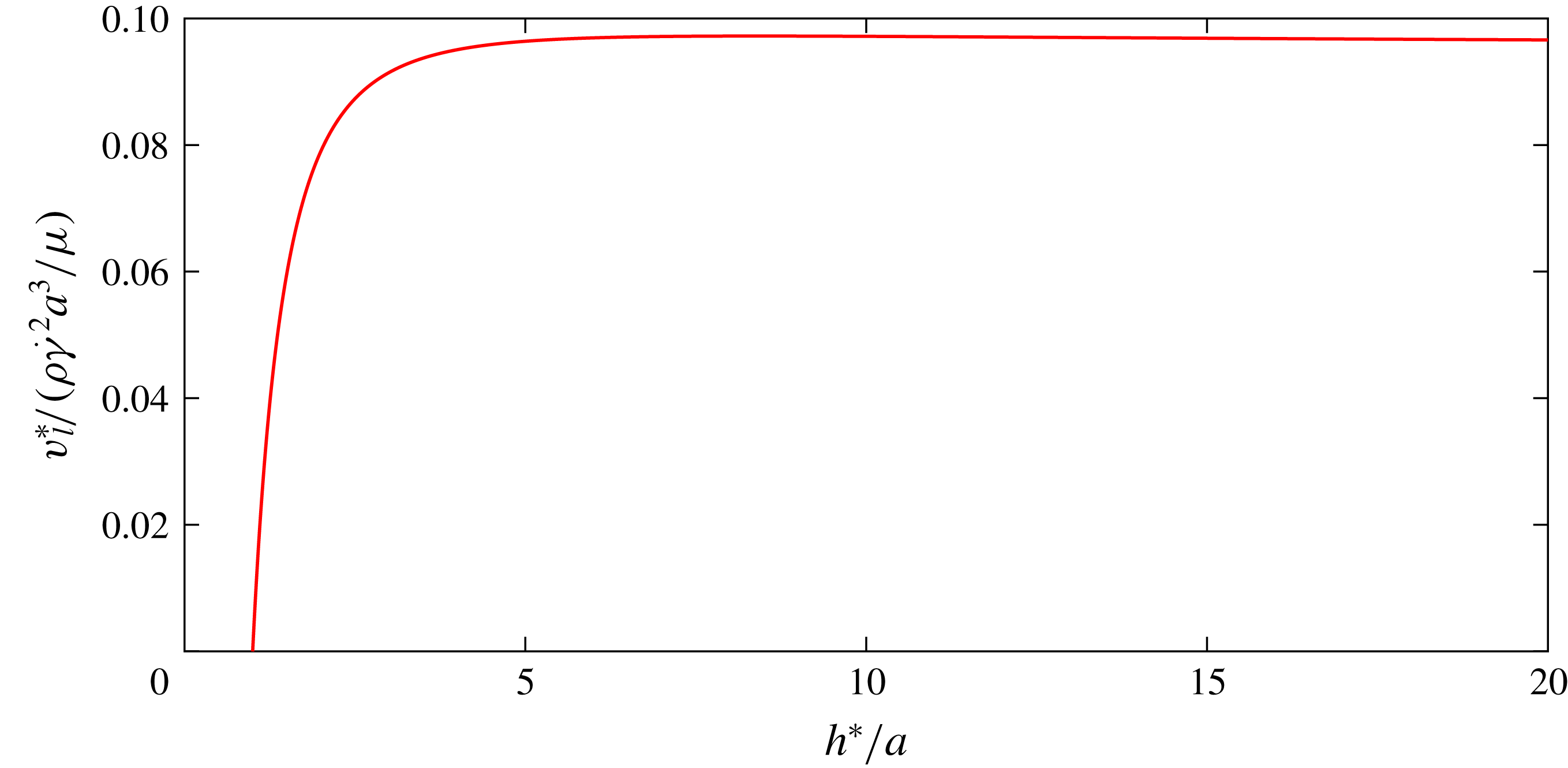
is the characteristic length of the sphere which is its radius. Figure 2 gives the variation of the lift velocity of a sphere with distance from the wall in the inner region. The lift velocity is scaled as
 $\unicode[STIX]{x1D70C}\dot{\unicode[STIX]{x1D6FE}}^{2}a^{3}/\unicode[STIX]{x1D707}$
in this plot. This result is obtained using the lift force derived by Cherukat & McLaughlin (Reference Cherukat and McLaughlin1994) for the special case of no force along the streamline, along with the appropriate Stokes resistance function (see Brenner Reference Brenner1961; Cox & Brenner Reference Cox and Brenner1967). The lift force does not go to zero as the sphere approaches the wall but the Stokes resistance function, due to lubrication effects, diverges leading to a decay of the lift velocity of the sphere to zero. Conversely the resistance decays away from the wall and so the lift velocity approaches a constant at separations that are large but still lie within the inner region.
Lift velocity for a sphere as a function of distance from the wall in the inner region. Parameter
 $h^{\ast }$
represents the dimensional distance of the sphere of radius
 $a$
from the wall. The lift velocity is obtained using the lift force calculation of Cherukat & McLaughlin (Reference Cherukat and McLaughlin1994) in conjunction with Stokes resistance functions (see Brenner Reference Brenner1961; Cox & Brenner Reference Cox and Brenner1967).

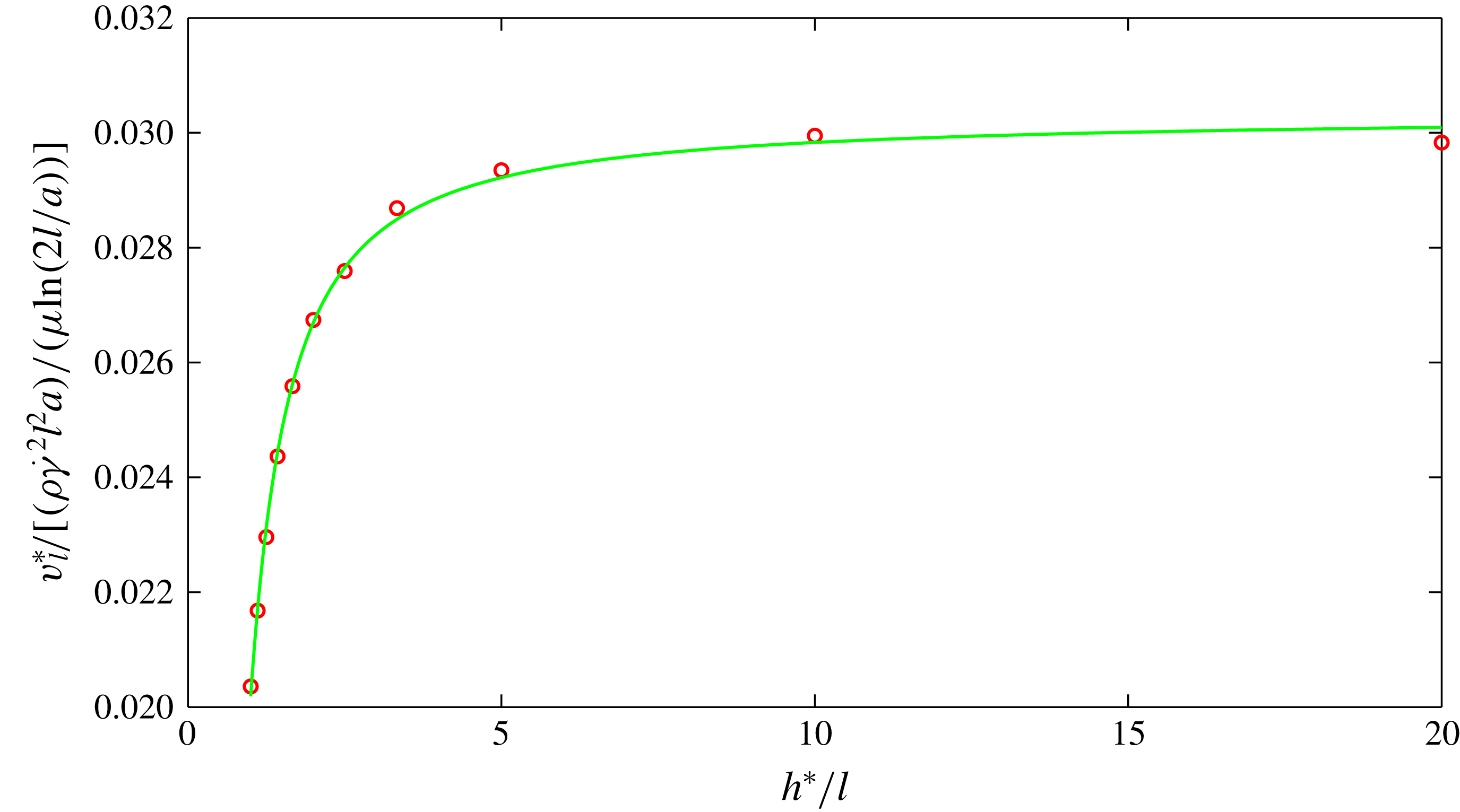
Figure 3 presents the computed lift velocity for the fibre at
 $O(\unicode[STIX]{x1D716}Re)$
. The lift velocity presented is scaled as
 $\unicode[STIX]{x1D70C}\dot{\unicode[STIX]{x1D6FE}}^{2}l^{2}a/(\unicode[STIX]{x1D707}\ln [2l/a])$
and given as a function of the non-dimensional distance of the centre of the fibre from the wall. When the fibre approaches the wall its lift velocity, unlike that of a sphere, does not tend to zero. This can be attributed to the finite Stokes resistance for the sharp edges of the fibre as pointed out by Harlen, Sundararajakumar & Koch (Reference Harlen, Sundararajakumar and Koch1999). These sharp ends can make contact with the wall in finite time. Additionally, the fibre end only contacts the wall at one instant in time during the fibre’s periodic motion when
 $h^{\ast }=l$
. As the distance from the wall increases the Stokes resistance experienced decreases and the lift velocity increases monotonically. At large distances from the wall, but still in the inner region, the lift velocity asymptotes at leading order to a value of
 $0.0303\unicode[STIX]{x1D70C}\dot{\unicode[STIX]{x1D6FE}}^{2}l^{2}a/(\unicode[STIX]{x1D707}\ln [2l/a])$
. Qualitatively, at
 $O(\unicode[STIX]{x1D716})$
, the lift velocity captures the breaking of the stress symmetry that leads to a net migration due to a simple interaction of the imposed shear flow with a thin geometry.
Variation of the
 $O(\unicode[STIX]{x1D716}Re)$
fibre lift velocity as a function of distance from the wall. Circles show the evaluated data and the line shows the fit given by
 $v_{l1}=-0.0057/h^{2}-0.0044/h+0.0303$
.

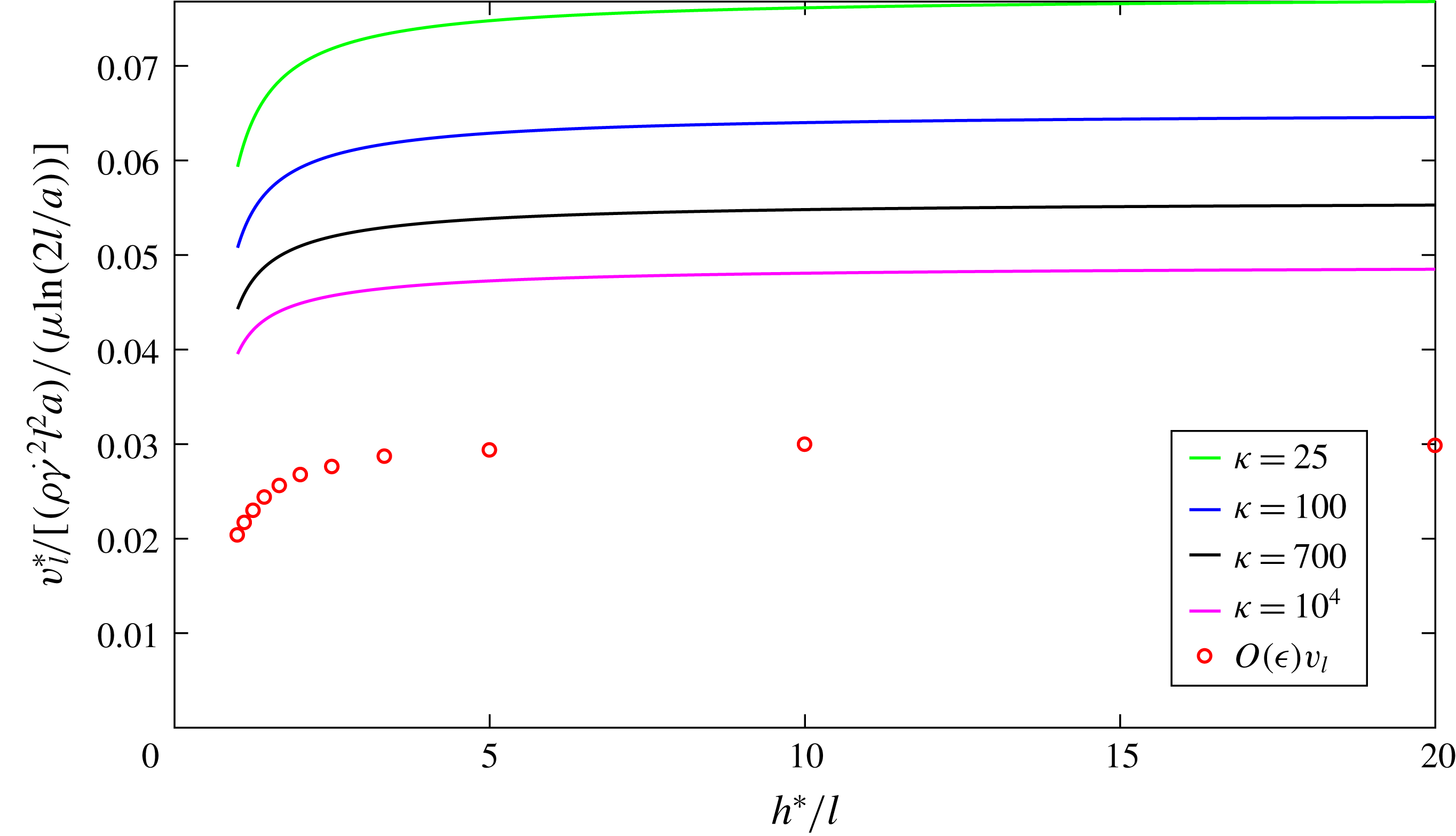
Variation of the
 $O(Re)$
lift velocity calculated based on the first two terms of the slender-body theory expansion for a fibre and expressed as a function of distance from the wall at various aspect ratios. The aspect ratios of the curves going from highest to lowest asymptote values are 25, 100, 700 and
 $10^{4}$
. Circles represent the lift velocity at
 $O(\unicode[STIX]{x1D716})$
.

Figure 4 shows the
 $O(Re)$
fibre lift velocity based on the first two terms of the slender-body theory expansion at various
 $\unicode[STIX]{x1D705}$
plotted as a function of the non-dimensional distance from the wall. Despite scaling the lift velocity with the leading-order scaling of
 $\unicode[STIX]{x1D70C}\dot{\unicode[STIX]{x1D6FE}}^{2}l^{2}a/(\unicode[STIX]{x1D707}\ln [2l/a])$
, there remains a significant dependence on the aspect ratio with the lift velocity reaching significantly higher values at smaller aspect ratio. Even at an aspect ratio as high as
 $10^{4}$
, the asymptotic value of the total lift velocity is about 50 % larger than the
 $O(\unicode[STIX]{x1D716})$
lift velocity. This indicates that a significant contribution to the lift velocity comes from the
 $O(\unicode[STIX]{x1D716}^{2})$
term. This higher-order term includes a number of qualitative features not present at
 $O(\unicode[STIX]{x1D716})$
including the influence of the wall reflection, the oscillatory translation of the fibre perpendicular to the wall, finite
 $Re$
perturbations of the periodic motion of the fibre and the effects of the precise variation of the fibre thickness as captured by the
 $\ln [(1-s^{2})^{1/2}/a(s)]$
term in (2.14). At
 $O(\unicode[STIX]{x1D716}^{3})$
and higher orders, no qualitatively new mechanisms come into play. Quantitatively the first two terms in slender-body theory are expected to dominate the lift velocity calculation. To test this we calculate, using the analysis of Batchelor (Reference Batchelor1970), the stresslet of a slender body and find that even for the lowest chosen
 $\unicode[STIX]{x1D705}$
, of 25, the
 $O(\unicode[STIX]{x1D716}^{3})$
term only changes the result by 6 %. We expect similar errors for the lift velocity when two terms of the slender-body theory are retained and
 $\unicode[STIX]{x1D705}$
of 25 is considered.
3 Lift velocity of a fibre experiencing wall contacts
When
 $h<1$
the dominant contribution to the lift velocity of a fibre in wall-bounded shear flow of small but finite inertia comes from the contact force due to solid-body interactions coupled with inertial rotation. For
 $h<1$
the orbit in the flow-gradient plane preferred based on inertial rotation is no longer accessible. Thus, the inertial torque driving the fibre towards the flow-gradient plane and the wall contact force compete to influence the fibre orientation. In this section, we will analyse the coupled action of these two mechanisms. First we will track the trajectory of the fibre for
 $h<1$
. Then we will develop an analytical model for the lift velocity in the
 $h<1$
regime by assuming the fibre follows a quasi-steady Jeffery orbit that just grazes the wall. Wall interactions are shaped by friction as well as normal forces. Thus, we consider the two limiting cases of a frictionless contact and a no-slip sticking solid-body contact. Our models for both these cases are validated against numerically computed trajectories.
A fibre in a simple shear flow adjacent to a wall is pushed away from it by the wall contact force. In addition, any fibre with an orientation out of the flow-gradient plane is pushed further out of the plane. This effect was experimentally observed by Stover & Cohen (Reference Stover and Cohen1990) and they referred to it as pole vaulting. A number of studies (see Jayageeth, Sharma & Singh Reference Jayageeth, Sharma and Singh2009; Ku & Lin Reference Ku and Lin2009; Scheuer et al.
Reference Scheuer, Abisset-Chavanne, Chinesta and Keunings2016; Nagel et al.
Reference Nagel, Brun, Berthet, Lindner, Gallaire and Duprat2018) have built on the work of Stover and Cohen and analysed the trajectory of wall-bounded fibres in Stokes flow. At finite
 $Re$
many studies have looked at dynamics of spheroids in an unbounded flow (see Khayat & Cox Reference Khayat and Cox1989; Subramanian & Koch Reference Subramanian and Koch2005; Einarsson et al.
Reference Einarsson, Candelier, Lundell, Angilella and Mehlig2015a
,Reference Einarsson, Candelier, Lundell, Angilella and Mehlig
b
; Dabade et al.
Reference Dabade, Marath and Subramanian2016; Marath & Subramanian Reference Marath and Subramanian2017), but none have considered the effects of wall contact. Hence, in this study, we will couple the displacement and orientation perturbation due to pole vaulting with the inertial orientation drift predicted by Subramanian & Koch (Reference Subramanian and Koch2005) to numerically compute the fibre trajectory. This fibre trajectory calculation does not include the direct effects of inertial translation discussed in § 2. It will be shown a posteriori, through the analytical model of the wall contact lift velocity and its scaling, that inertial translation is weaker by a factor of the aspect ratio compared to motion driven by inertial rotation coupled with wall contact.
Subramanian & Koch (Reference Subramanian and Koch2005) showed that fibre orientation at finite
 $Re$
tends to move towards the flow-gradient plane. They showed this by computing the finite
 $Re$
correction to the equations governing the orientation of the fibre. Here
 $\boldsymbol{p}$
can be fully described through
 $\unicode[STIX]{x1D703}$
, the polar angle between the fibre axis and the vorticity direction, and
 $\unicode[STIX]{x1D719}$
. These evolve in time as
 $$\begin{eqnarray}\displaystyle \dot{\unicode[STIX]{x1D703}}_{I} & = & \displaystyle \frac{\unicode[STIX]{x1D705}^{2}-1}{\unicode[STIX]{x1D705}^{2}+1}\sin \unicode[STIX]{x1D703}\cos \unicode[STIX]{x1D703}\sin \unicode[STIX]{x1D719}\cos \unicode[STIX]{x1D719}\left[1+\frac{7\unicode[STIX]{x1D716}^{\prime }Re}{30}\sin ^{2}\unicode[STIX]{x1D703}\sin \unicode[STIX]{x1D719}\cos \unicode[STIX]{x1D719}\right],\end{eqnarray}$$
 $$\begin{eqnarray}\displaystyle \dot{\unicode[STIX]{x1D719}}_{I} & = & \displaystyle \frac{-1}{\unicode[STIX]{x1D705}^{2}+1}[\unicode[STIX]{x1D705}^{2}\sin ^{2}\unicode[STIX]{x1D719}+\cos ^{2}\unicode[STIX]{x1D719}],\nonumber\\ \displaystyle & & \displaystyle -\,\unicode[STIX]{x1D716}^{\prime }Re\sin \unicode[STIX]{x1D703}\sin \unicode[STIX]{x1D719}\cos \unicode[STIX]{x1D719}\left[\frac{1}{6}\sin \unicode[STIX]{x1D703}\sin ^{2}\unicode[STIX]{x1D719}-\frac{1}{15}\sin \unicode[STIX]{x1D703}\cos ^{2}\unicode[STIX]{x1D719}\right].\end{eqnarray}$$
The subscript
 $I$
indicates that this rotation includes effects of fluid inertia and excludes the influence of the wall. In contrast to (2.21), this result involves
 $\unicode[STIX]{x1D703}$
in addition to
 $\unicode[STIX]{x1D719}$
and is valid for all orientations. It should be noted that a slightly different definition of the small parameter was used in their study. It is given as
 $\unicode[STIX]{x1D716}^{\prime }=1/(\ln \unicode[STIX]{x1D705})$
. In these equations the
 $\sin \unicode[STIX]{x1D703}\cos \unicode[STIX]{x1D703}\sin \unicode[STIX]{x1D719}\cos \unicode[STIX]{x1D719}$
term is the original Jeffery result for
 $\unicode[STIX]{x1D703}$
evolution without inertia. The equivalent inertialess component for
 $\unicode[STIX]{x1D719}$
is
 $-(\unicode[STIX]{x1D705}^{2}\sin ^{2}\unicode[STIX]{x1D719}+\cos ^{2}\unicode[STIX]{x1D719})/(\unicode[STIX]{x1D705}^{2}+1)$
. The inclusion of the inertial correction to these Jeffery equations leads to
 $\unicode[STIX]{x1D703}\rightarrow \unicode[STIX]{x03C0}/2$
. This corresponds to drift of the fibre motion towards the flow-gradient plane.
At zero
 $Re$
each of the unique Jeffery orbits is associated with an orbit constant given as
 $$\begin{eqnarray}\displaystyle C=\frac{\tan \unicode[STIX]{x1D703}\left[\unicode[STIX]{x1D705}^{2}\sin ^{2}\unicode[STIX]{x1D719}+\cos ^{2}\unicode[STIX]{x1D719}\right]^{1/2}}{\unicode[STIX]{x1D705}}, & & \displaystyle\end{eqnarray}$$
which is invariant during its evolution and ranges from 0 (vorticity axis) to
 $\infty$
(flow-gradient plane). Small, but finite, inertia acts to shift the fibre from a lower orbit constant to a higher one, eventually spiralling to
 $C=\infty$
. On the other hand, pole vaulting shifts the fibre to a lower orbit constant (see Stover & Cohen Reference Stover and Cohen1990). Thus
 $C$
acts as a useful metric to study the evolution of the fibre when
 $h<1$
.
The finite inertia correction to the Jeffery orbit was computed in an unbounded shear flow, but it can be used to describe the leading-order rotation in the
 $0<h<1$
regime. The effects of the hydrodynamic wall reflections on the orientational drift are
 $O(\unicode[STIX]{x1D716}^{\prime })$
smaller than the leading-order result captured by (3.1) and (3.2). In addition, the fibre spends most of the time without direct contact with the wall so that the effects of wall contact and fluid inertia on orientational drift can be superimposed.
When
 $0<h<1$
, the fibre can make solid-body contact with the wall during its flipping motion. A numerical study by Harlen et al. (Reference Harlen, Sundararajakumar and Koch1999) illustrates the idea of using a solid-body wall–fibre contact when the sharp edges of a high-aspect-ratio fibre contact a surface (that of a falling ball in their study). Harlen et al. (Reference Harlen, Sundararajakumar and Koch1999) argued that wall contact can occur due to the sharp edge of a fibre reducing the lubrication resistance. Even for smooth-edged fibres, it was argued that the driving force pushing the fibre towards the wall scales with the fibre length while the lubrication force scales with the much smaller radius, so that lubrication breaks down and wall contact is achieved.
During the short period when the fibre makes solid-body contact with the wall a constraint that the fibre end touches the wall is applicable, i.e.
 $r_{2}^{end}=0$
with the position of the end of the fibre given as
 $\boldsymbol{r}^{end}=\boldsymbol{r}^{c}+\boldsymbol{p}$
. During contact, equations (3.1) and (3.2) are no longer applicable and instead we derive expressions for the contact-influenced translation and rotation of the fibre in Stokes flow. The contact-induced translational
 $\boldsymbol{v}_{N}^{0}$
and rotational
 $\unicode[STIX]{x1D734}_{N}$
velocities of the fibre to leading order in
 $\unicode[STIX]{x1D716}^{\prime }$
are given by
 $$\begin{eqnarray}\displaystyle \frac{1}{4\unicode[STIX]{x03C0}\unicode[STIX]{x1D716}^{\prime }}f_{N,j}[\unicode[STIX]{x1D6FF}_{ij}+p_{i}p_{j}]=v_{N,i}^{0}+\unicode[STIX]{x1D716}_{ijk}\unicode[STIX]{x1D6FA}_{N,j}p_{k}s-w_{i}(s). & & \displaystyle\end{eqnarray}$$
Here
 $\boldsymbol{w}$
, the far-field velocity, corresponds to only the imposed shear flow since the image disturbance velocity is higher order in
 $\unicode[STIX]{x1D716}^{\prime }$
. The subscript
 $N$
, in this section, denotes that the effect arises due to wall contact. The net hydrodynamic force of the fibre on the fluid due to the contact balances the contact force
 $\boldsymbol{F}_{N}$
, so that
 $$\begin{eqnarray}\displaystyle \int _{-1}^{1}\boldsymbol{f}_{N}\,\text{d}s=\boldsymbol{F}_{N}. & & \displaystyle\end{eqnarray}$$
The torque balance is given as
 $$\begin{eqnarray}\displaystyle \int _{-1}^{1}s\boldsymbol{p}\times \boldsymbol{f}_{N}\,\text{d}s=\boldsymbol{p}\times \boldsymbol{F}_{N}. & & \displaystyle\end{eqnarray}$$
Solving (3.4) in conjunction with (3.5) and (3.6) gives the contact-induced motion of the centre of the fibre as
 $$\begin{eqnarray}\displaystyle v_{N,i}^{0}=\frac{F_{N,j}}{8\unicode[STIX]{x03C0}\unicode[STIX]{x1D716}^{\prime }}\left[\unicode[STIX]{x1D6FF}_{ij}+p_{i}p_{j}\right]. & & \displaystyle\end{eqnarray}$$
The contact-induced change of the fibre orientation vector is given as
 $$\begin{eqnarray}\displaystyle {\dot{p}}_{N,i}=\frac{3F_{N,j}}{8\unicode[STIX]{x03C0}\unicode[STIX]{x1D716}^{\prime }}\left[\unicode[STIX]{x1D6FF}_{ij}-p_{i}p_{j}\right]. & & \displaystyle\end{eqnarray}$$
To calculate
 $\boldsymbol{F}_{N}$
we use kinematic constraints on the end of the fibre making contact with the wall. To obtain this, the full dynamics of the fibre is required. This is given as
 $$\begin{eqnarray}\displaystyle \left.\begin{array}{@{}c@{}}\displaystyle \boldsymbol{v}^{0}=\boldsymbol{v}_{N}^{0}+h\,\boldsymbol{e}_{1},\\ \displaystyle \dot{\unicode[STIX]{x1D703}}=\dot{\unicode[STIX]{x1D703}}_{N}+\dot{\unicode[STIX]{x1D703}}_{I},\\ \displaystyle \dot{\unicode[STIX]{x1D719}}=\dot{\unicode[STIX]{x1D719}}_{N}+\dot{\unicode[STIX]{x1D719}}_{I}.\end{array}\right\} & & \displaystyle\end{eqnarray}$$
The exact form of the kinematic constraints and the contact forces depend on the nature of the solid-body wall contact. In the absence of frictional forces,
 ${\dot{r}}_{2}^{end}=0$
and the contact force is given as
 $\boldsymbol{F}_{N}=F_{N}\boldsymbol{e}_{2}$
. This is evaluated to be
 $$\begin{eqnarray}\displaystyle F_{N}=\frac{8\unicode[STIX]{x03C0}\unicode[STIX]{x1D716}^{\prime }\left[-{\dot{p}}_{I,2}\right]}{\left[4-2p_{2}^{2}\right]}. & & \displaystyle\end{eqnarray}$$
The resulting evolution of the fibre during contact is given as
 $$\begin{eqnarray}\displaystyle \left.\begin{array}{@{}c@{}}\displaystyle v_{2}^{0}=\frac{F_{N}}{8\unicode[STIX]{x03C0}\unicode[STIX]{x1D716}^{\prime }}[1+p_{2}^{2}],\\ \displaystyle {\dot{p}}_{2}={\dot{p}}_{I,2}+\frac{3F_{N}}{8\unicode[STIX]{x03C0}\unicode[STIX]{x1D716}^{\prime }}[1-p_{2}^{2}].\end{array}\right\} & & \displaystyle\end{eqnarray}$$
In the case of a sticking contact,
 $\dot{\boldsymbol{r}}^{end}=0$
and all three components of
 $\boldsymbol{F}_{N}$
are non-zero. This force is given as
 $$\begin{eqnarray}\displaystyle F_{N,i}=-8\unicode[STIX]{x03C0}\unicode[STIX]{x1D716}^{\prime }\left[\frac{{\dot{p}}_{I,j}}{4}+\frac{h\,\unicode[STIX]{x1D6FF}_{j1}}{4}\right](\unicode[STIX]{x1D6FF}_{ij}+p_{i}p_{j}). & & \displaystyle\end{eqnarray}$$
The evolution of the fibre during contact is given as
 $$\begin{eqnarray}\displaystyle \left.\begin{array}{@{}c@{}}\displaystyle v_{i}^{0}=\frac{F_{N,j}}{8\unicode[STIX]{x03C0}\unicode[STIX]{x1D716}^{\prime }}[\unicode[STIX]{x1D6FF}_{ij}+p_{i}p_{j}]+h\unicode[STIX]{x1D6FF}_{i1},\\ \displaystyle {\dot{p}}_{i}={\dot{p}}_{I,i}+3\frac{F_{N,j}}{8\unicode[STIX]{x03C0}\unicode[STIX]{x1D716}^{\prime }}[\unicode[STIX]{x1D6FF}_{ij}-p_{i}p_{j}].\end{array}\right\} & & \displaystyle\end{eqnarray}$$
Trajectory of the fibre centre of mass for
 $\unicode[STIX]{x1D705}=100$
in a flow with
 $Re=10^{-3}$
.

The contact forces act only during a short interval of the Jeffery orbit but are responsible for the evolution of
 $h$
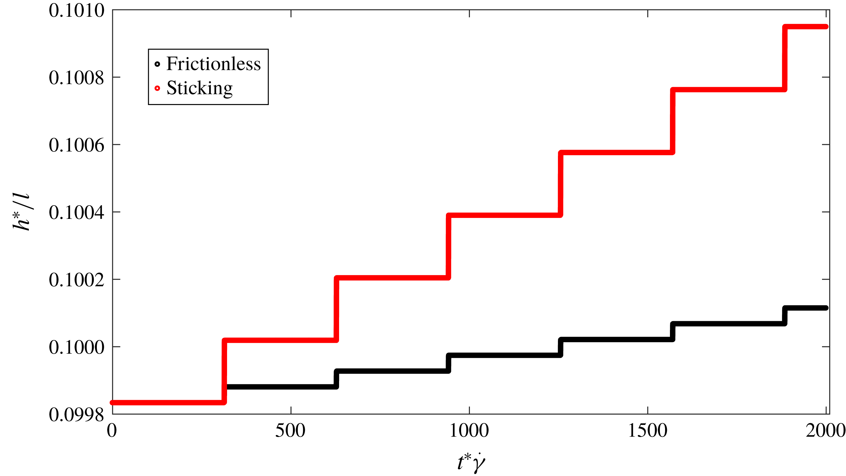
and significantly influence the fibre angles. To track the trajectory of the fibre due to all of these effects we integrate (3.9) with results supplied from (3.1), (3.2), (3.8) and the contact force. The choice of time steps is important in the trajectory evolution as both flipping and wall contact are very short-lived phenomena. The short-lived flipping can be expected from the Jeffery orbit component of (3.2) and evident from figure 5 showing evolution of
 $h$
. Based on the zero-inertia component of (3.2) flipping can be properly captured by choosing a time step of about
 $T/2\unicode[STIX]{x03C0}\unicode[STIX]{x1D705}$
. The wall contact is even shorter as it results from the small inertial perturbation of the fibre orbit between two successive wall contacts. An adaptive time stepping is used to capture the wall contact.
Wall contact occurs during a very small fraction of the orbital motion of the fibre, close to
 $\unicode[STIX]{x1D719}=-\unicode[STIX]{x03C0}/2$
and
 $\unicode[STIX]{x1D703}$
near its extrema of
 $\unicode[STIX]{x1D703}_{m}$
, but it is the sole pathway to increasing the height of the fibre. This is evident in figure 5, where
 $h$
behaves like a step function with the transitions corresponding to solid-body contact with the wall. These jumps at wall contact are additive. Eventually a fibre starting at any
 $0<h<1$
ends up at
 $h=1$
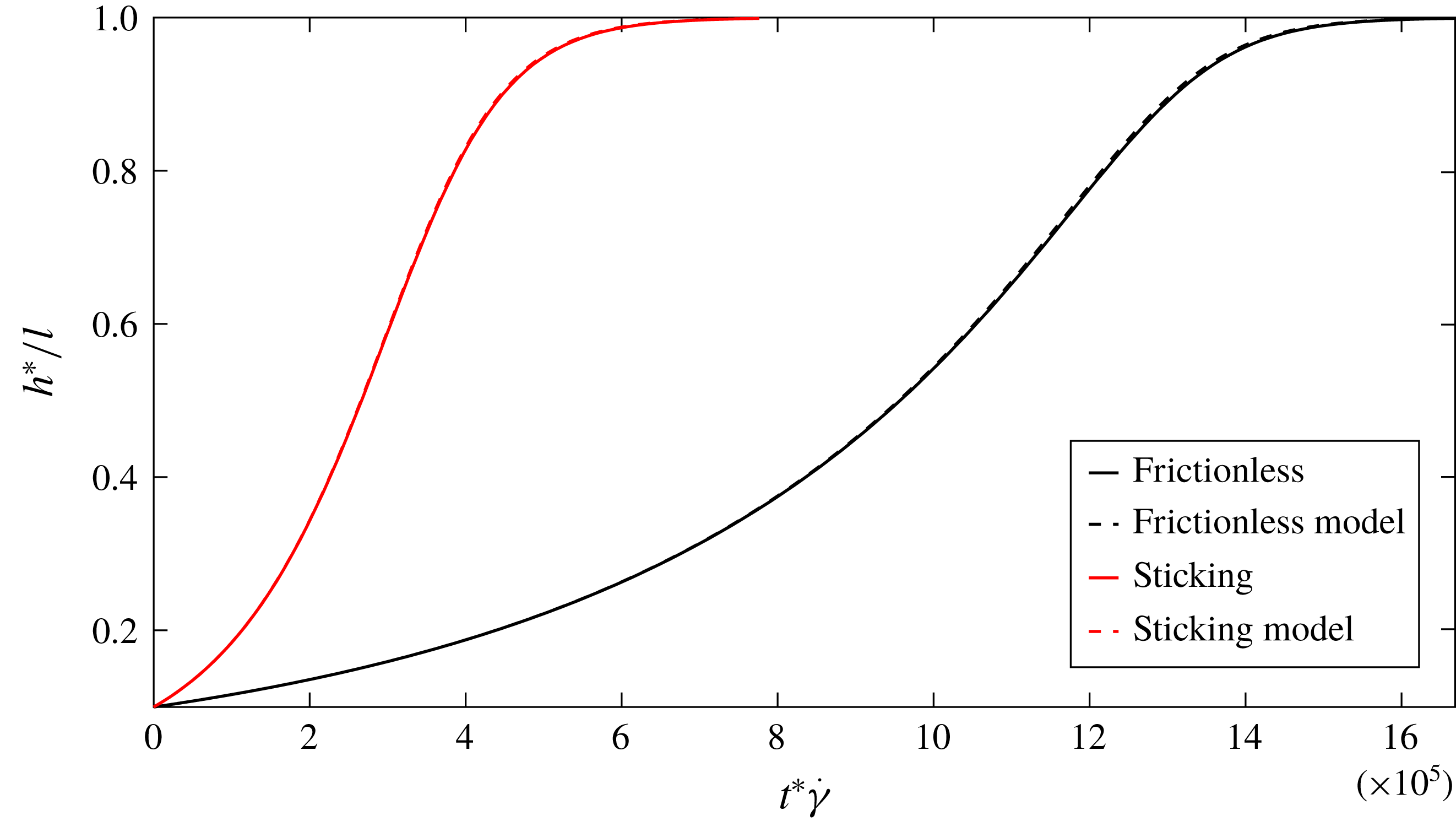
. This can be observed in figure 6, which shows the evolution of
 $h$
observed over a longer duration. The upward drift of the centre of mass of the fibre can be considered its lift velocity (
 $v_{l,N}$
). To obtain this lift velocity we consider a quasi-steady orbit that, for the given value of
 $h$
, just makes contact with the wall. In this configuration we will find the shift in the height of the centre of mass of a fibre and average it over the time period of the orbit to obtain the lift velocity. A model evolution based on this lift velocity
 $\text{d}h^{model}/\text{d}t=v_{l,N}(h^{model})$
agrees well with the full trajectory calculation, as evident from figure 6.
Trajectory of the fibre centre of mass for
 $\unicode[STIX]{x1D705}=100$
in a flow with
 $Re=10^{-3}$
shown over a long period of time. The rate at which the fibre moves away from the wall is faster for a sticking contact. The model evolution from (3.24) and (3.25) agrees well with the full simulation.

In the quasi-steady orbit model, we assume that the fibre makes contact with the wall at exactly
 $\unicode[STIX]{x1D719}=-\unicode[STIX]{x03C0}/2$
and
 $\unicode[STIX]{x1D703}=\unicode[STIX]{x1D703}_{m}$
. We evaluate the shift in height of the fibre using the kinematic constraint. This will capture the total drift of the fibre from the wall as it evolves in a sequence of quasi-steady orbits while the fibre end continues to brush the wall. The resulting evolution of the fibre centre of mass is
 $$\begin{eqnarray}\displaystyle \unicode[STIX]{x0394}h=-\cos \unicode[STIX]{x1D703}_{m}\unicode[STIX]{x0394}\unicode[STIX]{x1D703}. & & \displaystyle\end{eqnarray}$$
Here
 $\unicode[STIX]{x0394}\unicode[STIX]{x1D703}$
is the net change of
 $\unicode[STIX]{x1D703}$
during a Jeffery orbit. This includes effects of both the inertial drift
 $\unicode[STIX]{x0394}\unicode[STIX]{x1D703}_{I}$
and the wall contact
 $\unicode[STIX]{x0394}\unicode[STIX]{x1D703}_{N}$
. The perturbation to the fibre motion due to wall contact is captured through
 $\unicode[STIX]{x0394}\unicode[STIX]{x1D703}_{N}$
evaluated at
 $\unicode[STIX]{x1D719}=-\unicode[STIX]{x03C0}/2$
. For the case of frictionless contact this can be obtained from (3.11) as
 $$\begin{eqnarray}\displaystyle \frac{\unicode[STIX]{x0394}\unicode[STIX]{x1D703}_{N}}{\unicode[STIX]{x0394}h}=-\frac{3\cos \unicode[STIX]{x1D703}_{m}}{1+\sin ^{2}\unicode[STIX]{x1D703}_{m}}. & & \displaystyle\end{eqnarray}$$
For a sticking contact, from (3.13), at
 $\unicode[STIX]{x1D719}=-\unicode[STIX]{x03C0}/2$
it can be shown that
 $$\begin{eqnarray}\displaystyle \unicode[STIX]{x0394}\unicode[STIX]{x1D703}_{N}=0. & & \displaystyle\end{eqnarray}$$
The inertial perturbation to the quasi-steady Jeffery orbit between two consecutive wall contacts is found based on the change in
 $C$
between
 $\unicode[STIX]{x1D719}=-\unicode[STIX]{x03C0}/2$
and
 $\unicode[STIX]{x03C0}/2$
. To obtain this, first we consider the temporal evolution of
 $C$
that accounts for the effects of finite inertia. This is given as
 $$\begin{eqnarray}\displaystyle \hspace{-7.0pt}{\dot{C}}_{I}=\frac{Re\,C\unicode[STIX]{x1D716}^{\prime }}{2}2\sin ^{2}\unicode[STIX]{x1D703}\sin ^{2}\unicode[STIX]{x1D719}\cos ^{2}\unicode[STIX]{x1D719}\left[\frac{1}{30}+\frac{\unicode[STIX]{x1D705}^{2}}{\unicode[STIX]{x1D705}^{2}\sin ^{2}\unicode[STIX]{x1D719}+\cos ^{2}\unicode[STIX]{x1D719}}\left[\frac{\cos ^{2}\unicode[STIX]{x1D719}}{15}-\frac{\sin ^{2}\unicode[STIX]{x1D719}}{6}\right]\right].\quad & & \displaystyle\end{eqnarray}$$
Integrating over
 $\unicode[STIX]{x1D719}=-\unicode[STIX]{x03C0}/2$
to
 $\unicode[STIX]{x03C0}/2$
, which corresponds to motion over half of a Jeffery period, gives the change in orbit constant, due to inertial effects, to be
 $$\begin{eqnarray}\displaystyle \unicode[STIX]{x0394}C_{I}=\frac{\unicode[STIX]{x03C0}Re\,\unicode[STIX]{x1D705}\unicode[STIX]{x1D716}^{\prime }C}{30}\left[1+\frac{2}{\unicode[STIX]{x1D705}^{2}C^{2}}-2\sqrt{\frac{1}{\unicode[STIX]{x1D705}^{2}C^{2}}+\frac{1}{\unicode[STIX]{x1D705}^{4}C^{4}}}\right]. & & \displaystyle\end{eqnarray}$$
For slender fibres, the term
 $\unicode[STIX]{x1D705}C$
is large except in a very small portion of orientation space that corresponds to orbits close to the flow-vorticity plane. These orientations only predominate when
 $h$
is close to zero. Thus, we assume
 $\unicode[STIX]{x1D705}C\gg 1$
so that (3.18) reduces to
 $$\begin{eqnarray}\displaystyle \unicode[STIX]{x0394}C_{I}=\frac{\unicode[STIX]{x03C0}Re\,\unicode[STIX]{x1D705}\unicode[STIX]{x1D716}^{\prime }C}{30}. & & \displaystyle\end{eqnarray}$$
To relate this to a perturbation in
 $\unicode[STIX]{x1D703}$
we take the derivative of (3.3) at
 $\unicode[STIX]{x1D719}=-\unicode[STIX]{x03C0}/2$
. This gives
 $$\begin{eqnarray}\displaystyle \unicode[STIX]{x0394}\unicode[STIX]{x1D703}_{I}=\cos ^{2}\unicode[STIX]{x1D703}_{m}\unicode[STIX]{x0394}C_{I} & & \displaystyle\end{eqnarray}$$
so that
 $$\begin{eqnarray}\displaystyle \unicode[STIX]{x0394}\unicode[STIX]{x1D703}_{I}=\frac{\unicode[STIX]{x03C0}Re\,\unicode[STIX]{x1D705}\unicode[STIX]{x1D716}^{\prime }\sin \unicode[STIX]{x1D703}_{m}\cos \unicode[STIX]{x1D703}_{m}}{30}. & & \displaystyle\end{eqnarray}$$
We can now obtain the drift of the fibre by considering motion through half of a Jeffery orbit. For frictionless contact (3.14) along with inputs from (3.15) and (3.21) give
 $$\begin{eqnarray}\displaystyle \unicode[STIX]{x0394}h=-\cos \unicode[STIX]{x1D703}_{m}\left[\frac{\unicode[STIX]{x03C0}Re\,\unicode[STIX]{x1D705}\unicode[STIX]{x1D716}^{\prime }\sin \unicode[STIX]{x1D703}_{m}\cos \unicode[STIX]{x1D703}_{m}}{30}-\unicode[STIX]{x0394}h\frac{3\cos \unicode[STIX]{x1D703}_{m}}{1+\sin ^{2}\unicode[STIX]{x1D703}_{m}}\right]. & & \displaystyle\end{eqnarray}$$
Solving for
 $\unicode[STIX]{x0394}h$
and dividing by the Jeffery half-period (
 $\unicode[STIX]{x03C0}\unicode[STIX]{x1D705}$
, see (2.22) for the time period) gives the lift
 $$\begin{eqnarray}\displaystyle v_{l,N}(h)=\frac{Re\,\unicode[STIX]{x1D716}^{\prime }}{30}\left[\frac{\sin \unicode[STIX]{x1D703}_{m}\cos ^{2}\unicode[STIX]{x1D703}_{m}[1+\sin ^{2}\unicode[STIX]{x1D703}_{m}]}{4-2\sin ^{2}\unicode[STIX]{x1D703}_{m}}\right]. & & \displaystyle\end{eqnarray}$$
At wall contact and by extension throughout the Jeffery orbit, the height of the fibre is given as
 $\sin \unicode[STIX]{x1D703}_{m}=h$
. Thus,
 $$\begin{eqnarray}\displaystyle v_{l,N}(h)=\frac{Re\,\unicode[STIX]{x1D716}^{\prime }}{30}\left[\frac{h-h^{5}}{4-2h^{2}}\right]. & & \displaystyle\end{eqnarray}$$
For a sticking contact we can perform a similar analysis using (3.16) instead of (3.15). This gives
 $$\begin{eqnarray}\displaystyle v_{l,N}(h)=\frac{Re\,\unicode[STIX]{x1D716}^{\prime }}{30}\left[h-h^{3}\right]. & & \displaystyle\end{eqnarray}$$
Next, we rationalize the scaling of the lift velocity with wall contacts. All velocities are driven by the shear velocity
 $\dot{\unicode[STIX]{x1D6FE}}l$
. However, the orientational drift that drives wall collisions is a finite
 $Re$
effect caused by an
 $O(\unicode[STIX]{x1D716}^{\prime })$
disturbance velocity field that is important only during the
 $O(\unicode[STIX]{x1D705}^{-1})$
fraction of the time when the fibre is flipping, leading to an
 $O(\unicode[STIX]{x1D716}^{\prime }\unicode[STIX]{x1D705}^{-1}Re)$
factor. Thus, the scaling of the dimensional lift velocity
 $v_{l,N}^{\ast }$
due to contact and inertial orientation drift averaged over the Jeffery orbit is
 $\unicode[STIX]{x1D70C}\dot{\unicode[STIX]{x1D6FE}}^{2}l^{3}/(\unicode[STIX]{x1D707}\ln [l/a])$
.
Lift velocity experienced by the fibre for
 $h<1$
.

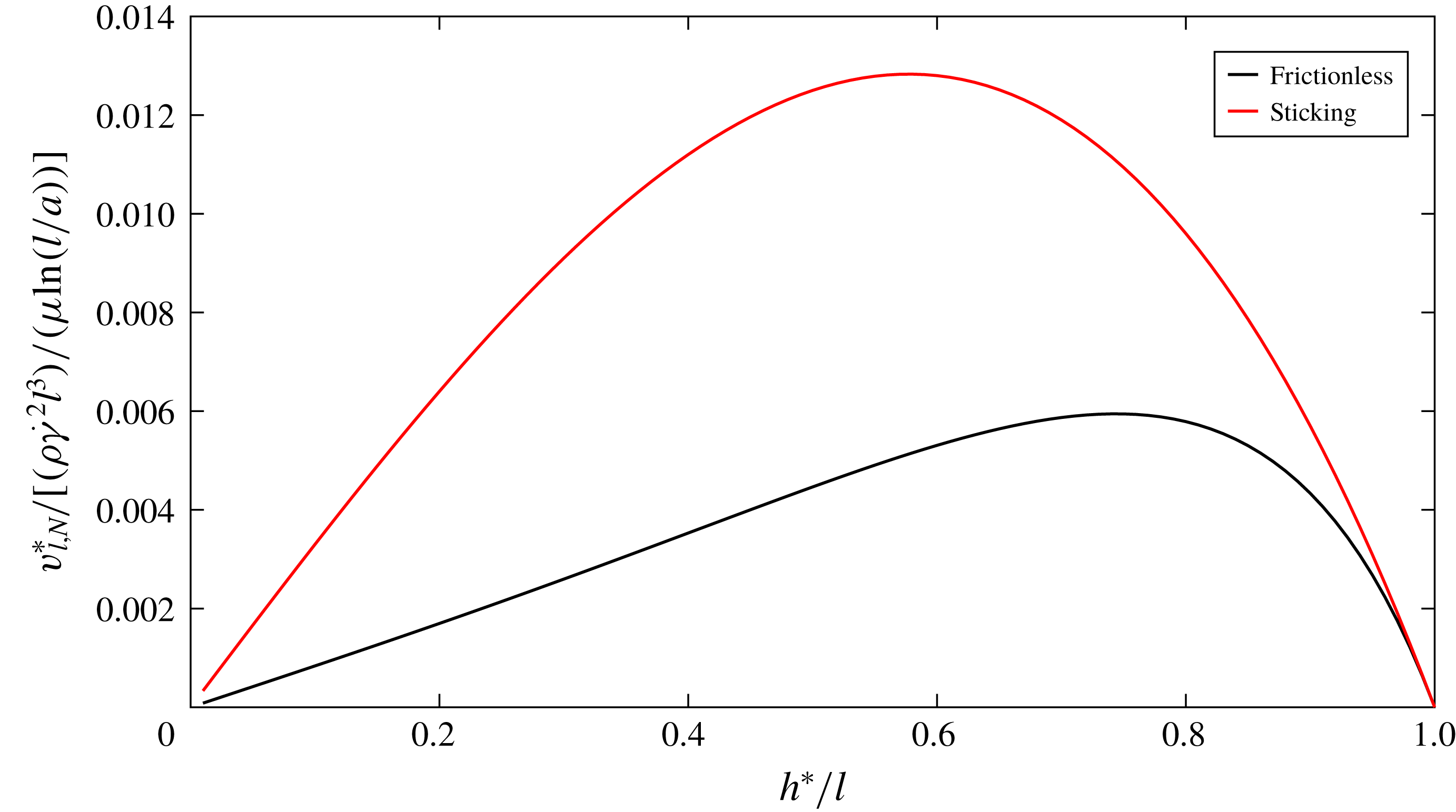
Figure 7 shows the variation of wall contact lift velocity as a function of the height of the centre of the fibre for both the sticking case and the frictionless contact. The lift velocity is small near
 $h=0$
, because the fibre is confined to orbits close to the flow-vorticity plane where its fluid velocity disturbance and inertial rotation are small. The lift velocity for a frictionless solid-body contact grows approximately linearly with
 $h$
until
 $h\approx 0.7$
. Beyond this height, the change of orientation and lift velocity diminish as the fibre approaches the flow-gradient plane. All the important features are observed for the sticking case as well but with a higher magnitude of lift velocity at all
 $h$
and shifted peak location.
In figure 6 we compare the evolution of the centre of mass of the fibre obtained by tracking the trajectory with
 $\text{d}h^{model}/\text{d}t=v_{l,N}(h^{model})$
. It can be seen that the model captures the change in position accurately for both the frictionless and sticking contacts. This confirms that at small Reynolds number, the constraint set by the accessible orbits that do not penetrate the wall captures the change of position obtained using a full description of the contact event.
There is a significant difference in fibre evolution between sticking and frictionless contact. To understand this we consider how the fibre orientation drift due to inertia, over the whole Jeffery orbit, is converted to positional displacement during the short-lived solid-body contact. A sticking contact allows the pole vaulting fibre to push its centre of mass a way from the wall efficiently using the large normal contact force needed to prevent the rotational motion from pushing the fibre end into the wall. A fibre with a frictionless contact has an additional tangent translational motion associated with the sliding of the contact which accommodates part of the fibre rotation with a smaller normal contact force and normal displacement. Thus we expect reduced net displacement from the wall for frictionless contact relative to the sticking case. This is reflected in the fibre evolution profiles and the analytically derived lift velocities.
The lift velocity presented in this section is driven by inertial drift of orientation and wall-contact-driven pole vaulting that breaks Stokes flow reversibility. This lift velocity is stronger by a factor of
 $\unicode[STIX]{x1D705}$
when compared to translation induced by inertia that was discussed in § 2. Thus, to leading order, the direct effect of inertial drift of the centre of mass of the fibre does not contribute to the wall contact lift velocity or the fibre dynamics in the
 $h<1$
regime.
4 Discussion
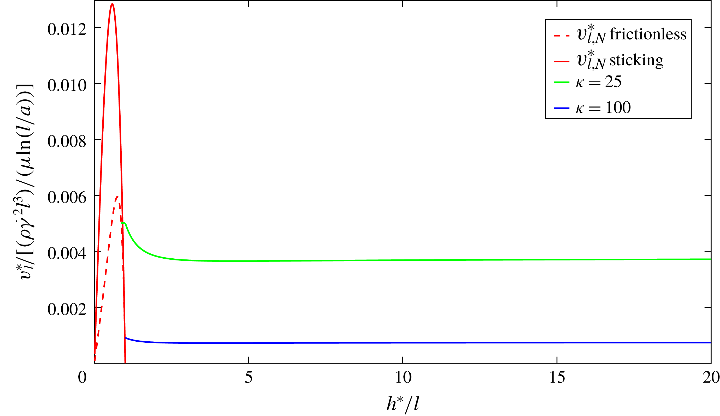
In the previous sections we have discussed the behaviour of a fibre migrating away from a wall in shear flow in two regions: one where the fibre makes contact with the wall and one where it rotates freely in the shear flow. We now combine the results of the two previous sections and present the variation of lift velocity over the whole inner region
 $h^{\ast }\ll L_{0}$
as a function of the non-dimensionalized distance of the centre of the fibre from the wall in figure 8. In this plot the lift velocity is scaled as
 $\unicode[STIX]{x1D70C}\dot{\unicode[STIX]{x1D6FE}}^{2}l^{3}/(\unicode[STIX]{x1D707}\ln [l/a])$
and is shown at two values of
 $\unicode[STIX]{x1D705}$
. The global peak of the scaled lift velocity occurs at
 $h<1$
even at a moderate aspect ratio of 25 and the frictionless case. This is expected as the inertial lift force on a freely suspended fibre is weaker than the contact force driven by the inertial drift of orientation. This contact driven motion diminishes to zero due to the driving force becoming less and less effective as
 $h\rightarrow 1^{-}$
. Thus, there is a thin
 $O(1/\unicode[STIX]{x1D705})$
region around
 $h\rightarrow 1^{-}$
where the fibre makes contact with the wall but the inertially induced translational velocity is the dominant contributor to the lift velocity. In figure 8, the lift velocity in this very small region is approximated by the value computed for
 $h\rightarrow 1^{+}$
.
Variation of lift velocity
 $v_{l}$
over the inner region, at aspect ratios of 25 and 100. For
 $h>1$
the curves are in ascending order of aspect ratio going from top to bottom. For
 $h<1$
the scaled velocity is independent of aspect ratio and both the sticking and frictionless contact cases are shown.

To complete the description of the manner in which the lift velocity varies with
 $h$
, we briefly consider the lift velocity in the outer region
 $h^{\ast }\geqslant O(L_{0})$
. Although a detailed analysis of lift on a fibre has not been performed in this region, it can be noted that the qualitative dependence of the lift velocity on
 $h$
is likely to be similar to that for spheres, because both can be viewed as point-force dipoles on the length scale
 $L_{0}$
, although the force dipole of a fibre varies periodically with time. McLaughlin (Reference McLaughlin1993) showed that the lift force on a sphere has a maximum nearly equal to the large separation asymptote of the inner region, when
 $l\ll h^{\ast }\ll L_{0}$
, and decays with wall separation in the outer region. It is reasonable to expect that the lift velocity of fibres exhibits a similar behaviour. Since the lift velocity maximum of the outer region corresponds to the inner region asymptote, it can be inferred that the maximum at
 $h\approx 0.7$
is likely to be the global maximum for high-aspect-ratio fibres for all forms of contact while the value
 $0.03\unicode[STIX]{x1D70C}\dot{\unicode[STIX]{x1D6FE}}^{2}l^{2}a/(\unicode[STIX]{x1D707}\ln [2l/a])$
will be the global maximum lift velocity without wall contact.
Hydrodynamic lift on a fibre in wall-bounded shear flow is applicable to the design of cross-flow filtration. Cross-flow filtration is performed by flowing a suspension of particles through a channel or tube with a fluid filtrate drawn out through the porous walls. In conventional operation, the pores of the membrane block the passage of the particles, while transport processes in the channel including hydrodynamic lift, shear-induced hydrodynamic diffusion and molecular diffusion limit the accumulation of particles at the membrane surface (see Altena & Belfort Reference Altena and Belfort1984). Transport is the dominant filtration mechanism in sieve-free operation of cross-flow filtration where pores are large enough to pass the particles, and only transport mechanisms, such as inertial lift, prevent particles from flowing through the membrane with the filtrate (see Belfort et al. Reference Belfort, Davis and Zydney1994; Hurwitz & Brantley Reference Hurwitz and Brantley2000). This mode of operation has the advantage of reducing fouling and being less sensitive to colloidal interactions between the particles and the wall. In microfluidic separation the transport mechanism is exploited to focus the particles in certain regions of the channel, with bifurcation of the channel achieving the desired separation. This focusing can be achieved by inertial lift (see Di Carlo et al. Reference Di Carlo, Edd, Irimia, Tompkins and Toner2008; Masaeli et al. Reference Masaeli, Sollier, Amini, Mao, Camacho, Doshi, Mitragotri, Alexeev and Di Carlo2012). Thus, our analysis of hydrodynamic inertial lift will inform microfluidic separators.
In experiments on microfluidic separation by Masaeli et al. (Reference Masaeli, Sollier, Amini, Mao, Camacho, Doshi, Mitragotri, Alexeev and Di Carlo2012), particles with small Reynolds number, from 0.3 to 0.75, have been shown to inertially focus in certain regions of the channel. The asymptotic
 $Re$
results of our study will inform particle transport in these conditions. This is expected as an equivalent calculation on spheres by Hood, Lee & Roper (Reference Hood, Lee and Roper2015) showed that inertial lift force is governed by the asymptotic
 $Re$
result for particle Reynolds number as high as 10. At higher
 $Re$
, fibre motion can potentially halt due to competition between Jeffery orbit rotation and inertia. Subramanian & Koch (Reference Subramanian and Koch2005) showed that this will happen above a critical Reynolds number
 $Re_{m}=30\ln (\unicode[STIX]{x1D705})/\unicode[STIX]{x1D705}$
. The moderate-aspect-ratio particles studied by Masaeli et al. (Reference Masaeli, Sollier, Amini, Mao, Camacho, Doshi, Mitragotri, Alexeev and Di Carlo2012) fall outside the range for which slender-body theory is quantitatively accurate. However, by keeping terms of
 $O(1/(\ln \unicode[STIX]{x1D705})^{2})$
, the present study provides qualitative insight into phenomena that become more important at moderate aspect ratio, including wall reflections, oscillatory translation of non-spherical particles perpendicular to the wall, inertially induced breaking of the symmetry of finite-aspect-ratio particle rotation and the effects of the precise variation of particle thickness as captured by the
 $\ln [(1-s^{2})^{1/2}/a(s)]$
term in (2.14).
For sieve-free operation of cross-flow filtration, Levesley & Bellhouse (Reference Levesley and Bellhouse1993) performed experiments on sub-millimetre-diameter particles and demonstrated inertial-lift-driven separation. Common targets for filtration, however, are micrometric and experiments by Subramony (Reference Subramony2017) demonstrated the importance of inertial lift for these particle sizes. While these studies focus on separation by size, the extent of non-sphericity can act also as a distinguishing feature in filtration. Our study provides the analytical framework for such an approach. This approach will be of particular interest to micrometre-sized biological and industrial particles with non-spherical shapes (see Masaeli et al. Reference Masaeli, Sollier, Amini, Mao, Camacho, Doshi, Mitragotri, Alexeev and Di Carlo2012).
To understand how design of cross-flow filtration is informed by the results of our study we consider the profile of the lift velocity as a function of
 $h$
as described in figure 8. This can determine the position at which particles would concentrate as a result of the balance of lift and permeate velocities. If the permeate velocity is sufficiently small, the particles will remain in the outer region
 $h^{\ast }>L_{0}$
far from the membrane. As the permeate velocity is increased, the wall separation of the fibres will decrease gradually until the permeate velocity reaches the value
 $0.0303\unicode[STIX]{x1D70C}\dot{\unicode[STIX]{x1D6FE}}^{2}l^{2}a/(\unicode[STIX]{x1D707}\ln [2l/a])$
corresponding to the maximum lift velocity occurring in the matching region
 $l\ll h^{\ast }\ll L_{0}$
. When the permeate velocity exceeds this value, the concentrated band will jump to a position near
 $h=1$
in which the fibres make contact with the wall. If we take an example of a filtration system where the permeate velocity is
 $20~\unicode[STIX]{x03BC}\text{m}~\text{s}^{-1}$
and the shear rate is
 $\dot{\unicode[STIX]{x1D6FE}}=6\times 10^{4}~\text{s}^{-1}$
with filtrate and particle characteristics
 $\unicode[STIX]{x1D70C}=10^{3}~\text{kg}~\text{m}^{-3},\unicode[STIX]{x1D707}=10^{-3}~\text{Pa}~\text{s},l=2~\unicode[STIX]{x03BC}\text{m}$
and
 $\unicode[STIX]{x1D705}=10$
, the resultant maximum lift velocity without contact is about
 $29~\unicode[STIX]{x03BC}\text{m}~\text{s}^{-1}$
and the particle is retained in the channel. If the permeate velocity is increased, say to
 $50~\unicode[STIX]{x03BC}\text{m}~\text{s}^{-1}$
, the non-spherical particle is pushed towards the membrane that acts as the wall. At this boundary, however, the lift velocity is
 $75~\unicode[STIX]{x03BC}\text{m}~\text{s}^{-1}$
for frictionless contacts and
 $163~\unicode[STIX]{x03BC}\text{m}~\text{s}^{-1}$
for sticking contacts. The permeate velocity could be increased to substantially higher values but the retention of the fibres in the channel would depend on the details of the collisions of fibres with a porous boundary. The degree to which spherical particles can be retained in a porous channel due to their excluded volume interactions with the wall has been studied theoretically by Yan, Acrivos & Weinbaum (Reference Yan, Acrivos and Weinbaum1991) and experimentally by Van Dinther et al. (Reference Van Dinther, Schroën, Imhof, Vollebregt and Boom2013). No comparable analysis has yet been performed for non-spherical particles whose interactions with the pores can play an important role, especially if they are of comparable size, as is typical in sieve-free operation.
Our study has provided insight into the role of non-sphericity in inertial drift. Many real-world targets of sieve-free cross-flow filtration, microfluidic separators and other systems that rely on inertia-induced transport exhibit some degree of deviation from ideal spheres. Instead of treating non-sphericity as a hindrance, our study paves the way to exploit it to achieve better outcomes. Our study also combines the non-hydrodynamic wall contact forces with inertial effects. This will provide a framework for future studies that look at particle geometry with wall effects.
5 Conclusions
We have studied the hydrodynamic lift velocity of a neutrally buoyant fibre in the presence of a wall at small, but finite, Reynolds number. While the lift of spheres has been studied extensively, this is the first analytical study of the lift on non-spherical, neutrally buoyant particles in wall-bounded shear flow. The disturbance fluid velocity is dominated by viscous effects provided that
 $h^{\ast }<L_{0}$
. Thus the lift due to inertial effects can be obtained as a regular perturbation of the Navier–Stokes equation in terms of Reynolds number. The lift velocity has a strong dependence on geometry. The non-sphericity allows for wall contact and the fibre lift velocity, when
 $a<h^{\ast }<l$
, is dominated by its interactions with the wall. An equivalent case does not exist for a sphere.
For a freely rotating fibre with
 $h^{\ast }>l$
, the lift velocity arises from the asymmetry of the flow around the fibre induced by inertial effects. In §2, we used a generalized reciprocal theorem to capture the first effects of inertia on the fibre velocity in terms of integrals involving the Stokes velocity field of a fibre in wall-bounded shear flow and a Stokes comparison problem with a fibre experiencing a force normal to the wall. The force distribution on the fibre was evaluated using slender-body theory and retaining non-dimensional forces per unit length of the fibre of
 $O(1/(\ln 2\unicode[STIX]{x1D705}))$
and
 $O(1/[\ln 2\unicode[STIX]{x1D705}]^{2})$
. The boundary conditions on the wall were satisfied using the wall reflection image singularities associated with a Stokeslet as determined by Blake & Chwang (Reference Blake and Chwang1974). The retention of
 $O(1/[\ln 2\unicode[STIX]{x1D705}]^{2})$
forces is required to obtain quantitatively accurate predictions even for aspect ratios as high as
 $10^{4}$
. Terms of this order also capture a number of qualitative features that are not present at
 $O(1/(\ln 2\unicode[STIX]{x1D705}))$
including a complex interaction of the fibre geometry with the imposed shear flow, the modification of the fibre force distribution due to wall interactions, the oscillatory motion of the fibre perpendicular to the wall and the inertia-induced asymmetry of fibre rotation.
While the lift velocity of a sphere depends only on its distance from the wall, the lift velocity of a fibre depends on the wall separation as well as the fibre orientation. The force distribution on a fibre, driving the lift velocity, changes as it rotates in the shear flow. The temporal dynamics thus becomes important and is captured by Jeffery orbits. In particular, the Jeffery orbit
 $C=\infty$
, corresponding to rotation in the flow-gradient plane, was shown by Subramanian & Koch (Reference Subramanian and Koch2005) to be the preferred configuration when fluid inertia is present. A high-aspect-ratio fibre spends most of its time nearly aligned with the flow direction making a very small fluid velocity disturbance and an
 $O(\unicode[STIX]{x1D705}^{-1})$
fraction of its orbit rotating through other orientations where it makes a larger disturbance. This behaviour causes the time-averaged lift velocity to be a factor of
 $\unicode[STIX]{x1D705}^{-1}$
smaller than the value for a sphere with the same maximum dimension. The fibre lift velocity is reduced further by a factor of
 $1/(\ln 2\unicode[STIX]{x1D705})$
due to the small magnitude of the velocity disturbance of a slender body even when its axis has a substantial projection along the extensional axis of the imposed flow. These two factors cause the fibre lift velocity to have a non-trivial scaling with its half-length
 $l$
and radius
 $a$
and to reach a maximum value, for
 $l\ll h^{\ast }\ll L_{0}$
, of
 $0.0303\unicode[STIX]{x1D70C}\dot{\unicode[STIX]{x1D6FE}}^{2}l^{2}a/(\unicode[STIX]{x1D707}\ln [2l/a])$
in contrast to the simpler result of
 $0.1\unicode[STIX]{x1D70C}\dot{\unicode[STIX]{x1D6FE}}^{2}a^{3}/\unicode[STIX]{x1D707}$
for a sphere. A further qualitative difference between the lift velocity of a fibre and a sphere is that the lift velocity of a fibre changes by only a small amount as
 $h^{\ast }\rightarrow l$
, while the lift velocity of a sphere vanishes as
 $h^{\ast }\rightarrow a$
. This difference arises because the hydrodynamic resistance to translation of the fibre normal to the wall remains finite because of its thin cross-section and sharp edges, while the lubrication resistance to normal motion of the sphere diverges.
Our study in § 3 is the first to analyse the coupled effects of fluid-inertia-induced orientational changes and pole vaulting of fibres due to wall contact. To account for the various types of solid-body interactions with the wall we consider frictionless and sticking contacts. All solid-body contacts between fibre and wall push the fibre away from the wall and, if it is out of the flow-gradient plane, to an orbit further out of the plane. Inertial drift tends to bring the fibre to an orbit closer to the flow-gradient plane. The interplay of these two effects can be modelled as causing the fibre to drift across a sequence of quasi-steady orbits producing a net lift velocity. A detailed simulation of the orientational and translational trajectory of a fibre during wall contact was shown to be in good agreement with a model trajectory based on the quasi-steady orbit approximation. The scaling of the lift velocity due to wall contacts for
 $a<h^{\ast }<l$
was found to be
 $\unicode[STIX]{x1D70C}\dot{\unicode[STIX]{x1D6FE}}^{2}l^{3}/(\unicode[STIX]{x1D707}\ln [l/a])$
which is larger than the case for no wall contact by a factor of the aspect ratio. This analytically derived lift velocity showed an initial increase which is almost linear with distance from the wall, then reached a maximum of about
 $0.013\unicode[STIX]{x1D70C}\dot{\unicode[STIX]{x1D6FE}}^{2}l^{3}/(\unicode[STIX]{x1D707}\ln [l/a])$
for the sticking contact and
 $0.006\unicode[STIX]{x1D70C}\dot{\unicode[STIX]{x1D6FE}}^{2}l^{3}/(\unicode[STIX]{x1D707}\ln [l/a])$
for the frictionless contact, and decreased to zero as
 $h\rightarrow 1$
. This maximum was shown to be the global maximum even for fibres of moderate
 $\unicode[STIX]{x1D705}$
in § 4.
The lift velocity finds application in industrial processes such as cross-flow filtration and in laboratory processes including microfluidic separation. In § 4 we briefly described how knowledge of the lift velocity can be used to better control particle separations in flow channels. In cross-flow filtration the results can be used to design a separation based on shape as well as size and one that does not rely upon the detailed interaction of the particles with the porous membrane. Criteria were derived for the shear rate and permeate velocity range which retains particles within the bulk of the channel as well as a range that leads to pole vaulting on the membrane surface. These criteria make a distinction based on geometry and will be useful in many industrial and laboratory systems where the target particles are not spherical.
Acknowledgements
This work was supported by NSF-CBET grant 1505795.