





1. Introduction
Travelling periodic waves on the surface of an irrotational fluid under the gravity force are called Stokes waves [Reference Stokes46, Reference Stokes47]. The mathematical theory of their existence was elaborated in [Reference Levi-Civita31, Reference Nekrasov40, Reference Struik48]. The family of Stokes waves with smooth profiles is continued towards a limit, in which the wave profile becomes peaked with a specific 120 $^{o}$ angle at the crest. The existence of the limiting wave with the peaked profile was proven in [Reference Amick, Fraenkel and Toland1, Reference Plotnikov43, Reference Toland51].
The potential motion of a two-dimensional fluid is described by the classical Euler’s equations. Although many equivalent formulations are known for Euler’s equations, we will particularly address the formulation involving pseudo-differential operators in conformal variables. When the fluid is considered to be infinitely deep, the conformal transformation maps the vertical semi-strip to the fluid domain and does not depend on the mean value of the fluid surface in conformal variables. This formulation leads to Babenko’s pseudo-differential equation [Reference Babenko2], which was used in the studies of travelling waves with both smooth and peaked profiles [Reference Balk3, Reference Dyachenko, Kuznetsov, Spector and Zakharov19, Reference Dyachenko, Lushnikov and Korotkevich22, Reference Locke and Pelinovsky33].
Based on global bifurcation theory and analysis of the pseudo-differential operators, several important results on the existence of Stokes waves were rigorously justified in [Reference Buffoni, Dancer and Toland10, Reference Buffoni, Dancer and Toland11, Reference Plotnikov42]. It was shown in [Reference Buffoni, Dancer and Toland11] that there exist infinitely many bifurcation points for the family of travelling periodic waves when it is extended towards the highest-peaked wave. These points are identified as zero eigenvalues of the associated self-adjoint (Hessian) operator related to the variational formulation. They correspond to the extremal points of the wave speed versus wave steepness. The Morse index, which is the number of negative eigenvalues of the Hessian operator in the space of co-periodic perturbations, becomes arbitrarily large in the limit of the highest-peaked wave [Reference Plotnikov42]. Based on the band-gap structure of the spectrum of the linearized operator with periodic coefficients, it was also shown in [Reference Buffoni, Dancer and Toland11] that there are infinitely many subharmonic bifurcation points. These bifurcation points are identified as zero eigenvalues of the Hessian operator with respect to perturbations of multiple periods. Construction of travelling waves past the subharmonic bifurcation points via continuation was recently shown in [Reference Semenova45].
The global bifurcation theory is also related to the stability theory for Stokes waves. Stability of periodic waves with respect to co-periodic perturbations was studied numerically in [Reference Longuet-Higgins and Tanaka34–Reference Longuet-Higgins36, Reference Saffman44, Reference Tanaka49, Reference Tanaka50]. It was realized in [Reference Saffman44, Reference Tanaka50] that the new unstable eigenvalues in the linearized stability problem appear at the extremal points of the wave energy, rather than at the extremal points of the wave speed. In [Reference Dyachenko and Pelinovsky20], we proved this conjecture based on analysis of the pseudo-differential operators in conformal variables and also showed that the extremal points of the wave energy coincide with the extremal points of the horizontal momentum.
Finally, the modulational stability problem is defined by the spectrum of the linearized operators with respect to perturbations of longer periods. The modulational instability of small-amplitude Stokes waves, also known as the Benjamin–Feir instability [Reference Benjamin and Feir4, Reference Zakharov52], was studied in [Reference Berti, Maspero and Ventura6–Reference Bridges and Mielke8, Reference Creedon and Deconinck14, Reference Hur and Yang27, Reference Nguyen and Strauss41]. Additionally, the high-frequency instabilities of small-amplitude Stokes waves were studied for the same spectral problem in [Reference Berti, Maspero and Ventura6, Reference Creedon, Deconinck and Trichtchenko13, Reference Deconinck and Oliveras18].
Numerical solutions of the modulational stability problem for Stokes waves of increasing steepness have been recently developed with high accuracy in [Reference Dyachenko, Hur and Silantyev21, Reference Dyachenko and Semenova23, Reference Dyachenko and Semenova24, Reference Korotkevich, Lushnikov, Semenova and Dyachenko29, Reference Korotkevich and Prokofiev30, Reference Murashige and Choi39]. The recent comprehensive studies in [Reference Deconinck, Dyachenko, Lushnikov and Semenova16, Reference Deconinck, Dyachenko and Semenova17] showed that there exist four fundamental bifurcations of the spectral bands near the origin, which are repeated recurrently when the family of Stokes waves is increased towards the highest-peaked wave. The four bifurcations are observed in the following order: (a) new figure-8 bands appearing at each extremal point of speed, (b) degeneration of figure-8 bands resulting in their vertical slope, (c) new circular bands around the origin appearing at each period-doubling bifurcation and (d) reconnection of figure- $\infty$ bands at each extremal point of energy. The necessity of infinitely many bifurcation points for (a) and (c) is proven in [Reference Buffoni, Dancer and Toland11]. The bifurcation points for (d) were studied in [Reference Dyachenko and Pelinovsky20]. The bifurcation points for (b) have not been seen in the previous work on the modulational stability problem in toy models for fluids [Reference Bronski, Hur and Marangell9, Reference Cui and Pelinovsky15]. A similar pattern of recurrent bifurcations was also reported for Stokes waves in a finite-depth fluid [Reference Byrnes, Deconinck and Semenova12].
It is the purpose of this work to study rigorously the modulational stability problem associated with the pseudo-differential operators in conformal variables and to derive the criteria and the normal forms for the four bifurcations near the origin. We also compute coefficients of the normal forms numerically for the first and second bifurcation cycles to show an excellent agreement between the normal forms and the numerical approximations of spectral bands near the origin.
1.1. Equations of motion in conformal variables
Let 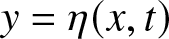 $y = \eta(x,t)$ be the profile for the free surface of an incompressible and irrotational deep fluid in the
 $2\pi$-periodic domain
 $\mathbb{T}$ that depends on time
 $t \in \mathbb{R}$. For a proper definition of the free surface, we add the zero-mean constraint
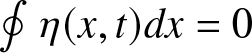 $\oint \eta(x,t) dx = 0$, which is invariant in the time evolution of Euler’s equations. Here and in what follows, the symbol
 $\oint$ denotes an integral of a periodic function over the period, which is independent of the limits of integration. We use the notation
 $L^2_{\rm per}$ for
 $2\pi$-periodic squared-integrable functions and similarly,
 $H^1_{\rm per}$ for
 $2\pi$-periodic squared-integrable functions with squared-integrable first derivatives.
Let  $z(u,t) = \xi(u,t) + i\eta(u,t)$ be a holomorphic function, which maps the vertical strip in the lower complex half-plane
 $\mathbb{T} \times i(-\infty,0]$ to the fluid domain beneath the free surface at
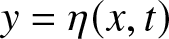 $y = \eta(x,t)$. The top boundary
 $\mbox{Im}\,u = 0$ gives the surface profile in the parametric form:
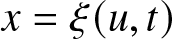 $x = \xi(u,t)$ and
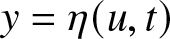 $y = \eta(u,t)$, where
 $u \in \mathbb{T}$ and
 $t \in \mathbb{R}$. The conformal mapping yields the relation
 \begin{equation}
\xi = u - \mathcal{H} \eta,
\end{equation}
where  $\mathcal{H}$ is the periodic Hilbert transform, a skew-adjoint bounded operator in
 $L^2_{\rm per}$, normalized by the Fourier symbol
 \begin{equation}
\hat{\mathcal{H}}_n = \left\{\begin{array}{ll}
i \; {\rm sgn}(n), \quad & n \in \mathbb{Z} \backslash \{0\}, \\
0, \quad & n = 0. \end{array} \right.
\end{equation}
It follows from (1.1) that
 \begin{equation*}
\xi_u = 1 + \mathcal{K} \eta \quad \mbox{and} \quad \xi_t = -\mathcal{H}\eta_t,
\end{equation*}
where  $\mathcal{K} = - \mathcal{H} \partial_u = |\partial_u|$ is a positive self-adjoint operator in
 $L^2_{\rm per}$ with the domain
 $H^1_{\rm per}$ and the Fourier symbol
 \begin{equation}
\hat{\mathcal{K}}_n = |n|, \quad n \in \mathbb{Z}.
\end{equation}
Derivation of equations of motion in conformal variables can be found in Appendices of [Reference Dyachenko, Lushnikov and Korotkevich22, Reference Locke and Pelinovsky32]. These equations can be written as the system of pseudo-differential equations for the velocity potential  $\psi$ and the free surface
 $\eta$ defined at the top boundary
 $\mbox{Im}\,u = 0$:
 \begin{equation}
\left\{\begin{array}{l}
\eta_t (1 + \mathcal{K} \eta) + \eta_u \mathcal{H} \eta_t + \mathcal{H} \psi_u = 0, \\
\psi_t \eta_u - \psi_u \eta_t + \eta \eta_u + \mathcal{H} \left( (1 + \mathcal{K} \eta) \psi_t +
\psi_u \mathcal{H} \eta_t + \eta (1 + \mathcal{K} \eta) \right) = 0,
\end{array}
\right. \quad u \in \mathbb{T}.
\end{equation}
The system (1.4) admits the following conserved quantities, e.g., see [Reference Benjamin and Olver5] and [Reference Dyachenko and Pelinovsky20]:
 \begin{equation}
M(\eta) = \frac{1}{2\pi} \oint \eta (1+ \mathcal{K} \eta) du,
\end{equation}
 \begin{equation}
P(\psi,\eta) = - \frac{1}{2\pi} \oint \psi \eta_u du,
\end{equation}
 \begin{equation}
Q(\psi,\eta) = \frac{1}{2\pi} \oint \psi (1 + \mathcal{K} \eta) du,
\end{equation}
 \begin{equation}
H(\psi,\eta) = \frac{1}{4\pi} \oint \left( \psi \mathcal{K} \psi + \eta^2 (1 + \mathcal{K} \eta) \right) du,
\end{equation}
which are referred to as mass, horizontal momentum, vertical momentum and energy, respectively. Due to the zero-mean constraint 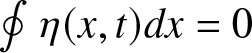 $\oint \eta(x,t) dx = 0$ on the surface elevation
 $\eta$ and the chain rule
 $dx = (1 + \mathcal{K} \eta) du$, we get the constraint
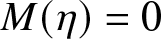 $M(\eta) = 0$, or explicitly, from (1.5),
 \begin{equation}
\oint \eta (1+ \mathcal{K} \eta) du = 0.
\end{equation}
In the reference frame moving with the wave speed  $c$, the system (1.4) with the constraint (1.9) can be rewritten as
 \begin{equation}
\left\{\begin{array}{l}
\eta_t (1 + \mathcal{K} \eta) + \eta_u \mathcal{H} \eta_t = \mathcal{K} \zeta, \\
\zeta_t (1 + \mathcal{K} \eta) + \zeta_u \mathcal{H} \eta_t - \mathcal{H} (\zeta_t \eta_u - \zeta_u \eta_t ) - 2 c \mathcal{H} \eta_t = \left(c^2 \mathcal{K} - 1\right)\eta - \eta \mathcal{K} \eta - \frac{1}{2} \mathcal{K} \eta^2,
\end{array}
\right.
\end{equation}
where the potential  $\psi$ has been transformed to
 $\zeta$ by using
 $\psi = -c \mathcal{H} \eta + \zeta$ and the variable
 $u$ stands now for
 $u - ct$.
Travelling waves correspond to the reduction  $\zeta = 0$ and
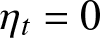 $\eta_t = 0$ in the system (1.10). This gives the scalar pseudo-differential Babenko’s equation for the
 $2\pi$-periodic profile
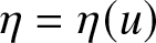 $\eta = \eta(u)$:
 \begin{equation}
(c^2 \mathcal{K} - 1) \eta = \frac{1}{2} \mathcal{K} \eta^2 + \eta \mathcal{K} \eta.
\end{equation}
This equation can be obtained as the Euler–Lagrange equation for the action functional
 \begin{equation}
\Lambda_c(\eta) := \frac{1}{2} \langle (c^2 \mathcal{K} - 1) \eta, \eta \rangle -
\frac{1}{2} \langle \mathcal{K} \eta^2, \eta \rangle,
\end{equation}
where  $\langle f, g \rangle := \frac{1}{2\pi} \oint \bar{f}(u) g(u) du$ is the normalized inner product in
 $L^2_{\rm per}$.
It was shown in [Reference Buffoni, Dancer and Toland10, Reference Buffoni, Dancer and Toland11] that there exists a family of smooth travelling waves with the even profile 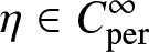 $\eta \in C^{\infty}_{\rm per}$ satisfying the Babenko equation (1.11) for
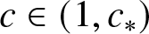 $c \in (1,c_*)$ with some
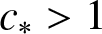 $c_* \gt 1$. The left end
 $c = 1$ of the interval
 $(1,c_*)$ is a local bifurcation point of the
 $2\pi$-periodic solutions from the zero solution. The even single-lobe profile
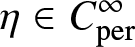 $\eta \in C^{\infty}_{\rm per}$ is approximated near
 $c = 1$ by the following small-amplitude expansion [Reference Creedon and Deconinck14, Reference Dyachenko, Kuznetsov, Spector and Zakharov19]:
 \begin{equation}
\eta = a \cos(u) + a^2 \left[ \cos(2u) - \frac{1}{2} \right] + \frac{3}{2} a^3 \cos(3u) + \mathcal{O}(a^4)
\end{equation}
and
 \begin{equation}
c^2 = 1 + a^2 + \mathcal{O}(a^4),
\end{equation}
where  $a \in \mathbb{R}$ is the amplitude parameter. The parameter
 $a \gt 0$ measures the steepness of the travelling wave profile
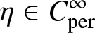 $\eta \in C^{\infty}_{\rm per}$. In what follows, we use the normalized steepness parameter
 \begin{equation}
s = \frac{\eta(0) - \eta(\pi)}{2\pi} = \frac{a}{\pi} + \frac{3 a^3}{2\pi} + \mathcal{O}(a^5).
\end{equation}
1.2. Spectral and modulational stability of travelling waves
Expanding system (1.10) near the travelling wave with the profile  $(\eta,0)$ and truncating the system at the linear terms with respect to the co-periodic perturbation
 $(v,w)$, we obtain the following system of linearized equations:
 \begin{equation}
\left\{\begin{array}{ll}
\mathcal{M} v_t \qquad \qquad & = \mathcal{K} w, \\
\mathcal{M}^* w_t - 2 c \mathcal{H} v_t & = \mathcal{L} v,
\end{array}
\right.
\end{equation}
where
 \begin{equation}
\mathcal{M} := 1 + \mathcal{K} \eta + \eta' \mathcal{H} \quad\mbox{and}\quad
\mathcal{M}^* := 1 + \mathcal{K} \eta - \mathcal{H} (\eta' \; \cdot ),
\end{equation}
and
 \begin{equation}
\mathcal{L} := c^2 \mathcal{K} - (1 + \mathcal{K} \eta) - \eta \mathcal{K} - \mathcal{K} (\eta \; \cdot ).
\end{equation}
The linear operators  $\mathcal{K}$ and
 $\mathcal{L}$ are unbounded and self-adjoint in
 $L^2_{\rm per}$ with the domains
 \begin{equation*}
{\rm Dom}(\mathcal{K}) = {\rm Dom}(\mathcal{L}) = H^1_{\rm per}.
\end{equation*}
Since  $\mathcal{H}$ is a bounded skew-adjoint operator in
 $L^2_{\rm per}$, the linear operators
 $\mathcal{M}$ and
 $\mathcal{M}^*$ are bounded and adjoint to each other in
 $L^2_{\rm per}$.
Separating variables in the linearized system (1.16) yields the spectral stability problem with respect to co-periodic perturbations,
 \begin{equation}
\left\{\begin{array}{ll}
\mathcal{K} w &= \lambda \mathcal{M} v, \\
\mathcal{L} v &= \lambda (\mathcal{M}^* w - 2 c \mathcal{H} v),
\end{array}
\right.
\end{equation}
where  $(v,w) \in H^1_{\rm per} \times H^1_{\rm per}$ is an eigenfunction and
 $\lambda \in \mathbb{C}$ is an eigenvalue. The following lemma describes the Hamiltonian symmetry of eigenvalues.
Lemma 1. The spectrum of the spectral problem (1.19) in 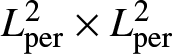 $L^2_{\rm per} \times L^2_{\rm per}$ consists of eigenvalues
 $\lambda$ of finite algebraic multiplicity. If
 $\lambda \in \mathbb{C}$ is an eigenvalue, so are
 $\bar{\lambda}$,
 $-\lambda$ and
 $-\bar{\lambda}$.
Proof. The first assertion holds since  $\mathbb{T}$ is compact,
 $\mathcal{K}$ and
 $\mathcal{L}$ are unbounded operators in
 $L^2_{\rm per}$, and
 $\mathcal{H}$,
 $\mathcal{M}$ and
 $\mathcal{M}^*$ are bounded operators in
 $L^2_{\rm per}$. The second assertion follows from the properties:
•
 $\mathcal{K}$,
$\mathcal{L}$,
$\mathcal{M}$,
$\mathcal{M}^*$ and
$\mathcal{H}$ have real-valued coefficients.
•
$\mathcal{K}$,
$\mathcal{L}$,
$\mathcal{M}$ and
$\mathcal{M}^*$ are invariant and
$\mathcal{H}$ is covariant with respect to the parity transformation
$(\Pi f)(x) = f(-x)$ such that
\begin{equation*}
\Pi \mathcal{H} \Pi = -\mathcal{H}, \quad \Pi \mathcal{M} \Pi = \mathcal{M}, \quad \Pi \mathcal{M}^* \Pi = \mathcal{M}^*, \quad \Pi \mathcal{L} \Pi = \mathcal{L}, \quad
\Pi \mathcal{K} \Pi = \mathcal{K}.
\end{equation*}




As a consequence of these properties, if  $(v,w) \in H^1_{\rm per} \times H^1_{\rm per}$ is an eigenfunction of the spectral problem (1.19) for an eigenvalue
 $\lambda \in \mathbb{C}$, then
 $(\bar{v},\bar{w})$ is an eigenfunction for
 $\bar{\lambda}$,
 $(\Pi v, -\Pi w)$ is an eigenfunction for
 $-\lambda$ and
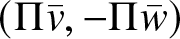 $(\Pi \bar{v}, -\Pi \bar{w})$ is an eigenfunction for
 $-\bar{\lambda}$.
Remark 1. The nonlinear system (1.10) and the linearized system (1.16) admit a Hamiltonian formulation with a nonlocal symplectic structure. Since we study the spectral stability of travelling waves, we will not write the Hamiltonian structure explicitly.
To introduce the modulational stability problem, we extend the spectral stability problem (1.19) from co-periodic perturbations  $(v,w) \in H^1_{\rm per} \times H^1_{\rm per}$ to perturbations defined on the real line
 $(v,w) \in H^1(\mathbb{R}) \times H^1(\mathbb{R})$. To do so, we use the Floquet–Bloch theory and introduce the characteristic exponent
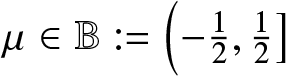 $\mu \in \mathbb{B} := \left(-\frac{1}{2},\frac{1}{2} \right]$, where
 $\mathbb{B}$ is reciprocal to
 $\mathbb{T} = [0,2\pi)$. By using the Bloch transform
 \begin{equation*}
v(u) = \int_{\mathbb{B}} \hat{v}(u,\mu) e^{i \mu u} d \mu, \quad
w(u) = \int_{\mathbb{B}} \hat{w}(u,\mu) e^{i \mu u} d \mu,
\end{equation*}
where  $(\hat{v},\hat{w})(\cdot,\mu) \in H^1_{\rm per} \times H^1_{\rm per}$ for every fixed
 $\mu \in \mathbb{B}$, we obtain
 \begin{equation}
\left\{\begin{array}{ll}
\mathcal{K}_{\mu} \hat{w} &= \lambda \mathcal{M}_{\mu} \hat{v}, \\
\mathcal{L}_{\mu} \hat{v} &= \lambda (\mathcal{M}^*_{\mu} \hat{w}
- 2 c \mathcal{H}_{\mu} \hat{v}),
\end{array}
\right.
\end{equation}
which is again defined in the periodic domain  $\mathbb{T}$ for every
 $\mu \in \mathbb{B}$. The expressions for each operator
 $\mathcal{K}_{\mu}$,
 $\mathcal{L}_{\mu} $,
 $\mathcal{M}_{\mu} $,
 $\mathcal{M}^*_{\mu} $ and
 $\mathcal{H}_{\mu}$ are obtained below for
 $\mu \neq 0$.
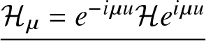 $\underline{\mathcal{H}_{\mu} = e^{-i \mu u} \mathcal{H} e^{i \mu u}}$: Since
 $\mathcal{H} \sum\limits_{n \in \mathbb{Z}} \hat{f}_n e^{i (\mu + n) u}
= i \sum\limits_{n \in \mathbb{Z}} {\rm sgn}(\mu + n) \hat{f}_n e^{i (\mu + n) u}$ and
 $\mu \in \mathbb{B}$, we get
 \begin{equation*}
\mathcal{H}_{\mu} f = \mathcal{H} f + i {\rm sgn}(\mu) \hat{f}_0, \quad \mu \neq 0,
\end{equation*}
where  $\hat{f}_0 = \langle 1, f \rangle$ due to normalization of the inner product in
 $L^2_{\rm per}$. Thus, we can define
 \begin{equation}
\mathcal{H}_{\pm} = \mathcal{H} \pm i \langle 1, \cdot \rangle, \quad \pm \mu \gt 0,
\end{equation}
where  $\mathcal{H}$ is defined by (1.2).
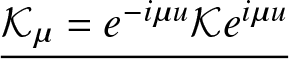 $\underline{\mathcal{K}_{\mu} = e^{-i \mu u} \mathcal{K} e^{i \mu u}}$: Since
 $\mathcal{K}_{\mu} = - \mathcal{H}_{\mu} (\partial_u + i \mu)$, we get the expansion
 \begin{equation}
\mathcal{K}_{\mu} = \mathcal{K} - i \mu \mathcal{H}_{\pm}, \quad \pm \mu \gt 0,
\end{equation}
where  $\mathcal{K}$ is defined by (1.3).
 $\underline{\mathcal{M}_{\mu} = e^{-i \mu u} \mathcal{M} e^{i \mu u}}$: It follows from (1.17) and (1.21) that
 $\mathcal{M}_{\mu} = \mathcal{M}_{\pm}$ given by
 \begin{equation}
\mathcal{M}_{\pm} = 1 + \mathcal{K}\eta + \eta' \mathcal{H}_{\pm}, \quad \pm \mu \gt 0.
\end{equation}
Similarly, we get 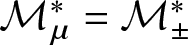 $\mathcal{M}^*_{\mu} = \mathcal{M}^*_{\pm}$ given by
 \begin{equation}
\mathcal{M}^*_{\pm} = 1 + \mathcal{K}\eta - \mathcal{H}_{\pm}(\eta' \; \cdot), \quad \pm \mu \gt 0.
\end{equation}
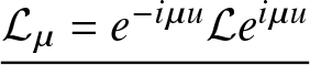 $\underline{\mathcal{L}_{\mu} = e^{-i \mu u} \mathcal{L} e^{i \mu u}}$: It follows from (1.18) and (1.22) that
 \begin{equation}
\mathcal{L}_{\mu} = \mathcal{L} - i \mu \mathcal{L}_{\pm}, \quad \pm \mu \gt 0,
\end{equation}
where
 \begin{equation}
\mathcal{L}_{\pm} = c^2 \mathcal{H}_{\pm} - \eta \mathcal{H}_{\pm} - \mathcal{H}_{\pm} (\eta \; \cdot).
\end{equation}
As a result of (1.21), (1.22), (1.23), (1.24) and (1.25), we can rewrite the stability problem (1.20) in the equivalent form
 \begin{equation}
\left\{\begin{array}{ll}
(\mathcal{K} - i \mu \mathcal{H}_{\pm}) \hat{w} &= \lambda \mathcal{M}_{\pm} \hat{v}, \\
(\mathcal{L} - i \mu \mathcal{L}_{\pm}) \hat{v} &= \lambda (\mathcal{M}^*_{\pm} \hat{w}
- 2 c \mathcal{H}_{\pm} \hat{v}),
\end{array}
\right.
\end{equation}
where  $\mu \neq 0$ and the two signs refer to
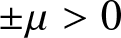 $\pm \mu \gt 0$. The following result extends Lemma 1 to the stability problem (1.27).
Lemma 2. The spectrum of the spectral problem (1.27) in 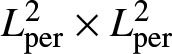 $L^2_{\rm per} \times L^2_{\rm per}$ consists of eigenvalues
 $\lambda$ of finite algebraic multiplicity for each fixed
 $\mu \in \mathbb{B}$. Consequently, we can enumerate the spectral bands of the stability spectrum in
 $L^2(\mathbb{R}) \times L^2(\mathbb{R})$ as
 \begin{equation}
\sigma_S = \cup_{j \in \mathbb{N}} \{\lambda_j(\mu), \;\; \mu \in \mathbb{B} \}.
\end{equation}
If  $\lambda_j(\mu)$ is a spectral band of the spectral stability problem (1.27) for
 $\mu \in \mathbb{B}$, so are
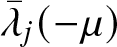 $\bar{\lambda}_j(-\mu)$,
 $-\lambda_j(-\mu)$ and
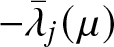 $-\bar{\lambda}_j(\mu)$.
Proof. The first assertion holds again because  $\mathbb{T}$ is compact,
 $\mathcal{K}$ and
 $\mathcal{L}$ are unbounded operators in
 $L^2_{\rm per}$, whereas
 $\mathcal{H}_{\pm}$,
 $\mathcal{M}_{\pm}$,
 $\mathcal{M}^*_{\pm}$ and
 $\mathcal{L}_{\pm}$ are bounded operators in
 $L^2_{\rm per}$. The second assertion follows from the properties of
 $\mathcal{K}$,
 $\mathcal{L}$,
 $\mathcal{M}$,
 $\mathcal{M}^*$ and
 $\mathcal{H}$ in the proof of Lemma 1 and the additional properties
 \begin{equation*}
\mathcal{H}_{\pm} = \overline{\mathcal{H}}_{\mp}, \quad \mathcal{H}_{\pm} |_{\mu \to -\mu} = \mathcal{H}_{\mp}, \quad
\Pi \mathcal{H}_{\pm} \Pi = -\mathcal{H}_{\mp},
\end{equation*}
Consequently, if  $(\hat{v}(\mu),\hat{w}(\mu)) \in H^1_{\rm per} \times H^1_{\rm per}$ is an eigenfunction of the spectral problem (1.27) for an eigenvalue
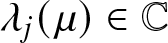 $\lambda_j(\mu) \in \mathbb{C}$ with fixed
 $\mu \in \mathbb{B}$, then
 $(\bar{v}(-\mu),\bar{w}(-\mu))$ is an eigenfunction for
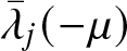 $\bar{\lambda}_j(-\mu)$,
 $(\Pi v(-\mu), -\Pi w(-\mu))$ is an eigenfunction for
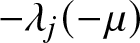 $-\lambda_j(-\mu)$ and
 $(\Pi \bar{v}(\mu), -\Pi \bar{w}(\mu)$ is an eigenfunction for
 $-\bar{\lambda}_j(\mu)$.
Remark 2. We say that the periodic wave with the profile 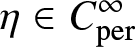 $\eta \in C^{\infty}_{\rm per}$ is modulationally unstable if the spectral bands in
 $\sigma_S$ intersecting the origin do not coincide with a subset of
 $i\mathbb{R}$ for
 $\lambda \neq 0$.
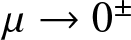
Remark 3. The original spectral problem (1.20) is not analytic at  $\mu = 0$ due to the different behaviour of the linear operators
 $\mathcal{K}_{\mu}$,
 $\mathcal{L}_{\mu}$,
 $\mathcal{M}_{\mu}$,
 $\mathcal{M}_{\mu}^*$ and
 $\mathcal{H}_{\mu}$ in the limit
 $\mu \to 0^{\pm}$. However, after extending
 $\mathcal{K}_{\mu}$,
 $\mathcal{L}_{\mu}$,
 $\mathcal{M}_{\mu}$,
 $\mathcal{M}_{\mu}^*$ and
 $\mathcal{H}_{\mu}$ differently for
 $\mu \gt 0$ and
 $\mu \lt 0$, the reformulated spectral problem (1.27) is now analytic in
 $\mu$ and
 $\lambda$ for both signs.
1.3. Main results and organization of the paper
Figure 1 shows numerical approximations of the spectral bands (1.28) when the travelling wave is continued with respect to the steepness parameter  $s$ defined in (1.15) from the small-amplitude limit given by (1.13)–(1.14) towards the limiting wave with the peaked profile. We observe four bifurcations of the spectral bands near the origin described below. These four bifurcations were discovered in [Reference Deconinck, Dyachenko and Semenova17], see their Figure 3. Based on the first three cycles, it was conjectured in [Reference Deconinck, Dyachenko and Semenova17] that the four bifurcations are repeated recurrently in the same sequence infinitely many times before the wave profile becomes peaked.
Remark 4. Panels (h) and (l) are repeated twice in Figure 1 to show that between (a)–(h), (h)–(l) and (l)–(o), we recalibrate the scales along the real and imaginary axis of the complex  $\lambda$-plane, for better presentation of bifurcations. The scaling units are explicitly shown in the first panel of the calibration and are kept for all subsequent panels until the next calibration.
Our main results consist of the derivation and justification of the criteria and the normal forms for the four bifurcations near the origin shown in Figure 1. To be precise, we describe each bifurcation separately in the list below.
• The first figure-
$8$ bands are seen in (a). This bifurcation, also known as the Benjamin–Feir instability, is studied in Appendix A. The normal form for the stability bands is given by
(1.29)where\begin{equation}
\left( \lambda - \frac{i \mu}{2} \right)^2 = \frac{1}{64} \mu^2 (8 a^2 - \mu^2) + \mathcal{O}(a^6 + \mu^6),
\end{equation}
$a \in \mathbb{R}$ is a small parameter of the asymptotic expansions (1.13) and (1.14). The normal form was derived and justified in the previous works [Reference Berti, Maspero and Ventura6, Reference Creedon and Deconinck14].• Panels (b)–(d) show the second bifurcation, for which the slopes of the figure-
$8$ bands become vertical at
$\lambda = 0$, after which the figure-
$8$ bands break into two instability bubbles along the imaginary axis. This bifurcation is analysed in Section 4 by expanding solutions of the spectral problem (1.27) near
$(\mu,\lambda) = (0,0)$. The normal form for the stability bands is given by
(1.30)\begin{equation}
\mathcal{P}'(c_0) \left( \lambda - \frac{i \mu \mathcal{N}'(c)}{2 \mathcal{P}'(c)} \right)^2 + \frac{\mu^2 \Delta'(c_0) (c - c_0)}{4 \mathcal{P}'(c_0)} + \mathcal{D} |\mu|^3 = \mathcal{O}(\mu^4),
\end{equation}Figure 1.Transformation of the spectral bands in the modulational stability problem (1.27) when the steepness parameter
$s$ of Stokes waves is increased.1 Long description
The composite shows plots arranged in a four-column grid, labeled a through o, each displaying spectral band curves plotted in the complex plane. The horizontal axis of each plot represents the real part of the spectral parameter and the vertical axis represents the imaginary part. The steepness parameter of Stokes waves increases progressively from panel a toward panel o, moving left to right and top to bottom across the grid. In panel a, the scale markers show 0.2 on the vertical axis and 0.05 on the horizontal axis. Two small closed loops are stacked vertically along the imaginary axis, forming a narrow vertically oriented figure-eight shape centered near the origin. In panel b, the two loops expand significantly, each becoming a large symmetric teardrop-shaped lobe, one above and one below the origin, still joined at the center. In panel c, the two lobes grow wider and more rounded, maintaining the symmetric hourglass arrangement along the vertical axis. In panel d, the upper lobe becomes triangular with a flattened top, while the lower lobe remains more rounded and the junction at the origin remains a crossing point. In panel e, the two lobes collapse into two thin nearly horizontal elliptical rings, one above and one below the origin, separated along the imaginary axis. In panel f, the elliptical rings shrink further and flatten into near-horizontal dash-like segments at two positions along the imaginary axis. In panel g, the segments remain as narrow horizontal marks at two symmetric positions along the imaginary axis, with very small extent along the real axis. In panel h, shown twice in the grid to mark a scale recalibration, the scale markers show 0.2 on the vertical axis and 0.2 on the horizontal axis. A single wide horizontal elliptical loop appears, centered near the origin and extending broadly along the real axis. In the repeated panel h in the third row, the loop is clearly visible with the recalibrated scale. In panel i, the wide horizontal ellipse narrows slightly but retains its elongated horizontal orientation. In panel j, the ellipse continues to narrow and becomes a more symmetric oval shape oriented horizontally. In panel k, the oval splits at the center, forming a horizontal figure-eight with two lobes extending to the left and right of the origin along the real axis. In panel l, shown twice to mark another scale recalibration, the scale markers show 0.02 on the vertical axis and 0.002 on the horizontal axis. The two lobes separate into two distinct small ovals positioned symmetrically to the left and right of the vertical axis. In panel m, the two separated ovals remain distinct and symmetric about the vertical axis. In panel n, the two ovals reconnect at the origin, forming a small vertically oriented figure-eight shape. In panel o, the figure-eight grows slightly larger and more rounded, with the two lobes now clearly defined above and below the origin. Some curves appear as dotted segments in panels h and l, indicating regions of the spectrum rendered differently from the solid curve segments in other panels.
closed with the consistency condition
$c - c_0 = \mathcal{O}(\mu)$, where
$\mathcal{P}(c)$ and
$\mathcal{N}(c)$ are given by (2.5) and (2.7),
$\Delta(c)$ is the bifurcation parameter given by (2.10),
$\mathcal{D}$ is the numerical coefficient given by (4.40), and
$c_0$ is a simple root of
$\Delta(c)$. See Theorems 1 and 2. This bifurcation originates from the tangential intersection of the double-degenerate spectral bands at
$(\mu,\lambda) = (0,0)$. It has not been considered in the previous literature.• Panels (e)–(g) show the third bifurcation, for which a new circular instability bubble emerges near
$\lambda = 0$. This bifurcation is analysed in Section 5 by expanding solutions of the spectral problem (1.27) near
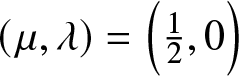
$(\mu,\lambda) = \left(\frac{1}{2},0\right)$. The normal form for the stability bands is given by
(1.31)closed with the consistency condition\begin{equation}
\lambda^2\mathcal{A}_{1} + 2 i c_0 \tilde{\mu} \lambda \mathcal{A}_{2} + \tilde{\mu}^2 \mathcal{A}_{3}
- \Lambda'(c_0) (c-c_0) \| \psi_0 \|^2_{L^2} = \mathcal{O}\left( |\tilde{\mu}|^3 \right),
\end{equation}
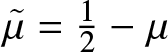
$c - c_0 = \mathcal{O}(\tilde{\mu}^2)$, where
$\tilde{\mu} = \frac{1}{2} - \mu$,
$\mathcal{A}_{1,2,3}$ are numerical coefficients given by (5.10),
$\Lambda(c)$ is the simple eigenvalue of
associated with the eigenfunction
\begin{equation*}
\mathcal{L}_{\rm aper} : H^1_{\rm aper} \subset L^2_{\rm aper} \to L^2_{\rm aper},
\end{equation*}
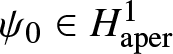
$\psi_0 \in H^1_{\rm aper}$, and
$c_0$ is a simple root of
$\Lambda(c)$. See Theorems 3 and 4. This bifurcation originates from the one-dimensional kernel of
$\mathcal{L}_{\rm aper}$ in the space of double-periodic (antiperiodic) perturbations. Such subharmonic bifurcations for fixed rational values of
$\mu$, including
$\mu = \frac{1}{2}$, have been studied in [Reference Buffoni, Dancer and Toland11].• Panels (j)–(l) show the fourth bifurcation, for which the instability band surrounding
$\lambda = 0$ reconnects into the figure-
$\infty$ bands, which then break into two instability bubbles along the real axis. This bifurcation is analysed in Section 6 by expanding solutions of the spectral problem (1.27) near
$(\mu,\lambda) = (0,0)$. The normal form for the stability bands is given by
(1.32)closed with the consistency condition\begin{equation}
\lambda^4 \mathcal{B} - i \mu \lambda \mathcal{N}'(c_0) + \lambda^2 \mathcal{P}''(c_0) (c - c_0) = \mathcal{O}(\mu^2),
\end{equation}
$c - c_0 = \mathcal{O}(|\mu|^{2/3})$, where
$\mathcal{P}(c)$ and
$\mathcal{N}(c)$ are given by (2.5) and (2.7),
$\mathcal{B}$ is the numerical coefficient given by (6.14), and
$c_0$ is a simple root of
$\mathcal{P}'(c)$. See Theorem 5. This bifurcation originates from the extreme points of energy
$\mathcal{H}$ (equivalently, the horizontal momentum
$\mathcal{P}$), at which the spectral stability problem (1.19) for co-periodic perturbations admits the zero-eigenvalue bifurcation. The zero-eigenvalue bifurcation has been studied in [Reference Dyachenko and Pelinovsky20].• Panels (m)–(o) show the first bifurcation again, for which new figure-
$8$ bands arise near
$\lambda = 0$. This bifurcation is analysed in Section 7 by expanding solutions of the spectral problem (1.27) near
$(\mu,\lambda) = (0,0)$. The normal form for the stability bands is given by
(1.33)closed with the consistency condition\begin{equation}
\left( \lambda - \frac{i \mu c_0}{2} \right)^2 = \mu^2 \left[ \mathcal{N}(c_0) - \frac{5c_0}{4} \mathcal{P}(c_0) \right]
\left[ |\mu| + \frac{\delta_0 \varepsilon}{c_0^2 \langle 1, v_0 \rangle} \right] + \mathcal{O}(|\mu|^{7/2}),
\end{equation}
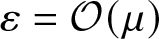
$c^2 = c_0^2 + \delta_0 \varepsilon^2 + \mathcal{O}(\varepsilon^3)$ and
$\varepsilon = \mathcal{O}(\mu)$, where
$\mathcal{P}(c)$ and
$\mathcal{N}(c)$ are given by (2.5) and (2.7),
$\delta_0$ is given by (7.26) and
$c_0$ is the fold bifurcation point, for which the kernel of
in the space of co-periodic perturbations is two-dimensional with the eigenfunctions of opposite parity
\begin{equation*}
\mathcal{L} : H^1_{\rm per} \subset L^2_{\rm per} \to L^2_{\rm per}
\end{equation*}
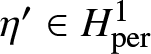
$\eta' \in H^1_{\rm per}$ and
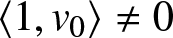
$v_0 \in H^1_{\rm per}$ satisfying
$\langle 1, v_0 \rangle \neq 0$. See Theorems 6 and 7. This bifurcation originates from the extreme points of speed
$c$, at which the family of smooth travelling waves parameterized by steepness
$s$ has a fold bifurcation with respect to the speed
$c$. Fold bifurcations have been studied in [Reference Buffoni, Dancer and Toland11].

























Remark 5. It is remarkable that the normal form (1.33) for the steep Stokes waves is different from the normal form (1.29) for the small-amplitude Stokes waves, despite both describing a figure-8 bifurcation. It is seen from (1.30) and (1.33) that the original spectral problem (1.20) is not analytic at  $\mu = 0$ because the pseudo-differential operators
 $\mathcal{H}_{\mu}$ and
 $\mathcal{K}_{\mu}$ are singular at
 $\mu = 0$. Nevertheless, we derive the normal forms by analytic extension of these operators for
 $\mu \gt 0$ and
 $\mu \lt 0$ in the reformulated spectral problem (1.27).
The numerical method used in our computations is described in Appendix B. The travelling wave profile 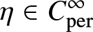 $\eta \in C^{\infty}_{\rm per}$ is computed from Babenko’s equation (1.11) as a function of the wave steepness
 $s$, see Appendix B.1. The spectral bands (1.28) are computed from the stability problem (1.27) for each steepness
 $s$ as functions of the Floquet parameter
 $\mu$, see Appendix B.2. We compare the spectral bands computed from the normal form equations for each bifurcation described above with the spectral bands zoomed near the origin in the complex
 $\lambda$-plane. Table 1 provides numerical data for the steepness
 $s$, speed
 $c$ and energy
 $\mathcal{H}$ at each bifurcation point in the first two cycles of the four bifurcations.
Parameters of Stokes waves at the four bifurcation points: steepness  $s$, speed
 $c$, energy
 $\mathcal{H}$ and the bifurcation type in the first two cycles

Table 1 Long description
Five columns record steepness, speed, energy, bifurcation type, and a cross reference. Eight rows follow. The first is a baseline carrying steepness 0, speed 1 and energy 0. Across the remaining rows steepness climbs steadily from about 0.109 to 0.141, while speed rises from about 1.061 to a peak near 1.093 and then eases very slightly. Energy climbs from about 0.346 to a maximum near 0.465 in the fourth row, then declines gently through the last four rows. Bifurcation types cycle through four named profile shapes, a figure eight, an hourglass, an ellipse and a lemniscate, each appearing twice, once in a first cycle and once in a second. Steepness and speed are given to eight decimal places and energy to eleven, so the closely spaced later rows differ only in their trailing digits.
The main computations of the normal forms are described in Sections 4–7. Section 2 contains two preliminary results about integral characteristics of the travelling waves with profile 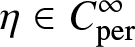 $\eta \in C^{\infty}_{\rm per}$ and about the behaviour of the spectral problem (1.27) in the limit
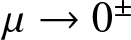 $\mu \to 0^{\pm}$. Section 3 describes the Newton polytope method, which is used to justify the balance of asymptotic terms in the direct Puiseux expansions.
2. Preliminary results
We describe two results which clarify the behaviour of the spectral problem (1.27) near  $(\mu,\lambda) = (0,0)$. Section 2.1 discusses smoothness of continuation of the travelling wave with the even profile
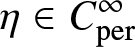 $\eta \in C^{\infty}_{\rm per}$ with respect to the wave speed
 $c \in (1,c_*)$ and derives some relations between the integral quantities related to the horizontal momentum (1.6) and the energy (1.8). Both facts are useful in the explicit computations of the projection matrix at
 $(\mu,\lambda) = (0,0)$ used in the bifurcation theory of Sections 4, 6 and 7. Section 2.2 compares the limit
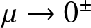 $\mu \to 0^{\pm}$ in the spectral problem (1.27) with the co-periodic stability problem (1.19), where we prove that the eigenfunctions of the two different spectral problems are related by an invertible transformation.
2.1. Integral quantities for travelling waves
Recall the linear operator
 \begin{equation*}
\mathcal{L} : H^1_{\rm per} \subset L^2_{\rm per} \to L^2_{\rm per},
\end{equation*}
given by (1.18). It represents a linearization of Babenko’s equation (1.11) at the travelling wave with the even profile 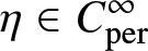 $\eta \in C^{\infty}_{\rm per}$. Due to the translational symmetry, we have
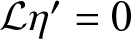 $\mathcal{L} \eta' = 0$ with the odd eigenfunction
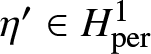 $\eta' \in H^1_{\rm per}$. Also recall the linear operator
 \begin{equation*}
\mathcal{K} : H^1_{\rm per} \subset L^2_{\rm per} \to L^2_{\rm per},
\end{equation*}
given by (1.3). By using Fourier series, we have  $\mathcal{K} 1 = 0$ with the even eigenfunction
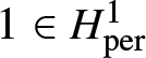 $1 \in H^1_{\rm per}$. Furthermore, we obtain the following relations by explicit computations:
 \begin{equation}
\mathcal{L} 1 = -\left(1 + 2 \mathcal{K} \eta\right),
\end{equation}
 \begin{equation}
\mathcal{L} \eta = \eta - c^2 \mathcal{K} \eta,
\end{equation}
and
 \begin{equation}
\mathcal{L}_{\pm} \eta' = -c^2 \mathcal{K} \eta + \eta \mathcal{K}\eta + \frac{1}{2} \mathcal{K}\eta^2 = -\eta,
\end{equation}
where  $\mathcal{L}_{\pm} : L^2_{\rm per} \to L^2_{\rm per}$ is given by (1.26).
The following lemma gives a sufficient condition for differentiability of the mapping  $c \to \eta \in C^{\infty}_{\rm per}$ at any
 $c \in (1,c_*)$.
Lemma 3. If  ${\rm Ker}(\mathcal{L}) = {\rm span}(\eta')$, then the mapping
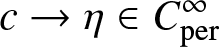 $c \to \eta \in C^{\infty}_{\rm per}$ is continuously differentiable for this value of
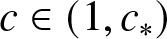 $c \in (1,c_*)$ and
 \begin{equation}
\mathcal{L} \partial_c \eta = - 2 c \mathcal{K} \eta.
\end{equation}
Proof. If  $\eta$ is even, then
 $\eta'$ is odd. Restricting solutions to Babenko’s equation (1.11) to even functions is allowed since
 $\mathcal{K}$ is parity-preserving in the subspace of
 $H^1_{\rm per}$ spanned by even functions, which we denote by
 $H^1_{\rm per,e}$. The linearized operator
 $\mathcal{L}$ acting on
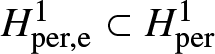 $H^1_{\rm per,e} \subset H^1_{\rm per}$ has a trivial kernel and its spectrum consists of eigenvalues which do not accumulate to
 $0$, see [Reference Buffoni, Dancer and Toland10, Reference Buffoni, Dancer and Toland11]. Hence, by the implicit function theorem for
 $(\eta,c) \in H^1_{\rm per,e} \times \mathbb{R}$, there exists a
 $C^1$ continuation of the solution
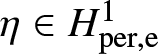 $\eta \in H^1_{\rm per,e}$ to Babenko’s equation (1.11) in
 $c$ for this value of
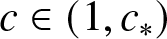 $c \in (1,c_*)$. By differentiating (1.11) in
 $c$, we obtain (2.4), where
 $\mathcal{K} \eta \perp {\rm Ker}(\mathcal{L})$ with the unique solution
 $\partial_c \eta \in H^1_{\rm per,e}$.
Remark 6. We say that the profile 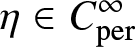 $\eta \in C^{\infty}_{\rm per}$ is at the fold bifurcation if
 ${\rm Ker}(\mathcal{L}) \neq {\rm span}(\eta')$ for this value of
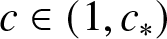 $c \in (1,c_*)$. The fold bifurcation is included in our study in Section 7. Bifurcations in Sections 4–6 hold away from the fold bifurcation when
 ${\rm Ker}(\mathcal{L}) = {\rm span}(\eta')$.
Related to the travelling wave profile 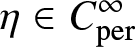 $\eta \in C^{\infty}_{\rm per}$ we define the wave momentum
 $\mathcal{P}(c)$ and the wave energy
 $\mathcal{H}(c)$ by evaluating
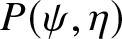 $P(\psi,\eta)$ and
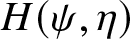 $H(\psi,\eta)$ in (1.6) and (1.8) at
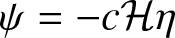 $\psi= -c \mathcal{H} \eta$:
 \begin{equation}
\mathcal{P}(c) = c \langle K \eta, \eta \rangle
\end{equation}
and
 \begin{equation}
\mathcal{H}(c) = \frac{c^2}{2} \langle K \eta, \eta \rangle + \frac{1}{2}\langle \eta^2, (1+K\eta) \rangle.
\end{equation}
In addition, we introduce the squared  $L^2$ norm, which is a part of the energy (2.6) but is not a conservative quantity in the time evolution of the system (1.4):
 \begin{equation}
\mathcal{N}(c) := \langle \eta, \eta \rangle.
\end{equation}
These integral quantities are used in the Taylor expansion of solutions of the spectral problem (1.27) near  $(\mu,\lambda) = (0,0)$. Some useful relations are derived in the following lemma.
Lemma 4. It follows that
 \begin{equation}
\mathcal{H}(c) = \frac{5}{6} c\mathcal{P}(c) + \frac{1}{6}\mathcal{N}(c),
\end{equation}
where  $\mathcal{P}(c)$,
 $\mathcal{H}(c)$, and
 $\mathcal{N}(c)$ are defined by (2.5), (2.6) and (2.7). If
 ${\rm Ker}(\mathcal{L}) = {\rm span}(\eta')$, then we also have
 \begin{equation}
\mathcal{H}'(c) = c\mathcal{P'}(c) = \mathcal{N}'(c) + 5\mathcal{P}(c).
\end{equation}
Proof. It follows from (1.11) that
 \begin{align*}
c \mathcal{P}(c) - \mathcal{N}(c) = \langle (c^2 \mathcal{K}\eta - \eta), \eta \rangle = \frac{3}{2} \langle \eta^2, \mathcal{K} \eta \rangle.
\end{align*}
Eliminating  $\langle \eta^2, \mathcal{K} \eta \rangle$ from
 \begin{equation*}
2 \mathcal{H}(c) = c \mathcal{P}(c) + \mathcal{N}(c) + \langle \eta^2, \mathcal{K} \eta \rangle,
\end{equation*}
we obtain (2.8).
To derive (2.9) under the assumption  ${\rm Ker}(\mathcal{L}) = {\rm span}(\eta')$, see Lemma 3, we obtain from (1.12) that
 \begin{equation*}
\Lambda_c(\eta) = c \mathcal{P}(c) - \mathcal{H}(c).
\end{equation*}
Differentiating  $\Lambda_c(\eta)$ in
 $c$ and using (1.11), yields
 $\frac{d}{dc} \Lambda_c(\eta) = \mathcal{P}(c)$, which implies the first identity in (2.9). For the second identity in (2.9), we obtain
 \begin{align*}
c\mathcal{P}'(c) - \mathcal{N}'(c) &= c\langle \mathcal{K}\eta, \eta \rangle +
2 \langle (c^2 \mathcal{K} \eta - \eta), \partial_c \eta \rangle \\
&= \mathcal{P}(c) - 2 \langle \mathcal{L} \eta, \partial_c \eta \rangle \\
&= \mathcal{P}(c) + 4 c \langle \mathcal{K} \eta, \eta \rangle \\
&= 5\mathcal{P}(c),
\end{align*}
where we have used (2.2), (2.4) and self-adjointness of  $\mathcal{L}$ in
 $L^2_{\rm per}$.
Remark 7. Let  $\sigma_0$ be the smallest eigenvalue of
 $\mathcal{L} : H^1_{\rm per} \subset L^2_{\rm per} \to L^2_{\rm per}$. Then, it follows from (2.2) that
 \begin{align*}
1 - \frac{c\mathcal{P}(c)}{\mathcal{N}(c)} = \frac{\langle \mathcal{L} \eta, \eta \rangle}{\langle \eta, \eta \rangle} \geq \sigma_0.
\end{align*}
Since it follows from (2.1) that  $\langle \mathcal{L} 1, 1 \rangle = -1 \lt 0$, we have
 $\sigma_0 \lt 0$, which implies that
 \begin{equation*}
c \mathcal{P}(c) \leq (1 - \sigma_0) \mathcal{N}(c).
\end{equation*}
Remark 8. By using the second identity in (2.9), we obtain
 \begin{align}\Delta(c) &= 4 \mathcal{P}'(c) \mathcal{N}(c) - c \mathcal{P}'(c) \mathcal{N}'(c) + [\mathcal{N}'(c)]^2 \notag \\
&= 4 \mathcal{P}'(c) \mathcal{N}(c) - 5 \mathcal{P}(c) \mathcal{N}'(c),\end{align}
where  $\Delta(c)$ appears in Section 4, see the proof of Theorem 1.
Figure 2 displays the numerically computed values of  $\mathcal{H}'(c)$ defined by (2.9) (red solid line) and
 $\Delta(c)$ defined by (2.10) (green solid line) as functions of the steepness parameter
 $s$ on a logarithmic scale. The vertical lines mark zeros of
 $c'(s)$, for which the mapping
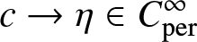 $c \to \eta \in C^{\infty}_{\rm per}$ is not continuously differentiable in
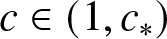 $c \in (1,c_*)$. Zeros of
 $\Delta(c)$ (green line) mark the hourglass bifurcation, see Section 4. Zeros of
 $\mathcal{H}'(c)$ (red line) mark the figure-
 $\infty$ bifurcation, see Section 6. Zeros of
 $c'(s)$ (vertical lines) mark the figure-
 $8$ bifurcation, see Section 7. The recurrent structure of zeros of
 $\Delta(c)$,
 $\mathcal{H}'(c)$ and
 $c'(s)$ is obvious from the plots.
The dependence of  $\mathcal{H}'(c)$ (red solid) and
 $\Delta(c)$ (green solid) versus the wave steepness
 $s$, with the vertical lines for zeros of
 $c'(s)$.

In our numerical computations, we compute  $\mathcal{P}(c)$,
 $\mathcal{P}'(c)$,
 $\mathcal{H}(c)$ and
 $\mathcal{H}'(c)$, after which we obtain
 $\mathcal{N}(c)$ and
 $\mathcal{N}'(c)$ from the relations (2.8) and (2.9). The values of
 $\mathcal{P}(c)$ and
 $\mathcal{H}(c)$ are obtained from (2.5) and (2.6), The derivative
 $\mathcal{P}'(c)$ is obtained from
 \begin{align*}
\mathcal{P}'(c) = \langle \mathcal{K}\eta, \eta \rangle + 2c\langle \mathcal{K}\partial_c\eta, \eta \rangle,
\end{align*}
where  $\partial_c\eta$ is determined from solving the linear equation (2.4) numerically via the MINRES method to a prescribed tolerance defined as
 \begin{equation*}
\frac{\|\mathcal{L}\partial_c\eta + 2c\mathcal{K}\eta \|_{L^2}}{
\|2c\mathcal{K}\eta \|_{L^2}} \leq 10^{-10}.
\end{equation*}
From  $\mathcal{P}'(c)$, we obtain the derivative
 $\mathcal{H}'(c) = c \mathcal{P}'(c)$ by using (2.9).
Figure 3 displays the first (smallest) eigenvalues of the operator  $\mathcal{L}$ for co-periodic (green curves) and anti-periodic (red curves) perturbations versus the normalized steepness. In the limit of zero steepness, we obtain from (1.13) and (1.14):
 \begin{equation*}
\lim_{a \to 0} \mathcal{L} = \mathcal{K}-1.
\end{equation*}
Therefore, we have a simple eigenvalue at  $-1$ and a sequence of double eigenvalues at
 $\{0,1,2,\dots \}$ for co-periodic perturbations associated with the Fourier modes
 $1$ and
 $e^{\pm i n u}$ for
 $n \in \mathbb{N}$, respectively, and a sequence of double eigenvalues
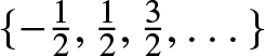 $\{-\frac{1}{2}, \frac{1}{2}, \frac{3}{2}, \dots \}$ for anti-periodic perturbations associated with the Fourier modes
 $e^{\pm \frac{i}{2} (2n-1) u}$ for
 $n \in \mathbb{N}$. These eigenvalues are continued with respect to the steepness parameter.
The red solid dots correspond to the subharmonic (double-period) bifurcation of travelling wave solutions, which results in the ellipse bifurcation in the stability problem (1.27) described in Section 5. The green solid dots correspond to the turning points of the speed  $c$ versus steepness
 $s$, where
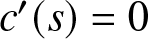 $c'(s) = 0$, see vertical lines on Figure 2. At these points, the mapping
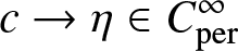 $c \to \eta \in C^{\infty}_{\rm per}$ is not continuously differentiable, see Lemma 3, and the figure-
 $8$ bifurcation occurs in the spectral problem (1.27) described in Section 7. Each zero crossing for the red curve occurs between zero crossings by the green curve.
The dependence of the first (smallest) eigenvalues of  $\mathcal{L}$ for co-periodic (green) and anti-periodic (red) perturbations.

Figure 3 Long description
The horizontal axis label reads, s lim minus s over s lim. The horizontal axis uses a logarithmic scale with tick labels 1, 10 superscript minus 1, 10 superscript minus 2 and 10 superscript minus 3. The vertical axis has tick labels 2, 1, 0, minus 1 and minus 2 and represents eigenvalues. A dotted horizontal reference line is drawn at eigenvalue 0. Multiple smooth line branches are plotted across the full horizontal range. Several branches remain above 0 for the full range, several branches cross the 0 reference line and several branches extend below 0 toward minus 2. Five filled circular markers lie on the eigenvalue 0 line at the horizontal tick positions 1, 10 superscript minus 1, 10 superscript minus 2, a point between 10 superscript minus 2 and 10 superscript minus 3 and 10 superscript minus 3.
2.2. The limit
$\mu \to 0^{\pm}$ in the stability problem (1.27)
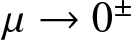
It is obvious that the limit  $\mu \to 0^{\pm}$ in the spectral problem (1.27) is different from the co-periodic stability problem (1.19) because of the jumps in the continuation of the linear operators
 $\mathcal{H}$,
 $\mathcal{M}$ and
 $\mathcal{M}^*$ for
 $\mu \neq 0$. However, the following lemma shows that eigenfunctions of (1.27) in the limit
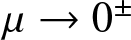 $\mu \to 0^{\pm}$ are related to eigenfunctions of (1.19) by using a simple invertible transformation.
Lemma 5. Let  $(v,w) \in H^1_{\rm per} \times H^1_{\rm per}$ be an eigenfunction of (1.19) for an eigenvalue
 $\lambda \in \mathbb{C} \backslash \{0\}$. Then, the eigenfunction
 $(\hat{v},\hat{w}) \in H^1_{\rm per} \times H^1_{\rm per}$ of (1.27) in the limit
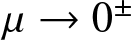 $\mu \to 0^{\pm}$ exists for the same eigenvalue
 $\lambda \in \mathbb{C} \backslash \{0\}$ and is given by
 \begin{equation}
\hat{v} = \mp i \langle 1, v \rangle \eta' + v, \qquad
\hat{w} = \pm i c \langle 1, v \rangle + w.
\end{equation}
Proof. In the limit 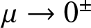 $\mu \to 0^{\pm}$, we rewrite (1.27) in the explicit form:
 \begin{equation}
\left\{\begin{array}{ll}
\mathcal{K} \hat{w} &= \lambda \left( \mathcal{M} \hat{v} \pm i \langle 1, \hat{v} \rangle \eta' \right), \\
\mathcal{L} \hat{v} &= \lambda \left( \mathcal{M}^* \hat{w}
- 2 c \mathcal{H} \hat{v} \mp i \langle \eta', \hat{w} \rangle \mp 2 c i \langle 1, \hat{v} \rangle \right).
\end{array}
\right.
\end{equation}
Since  $\mathcal{K}1 = 0$ and
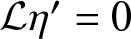 $\mathcal{L} \eta' = 0$, we have the following orthogonality condition for every solution
 $(\hat{v},\hat{w}) \in H^1_{\rm per} \times H^1_{\rm per}$ of (2.12) with
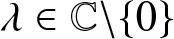 $\lambda \in \mathbb{C} \backslash \{0\}$:
 \begin{equation}
\left. \begin{array}{r}
\langle (1 + 2 \mathcal{K} \eta), \hat{v} \rangle = 0, \\
\langle \eta', \hat{w} \rangle - 2 c \langle \mathcal{K} \eta, \hat{v} \rangle = 0,
\end{array}
\right\}
\end{equation}
where we have used  $\mathcal{M}^* 1 = 1 + 2 \mathcal{K} \eta$ and
 $\mathcal{M} \eta' = \eta'$ obtained from (1.17). The two constraints imply
 $\langle \eta', \hat{w} \rangle + c \langle 1, \hat{v} \rangle = 0$, which enables us to rewrite (2.12) in the equivalent form:
 \begin{equation}
\left\{\begin{array}{ll}
\mathcal{K} \hat{w} &= \lambda \left( \mathcal{M} \hat{v} \pm i \langle 1, \hat{v} \rangle \eta' \right), \\
\mathcal{L} \hat{v} &= \lambda \left( \mathcal{M}^* \hat{w}
- 2 c \mathcal{H} \hat{v} \mp c i \langle 1, \hat{v} \rangle \right).
\end{array}
\right.
\end{equation}
By using the transformation (2.11), we obtain  $\mathcal{K} \hat{w} = \mathcal{K} w$,
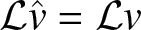 $\mathcal{L} \hat{v} = \mathcal{L} v$ and
 $\langle 1, \hat{v} \rangle = \langle 1, v \rangle$. Furthermore, the inhomogeneous terms in (2.14) cancel out under the transformation (2.11) and the spectral problem (2.14) becomes equivalent to (1.19) for
 $(v,w) \in H^1_{\rm per} \times H^1_{\rm per}$.
Remark 9. Due to Lemma 5, the algebraic and geometric multiplicities of every eigenvalue of the co-periodic spectral problem (1.19) are equal to those of the spectral problem (1.27) as 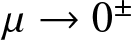 $\mu \to 0^{\pm}$, that is, of the spectral problem (2.12). The result holds for
 $\lambda = 0$ due to the orthogonality conditions (2.13) needed for generalized eigenfunctions.
3. Methodology
We explain the method that we use for the justification analysis of the four bifurcations considered in Sections 4–7. The spectral bands (1.28) are defined by the eigenvalues  $\lambda$ of the spectral problem (1.27) continued as functions of the Floquet parameter
 $\mu$. In particular, we are interested in the behaviour of these functions near the origin for
 $\mu$ being close to either
 $0$ or
 $\frac{1}{2}$, and we recover the behaviour of the spectral bands seen in Figure 1 from the normal forms justified via some rigorous theory.
If we investigate zeros of some Fredholm determinant which give eigenvalues of the purely discrete spectrum of the spectral problem (1.27) for a finite  $\mu \in \mathbb{B}$, we can use the Weierstrass preparation theorem to pull out the (finite) part that is vanishing, and ignore the rest [Reference Hormander26]. This is somewhat standard, though it technically requires some analyticity to use. The spectral problem (1.27) is analytic in
 $\mu$ and
 $\lambda$ for both signs, see Remark 3, and the analytic projections to the discrete spectrum near
 $\lambda = 0$ are justified.
To explain ideas of the justification analysis, we study eigenvalues and eigenvectors of a matrix perturbed by a small parameter  $\varepsilon$. This parameter represents either small
 $|\mu|$ in Sections 4, 6 and 7 or
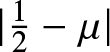 $|\frac{1}{2} - \mu|$ in Section 5. Furthermore, the small deviation of the speed
 $c$ from the critical value
 $c_0$ for the four bifurcations also produces perturbation terms, which are represented by another small parameter. In what follows, we require the second small parameter to be scaled consistently with the parameter
 $\varepsilon$ in order to obtain splittings of degenerate eigenvalues near
 $\lambda = 0$ at the leading order of the asymptotic theory.
3.1. Two double Jordan blocks
This situation represents the bifurcation studied in Section 4. For simplicity, we take the following normalized matrix
 \begin{equation}
A_0 = \begin{pmatrix} 0 & 1 & 0 & 0 \\ 0 & 0 & 0 &0 \\ 0 & 0 & 0& 1 \\ 0 & 0 & 0 &0 \end{pmatrix}
\end{equation}
with a quadruple zero eigenvalue. We want to consider how the eigenvalues of
 \begin{equation*}
A(\varepsilon) = A_0 + \varepsilon B + \varepsilon^2 C
\end{equation*}
unfold for  $\varepsilon \neq 0$, where
 $B$ and
 $C$ are some given generic matrices with entries
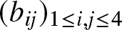 $(b_{ij})_{1 \leq i,j \leq 4}$ and
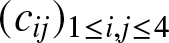 $(c_{ij})_{1 \leq i,j \leq 4}$.
We first explain the method of direct Puiseux expansions, which is used in Section 4 (and other sections). Then, we justify the direct method by using the Newton polytope method for analysis of the characteristic polynomials. The advantage of the direct Puiseux expansions is that they avoid computations of all projections of perturbations to the basis of generalized eigenfunctions and single out only the perturbation terms which lead to splitting of eigenvalues near  $\lambda = 0$.
Direct Puiseux expansions. We fix the standard basis  $\{e_1,e_2,e_3,e_4\}$ such that
 \begin{equation*}
A_0 e_1 = 0, \quad A_0 e_2 = e_1, \quad A_0 e_3 = 0, \quad A_0 e_4 = e_3.
\end{equation*}
Because of the Jordan block structure of  $A_0$, the small eigenvalues of
 $A(\varepsilon)$ scale like
 $\mathcal{O}(\varepsilon^{1/2})$ as
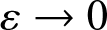 $\varepsilon \to 0$ [Reference Hinch25]. This theory allows us to use Puiseux expansions for eigenvalues
 \begin{equation*}
\lambda(\varepsilon) = \varepsilon^{1/2} \lambda_1 + \varepsilon \lambda_2 + \mathcal{O}(\varepsilon^{3/2})
\end{equation*}
and eigenvectors
 \begin{equation*}
v = v_0 + \varepsilon^{1/2} v_1 + \varepsilon v_2 + \mathcal{O}(\varepsilon^{3/2}),
\end{equation*}
which are inserted into the matrix eigenvalue problem  $A(\varepsilon) v = \lambda(\varepsilon) v$. Collecting powers of
 $\varepsilon^{1/2}$, we get the following results.
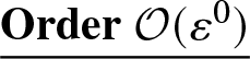 $\underline{\boldsymbol{\mathrm{Order}} \ \mathcal{O}(\varepsilon^0)}$: Since
 \begin{equation*}
A_0 v_0 = 0 \quad \Rightarrow \quad v_0 \in \ker A_0 = \mathrm{span}\left\{e_1,e_3\right\},
\end{equation*}
we can write
 \begin{equation}
v_0 = \alpha e_1 + \beta e_3,
\end{equation}
with coefficients 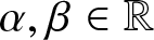 $\alpha, \beta \in \mathbb{R}$.
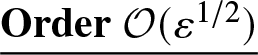 $\underline{\boldsymbol{\mathrm{Order}} \ \mathcal{O}(\varepsilon^{1/2})}$: Since
 \begin{equation*}
A_0 v_1 = \lambda_1 v_0 \quad \Rightarrow \quad
v_1 \in \ker A_0^2 = \mathrm{span}\left\{e_1,e_2,e_3,e_4\right\}.
\end{equation*}
we can write
 \begin{equation}
v_1 = \lambda_1 (\alpha e_2 + \beta e_4) + u_1,
\end{equation}
where  $u_1 \in \ker{A_0}$ is arbitrary. Since
 $\alpha,\beta$ are arbitrary in (3.2), we can set
 $u_1 \equiv 0$ without loss of generality.
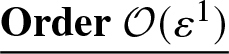 $\underline{\boldsymbol{\mathrm{Order}} \ \mathcal{O}(\varepsilon^{1})}$: We obtain
 \begin{equation*}
A_0 v_2 + B v_0 = \lambda_1 v_1 + \lambda_2 v_0.
\end{equation*}
The Fredholm alternative theorem implies that there exists a solution for  $v_2$ if and only if
 \begin{equation}
\lambda_1 v_1 - B v_0 \in {\rm ran}(A_0) = [\ker(A_0^T)]^{\perp},
\end{equation}
since  $\lambda_2 v_0 \in {\rm ran}(A_0)$. Using (3.2), (3.3) and
 $\langle e_{2,4}, e_{1,3} \rangle = 0$ (this is essentially the reason why we can set
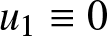 $u_1 \equiv 0$), we get from (3.4) due to
 $\ker(A_0^T) = \mathrm{span}\left\{e_2,e_4\right\}$,
 \begin{equation}
\left\{\begin{array}{l}
(b_{21} \alpha + b_{23} \beta ) = \lambda_1^2 \alpha, \\
(b_{41} \alpha + b_{43} \beta) = \lambda_1^2 \beta.
\end{array} \right.
\end{equation}
A non-trivial pair  $(\alpha,\beta)$ exists in (3.5) if and only if
 $\lambda_1^2$ is an eigenvalue of the projection matrix
 \begin{equation}
G_1 = \begin{pmatrix} b_{21} & b_{23} \\ b_{41} & b_{43} \end{pmatrix} = \begin{pmatrix} \langle e_2, B e_1\rangle & \langle e_2, B e_3\rangle \\ \langle e_4, B e_1\rangle& \langle e_4, B e_3\rangle \end{pmatrix}.
\end{equation}
 $G_1$ provides a map for the image of
 $B$ acting on the right eigenspace
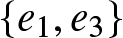 $\{e_1, e_3\}$, projected onto the left eigenspace
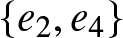 $\{e_2, e_4\}$. If we denote the eigenvalues of
 $G_1$ by
 $s_1$ and
 $s_2$, then the four eigenvalues
 $\lambda(\varepsilon)$ of
 $A(\varepsilon)$ split from the quadruple zero eigenvalue if
 $\varepsilon \neq 0$ according to the following asymptotic balance:
 \begin{equation}
\left\{\begin{array}{l}
\lambda(\varepsilon) = \varepsilon^{1/2} \sqrt{s_1} + \mathcal{O}(\varepsilon), \\
\lambda(\varepsilon) = -\varepsilon^{1/2}\sqrt{s_1} + \mathcal{O}(\varepsilon), \\
\lambda(\varepsilon) = \varepsilon^{1/2}\sqrt{s_2} + \mathcal{O}(\varepsilon), \\
\lambda(\varepsilon) = -\varepsilon^{1/2}\sqrt{s_2} + \mathcal{O}(\varepsilon).
\end{array} \right.
\end{equation}
For each of these eigenvalues, we have an associated eigenvector  $v_0$ in (3.2) and an associated generalized eigenvector
 $v_1$ in (3.3). Furthermore, we can find the second-order correction
 $v_2$ by
 \begin{equation}
v_2 = A_0^T(\lambda_1 v_1 - B v_0) + \lambda_2 (\alpha e_2 + \beta e_4) + u_2
\end{equation}
where  $u_2 \in \ker{A_0}$ is arbitrary.
For the splitting of the quadruple zero eigenvalue in Section 4, we have a simplification compared to the general theory. Namely, the projection matrix  $G_1$ in (3.6) has
 \begin{equation}
b_{21} = b_{23} = b_{41} = 0, \quad b_{43} \neq 0,
\end{equation}
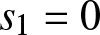
see (4.6). As a result, 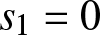 $s_1 = 0$ and
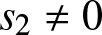 $s_2 \neq 0$ in (3.7) so that only two of the four eigenvalues
 $\lambda(\varepsilon)$ of
 $A(\varepsilon)$ split at the order of
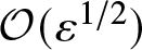 $\mathcal{O}(\varepsilon^{1/2})$, whereas the other two eigenvalues split at the higher order of
 $\mathcal{O}(\varepsilon)$.
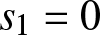
To consider the higher-order splitting of the eigenvalue  $\lambda(\varepsilon) = \mathcal{O}(\varepsilon)$ for
 $s_1 = 0$ and
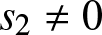 $s_2 \neq 0$, we introduce the eigenvector of
 $G_1$ for the zero eigenvalue
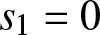 $s_1 = 0$ as
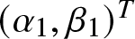 $(\alpha_1, \beta_1)^T$:
 \begin{equation*}
G_1 \begin{pmatrix} \alpha_1 \\ \beta_1 \end{pmatrix} = 0.
\end{equation*}
This yields  $v_0$ in (3.2) and since
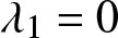 $\lambda_1 = 0$ and
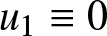 $u_1 \equiv 0$, then (3.3) implies that
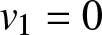 $v_1 = 0$. Furthermore, (3.8) implies that
 \begin{equation}
v_2 = - A_0^T B v_0 + \lambda_2 (\alpha_1 e_2 + \beta_1 e_4) + u_2,
\end{equation}
where  $u_2 \in \ker{A_0}$. Unlike previously, we need to assume here that
 $u_2 \neq 0$ since we get constraints on
 $u_2$ from (3.11) below; hence, we write
 $u_2 = \gamma e_1 + \delta e_3$ with new coefficients
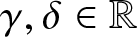 $\gamma,\delta \in \mathbb{R}$.
 $\underline{\boldsymbol{\mathrm{Order}} \ \mathcal{O}(\varepsilon^{3/2})}$ We obtain
 \begin{equation*}
A_0 v_3 = \lambda_3 v_0 \quad \Rightarrow \quad
v_3 = \lambda_3(\alpha_1 e_2 + \beta_1 e_4)
+ u_3,
\end{equation*}
where  $u_3 \in \ker{A_0}$ is arbitrary.
 $\underline{\boldsymbol{\mathrm{Order}} \ \mathcal{O}(\varepsilon^{2})}$: We obtain
 \begin{equation*}
A_0 v_4 + B v_2 + C v_0 = \lambda_2 v_2 + \lambda_4 v_0.
\end{equation*}
The Fredholm alternative theorem implies that there exists a solution for  $v_4$ if and only if
 \begin{equation*}
\lambda_2 v_2 - B v_2 - C v_0 \in {\rm ran}(A_0) = [\ker(A_0^T)]^{\perp}.
\end{equation*}
Substituting  $v_2$ from (3.10) and using the fact that
 $\ker{A_0^T} = \mathrm{span}\left\{e_2,e_4\right\}$ we arrive at the pair of conditions:
 \begin{equation}
\lambda_2^2 \begin{pmatrix} \alpha_1 \\ \beta_1 \end{pmatrix} - \lambda_2 G_2 \begin{pmatrix} \alpha_1 \\ \beta_1 \end{pmatrix} - G_3 \begin{pmatrix} \alpha_1 \\ \beta_1 \end{pmatrix} = G_1 \begin{pmatrix} \gamma \\ \delta \end{pmatrix},
\end{equation}
where
 \begin{equation*}
G_2 = \begin{pmatrix} \langle e_2, (A_0^T B + B A_0^T) e_1\rangle & \langle e_2, (A_0^T B + B A_0^T) e_3\rangle \\ \langle e_4, (A_0^T B + B A_0^T) e_1\rangle& \langle e_4,(A_0^T B + B A_0^T) e_3\rangle \end{pmatrix}
\end{equation*}
and
 \begin{equation*}
G_3 = \begin{pmatrix} \langle e_2, (B A_0^{T} B - C) e_1\rangle & \langle e_2, (B A_0^{T} B - C) e_3\rangle \\ \langle e_4, (B A_0^{T} B - C) e_1\rangle& \langle e_4, (B A_0^{T} B - C) e_3\rangle \end{pmatrix}.
\end{equation*}
The left-hand side of (3.11) is a pair of polynomials in  $\lambda_2$, dependent on the eigenvector
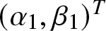 $(\alpha_1,\beta_1)^T$ of the zero eigenvalue of
 $G_1$, which we can denote as
 $(p_1(\lambda_2),p_2(\lambda_2))^T$. There exists a solution of (3.11) for
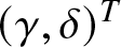 $(\gamma,\delta)^T$ if and only if
 $(p_1(\lambda_2),p_2(\lambda_2))^T$ is in the range of
 $G_1$, i.e., orthogonal to a eigenvector of
 $G_1^T$ for the zero eigenvalue
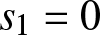 $s_1 = 0$, denoted by
 $(\ell_1,\ell_2)^T$:
 \begin{equation}
\ell_1 p_1(\lambda_2) + \ell_2 p_2(\lambda_2) = 0.
\end{equation}
This gives a quadratic equation on  $\lambda_2$ with two roots labelled as
 $\lambda_2^{\pm}$. Combined with the other pair related to
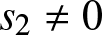 $s_2 \neq 0$, see (3.7), we obtain four eigenvalues splitting from the quadruple zero eigenvalue if
 $\varepsilon \neq 0$ according to the following asymptotic balance:
 \begin{equation}
\left\{\begin{array}{l}
\lambda(\varepsilon) = \varepsilon \lambda_2^+ + \mathcal{O}(\varepsilon^{3/2}), \\
\lambda(\varepsilon) = \varepsilon \lambda_2^- + \mathcal{O}(\varepsilon^{3/2}), \\
\lambda(\varepsilon) = \varepsilon^{1/2}\sqrt{s_2} + \mathcal{O}(\varepsilon), \\
\lambda(\varepsilon) = -\varepsilon^{1/2}\sqrt{s_2} + \mathcal{O}(\varepsilon).
\end{array} \right.
\end{equation}
For the case (3.9), the eigenvector of  $G_1$ in (3.6) for
 $s_1 = 0$ is
 $(\alpha_1,\beta_1)^T = (1,0)^T$ so that the second equation in the system (3.11) defines uniquely
 $\delta$, whereas the first equation in the system (3.11) gives a quadratic equation on
 $\lambda_2$, which is equivalent to (3.12). The correction
 $\gamma$ is not uniquely defined and can be set to
 $0$.
Justification with the Newton polytope method. A suitable algorithm which justifies the direct expansions leading to the splitting formulas (3.7) or (3.13) is based on the Newton polytope method for the characteristic polynomials [Reference Kirwan28]. Let 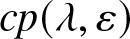 $cp(\lambda,\varepsilon)$ denote the characteristic polynomial of the perturbed matrix
 $A(\varepsilon)$:
 \begin{equation*}
cp(\lambda,\varepsilon) := \det\left(A_0 + \varepsilon B + \varepsilon^2 C - \lambda I \right).
\end{equation*}
The polynomial 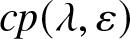 $cp(\lambda,\varepsilon)$ is a polynomial in two variables
 $\lambda$ and
 $\varepsilon$. Since we are looking at perturbations near zero, we can get a leading approximation of this polynomial via the lower convex hull of its Newton polytope in the
 $(\lambda,\varepsilon)$ lattice, where points correspond to integer powers [Reference Kirwan28]. That is, we expand
 $cp(\lambda,\varepsilon)$ in powers of
 $\lambda$ and
 $\varepsilon$ and keep track of the non-zero coefficient in front of powers. For each of the powers
 $\lambda^i\varepsilon^j$ with a non-zero coefficient, we depict solid points on an integer lattice
 $(i,j)$. Then we take the lower-convex hull of these points.
Figure 4 represents the generic case for the matrix  $A_0$ in (3.1), for which we have
 \begin{equation}
cp(\lambda,\varepsilon) = \lambda^4 + a_1 \varepsilon\lambda^2 + a_2 \varepsilon^2 + h.o.t.,
\end{equation}
where  $h.o.t.$ denotes terms of the order of
 $\varepsilon \lambda^3$,
 $\varepsilon^2 \lambda^2$,
 $\varepsilon^2 \lambda$ and
 $\varepsilon^3$. When the coefficients
 $a_1$ and
 $a_2$ are nonzero, the lower-convex hull with the boundary connecting
 $(0,2)$,
 $(2,1)$ and
 $(4,0)$ gives the lowest-order approximation to the characteristic polynomial.
The Newton polytope of  $cp(\lambda,\varepsilon) = \det\left(A_0 + \varepsilon B + \varepsilon^2 C - \lambda I \right)$ given by (3.14). The boundary of the lower convex hull consists of the lattice points at
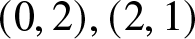 $(0,2),(2,1)$ and
 $(4,0)$.

The coefficients  $a_1$ and
 $a_2$ are given in terms of the entries of
 $B$. In certain cases [Reference Ma and Edelman37, Reference Moro, Burke and Overton38] some formulas are known to exist, though not for the general forms of the matrices. However, in our examples, the dimensions are low enough that we can write out the characteristic polynomial and collect terms explicitly. In particular, for the matrix
 $A_0$ in (3.1) perturbed by
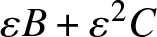 $\varepsilon B + \varepsilon^2 C$, we can write
 \begin{equation*}
\begin{cases}
a_1 = -(b_{21} + b_{43}) = -\mathrm{Tr}\left(G_1\right), \\
a_2 = b_{21}b_{43} - b_{23}b_{41} = \det(G_1),
\end{cases}
\end{equation*}
in agreement with our previous direct computations, see (3.5). Substituting 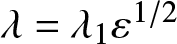 $\lambda = \lambda_1 \varepsilon^{1/2}$ into (3.14) yields
 \begin{equation*}
cp(\varepsilon^{1/2} \lambda_1, \varepsilon) = \varepsilon^2 \left( \lambda_1^4 - \mathrm{Tr}\left(G_1\right) \lambda_1^2 + \det(G_1) \right) + \mathcal{O}(\varepsilon^{ \gt 2})
\end{equation*}
from which we obtain 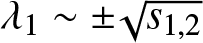 $\lambda_1 \sim \pm \sqrt{s_{1,2}}$, where
 $s_1$ and
 $s_2$ are eigenvalues of
 $G_1$, and recover the eigenvalue splitting in (3.7).
If we now assume that  $s_1 = 0$ and
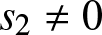 $s_2 \neq 0$, then
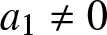 $a_1 \neq 0$ and
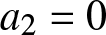 $a_2 = 0$, so that we remove the point
 $(0,2)$ in the lower convex hull and re-compute the approximating polynomial. The characteristic polynomial is now expanded as
 \begin{equation}
cp(\lambda,\varepsilon) = \lambda^4 + a_1 \varepsilon \lambda^2 +a_3 \varepsilon^2 \lambda + a_4 \varepsilon^3 + h.o.t.,
\end{equation}
where  $a_1 = -\mathrm{Tr}\left(G_1\right)$ as before,
 $a_3$ and
 $a_4$ have been computed with the symbolic software,
 \begin{equation*}
\begin{cases}
a_3 = (b_{11}+b_{22})\,b_{43}-b_{41}(b_{13}+b_{24})
-b_{23}(b_{31}+b_{42})
+ b_{21}(b_{33}+b_{44}), \\
a_4 = b_{41}(b_{13} b_{22} + b_{24} b_{33} - c_{23}) -b_{43}(b_{11} b_{22} + b_{24} b_{31} - c_{21}) \\
\quad \quad
+ b_{23}(b_{11} b_{42} + b_{31} b_{44} - c_{41})
- b_{21}(b_{13} b_{42} + b_{33} b_{44} - c_{43}),
\end{cases}
\end{equation*}
and  $h.o.t.$ denote terms of the order of
 $\varepsilon \lambda^3$,
 $\varepsilon^2 \lambda^2$,
 $\varepsilon^3 \lambda$ and
 $\varepsilon^4$.
Figure 5 shows the lower-convex hull of the Newton polytope if  $a_1, a_3, a_4 \neq 0$. In this case, we have two slopes, so there will be two branches of the eigenvalues. The first is again found by setting
 $\lambda = \lambda_1 \varepsilon^{1/2}$ which corresponds to the slope
 $-\frac{1}{2}$ connecting
 $(2,1)$ and
 $(4,0)$ in Figure 5. Substituting this into (3.15), we have
 \begin{equation*}
cp(\varepsilon^{1/2} \lambda_1,\varepsilon) = \varepsilon^2\left(\lambda_1^4 + a_1 \lambda_1^2\right) + \mathcal{O}(\varepsilon^{ \gt 2}),
\end{equation*}
which recovers the first non-zero correction 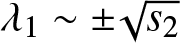 $\lambda_1 \sim \pm \sqrt{s_2}$ for the non-zero eigenvalue of the matrix
 $G_1$. There are also two eigenvalues that are
 $0$ here, indicating that the slope
 $-\frac{1}{2}$ cannot see the eigenvalue splitting at this level. We next make the substitution
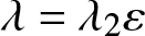 $\lambda = \lambda_2 \varepsilon$, which corresponds to the slope
 $-1$ connecting
 $(0,3)$ and
 $(2,1)$ in Figure 5, and we arrive at
 \begin{align*}
cp(\varepsilon \lambda_2, \varepsilon) &= \varepsilon^4 \lambda_2^4 + \varepsilon^3 \left( a_1 \lambda_2^2 + a_3 \lambda_2 + a_4 \right) + h.o.t \\
&= \varepsilon^3 \left( a_1 \lambda_2^2 + a_3 \lambda_2 + a_4 \right) + \mathcal{O}(\varepsilon^{ \gt 3}).
\end{align*}
The Newton polytope of  $cp(\lambda,\varepsilon) = \det\left(A_0 + \varepsilon B + \varepsilon^2 C - \lambda I \right)$ given by (3.15). The boundary of the lower convex hull consists of the lattice points at
 $(0,3),(1,2), (2,1)$ and
 $(4,0)$.

This recovers the quadratic equation
 \begin{equation*}
a_1 \lambda_2^2 + a_3 \lambda_2 + a_4 =0,
\end{equation*}
which is equivalent to (3.12). By denoting the two roots of the quadratic equation by  $\lambda_2^{\pm}$ and combining with the previous case, we have recovered the eigenvalue splitting in (3.13). The eigenvalue splitting as in (3.13) is obtained with direct Puiseux expansions, see (4.7) with (4.20) and (4.22) with (4.26) in Section 4.
3.2. One double Jordan block
This situation represents the bifurcation studied in Section 5 and corresponds to the following normalized matrix
 \begin{equation*}
A_0 = \begin{pmatrix} 0 & 1 \\ 0 & 0 \end{pmatrix}
\end{equation*}
with a double zero eigenvalue. Since this case is much simpler than the previous case of two double Jordan blocks, the eigenvalue splitting is obtained from the quadratic characteristic polynomial by using simpler computations, which we do not write here. We only point out that  $G_1 = 0$ (where
 $G_1$ is a scalar) so that the double zero eigenvalue splits as
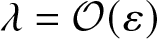 $\lambda = \mathcal{O}(\varepsilon)$ instead of
 $\lambda = \mathcal{O}(\varepsilon^{1/2})$, see (5.3) with (5.9) in Section 5.
3.3. One quadruple and one double Jordan blocks
This situation represents the bifurcation studied in Section 6 and corresponds to the following normalized matrix
 \begin{equation}
A_0 = \begin{pmatrix} 0 & 1 & 0 & 0 & 0 & 0 \\ 0 & 0 & 1 & 0 & 0 & 0 \\0 & 0 & 0 & 1 & 0 & 0 \\ 0 & 0 & 0 & 0 & 0 & 0 \\ 0 & 0 & 0 & 0 & 0 & 1 \\ 0 & 0 & 0 & 0 & 0 & 0 \end{pmatrix}
\end{equation}
with the zero eigenvalue of algebraic multiplicity  $6$. The characteristic polynomial is expanded as
 \begin{equation}
cp(\lambda, \varepsilon) = \lambda^6 + a_1 \varepsilon \lambda^2 + a_2 \varepsilon^2 + h.o.t,
\end{equation}
where
 \begin{equation*}
\begin{cases}
a_1 = - b_{41}, \\
a_2 = b_{41} b_{65} - b_{45} b_{61} = \det \begin{pmatrix} b_{41} & b_{61} \\ b_{45} & b_{65} \end{pmatrix}.
\end{cases}
\end{equation*}
Figure 6 shows the lower convex hull of the Newton polytope for the characteristic polynomial (3.17) with the boundary consisting of two lines if 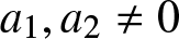 $a_1, a_2 \neq 0$. Taking into account the two slopes
 $-\frac{1}{4}$ and
 $-\frac{1}{2}$ of the lower boundary, we can get four eigenvalues by using the scaling
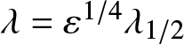 $\lambda = \varepsilon^{1/4} \lambda_{1/2}$ and two eigenvalues by using the scaling
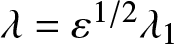 $\lambda = \varepsilon^{1/2} \lambda_1$ with the leading-order approximations given by
 \begin{equation}
\lambda_{1/2} \sim e^{2k \pi/4} \sqrt[4]{-a_1} \quad k = 1,2,3,4 \quad \quad \textrm{and} \quad \quad \lambda_1 \sim \pm \sqrt{-a_2/a_1},
\end{equation}
respectively. However, our case of study corresponds to 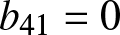 $b_{41} = 0$, which is the same coefficient as
 $b_{21}$ in (3.6), see (3.9). Therefore, we need to consider the case of
 $a_1 = 0$, for which the eigenvalue splitting (3.18) is not applicable.
The Newton polytope of  $cp(\lambda,\varepsilon) = \det\left(A_0 + \varepsilon B + \varepsilon^2 C - \lambda I \right)$ given by (3.17). The boundary of the lower convex hull consists of the lattice points at
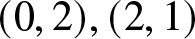 $(0,2),(2,1)$ and
 $(6,0)$.

If 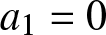 $a_1 = 0$, then the characteristic polynomial is expanded as
 \begin{equation}
cp(\lambda, \varepsilon) = \lambda^6 + a_3 \lambda^3 \varepsilon + a_2 \varepsilon^2 + h.o.t.,
\end{equation}
where  $a_2 = - b_{45} b_{61}$ as before and
 $a_3 = -b_{31}-b_{42}$. Figure 7 shows the lower convex hull of the Newton polytope for the characteristic polynomial (3.19) with the boundary given by a single line. This suggests that the six eigenvalues have the correct scaling
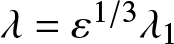 $\lambda = \varepsilon^{1/3} \lambda_1$, with the leading-order approximation for
 $\lambda_1$ given by
 \begin{equation}
\lambda_1 \sim \frac{e^{2 \pi i k/3}}{2} \left( -a_3 \pm \sqrt{a_3^2 - 4 a_2} \right) \quad k = 1, 2,3.
\end{equation}
The Newton polytope of  $cp(\lambda,\varepsilon) = \det\left(A_0 + \varepsilon B + \varepsilon^2 C - \lambda I \right)$ given by (3.19). The boundary of the lower convex hull consists of the lattice points at
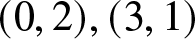 $(0,2),(3,1)$ and
 $(6,0)$.

However, our case of study corresponds to 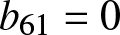 $b_{61} = 0$, which is the same coefficient as
 $b_{41}$ in (3.6), see (3.9). Therefore, we need to consider the double-degenerate case of
 $a_1 = a_2 = 0$, for which the eigenvalue splitting (3.20) is not applicable.
If  $a_1 = a_2 = 0$, then the characteristic polynomial is expanded as
 \begin{equation}
cp(\lambda, \varepsilon) = \lambda_1^6 + a_3 \varepsilon \lambda^3 + a_4 \varepsilon^2 \lambda + a_5 \varepsilon^3 + h.o.t.,
\end{equation}
where  $a_3 = -b_{31} - b_{42}$ as before and
 $a_4$,
 $a_5$ are obtained with the symbolic software:
 \begin{equation*}
\begin{cases}
a_4 = (-b_{35} - b_{46})\, b_{61}
+ b_{45}\,(-b_{51} - b_{62})
+ (b_{31} + b_{42})\, b_{65}\\
a_5 = b_{65}\Big(
- b_{11} b_{42} - b_{21} b_{43} - b_{31} b_{44}
- b_{46} b_{51} + c_{41}
\Big) \\
\qquad
+ b_{61}\Big(
b_{15} b_{42} + b_{25} b_{43} + b_{35} b_{44}
+ b_{46} b_{55} - c_{45}
\Big) \\
\qquad
+ b_{45}\Big(
b_{11} b_{62} + b_{21} b_{63} + b_{31} b_{64}
+ b_{51} b_{66} - c_{61}
\Big).
\end{cases}
\end{equation*}
Figure 8 shows the lower convex hull of the Newton polytope for the characteristic polynomial (3.21) with the boundary given by three lines. This suggests three different scalings for the six eigenvalues, with the leading-order approximation given by
 \begin{equation}
\lambda \sim \varepsilon^{1/3} e^{2 \pi i k/3} \sqrt[3]{-a_3} \quad k = 1,2,3 \quad \textrm{and } \quad \lambda \sim \pm \varepsilon^{1/2} \sqrt{-\frac{a_4}{a_3}} \quad \textrm{and} \quad \lambda \sim - \varepsilon \frac{a_5}{a_4}.
\end{equation}
The Newton polytope of  $cp(\lambda,\varepsilon) = \det\left(A_0 + \varepsilon B + \varepsilon^2 C - \lambda I \right)$ given by (3.21). The boundary of the lower convex hull consists of the lattice points at
 $(0,3),(1,2),(3,1)$ and
 $(6,0)$.

The eigenvalue splitting as in (3.22) is obtained with direct Puiseux expansions, see (6.1) with (6.15) in Section 6.
3.4. Two simple and one double Jordan blocks
This situation represents the bifurcation studied in Section 7 and corresponds to the following normalized matrix
 \begin{equation}
A_0 = \begin{pmatrix} 0 & 0 & 0 & 0 \\ 0 & 0 & 0 & 0 \\ 0 & 0 & 0 & 1 \\ 0 & 0 & 0 & 0 \end{pmatrix}
\end{equation}
with the quadruple zero eigenvalue. The characteristic polynomial is expanded as
 \begin{equation}
cp(\lambda;\varepsilon) = \lambda^4 + a_1 \varepsilon \lambda^2 + a_2 \varepsilon^2 \lambda + a_3 \varepsilon^3 + h.o.t.,
\end{equation}
where
 \begin{equation*}
\begin{cases}
a_1 = - b_{43} \\
a_2 = b_{43}(b_{11} + b_{22}) - b_{13}b_{41} - b_{23}b_{42} \\
a_3 = b_{13} b_{22} b_{41}
- b_{12} b_{23} b_{41}
- b_{13} b_{21} b_{42}
+ b_{11} b_{23} b_{42}
+ b_{12} b_{21} b_{43}
- b_{11} b_{22} b_{43},
\end{cases}
\end{equation*}
from which
 \begin{equation*}
a_3 = - \det\begin{pmatrix}
b_{11} & b_{12} & b_{13}\\
b_{21} & b_{22} & b_{23}\\
b_{41} & b_{42} & b_{43}\\
\end{pmatrix}.
\end{equation*}
The lower convex hull of the Newton polytope for the characteristic polynomial (3.24) is identical to the one shown in Figure 5 if  $a_1, a_2, a_3 \neq 0$. The boundary consists of two lines. For the line with the slope
 $-\frac{1}{2}$, we set
 $\lambda = \lambda_1 \varepsilon^{1/2}$ and substitute into (3.24) to get
 \begin{equation*}
cp(\varepsilon^{1/2} \lambda_1, \varepsilon) = \varepsilon^2 \lambda_1^2( \lambda_1^2 + a_1) + \mathcal{O}(\varepsilon^{ \gt 2}),
\end{equation*}
which defines two roots 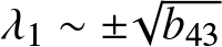 $\lambda_1 \sim \pm \sqrt{b_{43}}$. For the line with the slope
 $-1$, we set
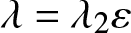 $\lambda = \lambda_2 \varepsilon$ and substitute into (3.24) to get
 \begin{equation*}
cp(\varepsilon \lambda_2, \varepsilon) = \varepsilon^3( a_1 \lambda_2^2 + a_2 \lambda_2 + a_3) + \mathcal{O}(\varepsilon^{ \gt 3}),
\end{equation*}
which defines two roots near the two roots of  $a_1 \lambda_2^2+ a_2 \lambda_2 + a_3 = 0$. Denoting these two roots by
 $\lambda_2^{\pm}$ and combining with the previous case, we obtain the eigenvalue splitting given by
 \begin{equation}
\lambda \sim \pm \varepsilon^{1/2} \sqrt{b_{43}} \quad \textrm{and } \quad \lambda \sim \varepsilon \lambda_2^{\pm}.
\end{equation}
In our case of study in Section 7, we have  $a_1 = -b_{43} \neq 0$, see (3.9). However, we also have
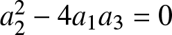 $a_2^2 - 4 a_1 a_3 = 0$ so that
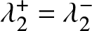 $\lambda_2^+ = \lambda_2^-$ is a double root of
 $a_1 \lambda_2^2+ a_2 \lambda_2 + a_3 = 0$, see (7.8) and (7.9). As a result, there exists a degeneracy in the eigenvalue splitting as in (3.25) at the order of
 $\mathcal{O}(\varepsilon)$.
To unfold the degeneracy of the double root, we look at the next terms in the expansion of the characteristic polynomial 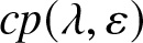 $cp(\lambda,\varepsilon)$. Let
 \begin{equation*}
\lambda_2^* := - \frac{a_2}{2 a_1}
\end{equation*}
denote this double root for 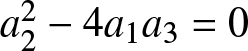 $a_2^2 - 4 a_1 a_3 = 0$. The characteristic polynomial can be rewritten in this setting as
 \begin{align}cp(\varepsilon \lambda_2, \varepsilon) & = \varepsilon^3 \left( a_1 \lambda_2^2 + a_2 \lambda_2 + a_3 + \mathcal{O}(\varepsilon) \right) \notag \\
& = \varepsilon^3 \left( a_1 (\lambda_2 - \lambda_2^*)^2 + \varepsilon R(\lambda_2) + \mathcal{O}(\varepsilon^{ \gt 1}) \right),\end{align}
where  $R(\lambda_2)$ is a quartic polynomial corresponding to the vertices
 $(0,4),(1,3),(2,2),(3,1),(4,0)$ in the Newton polytope. Writing
 \begin{equation*}
R(\lambda_2) := \lambda_2^4 + d_1 \lambda_2^3 + d_2 \lambda_2^2 + d_3 \lambda_2 + d_4
\end{equation*}
the coefficients  $d_i$ are found explicitly by using the symbolic software:
 \begin{equation*}
\begin{cases}
d_1 & = - b_{11} - b_{22} - b_{33} - b_{44}, \\
d_2 & =
- b_{12} b_{21}
+ b_{11} b_{22}
- b_{13} b_{31}
- b_{23} b_{32}
- b_{14} b_{41}
- b_{24} b_{42}
- b_{34} b_{43}
+ b_{33} b_{44} \\
& \quad \quad
+ b_{11} ( b_{33} + b_{44} )
+ b_{22} ( b_{33} + b_{44} )
- c_{43} \\
d_3 & = b_{13} b_{22} b_{31}
- b_{12} b_{23} b_{31}
- b_{13} b_{21} b_{32}
+ b_{11} b_{23} b_{32} \\[4pt]
& \quad \quad + b_{14} b_{22} b_{41}
- b_{12} b_{24} b_{41}
- b_{13} b_{34} b_{41}
- b_{14} b_{21} b_{42}
+ b_{11} b_{24} b_{42}
- b_{23} b_{34} b_{42} \\[4pt]
& \quad \quad + b_{11} b_{34} b_{43}
+ b_{22} b_{34} b_{43}
+ b_{11} b_{22} ( - b_{33} - b_{44} )
+ b_{12} b_{21} ( b_{33} + b_{44} ) \\[6pt]
& \quad \quad + b_{41} ( b_{14} b_{33} - c_{13} )
+ b_{43} ( - b_{14} b_{31} - b_{24} b_{32} + c_{11} + c_{22} )
+ b_{42} ( b_{24} b_{33} - c_{23} ) \\[4pt]
& \quad \quad + b_{13} ( b_{31} b_{44} - c_{41} )
+ b_{23} ( b_{32} b_{44} - c_{42} )
+ b_{11} ( - b_{33} b_{44} + c_{43} )
+ b_{22} ( - b_{33} b_{44} + c_{43} )\\
d_4 & = b_{13} b_{22} b_{34} b_{41}
- b_{12} b_{23} b_{34} b_{41}
- b_{13} b_{21} b_{34} b_{42}
+ b_{11} b_{23} b_{34} b_{42}
+ b_{12} b_{21} b_{34} b_{43}
- b_{11} b_{22} b_{34} b_{43} \\[4pt]
& + b_{22} b_{43} ( b_{14} b_{31} - c_{11} )
+ b_{23} b_{42} ( - b_{14} b_{31} + c_{11} )
+ b_{23} b_{41} ( b_{14} b_{32} - c_{12} )
+ b_{21} b_{43} ( - b_{14} b_{32} + c_{12} ) \\[4pt]
& + b_{21} b_{42} ( b_{14} b_{33} - c_{13} )
+ b_{22} b_{41} ( - b_{14} b_{33} + c_{13} )
+ b_{13} b_{42} ( b_{24} b_{31} - c_{21} )
+ b_{12} b_{43} ( - b_{24} b_{31} + c_{21} ) \\[4pt]
& + b_{11} b_{43} ( b_{24} b_{32} - c_{22} )
+ b_{13} b_{41} ( - b_{24} b_{32} + c_{22} )
+ b_{12} b_{41} ( b_{24} b_{33} - c_{23} )
+ b_{11} b_{42} ( - b_{24} b_{33} + c_{23} ) \\[4pt]
& + b_{12} b_{23} ( b_{31} b_{44} - c_{41} )
+ b_{13} b_{22} ( - b_{31} b_{44} + c_{41} )
+ b_{13} b_{21} ( b_{32} b_{44} - c_{42} )
+ b_{11} b_{23} ( - b_{32} b_{44} + c_{42} ) \\[4pt]
& + b_{11} b_{22} ( b_{33} b_{44} - c_{43} )
+ b_{12} b_{21} ( - b_{33} b_{44} + c_{43} )
\end{cases}
\end{equation*}
Now we set  $\lambda_2 = \lambda_2^* + \eta$ and expand (3.26):
 \begin{align*}
cp(\varepsilon \lambda_{2}, \varepsilon)= \varepsilon^{3}\left(a_{1} \eta^{2}+ \varepsilon \left(R(\lambda_{2}^{*})+ \eta R^{\prime}(\lambda_{2}^{*})+ \frac{1}{2}\eta^{2} R^{\prime\prime}(\lambda_{2}^{*})+ \frac{1}{6}\eta^{3} R^{\prime\prime\prime}(\lambda_2^{*})+ \eta^{4}\right)\right)+ \mathcal{O}(\varepsilon^{ \gt {3}}).
\end{align*}
Collecting terms yields the balance 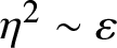 $\eta^2 \sim \varepsilon$ or
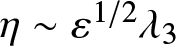 $\eta \sim \varepsilon^{1/2} \lambda_3$. Substituting this into the previous expression and collecting the leading order, we obtain
 \begin{equation*}
a_1 \lambda_3^2 + R(\lambda_2^*) = 0 \quad \quad \Rightarrow \quad \quad \lambda_3 = \pm \sqrt{\frac{R(\lambda_2^*)}{a_1}}.
\end{equation*}
Putting this all together now, we have that the double eigenvalue at the order of  $\mathcal{O}(\varepsilon)$ splits at the order of
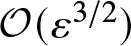 $\mathcal{O}(\varepsilon^{3/2})$ if
 $R(\lambda_2^*) \neq 0$ like
 \begin{equation}
\lambda \sim \pm \varepsilon^{1/2} \sqrt{b_{43}} \quad \textrm{and } \quad \lambda \sim \varepsilon \lambda_2^* \pm \varepsilon^{3/2} \sqrt{\frac{R(\lambda_2^*)}{a_1}}.
\end{equation}
The eigenvalue splitting (3.27) is obtained with direct Puiseux expansions, see (7.10) with (7.13) and (7.20) in Section 7.
4. Degeneration of figure-8 bands resulting in their vertical slope
The corresponding bifurcation is seen in panels (b)–(d) of Figure 1. Due to its shape, it can be called the hourglass bifurcation. Before the bifurcation [panel (b)], the spectral bands near  $\lambda = 0$ form a typical figure-
 $8$ pattern. At the bifurcation [panel (c)], the slopes of the figure-
 $8$ bands become vertical at
 $\lambda = 0$. After the bifurcation [panel (d)], the figure-
 $8$ bands break into two instability bubbles along the imaginary axis.
Section 4.1 develops the criterion for this bifurcation. Section 4.2 gives the derivation of the normal form, which explains how the bifurcation is unfolded. Section 4.3 describes numerical approximations of the coefficients of the normal form, from which we are able to reproduce the bifurcation pattern seen in panels (b)–(d) of Figure 1.
4.1. Criterion of the bifurcation
We study first the geometric and algebraic multiplicity of the eigenvalue  $\lambda = 0$ in the spectral problem (1.27) for
 $\mu = 0$. Recall that the two signs in (1.27) are defined for the two signs of
 $\mu$, hence,
 $\mu = 0$ stands for the limit
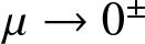 $\mu \to 0^{\pm}$, given by the spectral problem (2.12), see Remark 9.
For the geometric multiplicity of the zero eigenvalue, we add the following generic assumption.
Assumption 1.  ${\rm Ker}(\mathcal{L}) = {\rm span}(\eta')$ for this value of
 $c \in (1,c_*)$.
Since  $\mathcal{K} 1 = 0$ and
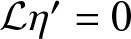 $\mathcal{L} \eta' = 0$ are satisfied for every
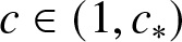 $c \in (1,c_*)$, Assumption 1 implies that the spectral problem (2.12) for
 $\lambda = 0$ admits a two-dimensional kernel spanned as
 \begin{equation}
\left( \begin{array}{c} \hat{v}_0 \\ \hat{w}_0 \end{array} \right) = a_1 \left( \begin{array}{c} \eta' \\ 0 \end{array} \right) + a_2 \left( \begin{array}{c} 0 \\ 1 \end{array} \right),
\end{equation}
where 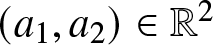 $(a_1,a_2) \in \mathbb{R}^2$. Due to the Hamiltonian symmetry in Lemma 1, the generalized kernel of the spectral problem (2.12) is at least four-dimensional with at least two generalized eigenfunctions. These generalized eigenfunctions were obtained in [Reference Dyachenko and Pelinovsky20] for the spectral problem (1.19) and can be extended to the spectral problem (2.12) by using the transformation (2.11) in Lemma 5 as follows:
 \begin{equation}
\left( \begin{array}{c} \hat{v}_g \\ \hat{w}_g \end{array} \right) = a_1
\left[ \left( \begin{array}{c} -\partial_c \eta \\ \mathcal{H} \eta \end{array} \right) \pm i \langle 1, \partial_c \eta \rangle
\left( \begin{array}{c} \eta' \\ -c \end{array} \right)
\right]
+ a_2 \left[ \left( \begin{array}{c} -1 \\ 0 \end{array} \right)
\pm i \left( \begin{array}{c} \eta' \\ -c \end{array} \right) \right],
\end{equation}
where the smoothness of the mapping 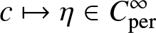 $c \mapsto \eta \in C^{\infty}_{\rm per}$ is due to Assumption 1, see Lemma 3. It can be checked by using (2.1) and (2.4) that
 $(\hat{v}_g,\hat{w}_g)$ satisfies the linear inhomogeneous system
 \begin{equation}
\left\{\begin{array}{ll}
\mathcal{K} \hat{w}_g &= \mathcal{M} \hat{v}_0, \\
\mathcal{L} \hat{v}_g &= \mathcal{M}^* \hat{w}_0 - 2 c \mathcal{H} \hat{v}_0.
\end{array}
\right.
\end{equation}
The system (4.3) follows by differentiating (2.12) in  $\lambda$ at
 $\lambda = 0$ and using
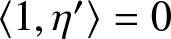 $\langle 1, \eta' \rangle = 0$. For the algebraic multiplicity of the zero eigenvalue, we add the following generic assumption.
Assumption 2. 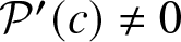 $\mathcal{P}'(c) \neq 0$ for this value of
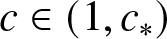 $c \in (1,c_*)$.
It is shown in [Reference Dyachenko and Pelinovsky20] that Assumptions 1 and 2 imply that the generalized kernel of the spectral problem (2.12) is exactly four-dimensional.
We now formulate and prove the criterion for the corresponding bifurcation.
Theorem 1 Let Assumptions 1 and 2 be true and set
 \begin{equation}
\Delta(c) := 4 \mathcal{P}'(c) \mathcal{N}(c) - 5 \mathcal{P}(c) \mathcal{N}'(c).
\end{equation}
There exist four spectral bands of the modulational stability problem (1.27) intersecting  $\lambda = 0$. Two of the spectral bands are subsets of
 $i \mathbb{R}$ and non-degenerate if
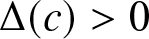 $\Delta(c) \gt 0$, tangential to
 $i \mathbb{R}$ and degenerate if
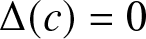 $\Delta(c) = 0$, and cross
 $\lambda = 0$ along the straight lines in all four complex quadrants of the complex
 $\lambda$-plane and non-degenerate if
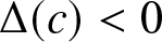 $\Delta(c) \lt 0$. The other two spectral bands are subsets of
 $i \mathbb{R}$ and non-degenerate, independently of
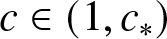 $c \in (1,c_*)$.
Proof. Substituting (4.1) into (1.27) yields the residual terms
 \begin{equation*}
\left\{\begin{array}{l}
i \mu \mathcal{H}_{\pm} \hat{w}_0 + \lambda \mathcal{M}_{\pm} \hat{v}_0, \\
i \mu \mathcal{L}_{\pm} \hat{v}_0 + \lambda (\mathcal{M}_{\pm}^* \hat{w}_0 - 2 c \mathcal{H}_{\pm} \hat{v}_0).
\end{array} \right.
\end{equation*}
Projecting the first equation to  ${\rm Ker}(\mathcal{K}) = {\rm span}(1)$ in the first equation and the second equation to
 ${\rm Ker}(\mathcal{L}) = {\rm span}(\eta')$ yields
 \begin{equation}
\left\{\begin{array}{l}
i\mu \langle 1, \mathcal{H}_{\pm} \hat{w}_0 \rangle + \lambda \langle 1, \mathcal{M}_{\pm} \hat{v}_0 \rangle, \\
i\mu \langle \eta', \mathcal{L}_{\pm} \hat{v}_0 \rangle
+ \lambda \langle \eta', (\mathcal{M}_{\pm}^* \hat{w}_0 - 2 c \mathcal{H}_{\pm} \hat{v}_0) \rangle,
\end{array} \right.
\end{equation}
Substituting 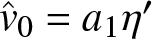 $\hat{v}_0 = a_1 \eta'$ and
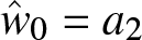 $\hat{w}_0 = a_2$ into (4.5) yields
 \begin{equation}
\left( \begin{matrix}
0 & \mp \mu \\
0 & 0
\end{matrix} \right) \left( \begin{matrix} a_1 \\ a_2 \end{matrix} \right),
\end{equation}
where we have used  $\langle \eta', \eta \rangle = \langle 1, \eta' \rangle = \langle \eta', \mathcal{K} \eta \rangle = 0$,
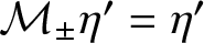 $\mathcal{M}_{\pm} \eta' = \eta'$,
 $\mathcal{L}_{\pm} \eta' = -\eta$, see (1.21), (1.23) and (2.3). The first-order terms in
 $\lambda$ have zero projections due to the existence of the generalized kernel given by (4.2). The first-order terms in
 $\mu$ have one nonzero projection and one zero projection.
In terms of analysis in Section 3.1, we can associate  $\mu$ as
 $\varepsilon$ and obtain (3.9) from (4.6). This suggests the eigenvalue splitting as in (3.13) with two eigenvalues of the order
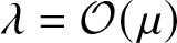 $\lambda = \mathcal{O}(\mu)$ related to the subspace
 $(a_1,a_2) = (1,0)$ and two eigenvalues of the order
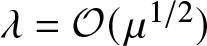 $\lambda = \mathcal{O}(\mu^{1/2})$ related to the subspace
 $(a_1,a_2) = (0,1)$. By using direct Puiseux expansions, it suffices to consider these two subspaces separately from each other, with two different expansions in powers of
 $\mu$. In what follows, we give the computational details which imply the assertion. Justification of the asymptotic expansions is based on the methods from [Reference Hinch25, Reference Hormander26, Reference Kirwan28] explained in Section 3.1.
 $\underline{\boldsymbol{\mathrm{Subspace}}\ (a_1,a_2) = (1,0)}$: We introduce the asymptotic expansions
 \begin{equation}
\mu = \epsilon \mu_1, \quad \lambda = \epsilon \lambda_1 + \mathcal{O}(\epsilon^2),
\end{equation}
and
 \begin{equation}
\left( \begin{array}{c} \hat{v} \\ \hat{w} \end{array} \right) = \left( \begin{array}{c} \eta' \\ 0 \end{array} \right) + \epsilon \left( \begin{array}{c} \hat{v}_1 \\ \hat{w}_1 \end{array} \right) + \epsilon^2 \left( \begin{array}{c} \hat{v}_2 \\ \hat{w}_2 \end{array} \right) + \mathcal{O}(\epsilon^3),
\end{equation}
where  $\epsilon \gt 0$ is a small parameter,
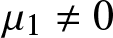 $\mu_1 \neq 0$ is fixed and the correction terms
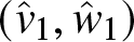 $(\hat{v}_1, \hat{w}_1)$ and
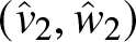 $(\hat{v}_2, \hat{w}_2)$ are to be computed recursively in function space
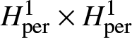 $H^1_{\rm per} \times H^1_{\rm per}$.
 $\underline{\boldsymbol{\mathrm{Order}} \ \mathcal{O}(\epsilon)}$: We get the linear inhomogeneous system
 \begin{equation}
\left\{\begin{array}{ll}
\mathcal{K} \hat{w}_1 &= \lambda_1 \mathcal{M} \eta', \\
\mathcal{L} \hat{v}_1 &= - 2 c \lambda_1 \mathcal{H} \eta' + i \mu_1 \mathcal{L}_{\pm} \eta' ,
\end{array}
\right.
\end{equation}
where the plus/minus signs correspond to  ${\rm sgn}(\mu_1) = \pm 1$. Since
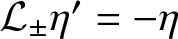 $\mathcal{L}_{\pm} \eta' = -\eta$ by (2.3) and
 \begin{equation}
\mathcal{L} \Upsilon = - \eta, \quad \Upsilon := \frac{c}{2} \partial_c \eta - \eta,
\end{equation}
by (2.2) and (2.4), we use (4.1) and (4.2) and obtain the solution in the form
 \begin{equation}
\left( \begin{array}{c} \hat{v}_1 \\ \hat{w}_1 \end{array} \right) = \lambda_1
\left[ \left( \begin{array}{c} -\partial_c \eta \\ \mathcal{H} \eta \end{array} \right) \pm i \langle 1, \partial_c \eta \rangle
\left( \begin{array}{c} \eta' \\ -c \end{array} \right)
\right]
+ i \mu_1 \left( \begin{array}{c} \Upsilon \\ 0 \end{array} \right)
+ a \left( \begin{array}{c} 0 \\ 1 \end{array} \right),
\end{equation}
where  $a \in \mathbb{R}$ is arbitrary at this order and the projection to
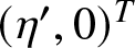 $(\eta',0)^T$ is not included since the eigenfunctions are defined up to arbitrary scalar multiplication in (4.8).
 $\underline{\boldsymbol{\mathrm{Order}} \ \mathcal{O}(\epsilon^2)}$: We get the linear inhomogeneous system
 \begin{equation}
\left\{\begin{array}{ll}
\mathcal{K} \hat{w}_2 &= \lambda_1 \left( \mathcal{M} \hat{v}_1 \pm i \langle 1, \hat{v}_1 \rangle \eta' \right) + i \mu_1 \left( \mathcal{H} \hat{w}_1 \pm i \langle 1, \hat{w}_1 \rangle \right), \\
\mathcal{L} \hat{v}_2 &= \lambda_1 \left( \mathcal{M}^* \hat{w}_1
- 2 c \mathcal{H} \hat{v}_1 \mp i \langle \eta', \hat{w}_1 \rangle \mp 2 c i \langle 1, \hat{v}_1 \rangle \right) + i \mu_1 \mathcal{L}_{\pm} \hat{v}_1.
\end{array}
\right.
\end{equation}
By Fredholm’s theorem, there exists a periodic solution of the linear inhomogeneous system (4.12) if and only if the two constraints are satisfied:
 \begin{equation}
\lambda_1 \langle 1, \mathcal{M} \hat{v}_1 \rangle \mp \mu_1 \langle 1, \hat{w}_1 \rangle = 0,
\end{equation}
 \begin{equation}
\lambda_1 \langle \eta', \mathcal{M}^* \hat{w}_1
- 2 c \mathcal{H} \hat{v}_1 \rangle + i \mu_1 \langle \eta', \mathcal{L}_{\pm} \hat{v}_1 \rangle = 0,
\end{equation}
where we have used  $\langle 1, \eta' \rangle = \langle 1, \mathcal{H} \hat{w}_1 \rangle = 0$. Taking derivative of the constraint (1.9) with respect to
 $c$ yields
 \begin{equation}
\langle (1+2K\eta), \partial_c \eta \rangle = 0.
\end{equation}
Since  $\mathcal{M}^* 1 = 1 + 2 \mathcal{K}\eta$, it follows from (4.11) and (4.13) with the help of (4.15) that
 \begin{equation}
i \mu_1 \lambda_1 \langle (1 + 2 \mathcal{K} \eta), \Upsilon \rangle
+ i c \mu_1 \lambda_1 \langle 1, \partial_c \eta \rangle \mp a \mu_1 = 0.
\end{equation}
By using (1.9), (2.1), (4.10) and self-adjointness of  $\mathcal{L}$, we get
 \begin{equation}
\langle (1 + 2 \mathcal{K} \eta), \Upsilon \rangle = - \langle \mathcal{L} 1, \Upsilon \rangle = -\langle 1, \mathcal{L} \Upsilon \rangle
= \langle 1, \eta \rangle = - \langle \mathcal{K} \eta, \eta \rangle.
\end{equation}
Dividing (4.16) by 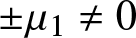 $\pm \mu_1 \neq 0$ and using (2.5), (4.15) and (4.17), we obtain the unique expression for
 $a$:
 \begin{align}
a &= \pm i \lambda_1 \left[ c \langle 1, \partial_c \eta \rangle - \langle \mathcal{K} \eta, \eta \rangle \right] \notag \\
&= \mp i \lambda_1 \left[ 2 c \langle K \eta, \partial_c \eta \rangle + \langle \mathcal{K} \eta, \eta \rangle \right] \notag \\
&= \mp i \lambda_1 \mathcal{P}'(c).
\end{align}
Similarly, it follows from (4.11) and (4.14) that  $(\mu_1,\lambda_1)$ must be related according to the characteristic equation:
 \begin{equation}
\lambda_1^2 \left[ \langle \mathcal{K} \eta, \eta \rangle + 2 c \langle \mathcal{K} \eta, \partial_c \eta \rangle \right] - i \mu_1 \lambda_1 \left[ \langle \eta, \partial_c \eta \rangle + 2 c \langle \mathcal{K}\eta, \Upsilon \rangle \right] - \mu_1^2 \langle \eta, \Upsilon \rangle = 0,
\end{equation}
where we have used 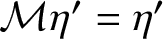 $\mathcal{M} \eta' = \eta'$ and
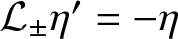 $\mathcal{L}_{\pm} \eta' = -\eta$ together with skew-adjointness of
 $\mathcal{H}$ and
 $\mathcal{L}_{\pm}$ in
 $L^2_{\rm per}$. Note that
 $a$ in (4.18) does not contribute to the equation (4.19). Substituting (4.10) into (4.19) and using (2.5) and (2.7) yields the quadratic characteristic equation
 \begin{equation}
\lambda_1^2 \mathcal{P}'(c) - i \mu_1 \lambda_1 \mathcal{N}'(c) + \mu_1^2 \left[ \mathcal{N}(c) - \frac{c}{4} \mathcal{N}'(c) \right] = 0,
\end{equation}
where we have used that
 \begin{equation*}
2c \langle \mathcal{K} \eta, \Upsilon \rangle = - \langle \mathcal{L} \partial_c \eta, \Upsilon \rangle = \langle \partial_c \eta, \eta \rangle,
\end{equation*}
due to (2.4) and (4.10) as well as self-adjointness of  $\mathcal{L}$ in
 $L^2_{\rm per}$. Note that the quadratic equation (4.20) is the same for both
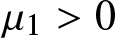 $\mu_1 \gt 0$ and
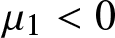 $\mu_1 \lt 0$. It admits two solutions
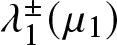 $\lambda_1^{\pm}(\mu_1)$ given by
 \begin{equation}
\lambda_1^{\pm}(\mu_1) = \frac{i \mu_1}{2 \mathcal{P}'(c)} \left[ \mathcal{N}'(c) \pm \sqrt{\Delta(c)}\right],
\end{equation}
where  $\Delta(c)$ is given by (4.4). If
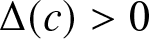 $\Delta(c) \gt 0$, then
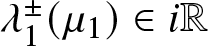 $\lambda_1^{\pm}(\mu_1) \in i \mathbb{R}$ and
 $\lambda_1^+(\mu_1) \neq \lambda_2^-(\mu_1)$ for
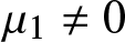 $\mu_1 \neq 0$. If
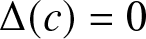 $\Delta(c) = 0$, then
 $\lambda_1^{\pm}(\mu_1) \in i \mathbb{R}$ and
 $\lambda_1^+(\mu_1) = \lambda_2^-(\mu_1)$ for
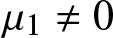 $\mu_1 \neq 0$. If
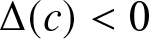 $\Delta(c) \lt 0$, then
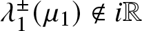 $\lambda_1^{\pm}(\mu_1) \notin i \mathbb{R}$.
Persistence of the two spectral bands crossing  $\lambda = 0$ for
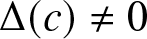 $\Delta(c) \neq 0$ follows from the Hamiltonian symmetry of Lemma 2. For fixed
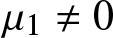 $\mu_1 \neq 0$, the two eigenvalues
 $\lambda_1^{\pm}$ are distinct and hence they remain either on
 $i \mathbb{R}$ if
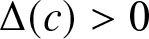 $\Delta(c) \gt 0$ or in each quadrant of the complex
 $\lambda$-plane if
 $\Delta(c) \lt 0$, in the asymptotic expansions (4.7) and (4.8).
 $\underline{\boldsymbol{\mathrm{Subspace}} \ (a_1,a_2) = (0,1)}$: We introduce the asymptotic expansions
 \begin{equation}
\mu = \epsilon^2 \mu_2, \quad \lambda = \epsilon \lambda_1 + \mathcal{O}(\epsilon^2),
\end{equation}
and
 \begin{equation}
\left( \begin{array}{c} \hat{v} \\ \hat{w} \end{array} \right) = \left( \begin{array}{c} 0 \\ 1 \end{array} \right) + \epsilon \left( \begin{array}{c} \hat{v}_1 \\ \hat{w}_1 \end{array} \right) + \epsilon^2 \left( \begin{array}{c} \hat{v}_2 \\ \hat{w}_2 \end{array} \right) + \mathcal{O}(\epsilon^3).
\end{equation}
where  $\epsilon \gt 0$ is a small parameter,
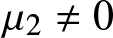 $\mu_2 \neq 0$ is fixed and the correction terms
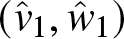 $(\hat{v}_1, \hat{w}_1)$ and
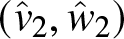 $(\hat{v}_2, \hat{w}_2)$ are to be computed recursively in function space
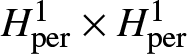 $H^1_{\rm per} \times H^1_{\rm per}$.
 $\underline{\boldsymbol{\mathrm{Order}} \ \mathcal{O}(\epsilon)}$: We use (4.1) and (4.2) and obtain the solution in the form
 \begin{equation}
\left( \begin{array}{c} \hat{v}_1 \\ \hat{w}_1 \end{array} \right) = \lambda_1
\left[ \left( \begin{array}{c} -1 \\ 0 \end{array} \right) \pm i
\left( \begin{array}{c} \eta' \\ -c \end{array} \right)
\right]
+ a \left( \begin{array}{c} \eta' \\ 0 \end{array} \right),
\end{equation}
where  $a \in \mathbb{R}$ is arbitrary at this order and the projection to
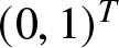 $(0,1)^T$ is not included since the eigenfunctions are defined up to arbitrary scalar multiplication in (4.23).
 $\underline{\boldsymbol{\mathrm{Order}} \ \mathcal{O}(\epsilon^2)}$: We get the linear inhomogeneous system
 \begin{equation}
\left\{\begin{array}{ll}
\mathcal{K} \hat{w}_2 &= i \mu_2 \mathcal{H}_{\pm} 1 + \lambda_1 \mathcal{M}_{\pm} \hat{v}_1, \\
\mathcal{L} \hat{v}_2 &= \lambda_1 \left( \mathcal{M}^*_{\pm} \hat{w}_1
- 2 c \mathcal{H}_{\pm} \hat{v}_1 \right).
\end{array}
\right.
\end{equation}
Fredholm’s orthogonality condition to the first equation of system (4.25) gives
 \begin{equation}
\mp \mu_2 - \lambda_1^2 \langle 1, \mathcal{M} 1 \rangle = 0 \quad \Rightarrow \quad \lambda_1^2 = -|\mu_2|,
\end{equation}
where we have used  $\mathcal{M} 1 = 1 + \mathcal{K} \eta$ and
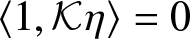 $\langle 1, \mathcal{K} \eta \rangle = 0$. Fredholm’s orthogonality condition to the second equation of system (4.25) is trivially satisfied because
 \begin{equation*}
\langle \eta', \mathcal{M}^*_{\pm} \hat{w}_1 - 2 c \mathcal{H}_{\pm} \hat{v}_1 \rangle =
\langle \eta', \hat{w}_1 \rangle - 2 c \langle \mathcal{K} \eta, \hat{v}_1 \rangle = 0.
\end{equation*}
The two solutions  $\lambda_1^{\pm}(\mu_2) = \pm i \sqrt{|\mu_2|} \in i \mathbb{R}$ satisfy
 $\lambda_1^+(\mu_2) \neq \lambda_1^-(\mu_2)$ for
 $\mu_2 \neq 0$. Under the orthogonality condition
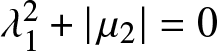 $\lambda_1^2 + |\mu_2| = 0$, the system (4.25) can be solved explicitly:
 \begin{equation}
\left( \begin{array}{c} \hat{v}_2 \\ \hat{w}_2 \end{array} \right) = \lambda_1^2
\left( \begin{array}{c} \pm i (\partial_c \eta - c) \\ -\eta \end{array} \right)
+ a \lambda_1 \left[ \left( \begin{array}{c} -\partial_c \eta \\ \mathcal{H} \eta \end{array} \right) \pm i \langle 1, \partial_c \eta \rangle \left( \begin{array}{c} \eta' \\ -c \end{array} \right) \right],
\end{equation}
where we have used  $\mathcal{L}(\partial_c \eta - c) = c$, which follows from (2.1) and (2.4). The parameter
 $a \in \mathbb{R}$ is not defined in (4.24) and (4.27) up to the order
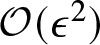 $\mathcal{O}(\epsilon^2)$. Since
 $\lambda_1^+(\mu_2) \neq \lambda_1^-(\mu_2)$ for
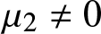 $\mu_2 \neq 0$, the two spectral bands persist on
 $i \mathbb{R}$ in the asymptotic expansions (4.22) and (4.23) due to the Hamiltonian symmetry of Lemma 2.
Remark 10. If  $\Delta(c) \lt 0$, the spectral bands in Theorem 1 crossing
 $\lambda = 0$ can be parts of either figure-
 $8$ or figure-
 $\infty$ or a more complicated pattern. If
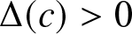 $\Delta(c) \gt 0$, the spectral bands on
 $i \mathbb{R}$ near
 $\lambda = 0$ may become complex away from
 $\lambda = 0$ due to additional bifurcations of the instability bubbles on
 $i \mathbb{R}$. If
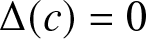 $\Delta(c) = 0$, we have the bifurcation for which the degenerate figure-8 bands have the vertical slope at
 $\lambda = 0$. Computation of the normal form of this bifurcation is required to unfold the degeneracy beyond the leading order and to obtain further information on whether the spectral bands are subsets of
 $i \mathbb{R}$ near
 $\lambda = 0$ or cross
 $\lambda = 0$ from the four complex quadrants of the complex
 $\lambda$-plane, see Theorem 2 below.
4.2. Normal form for the bifurcation
The normal form takes into account higher-order terms in  $\mu$ which break the degeneracy of the double eigenvalue
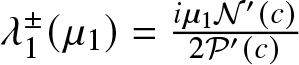 $\lambda_1^{\pm}(\mu_1) = \frac{i \mu_1 \mathcal{N}'(c)}{2 \mathcal{P}'(c)}$ in the case of
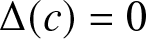 $\Delta(c) = 0$, see Remark 10. This is done by continuing Puiseux expansions to higher orders in
 $\epsilon$, as in Section 3.4. The following theorem gives the normal form with a numerical coefficient
 $\mathcal{D}$, which is assumed to be non-zero for non-degeneracy.
Theorem 2 Under the assumptions of Theorem 1, let 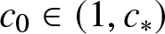 $c_0 \in (1,c_*)$ be the root of
 $\Delta(c)$ given by (4.4). Let
 $\mathcal{D}$ be given by (4.40) and assume that
 $\mathcal{D} \neq 0$. The two spectral bands intersecting
 $\lambda = 0$ with the vertical slope at
 $c = c_0$ are non-degenerate and obtained from roots of the characteristic equation
 \begin{equation}
\mathcal{P}'(c_0) \left( \lambda - \frac{i \mu \mathcal{N}'(c_0)}{2 \mathcal{P}'(c_0)} \right)^2 + \mathcal{D} |\mu|^3 = \mathcal{O}(\mu^4).
\end{equation}
If  ${\rm sgn}\mathcal{D} = {\rm sgn} \mathcal{P}'(c_0)$, the two spectral bands are subsets of
 $i \mathbb{R}$. If
 ${\rm sgn}\mathcal{D} = -{\rm sgn} \mathcal{P}'(c_0)$, the two spectral bands cross
 $\lambda = 0$ along the straight lines in all four complex quadrants of the complex
 $\lambda$-plane.
Proof. By using Puiseux expansions for the double eigenvalue  $\lambda_1^+(\mu_1) = \lambda_2^-(\mu_1)$ in (4.21) with
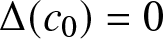 $\Delta(c_0) = 0$, we modify the expansions (4.7) and (4.8) as follows:
 \begin{equation}
\mu = \epsilon \mu_1, \quad \lambda = \epsilon \lambda_1 + \epsilon^{3/2} \lambda_{3/2} + \mathcal{O}(\epsilon^2),
\end{equation}
and
 \begin{align}\left( \begin{array}{c} \hat{v} \\ \hat{w} \end{array} \right) &= \left( \begin{array}{c} \eta' \\ 0 \end{array} \right) + \epsilon \left( \begin{array}{c} \hat{v}_1 \\ \hat{w}_1 \end{array} \right) + \epsilon^{3/2} \left( \begin{array}{c} \hat{v}_{3/2} \\ \hat{w}_{3/2} \end{array} \right) + \epsilon^2 \left( \begin{array}{c} \hat{v}_2 \\ \hat{w}_2 \end{array} \right) \notag \\
& \quad + \epsilon^{5/2} \left( \begin{array}{c} \hat{v}_{5/2} \\ \hat{w}_{5/2} \end{array} \right) + \epsilon^2 \left( \begin{array}{c} \hat{v}_3 \\ \hat{w}_3 \end{array} \right) + \mathcal{O}(\epsilon^{7/2}).\end{align}
We get the same solutions for the first two correction terms as in (4.11):
 \begin{equation}
\left( \begin{array}{c} \hat{v}_1 \\ \hat{w}_1 \end{array} \right) = \lambda_1
\left( \begin{array}{c} \tilde{v}_1 \\ \tilde{w}_1 \end{array} \right) + i \mu_1 \left( \begin{array}{c} \Upsilon \\ 0 \end{array} \right)
+ a_1 \left( \begin{array}{c} 0 \\ 1 \end{array} \right),
\end{equation}
and
 \begin{equation}
\left( \begin{array}{c} \hat{v}_{3/2} \\ \hat{w}_{3/2} \end{array} \right) = \lambda_{3/2}
\left( \begin{array}{c} \tilde{v}_1 \\ \tilde{w}_1 \end{array} \right) + a_{3/2} \left( \begin{array}{c} 0 \\ 1 \end{array} \right),
\end{equation}
where
 \begin{align*}
\left\{\begin{array}{l} \tilde{v}_1 = -\partial_c \eta \pm i \langle 1, \partial_c \eta \rangle \eta', \\
\tilde{w}_1 = \mathcal{H} \eta \mp i c \langle 1, \partial_c \eta \rangle.
\end{array} \right.
\end{align*}
We recall from (4.18) and (4.21) with 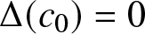 $\Delta(c_0) = 0$ that
 $a_1 = \mp i \lambda_1 \mathcal{P}'(c_0)$ and
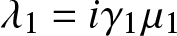 $\lambda_1 = i \gamma_1 \mu_1$ with
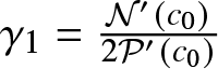 $\gamma_1 = \frac{\mathcal{N}'(c_0)}{2 \mathcal{P}'(c_0)}$. The parameter
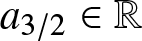 $a_{3/2} \in \mathbb{R}$ is arbitrary at this order. The linear inhomogeneous system (4.12) is solvable under the two conditions on
 $a$ and
 $\lambda_1$ so that we can define the solution in the implicit form:
 \begin{equation}
\left( \begin{array}{c} \hat{v}_2 \\ \hat{w}_2 \end{array} \right) = \mu_1^2
\left( \begin{array}{c} \tilde{v}_2 \\ \tilde{w}_2 \end{array} \right)
+ a_2 \left( \begin{array}{c} 0 \\ 1 \end{array} \right),
\end{equation}
where the coefficient 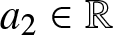 $a_2\in \mathbb{R}$ is arbitrary at this order and
 $(\tilde{v}_2,\tilde{w}_2) \in H^1_{\rm per} \times H^1_{\rm per}$ is uniquely determined from solutions of the linear inhomogeneous system
 \begin{equation}
\left\{\begin{array}{ll}
\mathcal{K} \tilde{w}_2 &= -\gamma_1^2 \mathcal{M}_{\pm} \tilde{v}_1 - \gamma_1 \mathcal{M}_{\pm} \Upsilon - \gamma_1 \mathcal{H}_{\pm}
\left( \tilde{w}_1 \mp i \mathcal{P}'(c_0) \right), \\
\mathcal{L} \tilde{v}_2 &= -\gamma_1^2 \left( \mathcal{M}_{\pm}^* \tilde{w}_1 \mp i \mathcal{P}'(c_0) \mathcal{M}^* 1
- 2 c \mathcal{H}_{\pm} \tilde{v}_1 \right) + 2 c \gamma_1 \mathcal{H}_{\pm} \Upsilon - \gamma_1 \mathcal{L}_{\pm} \tilde{v}_1 - \mathcal{L}_{\pm} \Upsilon,
\end{array}
\right.
\end{equation}
under the orthogonality conditions  $\langle 1, \hat{w}_2 \rangle = \langle \eta', \hat{v}_2 \rangle = 0$.
 $\underline{\boldsymbol{\mathrm{Order}} \ \mathcal{O}(\epsilon^{5/2})}$: We get the linear inhomogeneous system
 \begin{equation}
\left\{\begin{array}{ll}
\mathcal{K} \hat{w}_{5/2} &= 2 \lambda_1 \lambda_{3/2} \mathcal{M}_{\pm} \tilde{v}_1 +
i \mu_1 \left( \lambda_{3/2} \mathcal{H}_{\pm} \tilde{w}_1 + a_{3/2} \mathcal{H}_{\pm} 1 \right), \\
\mathcal{L} \hat{v}_{5/2} &= 2 \lambda_1 \lambda_{3/2} \left( \mathcal{M}_{\pm}^* \tilde{w}_{1}
- 2 c \mathcal{H}_{\pm} \tilde{v}_{1} \right) + (\lambda_1 a_{3/2} + \lambda_{3/2} a_1) \mathcal{M}_{\pm}^* 1 \\
& \qquad
- 2 c i \mu_1 \lambda_{3/2} \mathcal{H}_{\pm} \Upsilon + i \mu_1 \lambda_{3/2} \mathcal{L}_{\pm} \tilde{v}_{1}.
\end{array}
\right.
\end{equation}
The Fredholm condition for the first equation of the system (4.35) yields
 \begin{equation*}
a_{3/2} = \pm i \lambda_{3/2} c \langle 1, \partial_c \eta \rangle,
\end{equation*}
which simply implies that the correction term in (4.32) can be rewritten in the form
 \begin{equation}
\left( \begin{array}{c} \hat{v}_{3/2} \\ \hat{w}_{3/2} \end{array} \right) = \lambda_{3/2}
\left( \begin{array}{c} \tilde{v}_1 \\ \mathcal{H} \eta \end{array} \right).
\end{equation}
The Fredholm condition for the second equation of the system (4.35) yields
 \begin{align*}
0 &= \langle \eta', 2 \lambda_1 \lambda_{3/2} \left( \mathcal{M}_{\pm}^* \tilde{w}_{1}
- 2 c \mathcal{H}_{\pm} \tilde{v}_{1} \right)
- 2 c i \mu_1 \lambda_{3/2} \mathcal{H}_{\pm} \Upsilon + i \mu_1 \lambda_{3/2} \mathcal{L}_{\pm} \tilde{v}_{1} \rangle \\
&= 2 \lambda_1 \lambda_{3/2} \left[ \langle \eta', \mathcal{H} \eta \rangle + 2 c \langle \eta', \mathcal{H} \partial_c \eta \rangle \right]
- i \mu_1 \lambda_{3/2} \left[ \langle \eta, \partial_c \eta \rangle + 2 c \langle \mathcal{K} \eta, \Upsilon \rangle \right]\\
&= \lambda_{3/2} \left[ 2 \lambda_1 \mathcal{P}'(c_0) - i \mu_1 \mathcal{N}'(c_0) \right].
\end{align*}
This condition is equivalent to the derivative of the quadratic characteristic equation (4.20) in  $\lambda_1$ and it is trivially satisfied since
 $\lambda_1 = i \gamma_1 \mu_1$ is a double root of the characteristic equation (4.20) with
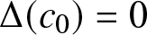 $\Delta(c_0) = 0$. Hence, we write the solution in the implicit form:
 \begin{equation}
\left( \begin{array}{c} \hat{v}_{5/2} \\ \hat{w}_{5/2} \end{array} \right) = \mu_1 \lambda_{3/2}
\left( \begin{array}{c} \tilde{v}_{5/2} \\ \tilde{w}_{5/2} \end{array} \right) + a_{5/2} \left( \begin{array}{c} 0 \\ 1 \end{array} \right),
\end{equation}
where the coefficient 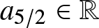 $a_{5/2} \in \mathbb{R}$ is arbitrary at this order and
 $(\tilde{v}_{5/2},\tilde{w}_{5/2}) \in H^1_{\rm per} \times H^1_{\rm per}$ is uniquely determined from solution of the linear inhomogeneous system
 \begin{equation*}
\left\{\begin{array}{ll}
\mathcal{K} \tilde{w}_{5/2} &= 2 i \gamma_1 \mathcal{M}_{\pm} \tilde{v}_1 +
+ i \mathcal{H}_{\pm} \mathcal{H} \eta, \\
\mathcal{L} \tilde{v}_{5/2} &= 2 i \gamma_1 \left( \mathcal{M}_{\pm}^* \tilde{w}_{1}
- 2 c \mathcal{H}_{\pm} \tilde{v}_{1} \right) \pm \gamma_1 (\mathcal{P}'(c_0) - c \langle 1, \partial_c \eta \rangle) \mathcal{M}_{\pm}^* 1 \\
& \qquad
- 2 c i \mathcal{H}_{\pm} \Upsilon + i \mathcal{L}_{\pm} \tilde{v}_{1},
\end{array}
\right.
\end{equation*}
under the orthogonality conditions  $\langle 1, \hat{w}_{5/2} \rangle = \langle \eta', \hat{v}_{5/2} \rangle = 0$.
 $\underline{\boldsymbol{\mathrm{Order}} \ \mathcal{O}(\epsilon^3)}$: We get the linear inhomogeneous system
 \begin{equation}
\left\{\begin{array}{ll}
\mathcal{K} \hat{w}_3 &= \lambda_1 \mathcal{M}_{\pm} \hat{v}_2 + \lambda_{3/2} \mathcal{M}_{\pm} \hat{v}_{3/2} +
i \mu_1 \mathcal{H}_{\pm} \hat{w}_{2}, \\
\mathcal{L} \hat{v}_3 &= \lambda_1 \left( \mathcal{M}_{\pm}^* \hat{w}_{2}
- 2 c \mathcal{H}_{\pm} \hat{v}_{2} \right) + \lambda_{3/2} \left( \mathcal{M}_{\pm}^* \hat{w}_{3/2}
- 2 c \mathcal{H}_{\pm} \hat{v}_{3/2} \right) + i \mu_1 \mathcal{L}_{\pm} \hat{v}_{2}.
\end{array}
\right.
\end{equation}
The Fredholm condition for the first equation of the system (4.38) yields a unique value for the coefficient  $a_2$. Since it does not affect the computations of the second equation, we do not write it explicitly. The Fredholm condition for the second equation of the system (4.38) yields the characteristic equation for
 $\lambda_{3/2}$:
 \begin{align}
0 &= \langle \eta', \lambda_1 \left( \mathcal{M}_{\pm}^* \hat{w}_{2}
- 2 c \mathcal{H}_{\pm} \hat{v}_{2} \right) + \lambda_{3/2} \left( \mathcal{M}_{\pm}^* \hat{w}_{3/2}
- 2 c \mathcal{H}_{\pm} \hat{v}_{3/2} \right) + i \mu_1 \mathcal{L}_{\pm} \hat{v}_{2} \rangle \notag \\
&= \lambda_1 \mu_1^2 \left[ \langle \eta', \tilde{w}_2 \rangle - 2 c \langle \eta', \mathcal{H} \tilde{v}_2 \rangle \right]
+ \lambda_{3/2}^2 \left[ \langle \eta', \mathcal{H} \eta \rangle + 2 c \langle \eta', \mathcal{H} \partial_c \eta \rangle \right]
+ i \mu_1^3 \langle \eta, \tilde{v}_2 \rangle \notag \\
&= \lambda_{3/2}^2 \mathcal{P}'(c_0) + i \mu_1^3 \left[ \gamma_1 \langle \eta', \tilde{w}_2 \rangle - 2 c \gamma_1 \langle \eta', \mathcal{H} \tilde{v}_2
\rangle + \langle \eta, \tilde{v}_2 \rangle \right].
\end{align}
In order to get (4.28) with an explicit expression for the numerical coefficient  $\mathcal{D}$, we need to extract the odd part of
 $\tilde{w}_2$ and the even part of
 $\tilde{v}_2$ from solutions of the linear inhomogeneous equation (4.34). We compute
 \begin{align*}
\mathcal{M}_{\pm} \tilde{v}_1 = -\mathcal{M} \partial_c \eta, \quad
\mathcal{M}_{\pm} \Upsilon &= \mathcal{M} \Upsilon \pm i \langle 1, \Upsilon \rangle \eta',
\end{align*}
and
 \begin{align*}
\mathcal{H}_{\pm} \left( \tilde{w}_1 \mp i \mathcal{P}'(c_0) \right) &= \mathcal{H} \mathcal{H} \eta + \mathcal{P}'(c_0) + c \langle 1, \partial_c \eta \rangle.
\end{align*}
Since  $\mathcal{K}$,
 $\mathcal{M}$ and
 $\mathcal{H} \mathcal{H}$ are parity preserving, the odd component of
 $\tilde{w}_2$ denoted as
 $\tilde{w}^{\rm odd}$ is given by a solution of the linear inhomogeneous equation
 \begin{equation*}
\mathcal{K} \tilde{w}_2^{\rm odd} = \mp i \gamma_1 \langle 1, \Upsilon \rangle \eta',
\end{equation*}
which yields  $\tilde{w}_2^{\rm odd} = \mp i \gamma_1 \langle 1, \Upsilon \rangle \mathcal{H} \eta$. Similarly, we compute
 \begin{align*}
\mathcal{M}^*_{\pm} \tilde{w}_1 &= \mathcal{M}^* \mathcal{H} \eta \mp i c \langle 1, \partial_c \eta \rangle (1 + 2 \mathcal{K} \eta)
\pm i \langle \mathcal{K} \eta, \eta \rangle, \\
\mathcal{H}^*_{\pm} \tilde{v}_1 &= - \mathcal{H} \partial_c \eta \mp i \langle 1, \partial_c \eta \rangle (1 + \mathcal{K} \eta), \\
\mathcal{L}_{\pm} \tilde{v}_1 &= -c^2 \mathcal{H} \partial_c \eta \mp i c^2 \langle 1, \partial_c \eta \rangle (1 + \mathcal{K} \eta)
+ \eta \mathcal{H} \partial_c \eta \pm i \langle 1, \partial_c \eta \rangle \eta (1 + \mathcal{K} \eta) \\
& \qquad
+ \mathcal{H} (\eta \partial_c \eta) \mp i \langle 1, \partial_c \eta \rangle \mathcal{H} (\eta \eta') \pm i \langle \eta, \partial_c \eta \rangle,
\end{align*}
and
 \begin{align*}
\mathcal{L}_{\pm} \Upsilon &= c^2 \mathcal{H} \Upsilon \pm i c^2 \langle 1, \Upsilon \rangle - \eta \mathcal{H} \Upsilon \mp i \langle 1, \Upsilon \rangle \eta
- \mathcal{H} (\eta \Upsilon) \mp i \langle \eta, \Upsilon \rangle.
\end{align*}
We note again that  $\mathcal{K}$,
 $\mathcal{L}$ and
 $\mathcal{M}^*$ are parity preserving, and that the even component in the right-hand sides alternate signs. Hence, the even component of
 $\tilde{v}_2$ denoted as
 $\tilde{v}^{\rm even}$ is given by
 $\tilde{v}_2^{\rm even} = \pm i \check{v}_2^{\rm even}$, where
 $\check{v}_2^{\rm even}$ is real, even, and uniquely defined from a solution of the linear inhomogeneous equation
 \begin{align*}
\mathcal{L} \check{v}_2^{\rm even} &= \gamma_1^2 c \langle 1, \partial_c \eta \rangle (1 + 2 \mathcal{K} \eta)
- \gamma_1^2 \langle \mathcal{K} \eta, \eta \rangle + \gamma_1^2 \mathcal{P}'(c_0) (1 + 2 \mathcal{K} \eta)
- 2 c \gamma_1^2 \langle 1, \partial_c \eta \rangle (1 + \mathcal{K} \eta) \\
& \quad + 2 c \gamma_1 \langle 1, \Upsilon \rangle + \gamma_1 c^2 \langle 1, \partial_c \eta \rangle (1 + \mathcal{K} \eta)
- \gamma_1 \langle 1, \partial_c \eta \rangle \eta (1 + \mathcal{K} \eta)
+ \gamma_1 \langle 1, \partial_c \eta \rangle \mathcal{H} (\eta \eta') \\
& \quad - \gamma_1 \langle \eta, \partial_c \eta \rangle - c^2 \langle 1, \Upsilon \rangle - \langle 1, \Upsilon \rangle \eta + \langle \eta, \Upsilon \rangle.
\end{align*}
By using (4.39), we obtain
 \begin{equation*}
\lambda_{3/2}^2 \mathcal{P}'(c_0) \pm \mu_1^3 \mathcal{D} = 0,
\end{equation*}
with
 \begin{equation}
\mathcal{D} = \gamma_1^2 \langle \mathcal{K} \eta, \eta\rangle \langle 1, \Upsilon \rangle + 2 c \gamma_1 \langle \mathcal{K} \eta, \check{v}_2^{\rm even}
\rangle - \langle \eta, \tilde{v}_2^{\rm even}\rangle.
\end{equation}
In view of the expansion (4.29), we obtain the normal form (4.28). The asymptotic expansions (4.30) is given by (4.31), (4.32), (4.33), (4.36) and (4.37). If  ${\rm sgn}\mathcal{D} = {\rm sgn} \mathcal{P}'(c_0)$, the two spectral bands are non-degenerate and persist on subsets of
 $i \mathbb{R}$ due to the Hamiltonian symmetry of Lemma 2. If
 ${\rm sgn}\mathcal{D} = -{\rm sgn} \mathcal{P}'(c_0)$, the two spectral bands are non-degenerate and persist in all four complex quadrants of the complex
 $\lambda$-plane.
Remark 11. Combining (4.21) and (4.28) yields
 \begin{equation}
\mathcal{P}'(c) \left( \lambda - \frac{i \mu \mathcal{N}'(c)}{2 \mathcal{P}'(c)} \right)^2 + \frac{\mu^2 \Delta(c)}{4 \mathcal{P}'(c)}
+ \mathcal{D} |\mu|^3 = \mathcal{O}(\mu^4),
\end{equation}
where  $\mathcal{D}$ is only defined at
 $c = c_0$ and
 $c_0$ is a root of
 $\Delta(c)$ in Theorem 2. Assume that
 $c_0$ is a simple root of
 $\Delta(c)$ with
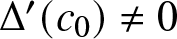 $\Delta'(c_0) \neq 0$, see Figure 2. Expanding (4.41) in
 $c$ near
 $c_0$ by using the smoothness of the mapping
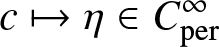 $c \mapsto \eta \in C^{\infty}_{\rm per}$, we obtain the extended normal form:
 \begin{equation}
\mathcal{P}'(c_0) \left( \lambda - \frac{i \mu \mathcal{N}'(c)}{2 \mathcal{P}'(c)} \right)^2 + \frac{\mu^2 \Delta'(c_0) (c - c_0)}{4 \mathcal{P}'(c_0)} + \mathcal{D} |\mu|^3 = \mathcal{O}(\mu^4),
\end{equation}
where the leading-order balance implies that  $c - c_0 = \mathcal{O}(\mu)$.
4.3. Numerical results
The criterion for the bifurcation is a simple zero of  $\Delta(c)$ defined by (4.4). The graph of
 $\Delta(c)$ versus wave steepness
 $s$ is shown in Figure 2 by a green solid line. Newton’s method is further used to improve the accuracy of finding
 $c_0$ at which
 $\Delta(c)$ vanishes. The corresponding values of
 $s_0$ and
 $c_0$ for the first two zeros of
 $\Delta$ are recorded in Table 2, where we also show the values of
 $\mathcal{P}'(c_0)$,
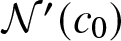 $\mathcal{N}'(c_0)$,
 $\mathcal{D}$ and
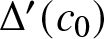 $\Delta'(c_0)$ in the normal form (4.28). We note that
 ${\rm sgn} \mathcal{D} = -{\rm sgn}\mathcal{P}'(c_0)$ so that the two spectral bands with the vertical slope cross
 $\lambda = 0$ along the straight lines in all four quadrants of the complex
 $\lambda$-plane, see Theorem 2. The sign alternation of
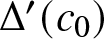 $\Delta'(c_0)$ is due to the fact that the mapping
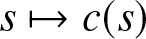 $s \mapsto c(s)$ is increasing at the first hourglass bifurcation and decreasing at the second hourglass bifurcation.
Parameters of the first two hourglass bifurcations

Table 2 Long description
Six columns list s0, c0, P prime at c0, N prime at c0, D, and Delta prime at c0 for two entries. Row 1 has s0 0.10921308 and c0 1.06052068, with P prime 4.618 and N prime 3.2142. In row 1, D is negative 1.804 times 10 to the minus 2, and Delta prime is 42.51. Row 2 has s0 0.14010224 and c0 1.09256435, with P prime 4.653 and N prime 2.8766. In row 2, D is negative 2.562 times 10 to the minus 2, and Delta prime is negative 8.818 times 10 to the 3. From row 1 to row 2, s0, c0, and P prime increase, N prime decreases, D becomes more negative, and Delta prime changes sign and increases greatly in magnitude.
Figures 9 and 10 show the instability bands of the spectral problem (1.27) near the origin in the spectral  $\lambda$-plane obtained numerically. The solid blue, green and red curves in each figure correspond to three consequent values of steepness before, at, and after the critical steepness, for which
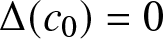 $\Delta(c_0) = 0$. The dashed lines display the spectral bands obtained from the normal form (4.42), where the value of
 $\mathcal{D}$ was computed by fitting the real part of
 $\lambda$ to the numerical data at
 $\Delta(c_0) = 0$ from equation (4.28), instead of using the projection formulas in (4.40). A good agreement between the spectral bands given by the normal form (4.42) and the numerical approximations of the stability spectra is evident for the first two cycles of bifurcations.
The first instance of the hourglass bifurcation, which corresponds to panels (b)–(d) of Figure 1 zoomed near the origin in the  $\lambda$-plane. The figure-
 $8$ for
 $c^- = 1.05970 \lt c_0$ (left panel) gets vertical slopes at the origin when
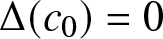 $\Delta(c_0) = 0$ for
 $c_0 \approx 1.06052068$ (middle panel), and splits into a pair of isolas along
 $i \mathbb{R}$ for
 $c^+ = 1.06135 \gt c_0$ (right panel). The dashed lines show the approximations obtained from the normal form (4.42).

The same as Figure 9 but for the second instance of the hourglass bifurcation, which happens when 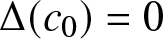 $\Delta(c_0) = 0$ for
 $c_0 \approx 1.09256435$.

5. New circular bands around the origin
The corresponding bifurcation is seen in panels (e)–(g) of Figure 1. Due to its shape, it can be called the ellipse bifurcation. Before the bifurcation [panel (e)], there are no circular bands around the origin. At the bifurcation [panel (f)], a new circular band appears from the origin and surrounds it. After the bifurcation [panel (g)], the new circular band grows in size.
Section 5.1 develops the criterion for this bifurcation. Section 5.2 gives the derivation of the normal form, which explains how the bifurcation is unfolded. Section 5.3 describes numerical approximations of the coefficients of the normal form, from which we are able to reproduce the bifurcation pattern seen in panels (e)–(g) of Figure 1.
5.1. Criterion of the bifurcation
This bifurcation arises due to the zero eigenvalue of the linearized operator  $\mathcal{L}$ extended to the space of double-periodic (antiperiodic) perturbations and denoted as
 $\mathcal{L}_{\rm aper}$. This linearized operator generally has no zero eigenvalues. However, zero eigenvalues appear in the continuation of the travelling wave with respect to the steepness parameter
 $s$, as was shown in [Reference Buffoni, Dancer and Toland11]. Hence, we add the following non-generic assumption for the bifurcation.
Assumption 3. For the given value of 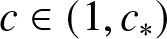 $c \in (1,c_*)$, there exists an eigenfunction
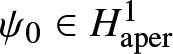 $\psi_0 \in H^1_{\rm aper}$ (defined up to scalar multiplication) such that
 $\mathcal{L}_{\rm aper} \psi_0 = 0$, where
 \begin{equation*}
\mathcal{L}_{\rm aper} : H^1_{\rm aper} \subset L^2_{\rm aper} \to L^2_{\rm aper}
\end{equation*}
is the extension of  $\mathcal{L}$ given by (1.18) to the
 $2\pi$-antiperiodic (
 $4\pi$-periodic) perturbations.
To proceed with the analysis, we first reformulate the spectral problem (1.27) for  $(\mu,\lambda)$ near
 $\left(\frac{1}{2},0\right)$. Since
 $\mu = \frac{1}{2}$ corresponds to the antiperiodic functions represented by the Fourier series
 \begin{equation}
f(u) = \sum_{n \in \mathbb{Z}} \hat{f}_n e^{i \left( n + \frac{1}{2} \right) u} : \quad f(u+2 \pi) = -f(u),
\end{equation}
it is in fact easier to substitute 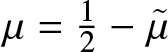 $\mu = \frac{1}{2} - \tilde{\mu}$ with
 $\tilde{\mu}$ defined near
 $0$. It follows from (5.1) that
 $\mathcal{H}_{\mu} = \mathcal{H}_{\rm aper}$ if
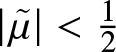 $|\tilde{\mu}| \lt \frac{1}{2}$, where
 $\mathcal{H}_{\rm aper}$ is the Hilbert transform acting on anti-periodic functions. Similarly, instead of (1.22), (1.23), (1.24) and (1.25), we have
 \begin{align*}
\mathcal{K}_{\mu} &= \mathcal{K}_{\rm aper} + i \tilde{\mu} \mathcal{H}_{\rm aper}, \\
\mathcal{M}_{\mu} &= \mathcal{M}_{\rm aper}, \quad
\mathcal{M}_{\mu}^* = \mathcal{M}^*_{\rm aper}, \\
\mathcal{L}_{\mu} &= \mathcal{L}_{\rm aper} + i \tilde{\mu} \mathcal{S}_{\rm aper},
\end{align*}
where the definitions of  $\mathcal{K}_{\rm aper}$,
 $\mathcal{M}_{\rm aper}$,
 $\mathcal{M}^*_{\rm aper}$ and
 $\mathcal{L}_{\rm aper}$ acting on antiperiodic functions follow from (1.3), (1.17) and (1.18), and
 \begin{equation*}
\mathcal{S}_{\rm aper} = c^2 \mathcal{H}_{\rm aper} - \eta \mathcal{H}_{\rm aper} - \mathcal{H}_{\rm aper} (\eta \; \cdot).
\end{equation*}
By using 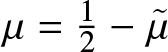 $\mu = \frac{1}{2} - \tilde{\mu}$ and the linear operators introduced above, we can rewrite the stability problem (1.27) in the equivalent form
 \begin{equation}
\left\{\begin{array}{ll}
(\mathcal{K}_{\rm aper} + i \tilde{\mu} \mathcal{H}_{\rm aper}) \hat{w} &= \lambda \mathcal{M}_{\rm aper} \hat{v}, \\
(\mathcal{L}_{\rm aper} + i \tilde{\mu} \mathcal{S}_{\rm aper}) \hat{v} &= \lambda (\mathcal{M}^*_{\rm aper} \hat{w}
- 2 c \mathcal{H}_{\rm aper} \hat{v}),
\end{array}
\right.
\end{equation}
where  $(\hat{v},\hat{w}) \in H^1_{\rm aper} \times H^1_{\rm aper}$ and
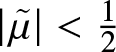 $|\tilde{\mu}| \lt \frac{1}{2}$.
The following theorem gives the criterion for the corresponding bifurcation. Compared to the case of the co-periodic perturbations in Sections 4, 6 and 7, the numerical coefficients of the normal form are not related to the conserved quantities computed at the travelling wave profile 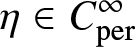 $\eta \in C^{\infty}_{\rm per}$. We also do not use Assumptions 1 and 2 since they determine the dimensions of the kernel and the generalized kernel of the spectral problem (1.19) for co-periodic perturbations in
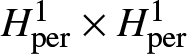 $H^1_{\rm per} \times H^1_{\rm per}$.
Theorem 3 Let Assumption 3 be true and define numerical coefficients  $\mathcal{A}_1$,
 $\mathcal{A}_2$ and
 $\mathcal{A}_3$ by (5.10) computed from the wave profile
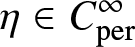 $\eta \in C^{\infty}_{\rm per}$ and the eigenfunction profile
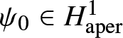 $\psi_0 \in H^1_{\rm aper}$. If
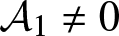 $\mathcal{A}_1 \neq 0$ and
 $\mathcal{A}_1 \mathcal{A}_3 + c^2 \mathcal{A}_2^2 \gt 0$, then there exist two spectral bands of the modulational stability problem (5.2) intersecting
 $\lambda = 0$, which are subsets of
 $i \mathbb{R}$ and non-degenerate.
Proof. To expand solutions of the spectral problem (5.2) near  $(\tilde{\mu},\lambda) = (0,0)$, we introduce the asymptotic expansion
 \begin{equation}
\tilde{\mu} = \epsilon \tilde{\mu}_1, \quad \lambda = \epsilon \lambda_1 + \mathcal{O}(\epsilon^2)
\end{equation}
and
 \begin{equation}
\left( \begin{array}{c} \hat{v} \\ \hat{w} \end{array} \right) = \left( \begin{array}{c} \psi_0 \\ 0 \end{array} \right) + \epsilon \left( \begin{array}{c} \hat{v}_1 \\ \hat{w}_1 \end{array} \right) + \epsilon^2 \left( \begin{array}{c} \hat{v}_2 \\ \hat{w}_2 \end{array} \right) + \mathcal{O}(\epsilon^3),
\end{equation}
where  $\epsilon$ is a small parameter,
 $\tilde{\mu}_1$ is fixed and the correction terms
 $(\hat{v}_1,\hat{w}_1)$ and
 $(\hat{v}_2,\hat{w}_2)$ at the
 $\mathcal{O}(\epsilon)$ and
 $\mathcal{O}(\epsilon^2)$ orders are to be computed in function space
 $H^1_{\rm aper} \times H^1_{\rm aper}$. The expansions (5.3) and (5.4) are justified due to the orthogonality of
 $\mathcal{S}_{\rm aper} \psi_0$ to
 $\psi_0$ in
 $L^2_{\rm aper}$ since
 $\mathcal{S}_{\rm aper}$ is skew-adjoint in
 $L^2_{\rm aper}$. This ensures that the term of the order of
 $\mathcal{O}(\mu^{1/2})$ in the expansion of
 $\lambda$ is identically zero and the next-order term is
 $\mathcal{O}(\mu)$, see Section 3.2.
 $\underline{\boldsymbol{\mathrm{Order}} \ \mathcal{O}(\epsilon)}$: We get the linear inhomogeneous system
 \begin{equation}
\left\{\begin{array}{ll}
\mathcal{K}_{\rm aper} \hat{w}_1 &= \lambda_1 \mathcal{M}_{\rm aper} \psi_0, \\
\mathcal{L}_{\rm aper} \hat{v}_1 &= - 2 c \lambda_1 \mathcal{H}_{\rm aper} \psi_0 + i \tilde{\mu}_1 \mathcal{S}_{\rm aper} \psi_0.
\end{array}
\right.
\end{equation}
Since  ${\rm Ker}(\mathcal{L}_{\rm aper}) = {\rm span}(\psi_0)$ in
 $H^1_{\rm aper}$ by Assumption 3, whereas
 $\mathcal{H}_{\rm aper}$ and
 $\mathcal{S}_{\rm aper}$ are skew-adjoint in
 $L^2_{\rm aper}$, the Fredholm condition is satisfied for the linear inhomogeneous system (5.5), and we obtain the solution in the form
 \begin{equation}
\left( \begin{array}{c} \hat{v}_1 \\ \hat{w}_1 \end{array} \right) = \lambda_1
\left( \begin{array}{c} -2c \mathcal{L}_{\rm aper}^{-1} \mathcal{H}_{\rm aper} \psi_0 \\ \mathcal{K}_{\rm aper}^{-1} \mathcal{M}_{\rm aper} \psi_0 \end{array} \right)
+ i \tilde{\mu}_1 \left( \begin{array}{c} \mathcal{L}_{\rm aper}^{-1} \mathcal{S}_{\rm aper} \psi_0 \\ 0 \end{array} \right).
\end{equation}
 $\underline{\boldsymbol{\mathrm{Order}} \ \mathcal{O}(\epsilon^2)}$: We get the linear inhomogeneous system
 \begin{equation}
\left\{\begin{array}{ll}
\mathcal{K}_{\rm aper} \hat{w}_2 &= \lambda_1 \mathcal{M}_{\rm aper} \hat{v}_1 + i \tilde{\mu}_1 \mathcal{H}_{\rm aper} \hat{w}_1, \\
\mathcal{L}_{\rm aper} \hat{v}_2 &= \lambda_1 \left( \mathcal{M}^*_{\rm aper} \hat{w}_1
- 2 c \mathcal{H}_{\rm aper} \hat{v}_1 \right) + i \tilde{\mu}_1 \mathcal{S}_{\rm aper} \hat{v}_1.
\end{array}
\right.
\end{equation}
By Fredholm’s theorem, there exists an anti-periodic solution of the linear inhomogeneous system (5.7) if and only if the following constraint is satisfied:
 \begin{equation}
\lambda_1 \langle \psi_0, \mathcal{M}^*_{\rm aper} \hat{w}_1
- 2 c \mathcal{H}_{\rm aper} \hat{v}_1 \rangle + i \tilde{\mu}_1 \langle \psi_0, \mathcal{S}_{\rm aper} \hat{v}_1 \rangle = 0.
\end{equation}
With the account of (5.6), the constraint (5.8) yields the following quadratic characteristic equation
 \begin{equation}
\lambda_1^2 \mathcal{A}_{1} + 2 i c \tilde{\mu}_1 \lambda_1 \mathcal{A}_{2} + \tilde{\mu}_1^2 \mathcal{A}_{3} = 0,
\end{equation}
with the following coefficients:
 \begin{equation}
\left\{\begin{array}{l}
\mathcal{A}_1 = \langle \mathcal{M}_{\rm aper} \psi_0, \mathcal{K}_{\rm aper}^{-1} \mathcal{M}_{\rm aper} \psi_0 \rangle - 4 c^2 \langle \mathcal{H}_{\rm aper} \psi_0, \mathcal{L}_{\rm aper}^{-1} \mathcal{H}_{\rm aper} \psi_0 \rangle, \\
\mathcal{A}_2 = \langle \mathcal{H}_{\rm aper} \psi_0, \mathcal{L}_{\rm aper}^{-1} \mathcal{S}_{\rm aper} \psi_0 \rangle + \langle \mathcal{S}_{\rm aper} \psi_0, \mathcal{L}_{\rm aper}^{-1} \mathcal{H}_{\rm aper} \psi_0 \rangle, \\
\mathcal{A}_3 = \langle \mathcal{S}_{\rm aper} \psi_0, \mathcal{L}_{\rm aper}^{-1} \mathcal{S}_{\rm aper} \psi_0 \rangle, \end{array} \right.
\end{equation}
where we have used the skew-adjointness of  $\mathcal{H}_{\rm aper}$ and
 $\mathcal{S}_{\rm aper}$ in
 $L^2_{\rm per}$.
If 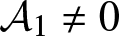 $\mathcal{A}_1 \neq 0$, two solutions of the quadratic equation (5.9) are given by
 \begin{equation}
\lambda_1^{\pm}(\tilde{\mu}_1) = - \frac{ic \tilde{\mu}_1 \mathcal{A}_2}{\mathcal{A}_1} \pm \frac{i \tilde{\mu}_1}{\mathcal{A}_1} \sqrt{\mathcal{A}_1 \mathcal{A}_3 + c^2 \mathcal{A}_2^2},
\end{equation}
with the discriminant
 \begin{align*}
\mathcal{A}_1 \mathcal{A}_3 + c^2 \mathcal{A}_2^2 &= \langle \mathcal{M}_{\rm aper} \psi_0, \mathcal{K}_{\rm aper}^{-1} \mathcal{M}_{\rm aper} \psi_0 \rangle \langle \mathcal{S}_{\rm aper} \psi_0, \mathcal{L}_{\rm aper}^{-1} \mathcal{S}_{\rm aper} \psi_0 \rangle \\
& \quad + 4 c^2 \left[ |\langle \mathcal{H}_{\rm aper} \psi_0, \mathcal{L}_{\rm aper}^{-1} \mathcal{S}_{\rm aper} \psi_0 \rangle|^2 \right. \\
& \left. \qquad - \langle \mathcal{H}_{\rm aper} \psi_0, \mathcal{L}_{\rm aper}^{-1} \mathcal{H}_{\rm aper} \psi_0 \rangle \langle \mathcal{S}_{\rm aper} \psi_0, \mathcal{L}_{\rm aper}^{-1} \mathcal{S}_{\rm aper} \psi_0 \rangle
\right].
\end{align*}
If 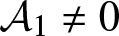 $\mathcal{A}_1 \neq 0$ and
 $\mathcal{A}_1 \mathcal{A}_3 + c^2 \mathcal{A}_2^2 \gt 0$, then
 $\lambda_1^{\pm}(\tilde{\mu}_1) \in i \mathbb{R}$ for
 $\tilde{\mu}_1 \in \mathbb{R}$ and
 $\lambda_1^+(\tilde{\mu}_1) \neq \lambda_1^-(\tilde{\mu}_1)$ for
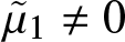 $\tilde{\mu}_1 \neq 0$. Persistence of the two spectral bands crossing
 $\lambda = 0$ on
 $i \mathbb{R}$ in the asymptotic expansions (5.3) and (5.4) follows from the Hamiltonian symmetry of Lemma 2.
5.2. Normal form of the bifurcation
The bifurcation induced by Assumption 3 is the period-doubling (subharmonic) bifurcation [Reference Buffoni, Dancer and Toland11]. In addition, it is also related to the stability bifurcation for the spectral problem (5.2) for  $\tilde{\mu} = 0$ in the space of antiperiodic perturbations in
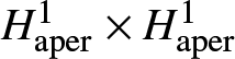 $H^1_{\rm aper} \times H^1_{\rm aper}$. The bifurcation is induced by the small eigenvalue of the linearized operator
 $\mathcal{L}_{\rm aper}$ which crosses
 $0$ as
 $c$ changes through the bifurcation point.
The following lemma describes the transformation of the small eigenvalue of  $\mathcal{L}_{\rm aper}$.
Lemma 6. Let 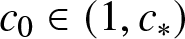 $c_0 \in (1,c_*)$ be the bifurcation point, under which Assumption 3 holds with the
 $L^2$-normalized eigenfunction
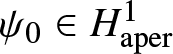 $\psi_0 \in H^1_{\rm aper}$. There exists an eigenvalue
 $\Lambda(c)$ of
 $\mathcal{L}_{\rm aper}$ with the
 $L^2$-normalized eigenfunction
 $\psi(\cdot,c) \in H^1_{\rm aper}$, which are
 $C^{\infty}$ functions of
 $c$ at
 $c_0$ satisfying
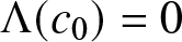 $\Lambda(c_0) = 0$ and
 $\psi(\cdot,c_0) = \psi_0$.
Proof. By the theory in [Reference Buffoni, Dancer and Toland11], the wave profile 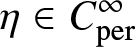 $\eta \in C^{\infty}_{\rm per}$ satisfies Assumption 1 if
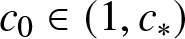 $c_0 \in (1,c_*)$ is the subharmonic bifurcation point, for which Assumption 3 holds. Hence, the wave profile is continuously differentiable in
 $c$ at
 $c_0$ by Lemma 3. By the bootstrapping argument, it is actually
 $C^{\infty}$, so that the linearized operator
 $\mathcal{L}_{\rm aper}$ has smooth coefficients in
 $c$ at
 $c_0$ and we can write
 \begin{equation}
\mathcal{L}_{\rm aper} = \mathcal{L}_{\rm aper}^{(0)} + (c-c_0) \mathcal{L}_{\rm aper}^{(1)} + \mathcal{O}((c-c_0)^2),
\end{equation}
where
 \begin{align*}
\mathcal{L}_{\rm aper}^{(0)} &= c_0^2 \mathcal{K}_{\rm aper} - (1 + \mathcal{K} \eta) - \eta \mathcal{K}_{\rm aper} - \mathcal{K}_{\rm aper} (\eta \; \cdot ), \\
\mathcal{L}_{\rm aper}^{(1)} &= 2 c_0 \mathcal{K}_{\rm aper} - \left( \mathcal{K} \partial_c \eta |_{c = c_0} \right) - \partial_c \eta |_{c = c_0} \mathcal{K}_{\rm aper} - \mathcal{K}_{\rm aper} \left( \partial_c \eta |_{c = c_0} \; \cdot \right).
\end{align*}
As follows from the analytic perturbation theory [Reference Hinch25], the eigenvalue–eigenfunction pair  $(\Lambda,\psi)$ of
 $\mathcal{L}_{\rm aper}$ is also smooth near
 $(0,\psi_0)$, since the kernel of
 $\mathcal{L}_{\rm aper}$ is simple by Assumption 3. This gives the assertion of the lemma.
Remark 12. By using the decomposition
 \begin{equation*}
\Lambda(c) = \Lambda'(c_0) (c-c_0) + \mathcal{O}((c-c_0)^2), \quad
\psi(\cdot,c) = \psi_0 + \psi_1 (c - c_0) + \mathcal{O}((c-c_0)^2)
\end{equation*}
in the solutions of  $\mathcal{L}_{\rm aper} \psi(\cdot,c) = \Lambda(c) \psi(\cdot,c)$, we obtain the linear inhomogeneous equation for
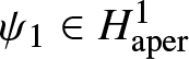 $\psi_1 \in H^1_{\rm aper}$:
 \begin{equation*}
\mathcal{L}_{\rm aper}^{(0)} \psi_1 + \mathcal{L}_{\rm aper}^{(1)} \psi_0 = \Lambda'(c_0) \psi_0.
\end{equation*}
Projecting this equation to  $\psi_0$ yields the Fredholm condition for the existence of
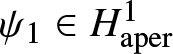 $\psi_1 \in H^1_{\rm aper}$:
 \begin{equation}
\Lambda'(c_0) = \frac{\langle \mathcal{L}_{\rm aper}^{(1)} \psi_0, \psi_0 \rangle}{\langle \psi_0,\psi_0 \rangle},
\end{equation}
which is generally nonzero.
The following theorem gives the normal form for the stability bifurcation in the spectral problem (5.2).
Theorem 4 Under the assumptions of Theorem 3, let 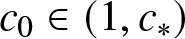 $c_0 \in (1,c_*)$ be the root of
 $\Lambda(c)$, where
 $\Lambda(c)$ is the eigenvalue of
 $\mathcal{L}_{\rm aper}$ in Lemma 6. Assume that
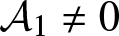 $\mathcal{A}_1 \neq 0$ and
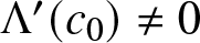 $\Lambda'(c_0) \neq 0$ in (5.10) and (5.13). The two spectral bands of the modulational stability problem (5.2) near
 $\lambda = 0$ in Theorem 3 are obtained from roots of the characteristic equation
 \begin{equation}
\lambda^2\mathcal{A}_{1} + 2 i c_0 \tilde{\mu} \lambda \mathcal{A}_{2} + \tilde{\mu}^2 \mathcal{A}_{3}
- \Lambda'(c_0) (c-c_0) \| \psi_0 \|^2_{L^2} = \mathcal{O}\left( |\tilde{\mu}|^3 \right),
\end{equation}
where the asymptotic balance is justified if  $c - c_0 = \mathcal{O}( \tilde{\mu}^2)$.
Proof. We combine the asymptotic expansions (5.3), (5.4) and (5.12) at the asymptotic balance  $c - c_0 = \mathcal{O}(\tilde{\mu}^2)$. To incorporate the balance, we write
 \begin{equation*}
c = c_0 + \epsilon^2 c_2 + \mathcal{O}(\epsilon^3),
\end{equation*}
where  $c_2$ is fixed. We get the same solution (5.6) with
 $c = c_0$ at the order
 $\mathcal{O}(\epsilon)$ and we get the following modification of the linear inhomogeneous system (5.7) at the order
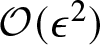 $\mathcal{O}(\epsilon^2)$:
 \begin{equation}
\left\{\begin{array}{ll}
\mathcal{K}_{\rm aper} \hat{w}_2 &= \lambda_1 \mathcal{M}_{\rm aper} \hat{v}_1 + i \tilde{\mu}_1 \mathcal{H}_{\rm aper} \hat{w}_1, \\
\mathcal{L}_{\rm aper}^{(0)} \hat{v}_2 + c_2 \mathcal{L}_{\rm aper}^{(1)} \psi_0 &= \lambda_1 \left( \mathcal{M}^*_{\rm aper} \hat{w}_1
- 2 c_0 \mathcal{H}_{\rm aper} \hat{v}_1 \right) + i \tilde{\mu}_1 \mathcal{S}_{\rm aper} \hat{v}_1.
\end{array}
\right.
\end{equation}
By Fredholm’s theorem, there exists a periodic solution of the linear inhomogeneous system (5.15) if and only if the following constraint is satisfied:
 \begin{equation}
\lambda_1 \langle \psi_0, \mathcal{M}^*_{\rm aper} \hat{w}_1
- 2 c_0 \mathcal{H}_{\rm aper} \hat{v}_1 \rangle + i \tilde{\mu}_1 \langle \psi_0, \mathcal{S}_{\rm aper} \hat{v}_1 \rangle = c_2 \langle \psi_0, \mathcal{L}_{\rm aper}^{(1)} \psi_0 \rangle.
\end{equation}
With the account of (5.9) and (5.13), the constraint (5.16) yields the following quadratic characteristic equation
 \begin{equation}
\lambda_1^2 \mathcal{A}_{1} + 2 i c_0 \tilde{\mu}_1 \lambda_1 \mathcal{A}_{2} + \tilde{\mu}_1^2 \mathcal{A}_{3} = c_2 \Lambda'(c_0) \| \psi_0 \|^2_{L^2},
\end{equation}
where the coefficients  $\mathcal{A}_{1,2,3}$ are defined by (5.10). Multiplying (5.17) by
 $\epsilon^2$, keeping in mind the remainder term of the order
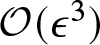 $\mathcal{O}(\epsilon^3)$, and returning to the original variables
 $\mu$,
 $\lambda$ and
 $c$, we obtain (5.14).
Remark 13. If 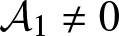 $\mathcal{A}_1 \neq 0$ and
 $\mathcal{A}_1 \mathcal{A}_3 + c_0^2 \mathcal{A}_2^2 \gt 0$, then
 $\lambda^2\mathcal{A}_{1} + 2 i c_0 \tilde{\mu} \lambda \mathcal{A}_{2} + \tilde{\mu}^2 \mathcal{A}_{3} = 0$ has two roots
 $\lambda^{\pm}(\tilde{\mu}) \in i \mathbb{R}$ such that
 $\lambda^+(\tilde{\mu}) \neq \lambda^-(\tilde{\mu})$ for
 $\tilde{\mu} \neq 0$, see (5.11). If
 ${\rm sgn}(\Lambda'(c_0)) = {\rm sgn}(\mathcal{A}_1)$, then the spectral problem (5.2) with
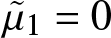 $\tilde{\mu}_1 = 0$ admits two real eigenvalues for
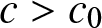 $c \gt c_0$ and two purely imaginary eigenvalues for
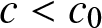 $c \lt c_0$ near the origin. Rewriting (5.14) as
 \begin{equation*}
\left( \lambda + \frac{i c_0 \tilde{\mu} \mathcal{A}_2}{\mathcal{A}_1} \right)^2 +
\tilde{\mu}^2 \frac{\mathcal{A}_1 \mathcal{A}_{3} + c^2 \mathcal{A}_2^2}{\mathcal{A}_1^2}
- \frac{\Lambda'(c_0) \| \psi_0 \|^2_{L^2}}{\mathcal{A}_1} (c-c_0) = \mathcal{O}\left( |\tilde{\mu}|^3 \right),
\end{equation*}
we can see that the roots define two spectral bands, which are subsets of  $i \mathbb{R}$ and non-degenerate for
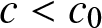 $c \lt c_0$. Compared to the case of
 $c = c_0$, these two spectral bands do not intersect
 $\lambda = 0$ for
 $c \lt c_0$. If
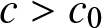 $c \gt c_0$, the roots define a new circular band around the origin, the radius of which grows as
 $c$ deviates from
 $c_0$.
5.3. Numerical results
The criterion for the ellipse bifurcation is a zero of  $\Lambda(c)$, the eigenvalue of
 $\mathcal{L}_{\rm aper}$ for an anti-periodic eigenfunction (see red circles in Figure 3). The corresponding steepness
 $s_0$ and speed
 $c_0$ for the first two zeros of
 $\Lambda$ are recorded in Table 3, where we also show the values of
 $\mathcal{A}_1$,
 $\mathcal{A}_2$,
 $\mathcal{A}_1 \mathcal{A}_3 + c_0^2 \mathcal{A}_2^2$ and
 $\Lambda'(c_0)$ in the normal form (5.14).
Parameters of the first two ellipse bifurcations

Table 3 Long description
Two rows list parameter values across columns labeled s0, c0, A1, A2, a combined term involving A1, A2, A3 and c squared, and Lambda prime at c0. Row 1 has s0 0.12890310 and c0 1.08414013, with A1 minus 4.7027, A2 1.3601, the combined term 0.99841, and Lambda prime at c0 minus 28.87. Row 2 has s0 0.14048675 and c0 1.09238125, with A1 minus 4.4533, A2 1.2802, the combined term 0.89648, and Lambda prime at c0 2391.7. From row 1 to row 2, s0 and c0 increase, A1 becomes less negative, and A2 decreases. Over the same change, the combined term decreases, while Lambda prime at c0 changes sign and increases in magnitude.
We note that  $\mathcal{A}_1 \neq 0$ and
 $\mathcal{A}_1 \mathcal{A}_3 + c^2 \mathcal{A}_2^2 \gt 0$ so that the splitting of two spectral bands near
 $\lambda = 0$ occurs similarly to the description in Remark 13. The only difference is that the mapping
 $s \mapsto c(s)$ is increasing at the first ellipse bifurcation and decreasing at the second ellipse bifurcation. Therefore, the values of
 $\Lambda'(c_0)$ change the sign in between the two bifurcations, which correspond to the real eigenvalues of the spectral problem (5.2) with
 $\tilde{\mu}_1 = 0$ for
 $c \gt c_0$ for the first bifurcation and
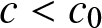 $c \lt c_0$ for the second bifurcation, both regions correspond to the steepness
 $s$ above the critical steepness
 $s_0$.
There are two equivalent ways to determine the eigenfunction  $\psi_0 \in H^1_{\rm aper}$. The first method is to solve the eigenvalue problem for
 $\mathcal{L}_{\rm mu}$ using Floquet multiplier with
 $\mu = \frac{1}{2}$. The second is to extend the interval for
 $u$ to
 $[0,4\pi]$, and seek the unique odd
 $4\pi$-periodic eigenfunction of
 $\mathcal{L}_{\rm aper}$. We chose to follow the second route, where we also use the symmetry of Babenko’s equation (1.11): if
 $\eta \in C^{\infty}_{\rm per}$ is a solution for speed
 $c$, then
 $\tilde{\eta}(u) = \frac{1}{2} \eta(2u)$ is also a solution for speed
 $\tilde{c} = \frac{c}{\sqrt{2}}$. This scaling symmetry allows us to recast a
 $4\pi$-periodic function back to a
 $2\pi$-periodic function. We obtain
 $\psi_0$ from the shift-and-invert numerical method applied to
 $\mathcal{L}_{\rm aper}$, see [Reference Dyachenko and Semenova24]. The value of
 $\Lambda'(c_0)$ is determined from the equation (5.13). After
 $\psi_0 \in H^1_{\rm aper}$ is found, we compute the three inner products
 $A_{1,2,3}$ in relations (5.10), with the inverse operator
 $\mathcal{L}^{-1}$ applied via the MINRES method.
Figures 11 and 12 show the instability bands of the spectral problem (1.27) near the origin in the spectral  $\lambda$-plane obtained numerically (blue dots). The three panels in each figure correspond to three consequent values of steepness before, at, and after the critical steepness, for which
 $\Lambda(c_0) = 0$. The theoretical curves obtained from the normal form (5.14) are shown in red colour. A good agreement between the spectral bands given by the normal form (5.14) and the numerical approximations of the stability spectra is evident for the first two cycles of bifurcations.
The first instance of the ellipse bifurcation, which corresponds to panels (e)–(g) of Figure 1 zoomed near the origin in the  $\lambda$-plane. The spectral bands remain on
 $i \mathbb{R}$ for
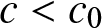 $c \lt c_0$ (left panel), remain on
 $i \mathbb{R}$ and intersect the origin for
 $c = c_0$ (middle panel), and form a circular band around the origin for
 $c \gt c_0$ (right panel), where
 $c_0 \approx 1.08414013$ is found from the root of
 $\Lambda$. The dashed lines show the approximations obtained from the normal form (5.14).

The same as Figure 11 but for the second instance of the ellipse bifurcation, which happens when 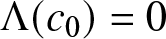 $\Lambda(c_0) = 0$ for
 $c_0 \approx 1.09238125$.

6. Reconnection of figure-
$\infty$ bands

The corresponding bifurcation is seen in panels (j)–(l) of Figure 1. For simplicity, it can be called the figure- $\infty$ bifurcation. Before the bifurcation [panel (j)], the instability band surrounding the origin has a peanut shape. At the bifurcation [panel (k)], the instability band reconnects at the origin and exhibits the figure-
 $\infty$ shape. After the bifurcation [panel (l)], the figure-
 $\infty$ band breaks into two instability bubbles along the real axis.
Section 6.1 develops the criterion and the normal form for this bifurcation. Section 6.2 describes numerical approximations of the coefficients of the normal form, from which we are able to reproduce the bifurcation pattern seen in panels (j)–(l) of Figure 1.
6.1. Criterion and the normal form of the bifurcation
This bifurcation is due to the zero-eigenvalue bifurcation in the spectral problem (1.19) for co-periodic perturbations, which was considered in our previous work [Reference Dyachenko and Pelinovsky20]. The geometric multiplicity of the zero eigenvalue is controlled by Assumption 1, which is still considered to be true. However, the algebraic multiplicity of the zero eigenvalue is increased from four to six, since Assumption 2 is no longer considered to be true. Hence, we replace Assumption 2 with the opposite non-generic assumption.
Assumption 4. For the given value of 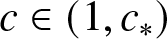 $c \in (1,c_*)$, we have
 $\mathcal{P}'(c) = 0$.
Because of Assumption 4, the generalized kernel of the spectral problem (1.27) for  $\mu = 0$ is at least six-dimensional. It was shown in [Reference Dyachenko and Pelinovsky20] that it is exactly six-dimensional if
 $\mathcal{B} \neq 0$, where the numerical coefficient
 $\mathcal{B}$ is defined by (6.14).
The following theorem gives the criterion for the corresponding bifurcation.
Theorem 5 Let Assumptions 1 and 4 be true and assume that  $\mathcal{B} \neq 0$ in (6.14). There exist six spectral bands of the modulational stability problem (1.27) intersecting
 $\lambda = 0$. Two spectral bands cross the origin along the straight lines in all four complex quadrants of the complex
 $\lambda$-plane, and four spectral bands are subsets of
 $i \mathbb{R}$ and non-degenerate.
Proof. We revisit the proof of Theorem 1 after replacing Assumption 2 with Assumption 4. If  $\mathcal{P}'(c) = 0$, then the characteristic equation (4.20) fails because the coefficient in front of
 $\lambda_1^2$ vanishes. If
 $\mathcal{B} \neq 0$ in (6.14), then the characteristic equation can be extended to the next term of
 $\lambda_1^4$. According to Section 3.3, we get the splitting formula for eigenvalues in the form (3.22), where three eigenvalues with
 $\lambda = \mathcal{O}(\mu^{1/3})$ and one eigenvalue with
 $\lambda = \mathcal{O}(\mu)$ are obtained in the subspace
 $(a_1,a_2) = (1,0)$ and two eigenvalues with
 $\lambda = \mathcal{O}(\mu^{1/2})$ are obtained in the subspace
 $(a_1,a_2) = (0,1)$. Since the two balances are different, we can still consider these two subspaces separately from each other, similarly to the proof of Theorem 1, with two different expansions near
 $(\mu,\lambda) = (0,0)$.
 $\underline{\boldsymbol{\mathrm{Subspace}}(a_1,a_2) = (1,0)}$: We introduce the asymptotic expansions
 \begin{equation}
\mu = \epsilon^3 \mu_3, \quad \lambda = \epsilon \lambda_1 + \mathcal{O}(\epsilon^2)
\end{equation}
and
 \begin{equation}
\left( \begin{array}{c} \hat{v} \\ \hat{w} \end{array} \right) = \left( \begin{array}{c} \eta' \\ 0 \end{array} \right) + \epsilon \left( \begin{array}{c} \hat{v}_1 \\ \hat{w}_1 \end{array} \right) + \epsilon^2 \left( \begin{array}{c} \hat{v}_2 \\ \hat{w}_2 \end{array} \right) + \epsilon^3 \left( \begin{array}{c} \hat{v}_3 \\ \hat{w}_3 \end{array} \right) + \epsilon^4 \left( \begin{array}{c} \hat{v}_4 \\ \hat{w}_4 \end{array} \right) + \mathcal{O}(\epsilon^5),
\end{equation}
where  $\epsilon \gt 0$ is a small parameter,
 $\mu_3 \neq 0$ is fixed and the correction terms up to the order of
 $\mathcal{O}(\epsilon^4)$ are to be computed recursively in function space
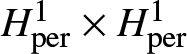 $H^1_{\rm per} \times H^1_{\rm per}$.
 $\underline{\boldsymbol{\mathrm{Order}} \ \mathcal{O}(\epsilon)}$: We get the linear inhomogeneous system (4.9) without the
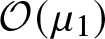 $\mathcal{O}(\mu_1)$ terms. Hence, instead of the solution (4.11), we obtain the truncated solution
 \begin{equation}
\left( \begin{array}{c} \hat{v}_1 \\ \hat{w}_1 \end{array} \right) = \lambda_1
\left[ \left( \begin{array}{c} -\partial_c \eta \\ \mathcal{H} \eta \end{array} \right) \pm i \langle 1, \partial_c \eta \rangle
\left( \begin{array}{c} \eta' \\ -c \end{array} \right)
\right],
\end{equation}
where no projections to  $(\eta',0)^T$ and
 $(0,1)^T$ are needed to satisfy the Fredholm conditions in the higher orders.
 $\underline{\boldsymbol{\mathrm{Order}} \ \mathcal{O}(\epsilon^2)}$: We get the linear inhomogeneous system (4.12) without the
 $\mathcal{O}(\mu_1)$ terms. Moreover, the second term in (6.3) cancels all the plus/minus projection terms due to Lemma 5. By using (4.15) and
 $\mathcal{P}'(c) = 0$, we confirm that the solvability constraints are satisfied and there exists a periodic solution of the linear inhomogeneous system in the form
 \begin{equation}
\left( \begin{array}{c} \hat{v}_2 \\ \hat{w}_2 \end{array} \right) = \lambda_1^2 \left( \begin{array}{c} \tilde{v}_2 \\ \tilde{w}_2 \end{array} \right) + a \left( \begin{array}{c} 0 \\ 1 \end{array} \right),
\end{equation}
where  $a \in \mathbb{R}$ is arbitrary at this order, the projection to
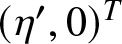 $(\eta',0)^T$ is not included since the eigenfunctions are defined up to the arbitrary scalar multiplication in (6.2), and
 $(\tilde{v}_2,\tilde{w}_2) \in H^1_{\rm per} \times H^1_{\rm per}$ is uniquely determined from solution of the linear inhomogeneous system
 \begin{equation}
\left\{\begin{array}{ll}
\mathcal{K} \tilde{w}_2 &= - \mathcal{M} \partial_c \eta, \\
\mathcal{L} \tilde{v}_2 &= \mathcal{M}^* \mathcal{H}\eta + 2 c \mathcal{H} \partial_c \eta,
\end{array}
\right.
\end{equation}
under the orthogonality conditions  $\langle 1, \tilde{w}_2 \rangle = \langle \eta', \tilde{v}_2 \rangle = 0$. Since the linearized operators in (6.5) are parity-preserving, the functions
 $\tilde{v}_2$ and
 $\tilde{w}_2$ are spatially odd and even in
 $u$, respectively.
 $\underline{\boldsymbol{\mathrm{Order}} \ \mathcal{O}(\epsilon^3)}$: We get the linear inhomogeneous system
 \begin{equation}
\left\{\begin{array}{ll}
\mathcal{K} \hat{w}_3 &= \lambda_1 \mathcal{M} \hat{v}_2, \\
\mathcal{L} \hat{v}_3 &= \lambda_1 \left( \mathcal{M}^* \hat{w}_2 - 2 c \mathcal{H} \hat{v}_2 \right) + i \mu_3 \mathcal{L}_{\pm} \eta'.
\end{array}
\right.
\end{equation}
By using (4.2), (4.10), (4.11) and (6.4), there exists a periodic solution to (6.6) in the form
 \begin{align}\left( \begin{array}{c} \hat{v}_3 \\ \hat{w}_3 \end{array} \right) &= \lambda_1^3
\left[ \left( \begin{array}{c} \tilde{v}_3 \\ \tilde{w}_3 \end{array} \right) \mp i \langle 1, \tilde{v}_3 \rangle
\left( \begin{array}{c} \eta' \\ -c \end{array} \right)
\right]
+ i \mu_3 \left( \begin{array}{c} \Upsilon \\ 0 \end{array} \right) \notag \\
& \qquad \qquad
+ a \lambda_1 \left[
\left( \begin{array}{c} -1 \\ 0 \end{array} \right) \pm i \left( \begin{array}{c} \eta' \\ -c \end{array} \right) \right],\end{align}
where projections to  $(\eta',0)^T$ and
 $(0,1)^T$ are not included since the eigenfunctions are defined up to the arbitrary scalar multiplication in (6.2) and (6.4), and
 $(\tilde{v}_3,\tilde{w}_3) \in H^1_{\rm per} \times H^1_{\rm per}$ is uniquely determined from solution of the linear inhomogeneous system
 \begin{equation}
\left\{\begin{array}{ll}
\mathcal{K} \tilde{w}_3 &= \mathcal{M} \tilde{v}_2, \\
\mathcal{L} \tilde{v}_3 &= \mathcal{M}^* \tilde{w}_2 - 2 c \mathcal{H} \tilde{v}_2,
\end{array}
\right.
\end{equation}
under the orthogonality conditions  $\langle 1, \tilde{w}_3 \rangle = \langle \eta', \tilde{v}_3 \rangle = 0$. Since the linearized operators in (6.8) are parity-preserving, the functions
 $\tilde{v}_3$ and
 $\tilde{w}_3$ are spatially even and odd in
 $u$, respectively. A projection term was added in (6.7) due to the representation (2.11) since
 $\langle 1, \tilde{v}_3 \rangle \neq 0$ generally.
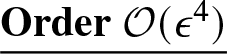 $\underline{\boldsymbol{\mathrm{Order}} \ \mathcal{O}(\epsilon^4)}$: We get the linear inhomogeneous system
 \begin{equation}
\left\{\begin{array}{ll}
\mathcal{K} \hat{w}_4 &= \lambda_1 \left( \mathcal{M} \hat{v}_3 \pm i \langle 1, \hat{v}_3 \rangle \eta' \right) + i \mu_3 \left( \mathcal{H} \hat{w}_1 \pm i \langle 1, \hat{w}_1 \rangle \right), \\
\mathcal{L} \hat{v}_4 &= \lambda_1 \left( \mathcal{M}^* \hat{w}_3
- 2 c \mathcal{H} \hat{v}_3 \mp i \langle \eta', \hat{w}_3 \rangle \mp 2 c i \langle 1, \hat{v}_3 \rangle \right) + i \mu_3 \mathcal{L}_{\pm} \hat{v}_1.
\end{array}
\right.
\end{equation}
By Fredholm’s theorem, there exists a periodic solution of the linear inhomogeneous system (6.9) if and only if the two constraints are satisfied:
 \begin{equation}
\lambda_1 \langle 1, \mathcal{M} \hat{v}_3 \rangle \mp \mu_3 \langle 1, \hat{w}_1 \rangle = 0,
\end{equation}
 \begin{equation}
\lambda_1 \langle \eta', \mathcal{M}^* \hat{w}_3
- 2 c \mathcal{H} \hat{v}_3 \rangle + i \mu_3 \langle \eta', \mathcal{L}_{\pm} \hat{v}_1 \rangle = 0.
\end{equation}
Since  $\mathcal{M}^* 1 = 1 + 2 \mathcal{K}\eta$, the first equation (6.10) yields due to (6.3) and (6.7):
 \begin{equation*}
\lambda_1^4 \langle (1+2\mathcal{K} \eta), \tilde{v}_3 \rangle +
i \mu_3 \lambda_1 \langle (1 + 2 \mathcal{K} \eta), \Upsilon \rangle - a \lambda_1^2 + i c \mu_3 \lambda_1 \langle 1, \partial_c \eta \rangle = 0.
\end{equation*}
This equation defines  $a$ uniquely as
 \begin{equation}
a = \lambda_1^2 \langle (1+2\mathcal{K} \eta), \tilde{v}_3 \rangle,
\end{equation}
where the term of  $\mu_3 \lambda_1^{-1}$ has zero coefficients due to (4.17) and (4.18) with
 $\mathcal{P}'(c) = 0$. Similarly, the second equation (6.11) yields due to (6.3) and (6.7):
 \begin{equation}
\lambda_1^4 \left[ \langle \eta', \tilde{w}_3 \rangle - 2 c \langle \mathcal{K} \eta, \tilde{v}_3 \rangle \right] - i \mu_3 \lambda_1 \left[ \langle \eta, \partial_c \eta \rangle + 2 c \langle \mathcal{K}\eta, \Upsilon \rangle \right] = 0,
\end{equation}
We note again that the numerical coefficient  $a$ given by (6.12) does not contribute to the computation of the characteristic equation (6.13). By using the numerical coefficient
 $\mathcal{B}$ given by
 \begin{equation}
\mathcal{B} := \langle \eta', \tilde{w}_3 \rangle - 2 c \langle \mathcal{K} \eta, \tilde{v}_3 \rangle,
\end{equation}
we obtain the quartic characteristic equation from (6.13):
 \begin{equation}
\lambda_1^4 \mathcal{B} - i \mu_3 \lambda_1 \mathcal{N}'(c) = 0.
\end{equation}
Due to the second identity in (2.9), if  $\mathcal{P}'(c) = 0$, then
 $\mathcal{N}'(c) = -5 \mathcal{P}(c) \lt 0$. Since
 $\mathcal{B} \neq 0$ is assumed, the quartic equation admits three nonzero solutions
 $\lambda_1^{(1,2,3)}(\mu_3)$ given by
 \begin{equation*}
\lambda_1^{(j)}(\mu_3) = (\mu_3 \mathcal{B}^{-1} \mathcal{N}'(c))^{1/3} e^{\frac{ij\pi}{6}}, \quad j = 1,2,3,
\end{equation*}
two of which give two straight lines in all four quadrants of the complex  $\lambda$-plane and one gives the vertical segment on
 $i \mathbb{R}$. The fourth root in (6.15) is zero at this order. According to the analysis in Section 3.3, the fourth root is of the order
 $\lambda = \mathcal{O}(\mu)$.
For fixed  $\mu_3 \neq 0$, the three eigenvalues
 $\lambda_1^{(1,2,3)}$ are distinct. The eigenvalue on
 $i \mathbb{R}$ remains on
 $i \mathbb{R}$ due to the Hamiltonian symmetry of Lemma 2. The other two simple eigenvalues are complex-valued and remain in the corresponding quadrants of the complex
 $\lambda$-plane under the perturbation terms in the asymptotic expansions (6.1) and (6.2). The fourth eigenvalue of the order of
 $\lambda = \mathcal{O}(\mu)$ is simple and belongs to
 $i \mathbb{R}$ due to Hamiltonian symmetry.
 $\underline{\boldsymbol{\mathrm{Subspace}}(a_1,a_2) = (0,1)}$: We use the same asymptotic expansions (4.22) and (4.23) as in the proof of Theorem 1. The same computations give two roots
 $\lambda_1^{\pm}(\mu_2) = \pm \sqrt{|\mu_2|}$ with two roots on
 $i \mathbb{R}$, which remain on
 $i \mathbb{R}$ under the perturbation terms due to the Hamiltonian symmetry of Lemma 2.
Remark 14. Let  $c = c_0$ be the root of
 $\mathcal{P}'(c)$ as in Assumption 4 and assume
 $\mathcal{P}''(c_0) \neq 0$. Continuation of the characteristic equation (6.15) for
 $c$ close to
 $c_0$ yields the normal form for the corresponding bifurcation, see [Reference Dyachenko and Pelinovsky20],
 \begin{equation}
\lambda^4 \mathcal{B} - i \mu \lambda \mathcal{N}'(c_0) + \lambda^2 \mathcal{P}''(c_0) (c - c_0) = \mathcal{O}(\mu^2),
\end{equation}
where  $c - c_0 = \mathcal{O}(|\mu|^{2/3})$ at the leading-order balance. For any
 $c \neq c_0$, there exist two roots
 $\lambda$ of (6.16) on
 $i \mathbb{R}$. Indeed, the transformation
 $\lambda = i \omega$ yields
 \begin{equation}
\omega^4 \mathcal{B} + \mu \omega \mathcal{N}'(c_0) - \omega^2 \mathcal{P}''(c_0) (c - c_0) = \mathcal{O}(\mu^2),
\end{equation}
where the coefficients in the remainder term are real-valued due to the Hamiltonian symmetry of Lemma 2. There exists two roots  $\omega$ of (6.17) on
 $\mathbb{R}$: one root is of the order
 $\mathcal{O}(|\mu|^{1/3})$ and the other root is of the order
 $\mathcal{O}(\mu)$ for any
 $c \neq c_0$. These two real roots for
 $\omega$ define two roots
 $\lambda$ of (6.16) on
 $i\mathbb{R}$. The other two roots of (6.16) are complex-valued for any
 $c \neq c_0$.
6.2. Numerical results
The criterion for the bifurcation is a zero of  $\mathcal{P}'(c)$, which is equivalent to a zero of
 $\mathcal{H}'(c)$ due to (2.9). The chain of eigenfunctions
 $(\tilde v_2, \tilde w_2)$ and
 $(\tilde v_3, \tilde w_3)$ defined by the linear inhomogeneous equations (6.5) and (6.8) only exists at
 $\mathcal{H}'(c)=0$. It follows from Figure 2 that there exists exactly one such zero of
 $\mathcal{H}'(c)$ (red solid line) between each turning point of speed with respect to steepness where
 $c'(s) = 0$ (vertical lines). The corresponding steepness
 $s_0$ and speed
 $c_0$ for the first two zeros of
 $\mathcal{H}'(c)$ are recorded in Table 4, where we also show the coefficients
 $\mathcal{P}''(c_0)$,
 $\mathcal{B}$ and
 $\mathcal{N}'(c_0)$ of the normal form (6.16). We note that
 $\mathcal{B} \gt 0$ and the sign of
 $\mathcal{P}''(c_0)$ alternates between the two bifurcations. In both cases, this leads to new unstable (real) eigenvalues of the spectral problem (1.19) in
 $L^2_{\rm per}$ in the direction of increasing steepness
 $s$ past the critical steepness
 $s_0$, see [Reference Dyachenko and Pelinovsky20].
Parameters of the first two figure- $\infty$ bifurcations

Table 4 Long description
Columns list s0, c0, P double prime at c0, B, and N prime at c0 for two entries. Row 1 has s0 0.13660355 and c0 1.09213793. In row 1, P double prime at c0 is negative 2.0450 times 10 to the 3, B is 11.018, and N prime at c0 is negative 0.35594. Row 2 has s0 0.14079655 and c0 1.09228678. In row 2, P double prime at c0 is 1.6623 times 10 to the 5, B is 10.962, and N prime at c0 is negative 0.35050.
Figures 13 and 14 show the instability bands of the spectral problem (1.27) near the origin in the spectral  $\lambda$-plane obtained numerically. The three panels in each figure correspond to three consequent values of steepness before, at, and after the critical steepness, for which
 $\mathcal{H}'(c_0) = 0$. The red lines display the complex spectral bands described by the normal form (6.16), and are compared to the spectral bands shown in blue dots. The agreement is perfect for the first two cycles of bifurcations.
The first instance of the figure- $\infty$ bifurcation, which corresponds to panels (j)–(l) of Figure 1 zoomed near the origin in the
 $\lambda$-plane. The spectral band encloses the origin but gets the peanut shape for
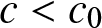 $c \lt c_0$ (left panel), reconnects at the origin at the figure-
 $\infty$ shape for
 $c = c_0$ (middle panel), and splits into two circular bubbles along the real axis for
 $c \gt c_0$ (right panel), where
 $c_0 \approx 1.09213793$ is found from the root of
 $\mathcal{H}'(c)$. The dashed lines show the approximations obtained from the normal form (6.16).

The same as Figure 13 but for the second instance of the figure- $\infty$ bifurcation, which happens when
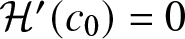 $\mathcal{H}'(c_0) = 0$ for
 $c_0 \approx 1.09228678$.

7. New figure-
$8$ bands arising from the origin

The corresponding bifurcation is seen in panels (m)–(o) of Figure 1. For simplicity, we call it the figure- $8$ bifurcation. Before the bifurcation [panel (m)], there are no circular bands around the origin. Past the bifurcation [panels (n) and (o)], new figure-
 $8$ bands appear from the origin and grow in size.
Section 7.1 develops the criterion for this bifurcation. Section 7.2 gives the derivation of the normal form, which explains how the bifurcation is unfolded. Section 7.3 describes numerical approximations of the coefficients of the normal form, from which we are able to reproduce the bifurcation pattern seen in panels (m)–(o) of Figure 1.
7.1. Criterion of the bifurcation
This bifurcation is due to the double zero eigenvalue of the linear operator
 \begin{equation*}
\mathcal{L} : H^1_{\rm per} \subset L^2_{\rm per} \to L^2_{\rm per},
\end{equation*}
for which Assumption 1 is no longer considered to be true. This corresponds to the fold bifurcation in the existence of the travelling waves with the profile  $\eta \in C^{\infty}_{\rm per}$. The dependence of wave speed
 $c$ versus wave steepness
 $s$ has an extremum (either maximum or minimum). We replace Assumption 1 with the opposite non-generic assumption for the fold bifurcation.
Assumption 5. For the given value of  $c \in (1,c_*)$, there exists an eigenfunction
 $v_0 \in H^1_{\rm per}$ (defined up to scalar multiplication), such that
 $\mathcal{L} v_0 = 0$,
 $v_0$ is even in
 $u$, and
 $\langle 1, v_0 \rangle \neq 0$.
Due to Assumption 5, we have  ${\rm Ker}(\mathcal{L}) = {\rm span}(\eta',v_0)$ so that the decompositions (4.1) and (4.2) are no longer true. Assumption 5 implies that the spectral problem (2.12) for
 $\lambda = 0$ admits a three-dimensional kernel spanned as
 \begin{equation}
\left( \begin{array}{c} \hat{v}_0 \\ \hat{w}_0 \end{array} \right) = a_1 \left( \begin{array}{c} \eta' \\ 0 \end{array} \right) +
a_2 \left( \begin{array}{c} v_0 \\ 0 \end{array} \right) + a_3 \left( \begin{array}{c} 0 \\ 1 \end{array} \right).
\end{equation}
where  $(a_1,a_2,a_3) \in \mathbb{R}^3$.
To construct the generalized eigenfunctions and to determine the algebraic multiplicity of the eigenvalue  $\lambda = 0$ in the spectral problem (2.12), we use the following lemma.
Lemma 7. Let Assumption 5 be true. Then, we have
 \begin{equation*}
\langle \eta, v_0 \rangle \neq 0 \quad \mbox{and} \quad
\langle \mathcal{K} \eta, v_0 \rangle \neq 0.
\end{equation*}
Proof. We rewrite  $\mathcal{L} v_0 = 0$ for
 $v_0 \in H^1_{\rm per}$ as
 \begin{equation}
c^2 \mathcal{K} v_0 - v_0 = (\mathcal{K} \eta) v_0 + \eta \mathcal{K} v_0 + \mathcal{K} (\eta v_0).
\end{equation}
Taking the mean value of (7.2) gives the constraint
 \begin{equation}
\langle 1 + 2 \mathcal{K} \eta, v_0 \rangle = 0.
\end{equation}
Since  $\langle 1, v_0 \rangle \neq 0$ by Assumption 5, we have
 $2 \langle \mathcal{K} \eta, v_0 \rangle = -\langle 1, v_0 \rangle \neq 0$. Taking the inner product of (7.2) with
 $\eta$ and using (1.11) gives another constraint
 \begin{equation}
\langle c^2 \mathcal{K} \eta - \eta, v_0 \rangle = 0.
\end{equation}
Since  $\langle \mathcal{K} \eta, v_0 \rangle \neq 0$, we have
 $\langle \eta, v_0 \rangle = c^2 \langle \mathcal{K} \eta, v_0 \rangle \neq 0$.
Remark 15. Constraints (7.3) and (7.4) in Lemma 7 also follow from identities (2.1) and (2.2) and the self-adjointness of  $\mathcal{L}$ in
 $L^2_{\rm per}$.
Due to the constraints in Lemma 7, there exists only one linearly independent eigenfunction satisfying the linear inhomogeneous system (4.3). It corresponds to  $a_1 = a_2 = 0$, with the explicit solution replacing (4.2) with
 \begin{equation}
\left( \begin{array}{c} \hat{v}_g \\ \hat{w}_g \end{array} \right) = a_3 \left[ \left( \begin{array}{c} -1 \\ 0 \end{array} \right)
\pm i \left( \begin{array}{c} \eta' \\ -c \end{array} \right) \right].
\end{equation}
Therefore, the generalized kernel of the spectral problem (2.12) is exactly four-dimensional under Assumption 5. This implies particularly that the fold bifurcation does not imply the zero-eigenvalue bifurcation in the spectral problem (1.19) for co-periodic perturbations, compared to the bifurcation defined by Assumption 4, see Remark 20.
We now formulate and prove the criterion for the corresponding bifurcation.
Theorem 6 Let Assumption 5 be true. There exist two spectral bands of the modulational stability problem (1.27) crossing  $\lambda = 0$ according to the roots of the characteristic equation given by
 \begin{equation}
\left( \lambda - \frac{i \mu c}{2} \right)^2 = |\mu|^3 \left[ \mathcal{N}(c) - \frac{5c}{4} \mathcal{P}(c) \right] + \mathcal{O}(|\mu|^{7/2}),
\end{equation}
where  $\mathcal{P}(c)$ and
 $\mathcal{N}(c)$ are defined by (2.5) and (2.7) and
 $\mathcal{N}(c) - \frac{5c}{4} \mathcal{P}(c) \neq 0$ is assumed. In addition, similar to Theorems 1 and 5, there exist two other spectral bands, which are subsets of
 $i \mathbb{R}$ and non-degenerate.
Proof. We revisit the proof of Theorem 1, when Assumption 5 replaces Assumption 1. Substituting (7.1) into (1.27) yields the residual terms
 \begin{equation*}
\left\{\begin{array}{l}
i \mu \mathcal{H}_{\pm} \hat{w}_0 + \lambda \mathcal{M}_{\pm} \hat{v}_0, \\
i \mu \mathcal{L}_{\pm} \hat{v}_0 + \lambda (\mathcal{M}_{\pm}^* \hat{w}_0 - 2 c \mathcal{H}_{\pm} \hat{v}_0).
\end{array} \right.
\end{equation*}
Projecting the first equation to  ${\rm Ker}(\mathcal{K}) = {\rm span}(1)$ in the first equation and the second equation to
 ${\rm Ker}(\mathcal{L}) = {\rm span}(\eta',v_0)$ yields
 \begin{equation}
\left\{\begin{array}{l}
i \mu \langle 1, \mathcal{H}_{\pm} \hat{w}_0 \rangle + \lambda \langle 1, \mathcal{M}_{\pm} \hat{v}_0 \rangle, \\
i\mu \langle \eta', \mathcal{L}_{\pm} \hat{v}_0 \rangle
+ \lambda \langle \eta', (\mathcal{M}_{\pm}^* \hat{w}_0 - 2 c \mathcal{H}_{\pm} \hat{v}_0) \rangle, \\
i\mu \langle v_0, \mathcal{L}_{\pm} \hat{v}_0 \rangle
+ \lambda \langle v_0, (\mathcal{M}_{\pm}^* \hat{w}_0 - 2 c \mathcal{H}_{\pm} \hat{v}_0) \rangle.
\end{array} \right.
\end{equation}
We substitute (7.1) into (7.7) and obtain
 \begin{equation}
\left( \begin{matrix}
0 & 0 & \mp \mu \\
0 & i \mu \langle \eta, v_0 \rangle - 2 c \lambda \langle \mathcal{K} \eta, v_0 \rangle & 0 \\
- i \mu \langle \eta, v_0 \rangle + 2 c \lambda \langle \mathcal{K} \eta, v_0 \rangle &
\mp (2 i c \lambda + c^2 \mu) |\langle 1, v_0 \rangle |^2 \pm 2 \mu \langle \eta, v_0 \rangle \langle 1, v_0 \rangle & 0
\end{matrix} \right) \left( \begin{matrix} a_1 \\ a_2 \\ a_3 \end{matrix} \right),
\end{equation}
where we have used (1.21), (1.23), (1.26), (2.3),  $\mathcal{L}_{\pm}^* = -\mathcal{L}_{\pm}$ and
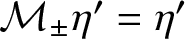 $\mathcal{M}_{\pm} \eta' = \eta'$, and
 $\langle v_0, \mathcal{M}^* 1 \rangle = \langle v_0, 1 + 2 \mathcal{K} \eta \rangle = 0$ due to (7.3).
Similarly to the system (4.6) in the proof of Theorem 1, the system (7.8) suggests two different scalings for the characteristic equations, one is related to  $(a_1,a_2) = 0$,
 $a_3 \neq 0$ and the other one is related to
 $(a_1,a_2) \neq (0,0)$ and
 $a_3 = 0$. The subspace
 $(a_1,a_2) = 0$,
 $a_3 \neq 0$ is analysed in exactly the same way as in the proof of Theorem 1 and it yields two spectral bands with the scaling
 $\lambda = \mathcal{O}(\mu^{1/2})$, which are subsets of
 $i \mathbb{R}$ and non-degenerate. On the other hand, the subspace
 $(a_1,a_2) \neq (0,0)$ and
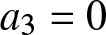 $a_3 = 0$ yields two spectral bands, which are degenerate at the leading order. It follows from (7.8) that the two degenerate spectral bands are given by the leading-order approximation
 \begin{equation}
\lambda \approx \frac{i \mu \langle \eta, v_0 \rangle}{2c \langle \mathcal{K} \eta, v_0 \rangle} = \frac{i c \mu}{2},
\end{equation}
where we have used (7.4). If  $\mu \neq 0$, the third equation in (7.8) determines uniquely
 $a_2$ and the first equation in (7.8) determines uniquely
 $a_3$ since
 $\pm 2 \mu \langle \eta, v_0 \rangle \langle 1, v_0 \rangle \neq 0$. Hence, the characteristic equation for the two degenerate spectral bands is obtained from the second equation, where we can set
 $a_1 = 1$ without loss of generality. Based on the justification analysis in Section 3.4, leading to the eigenvalue splitting formulas (3.25) and (3.27), we introduce the asymptotic expansions:
 \begin{equation}
\mu = \epsilon \mu_1, \quad \lambda = \epsilon \lambda_1 + \epsilon^{3/2} \lambda_{3/2} + \mathcal{O}(\epsilon^2)
\end{equation}
and
 \begin{equation}
\left( \begin{array}{c} \hat{v} \\ \hat{w} \end{array} \right) = \left( \begin{array}{c} \eta' \\ 0 \end{array} \right) + \epsilon^{1/2} a \left( \begin{array}{c} v_0 \\ 0 \end{array} \right) + \epsilon \left( \begin{array}{c} \hat{v}_1 \\ \hat{w}_1 \end{array} \right) + \epsilon^{3/2} \left( \begin{array}{c} \hat{v}_{3/2} \\ \hat{w}_{3/2} \end{array} \right) + \epsilon^2 \left( \begin{array}{c} \hat{v}_2 \\ \hat{w}_2 \end{array} \right) + \mathcal{O}(\epsilon^{5/2}),
\end{equation}
where  $\epsilon \gt 0$ is a small parameter,
 $\mu_1 \neq 0$ is fixed,
 $a \in \mathbb{R}$ is arbitrary at the leading order and the correction terms up to the order of
 $\mathcal{O}(\epsilon^2)$ are to be computed recursively in function space
 $H^1_{\rm per} \times H^1_{\rm per}$.
 $\underline{\boldsymbol{\mathrm{Order}} \ \mathcal{O}(\epsilon)}$: We get the linear inhomogeneous system
 \begin{equation}
\left\{\begin{array}{ll}
\mathcal{K} \hat{w}_1 &= \lambda_1 \mathcal{M} \eta', \\
\mathcal{L} \hat{v}_1 &= - 2 c \lambda_1 \mathcal{H} \eta' + i \mu_1 \mathcal{L}_{\pm} \eta'.
\end{array}
\right.
\end{equation}
Since  $\mathcal{M} \eta' = \eta'$,
 $-\mathcal{H} \eta' = \mathcal{K} \eta$ and
 $\mathcal{L}_{\pm} \eta' = -\eta$, Fredholm conditions are satisfied for this system if and only if
 \begin{equation}
\lambda_1 = \frac{i c \mu_1}{2},
\end{equation}
in agreement with (7.9). There exists a periodic solution of the system (7.12) in the form
 \begin{equation}
\left( \begin{array}{c} \hat{v}_1 \\ \hat{w}_1 \end{array} \right) = \left( \begin{array}{c} -i \mu_1 \eta \\ \lambda_1 \mathcal{H} \eta \end{array} \right) + a_1 \left( \begin{array}{c} v_0 \\ 0 \end{array} \right) + b_1 \left( \begin{array}{c} 0 \\ 1 \end{array} \right),
\end{equation}
where we have introduced projections to the second and third elements of the kernel (7.1) with coordinates 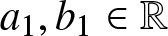 $a_1, b_1 \in \mathbb{R}$ and a solution
 $\eta = -\mathcal{L}^{-1} (c^2 \mathcal{K} \eta - \eta) \in H^1_{\rm per}$ from (2.2).
 $\underline{\boldsymbol{\mathrm{Order}} \ \mathcal{O}(\epsilon^{3/2})}$: We get the linear inhomogeneous system
 \begin{equation}
\left\{\begin{array}{ll}
\mathcal{K} \hat{w}_{3/2} &= \lambda_1 a \mathcal{M}_{\pm} v_0 + \lambda_{3/2} \mathcal{M} \eta', \\
\mathcal{L} \hat{v}_{3/2} &= - 2 c \lambda_1 a \mathcal{H}_{\pm} v_0 + i \mu_1 a \mathcal{L}_{\pm} v_0 - 2 c \lambda_{3/2} \mathcal{H} \eta'.
\end{array}
\right.
\end{equation}
Since  $\mathcal{M}_{\pm} v_0, \mathcal{M} \eta' \perp {\rm Ker}(\mathcal{K})$ due to the constraint (7.3), there exists always a solution
 $\hat{w}_{3/2} \in H^1_{\rm per}$ to the first equation of the system (7.15). Projection of the right-hand side of the second equation of the system (7.15) to
 $\eta'$ yields
 \begin{equation*}
\langle \eta', - 2 c \lambda_1 a \mathcal{H}_{\pm} v_0 + i \mu_1 a \mathcal{L}_{\pm} v_0 - 2 c \lambda_{3/2} \mathcal{H} \eta'\rangle
= -2c \lambda_1 a \langle \mathcal{K} \eta, v_0 \rangle + i \mu_1 a \langle \eta, v_0 \rangle = 0,
\end{equation*}
where the last equality is due to the constraint (7.4) and the definition of  $\lambda_1$ in (7.13). Finally, projection of the right-hand side of the second equation of the system (7.15) to
 $v_0$ yields
 \begin{align*}
& \quad
\langle v_0, - 2 c \lambda_1 a \mathcal{H}_{\pm} v_0 + i \mu_1 a \mathcal{L}_{\pm} v_0 - 2 c \lambda_{3/2} \mathcal{H} \eta'\rangle \\
&= \mp 2 i c \lambda_1 a |\langle 1, v_0 \rangle |^2 \mp \mu_1 a \left[ c^2 |\langle 1, v_0 \rangle |^2 - 2 \langle \eta, v_0 \rangle \langle 1, v_0 \rangle \right] + 2 c \lambda_{3/2} \langle \mathcal{K} \eta, v_0 \rangle = 0.
\end{align*}
In view of (7.13), we obtain a unique expression for the coefficient  $a$ given by
 \begin{equation}
a = \mp \frac{c \lambda_{3/2} \langle \mathcal{K} \eta, v_0 \rangle}{\mu_1 \langle \eta, v_0 \rangle \langle 1, v_0 \rangle } = \mp \frac{\lambda_{3/2}}{c \mu_1 \langle 1, v_0 \rangle },
\end{equation}
where we have used (7.4) again. Since the three constraints are satisfied, there exists a periodic solution of the system (7.15) in the form
 \begin{equation}
\left( \begin{array}{c} \hat{v}_{3/2} \\ \hat{w}_{3/2} \end{array} \right) = \lambda_{3/2} \left( \begin{array}{c} \tilde{v}_{3/2} \\ \tilde{w}_{3/2} \end{array} \right) + a_{3/2} \left( \begin{array}{c} v_0 \\ 0 \end{array} \right) + b_{3/2} \left( \begin{array}{c} 0 \\ 1 \end{array} \right),
\end{equation}
where  $(\tilde{v}_{3/2},\tilde{w}_{3/2})$ are uniquely defined from (7.15) with
 $a$ being defined by (7.16), whereas
 $a_{3/2}, b_{3/2} \in \mathbb{R}$ are renormalizations of the projections to the second and third element of the kernel (7.1).
 $\underline{\boldsymbol{\mathrm{Order}} \ \mathcal{O}(\epsilon^2)}$: We get the linear inhomogeneous system
 \begin{equation}
\left\{\begin{array}{ll}
\mathcal{K} \hat{w}_2 &= \lambda_1 \mathcal{M}_{\pm} \hat{v}_1 + \lambda_{3/2} a \mathcal{M}_{\pm} v_0 + i \mu_1 \mathcal{H}_{\pm} \hat{w}_1, \\
\mathcal{L} \hat{v}_2 &= \lambda_1 \left( \mathcal{M}_{\pm}^* \hat{w}_1 - 2 c \mathcal{H}_{\pm} \hat{v}_1 \right)
+ i \mu_1 \mathcal{L}_{\pm} \hat{v}_1 - 2 c \lambda_{3/2} a \mathcal{H}_{\pm} v_0.
\end{array}
\right.
\end{equation}
Projection of the right-hand side of the first equation of the system (7.18) to  $1$ yields
 \begin{align*}
\langle 1, \lambda_1\mathcal{M}_{\pm} \hat{v}_1 + \lambda_{3/2} a \mathcal{M}_{\pm} v_0 + i \mu_1 \mathcal{H}_{\pm} \hat{w}_1 \rangle = -i \lambda_1 \mu_1 \langle 1, \mathcal{M}_{\pm} \eta \rangle \mp \mu_1 b_1 = 0.
\end{align*}
This defines the coefficient  $b_1$ uniquely by
 \begin{equation}
b_1 = \mp i \lambda_1 \langle 1 + 2 \mathcal{K} \eta, \eta \rangle
\end{equation}
since  $\mu_1 \neq 0$ is assumed. Projection of the right-hand side of the second equation of the system (7.18) to
 $\eta'$ yields
 \begin{align*}
& \quad
\langle \eta', \lambda_1 \left( \mathcal{M}_{\pm}^* \hat{w}_1 - 2 c \mathcal{H}_{\pm} \hat{v}_1 \right)
+ i \mu_1 \mathcal{L}_{\pm} \hat{v}_1 - 2 c \lambda_{3/2} a \mathcal{H}_{\pm} v_0 \rangle \\
&= \lambda_1^2 \langle \mathcal{K} \eta, \eta \rangle + 2 i c \mu_1 \lambda_1 \langle \mathcal{K} \eta, \eta \rangle + \mu_1^2
\langle \eta, \eta \rangle + a_1 (-2 c \lambda_1 \langle \mathcal{K} \eta, v_0 \rangle + i \mu_1 \langle \eta, v_0 \rangle)
- 2 c a \lambda_{3/2} \langle \mathcal{K} \eta, v_0 \rangle \\
&= - \mu_1^2 \left[ \langle (c^2 \mathcal{K} \eta - \eta, \eta \rangle + \frac{c^2}{4} \langle \mathcal{K} \eta, \eta \rangle \right]
- 2 c a \lambda_{3/2} \langle \mathcal{K} \eta, v_0 \rangle = 0,
\end{align*}
where the last equality is due to the constraint (7.4) and the definition of  $\lambda_1$ in (7.13). Since
 $a$ is defined by (7.16) and the relation (7.3) holds, this yields
 \begin{equation}
\lambda_{3/2}^2 = \pm \mu_1^3 \left[ \mathcal{N}(c) - \frac{5c}{4} \mathcal{P}(c) \right], \quad \pm \mu_1 \gt 0,
\end{equation}
which is equivalent to the characteristic equation (7.6). Finally, projection of the right-hand side of the second equation of the system (7.18) to  $v_0$ yields
 \begin{align*}
& \quad
\langle v_0, \lambda_1 \left( \mathcal{M}_{\pm}^* \hat{w}_1 - 2 c \mathcal{H}_{\pm} \hat{v}_1 \right)
+ i \mu_1 \mathcal{L}_{\pm} \hat{v}_1 - 2 c \lambda_{3/2} a \mathcal{H}_{\pm} v_0 \rangle \\
&= \lambda_1^2 \langle v_0, \mathcal{M}_{\pm}^* \mathcal{H} \eta \rangle + 2 i c \mu_1 \lambda_1 \langle v_0, \mathcal{H}_{\pm} \eta \rangle + \mu_1^2
\langle v_0, \mathcal{L}_{\pm} \eta \rangle \\
& \qquad
\mp 2 i c \lambda_1 a_1 |\langle 1, v_0 \rangle |^2 \mp \mu_1 a_1 \left[ c^2 |\langle 1, v_0 \rangle |^2 - 2 \langle \eta, v_0 \rangle \langle 1, v_0 \rangle \right] \mp 2 i c \lambda_{3/2} a |\langle 1, v_0 \rangle |^2 = 0.
\end{align*}
In view of (7.13), (7.16) and (7.20), this equation yields a unique expression of  $a_1$ in terms of
 $\mu_1$, which we do not write. Since the three constraints are satisfied, there exists a periodic solution of the system (7.18). The asymptotic expansion (7.11) is defined by (7.14) and (7.17). The two roots of the characteristic equation (7.6) are non-degenerate if
 $\mathcal{N}(c) - \frac{5c}{4} \mathcal{P}(c) \neq 0$.
Remark 16. If  $\mathcal{N}(c) - \frac{5c}{4} \mathcal{P}(c) \lt 0$, then the two non-degenerate spectral bands given by roots
 $\lambda^{\pm}(\mu)$ of the characteristic equation (7.6) satisfy
 $\lambda^{\pm}(\mu) \in i \mathbb{R}$ and
 $\lambda^+(\mu) \neq \lambda^-(\mu)$ for
 $\mu \neq 0$. In this case, there exist no figure-
 $8$ bands at the fold bifurcation point.
Remark 17. We can confirm  $\mathcal{N}(c) - \frac{5c}{4} \mathcal{P}(c) \lt 0$ for the small-amplitude expansions (1.13) and (1.14), for which
 \begin{align*}
\mathcal{N}(c) &= \frac{1}{2} a^2 + \mathcal{O}(a^4), \\
\mathcal{P}(c) &= \frac{1}{2} a^2 + \mathcal{O}(a^4),
\end{align*}
which yields
 \begin{align*}
\mathcal{N}(c) - \frac{5c}{4} \mathcal{P}(c) = -\frac{1}{8} a^2 + \mathcal{O}(a^2).
\end{align*}
However, Assumption 5 is not true in the small-amplitude limit because  $\eta'(u) \sim \sin(u)$,
 $v_0(u) \sim \cos(u)$ and
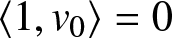 $\langle 1, v_0 \rangle = 0$. New figure-
 $8$ bands bifurcating in the small-amplitude limit are studied in Appendix A, where it is shown that the normal form for the figure-
 $8$ bifurcation in the small-amplitude limit is different from (7.6), see equation (A.1) also derived in [Reference Berti, Maspero and Ventura6, Reference Creedon and Deconinck14].
7.2. Normal form of the bifurcation
In order to obtain the figure- $8$ bands as a result of the bifurcation of Theorem 6, we need to understand how the bifurcation in the family of travelling waves is unfolded for
 $c \neq c_0$. The following lemma gives the bifurcation result based on the standard method of Lyapunov–Schmidt reductions.
Lemma 8. Let  $c_0 \in (1,c_*)$ be the bifurcation point, under which Assumption 5 holds with the profile
 $\eta_0 \in C^{\infty}_{\rm per}$. If
 $\langle \mathcal{K} v_0, v_0^2 \rangle \neq 0$, then there exist two solutions of Babenko’s equation (1.11) for
 $c \neq c_0$ close to
 $c_0$ with
 \begin{equation}
{\rm sgn}(c-c_0) = {\rm sgn}\left( \langle \mathcal{K} v_0, v_0^2 \rangle \langle \mathcal{K} \eta_0, v_0 \rangle \right)
\end{equation}
such that their profiles satisfy
 \begin{equation}
\| \eta - \eta_0 \|_{H^1_{\rm per}} \leq C \sqrt{|c-c_0|},
\end{equation}
for a positive constant  $C$ in a small neighbourhood of
 $c = c_0$.
Proof. Let  $c^2 = c_0^2 + \delta \varepsilon^2$, where
 $\delta \in \mathbb{R}$ is to be determined and
 $\varepsilon \in \mathbb{R}$ is a small parameter unrelated to
 $\epsilon$. By using the Lyapunov–Schmidt decomposition, we represent an even solution
 $\eta \in C^{\infty}_{\rm per}$ of Babenko’s equation (1.11) in the form:
 \begin{equation}
\eta = \eta_0 + \varepsilon v_0 + \varepsilon^2 \mathfrak{v}, \quad \langle v_0, \mathfrak{v} \rangle = 0,
\end{equation}
where  $\mathfrak{v} \in H^1_{\rm per,e} = \{f \in H^1_{\rm per} : \; f(-x) = f(x), \quad x \in \mathbb{T} \}$. Babenko’s equation (1.11) is rewritten in the perturbed form
 \begin{equation}
\mathcal{L}_0 \mathfrak{v} + \delta \mathcal{K} (\eta_0 + \varepsilon v_0 + \varepsilon^2 \mathfrak{v}) = \frac{1}{2} \mathcal{K} (v_0 + \varepsilon \mathfrak{v})^2 + (v_0 + \varepsilon \mathfrak{v}) \mathcal{K} (v_0 + \varepsilon \mathfrak{v}),
\end{equation}
where  $\mathcal{L}_0$ is the linearized Babenko’s operator for
 $c = c_0$ and
 $\eta = \eta_0$. Since
 ${\rm Ker}(\mathcal{L}_0) = {\rm span}(v_0)$ in
 $H^1_{\rm per,e}$, we define
 $\delta$ from the bifurcation equation after projecting (7.24) to
 $v_0$:
 \begin{equation}
\delta \langle \mathcal{K} (\eta_0 + \varepsilon v_0 + \varepsilon^2 \mathfrak{v}), v_0 \rangle = \frac{1}{2}
\langle \mathcal{K} (v_0 + \varepsilon \mathfrak{v})^2, v_0 \rangle + \langle \mathcal{K} (v_0 + \varepsilon \mathfrak{v}), v_0 (v_0 + \varepsilon \mathfrak{v}) \rangle.
\end{equation}
By the implicit function theorem in  $H^1_{\rm per,e} |_{\{v_0 \}^{\perp}}$, there exists a unique solution of (7.24) under the constraint (7.25) for every small
 $\varepsilon \in \mathbb{R}$ such that
 $\mathfrak{v} \in H^1_{\rm per,e} |_{\{v_0 \}^{\perp}}$ and
 \begin{equation*}
\| \mathfrak{v} \|_{H^1_{\rm per}} \leq C \varepsilon^2
\end{equation*}
for some  $C \gt 0$ in a small neighbourhood of
 $\varepsilon = 0$. Substituting this solution into (7.25), we obtain
 \begin{equation}
\delta = \delta_0 + \mathcal{O}(\varepsilon), \qquad \delta_0 = \frac{3}{2} \frac{\langle \mathcal{K} v_0, v_0^2 \rangle}{\langle \mathcal{K} \eta_0, v_0 \rangle}.
\end{equation}
Since  $\langle \mathcal{K} \eta_0, v_0 \rangle \neq 0$ by Assumption 5 and
 $\langle \mathcal{K} v_0, v_0^2 \rangle \neq 0$ by the assumption of the lemma, we have
 $\delta_0 \neq 0$, which implies that
 $\delta \neq 0$ for every small
 $\varepsilon$. The bound (7.22) follows from the decomposition (7.23) and the bound on
 $\mathfrak{v} \in H^1_{\rm per,e} |_{\{v_0 \}^{\perp}}$. Two possible solutions for
 $\varepsilon \neq 0$ exist for
 ${\rm sgn}(c-c_0) = {\rm sgn}(\delta_0)$, which justifies the condition (7.21).
Remark 18. The bifurcation in Lemma 8 is referred to as the fold bifurcation. No solutions of Babenko’s equation (1.11) for  $c \neq c_0$ close to
 $c_0$ exist in a local neighbourhood of
 $\eta_0 \in C^{\infty}_{\rm per}$ if the sign of
 $(c-c_0)$ is opposite to (7.21).
Remark 19. Expanding  $\mathcal{L}$ at the profile
 $\eta$ in Lemma 8 near
 $\varepsilon = 0$ yields
 \begin{equation}
\mathcal{L} = \mathcal{L}_0 + \varepsilon \mathcal{L}_1 + \mathcal{O}(\varepsilon^2),
\end{equation}
where
 \begin{align*}
\mathcal{L}_0 &= c_0^2 \mathcal{K} - 1 - \mathcal{K} \eta_0 - \eta_0 \mathcal{K} - \mathcal{K}(\eta_0 \cdot), \\
\mathcal{L}_1 &= -(\mathcal{K} v_0) - v_0 \mathcal{K} - \mathcal{K}(v_0 \cdot).
\end{align*}
The perturbation theory for the small eigenvalue  $\lambda(\varepsilon)$ of
 $\mathcal{L}$ bifurcating from
 $\lambda(0) = 0$ at
 $\varepsilon = 0$ yields
 \begin{equation*}
\lambda(\varepsilon) = -3 \varepsilon \frac{\langle \mathcal{K} v_0, v_0^2 \rangle}{\| v_0 \|^2_{L^2}} + \mathcal{O}(\varepsilon^2).
\end{equation*}
Since  $\langle \mathcal{K} v_0, v_0^2 \rangle \neq 0$ and there are two roots of
 $\varepsilon$ with opposite signs for every
 $c \neq c_0$ near
 $c = c_0$ satisfying (7.21), it is clear that one root corresponds to the small positive eigenvalue
 $\lambda(\varepsilon) \gt 0$ and the other root corresponds to the small negative eigenvalue
 $\lambda(\varepsilon) \lt 0$.
Remark 20. Although  $\mathcal{L}$ admits a new small eigenvalue for small
 $\varepsilon$, see Remark 19, no new small eigenvalues near
 $\lambda = 0$ bifurcate in the spectral stability problem (1.19) for small
 $\varepsilon$. This is because
 $\langle \eta', \mathcal{H} v_0 \rangle = \langle \mathcal{K} \eta, v_0 \rangle \neq 0$ due to Assumption 5 and Lemma 7. The Fredholm condition for the generalized kernel is not satisfied for the subspace
 $(a_1,a_2)$ in (7.1) and no generalized eigenvectors exist in this subspace. There is exactly one generalized eigenvector associated with the subspace
 $a_3$ as in (7.5). In other words, the quadruple algebraic multiplicity of
 $\lambda = 0$ in the spectral problem (1.19) persists both for
 $c = c_0$ and
 $c \neq c_0$. The only difference between the two cases is the geometric multiplicity of
 $\lambda = 0$ in the spectral problem (1.19): it is equal to three for
 $c = c_0$ and to two for
 $c \neq c_0$.
Finally, we combine the results of Theorem 6 and Lemma 8 to get the normal form for the figure- $8$ bifurcation.
Theorem 7 Let  $c = c_0$ be the fold bifurcation point of Lemma 8, where Assumption 5 holds. The characteristic equation for the two spectral bands crossing
 $\lambda = 0$ as in Theorem 6 is given by
 \begin{equation}
\left( \lambda - \frac{i \mu c_0}{2} \right)^2 = \mu^2 \left[ \mathcal{N}(c_0) - \frac{5c_0}{4} \mathcal{P}(c_0) \right]
\left[ |\mu| + \frac{\delta_0 \varepsilon}{c_0^2 \langle 1, v_0 \rangle} \right] + \mathcal{O}(|\mu|^{7/2}),
\end{equation}
where  $c^2 = c_0^2 + \delta_0 \varepsilon^2 + \mathcal{O}(\varepsilon^3)$ with
 $\delta_0$ given by (7.26) and with
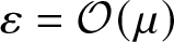 $\varepsilon = \mathcal{O}(\mu)$ at the leading-order balance.
Proof. We use (7.10) and (7.11) for  $(\mu,\lambda) \in \mathbb{R} \times \mathbb{C}$ near
 $(0,0)$, and
 $(\hat{v},\hat{w}) \in H^1_{\rm per} \times H^1_{\rm per}$. Since the profile
 $\eta$ is also expanded for
 $c \neq c_0$, we use (7.23) with
 $\varepsilon = \sigma \epsilon$, where
 $\epsilon \gt 0$ and
 $\sigma = \pm 1$ incorporate the different signs of
 $\varepsilon$ at the two branches. By Lemma 8, we also have
 $c^2 = c_0^2 + \delta \epsilon^2$ with
 $\delta = \delta_0 + \mathcal{O}(\varepsilon)$ given by (7.26). Due to the perturbation expansion (7.23), we should use the expansion (7.27) for
 $\mathcal{L}$ and similar expansions for
 $\mathcal{M}_{\pm}$,
 $\mathcal{M}^*_{\pm}$ and
 $\mathcal{L}_{\pm}$ (which do not affect the outcomes of computations).
 $\underline{\boldsymbol{\mathrm{Order}} \ \mathcal{O}(\epsilon)}$: We get the following modification of the linear inhomogeneous system (7.12):
 \begin{equation}
\left\{\begin{array}{ll}
\mathcal{K} \hat{w}_1 &= \lambda_1 \mathcal{M} \eta'_0, \\
\mathcal{L}_0 \hat{v}_1 + \sigma \mathcal{L}_1 \eta'_0 &= - 2 c_0 \lambda_1 \mathcal{H} \eta'_0 + i \mu_1 \mathcal{L}_{\pm} \eta'_0,
\end{array}
\right.
\end{equation}
where  $\sigma = \pm 1$ is due to
 $\varepsilon = \pm \epsilon$. Since
 \begin{equation*}
\mathcal{L}_0 v_0' + \mathcal{L}_1 \eta_0' = 0
\end{equation*}
follows from the first order in  $\mathcal{O}(\varepsilon)$ of
 $\mathcal{L} \eta' = 0$, the solution to the system (7.29) is modified compared to (7.14) as follows:
 \begin{align*}
\left( \begin{array}{c} \hat{v}_1 \\ \hat{w}_1 \end{array} \right) = \left( \begin{array}{c} -i \mu_1 \eta_0 \\ \lambda_1 \mathcal{H} \eta_0 \end{array} \right) + a_1 \left( \begin{array}{c} v_0 \\ 0 \end{array} \right) + b_1 \left( \begin{array}{c} 0 \\ 1 \end{array} \right) + \sigma
\left( \begin{array}{c} v_0' \\ 0 \end{array} \right).
\end{align*}
In addition, we recall that 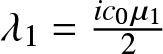 $\lambda_1 = \frac{i c_0 \mu_1}{2}$ from (7.13).
 $\underline{\boldsymbol{\mathrm{Order}} \ \mathcal{O}(\epsilon^{3/2})}$: We get the following modification of the linear inhomogeneous system (7.15):
 \begin{equation}
\left\{\begin{array}{ll}
\mathcal{K} \hat{w}_{3/2} &= \lambda_1 a \mathcal{M}_{\pm} v_0 + \lambda_{3/2} \mathcal{M} \eta'_0, \\
\mathcal{L} \hat{v}_{3/2} + a \sigma \mathcal{L}_1 v_0 &= - 2 c_0 \lambda_1 a \mathcal{H}_{\pm} v_0 + i \mu_1 a \mathcal{L}_{\pm} v_0 - 2 c_0 \lambda_{3/2} \mathcal{H} \eta'_0.
\end{array}
\right.
\end{equation}
The first equation of the system (7.30) is the same as in (7.15) with the same solution. Since  $\mathcal{L}_1 v_0$ is even, there is no contribution from the new term of the second equation of the system (7.15) to the orthogonality condition with respect to
 $\eta'$. However, we get a modification of the orthogonality condition with respect to
 $v_0$ as follows:
 \begin{align*}
& \quad
\langle v_0, - 2 c_0 \lambda_1 a \mathcal{H}_{\pm} v_0 + i \mu_1 a \mathcal{L}_{\pm} v_0 - 2 c_0 \lambda_{3/2} \mathcal{H} \eta_0' - a \sigma \mathcal{L}_1 v_0 \rangle \\
&= \mp 2 i c_0 \lambda_1 a |\langle 1, v_0 \rangle |^2 \mp \mu_1 a \left[ c_0^2 |\langle 1, v_0 \rangle |^2 - 2 \langle \eta_0, v_0 \rangle \langle 1, v_0 \rangle \right] + 2 c_0 \lambda_{3/2} \langle \mathcal{K} \eta_0, v_0 \rangle + 3 a \sigma \langle \mathcal{K} v_0, v_0^2 \rangle
= 0.
\end{align*}
Similarly to (7.16), we use 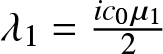 $\lambda_1 = \frac{i c_0 \mu_1}{2}$ and obtain a unique expression for the coefficient
 $a$ given by
 \begin{equation}
a = -\frac{c_0 \lambda_{3/2} \langle \mathcal{K} \eta_0, v_0 \rangle}{|\mu_1| \langle \eta_0, v_0 \rangle \langle 1, v_0 \rangle + \frac{3}{2} \sigma \langle \mathcal{K} v_0, v_0^2 \rangle}
= -\frac{\lambda_{3/2}}{c_0 |\mu_1| \langle 1, v_0 \rangle + \sigma \delta_0},
\end{equation}
where we have used (7.26). Since the three constraints are satisfied, there exists a periodic solution of the system (7.30), which does not affect computations at the next order.
 $\underline{\boldsymbol{\mathrm{Order}} \ \mathcal{O}(\epsilon^2)}$: We get the following modification of the linear inhomogeneous system (7.18):
 \begin{equation*}
\left\{\begin{array}{ll}
\mathcal{K} \hat{w}_2 &= \lambda_1 \mathcal{M}_{\pm} \hat{v}_1 + \lambda_{3/2} a \mathcal{M}_{\pm} v_0 + i \mu_1 \mathcal{H}_{\pm} \hat{w}_1 + \lambda_1 \sigma \mathcal{M}_{\pm}^{(1)} \eta_0', \\
\mathcal{L} \hat{v}_2 + \mathcal{L}_1 \hat{v}_1 + \mathcal{L}_2 \eta_0' &= \lambda_1 \left( \mathcal{M}_{\pm}^* \hat{w}_1 - 2 c_0 \mathcal{H}_{\pm} \hat{v}_1 \right)
+ i \mu_1 \mathcal{L}_{\pm} \hat{v}_1 - 2 c_0 \lambda_{3/2} a \mathcal{H}_{\pm} v_0 + i \mu_1 \sigma \mathcal{L}_{\pm}^{(1)} \eta_0',
\end{array}
\right.
\end{equation*}
where  $\mathcal{L}_{\pm}^{(1)}$ and
 $\mathcal{M}_{\pm}^{(1)}$ appear in the expansion of
 $\mathcal{L}_{\pm}$ and
 $\mathcal{M}_{\pm}$ at the first order of
 $\mathcal{O}(\varepsilon)$. Since
 $\mathcal{M}_{\pm}^{(1)} \eta_0'$ is odd, it does not contribute to the solvability condition for the first equation of the system so that the coefficient
 $b_1$ is still uniquely defined by the expression (7.19).
The second equation of the system is solved under two orthogonality conditions with respect to  $\eta_0'$ and
 $v_0$. Recall that the orthogonality condition to
 $v_0$ defines uniquely the parameter
 $a_1$; hence, it will not be written. Finally, the orthogonality condition to
 $\eta_0'$ is not affected by the term
 $\mathcal{L}_{\pm}^{(1)} \eta_0'$ since it is even, whereas
 $\eta_0'$ is odd. Similarly, it follows from the second order in
 $\mathcal{O}(\varepsilon^2)$ of
 $\mathcal{L} \eta' = 0$ that
 \begin{equation*}
\mathcal{L}_0 \mathfrak{v}_0' + \mathcal{L}_1 v_0' + \mathcal{L}_2 \eta_0' = 0,
\end{equation*}
where  $\mathfrak{v}_0$ is the leading order in the expansion (7.23). This implies that the odd part of
 $\mathcal{L}_1 \hat{v}_1 + \mathcal{L}_2 \eta_0'$ does not contribute to the orthogonality to
 $\eta_0'$. The even part of
 $\mathcal{L}_1 \hat{v}_1 + \mathcal{L}_2 \eta_0'$ does not contribute either, due to the different parity from the parity of
 $\eta_0'$. As a result, we obtain the same orthogonality condition as in the proof of Theorem 6:
 \begin{align*}
- \mu_1^2 \left[ \frac{5 c_0}{4} \mathcal{P}(c_0) - \mathcal{N}(c_0) \right]
- 2 c_0 a \lambda_{3/2} \langle \mathcal{K} \eta_0, v_0 \rangle = 0.
\end{align*}
Substituting (7.31) yields
 \begin{equation*}
\lambda_{3/2}^2 = \mu_1^2 \left[ \mathcal{N}(c_0) - \frac{5c_0}{4} \mathcal{P}(c_0) \right] \left[ |\mu_1| + \frac{\sigma \delta_0}{c_0 \langle 1, v_0 \rangle}
\right],
\end{equation*}
which is equivalent to the characteristic equation (7.6) due to the expansion (7.10) and  $c^2 = c_0^2 + \varepsilon^2 \delta_0 + \mathcal{O}(\varepsilon^3)$ with
 $\varepsilon = \sigma \epsilon$.
Remark 21. New figure- $8$ bands appear past the bifurcation point
 $c = c_0$ if
 \begin{equation*}
\mathcal{N}(c_0) - \frac{5c_0}{4} \mathcal{P}(c_0) \lt 0
\end{equation*}
see Remark 16. If  $c = c_0$, both spectral bands in the characteristic equation (7.28) satisfy
 $\lambda^{\pm}(\mu) \in i \mathbb{R}$ and
 $\lambda^+(\mu) \neq \lambda^-(\mu)$ for
 $\mu \neq 0$. Since the sign of
 $\varepsilon$ in Lemma 8 is opposite between the two branches near the fold bifurcation, one branch for
 $c \neq c_0$ still has
 $\lambda^{\pm}(\mu) \in i \mathbb{R}$ and
 $\lambda^+(\mu) \neq \lambda^-(\mu)$ for
 $\mu \neq 0$, whereas the other branch has the new figure-
 $8$ bands with the maximum corresponding to
 \begin{equation*}
\mu = \frac{|\delta_0 \varepsilon|}{c_0^2 |\langle 1, v_0 \rangle|} +
\mathcal{O}(|\varepsilon|^{3/2}).
\end{equation*}
7.3. Numerical results
The criterion for the bifurcation is a double zero eigenvalue of  $\mathcal{L}$ in
 $L^2_{\rm per}$, which coincides with the extremal point of the speed
 $c$ versus steepness
 $s$ shown in the vertical line of Figure 2. We compute eigenvalues of
 $\mathcal{L}$ in
 $L^2_{\rm per}$ and show them in Figure 3 by green lines. At the green circles, there exists an even eigenfunction
 $v_0 \in H^1_{\rm per}$ in addition to the odd eigenfunction
 $\eta' \in H^1_{\rm per}$. The numerical solution of the eigenvalue problem is obtained via the shift-and-invert method, see [Reference Dyachenko and Semenova24]. Once
 $v_0$ has been determined, we compute the parameter
 $\varepsilon$ and the average value
 $\langle 1, v_0\rangle$ to verify that it is nonzero according to the Assumption 5.
The corresponding steepness  $s_0$ and speed
 $c_0$ for the figure-8 bifurcation are recorded in Table 5, where we also show the coefficients
 $\langle 1, v_0 \rangle$,
 $\delta_0$ and
 $\mathcal{N}(c_0) - \frac{5 c_0}{4} \mathcal{P}(c_0)$ of the normal form (7.28). We note that
 $\langle 1, v_0\rangle \neq 0$ and
 $\mathcal{N}(c_0) - \frac{5 c_0}{4} \mathcal{P}(c_0) \lt 0$, so that the new figure-8 appears past the fold bifurcation, according to Remark 21.
Parameters of the first nontrivial figure- $8$ bifurcation

Table 5 Long description
Five parameters are listed for a single case: s 0, c 0, the inner product of 1 with v 0, delta 0, and the expression labeled, calligraphic N of c 0 minus five quarters c 0 times calligraphic P of c 0. The value for s 0 is 0.13875329. The value for c 0 is 1.09295138. The inner product of 1 with v 0 is 0.34537. Delta 0 is negative 5.130256 times 10 to the 2. The final column value is negative 0.26372.
Figure 15 shows the instability bands of the spectral problem (1.27) near the origin in the spectral  $\lambda$-plane obtained numerically. The three panels correspond to three consequent values of steepness before, at, and after the critical steepness. The red lines display the figure-
 $8$ spectral bands obtained from the normal form (7.28) with excellent agreement with the spectral bands shown in blue dots.
The first instance of the figure- $8$ bifurcation, which correspond to panels (m)–(o) of Figure 1 zoomed near the origin. The wave steepness is chosen as
 $s=0.13875329$ (left panel),
 $s = 0.13877279$ (middle panel) and
 $s = 0.13879503$ (right panel). The red lines show the approximations obtained from the normal form (7.28).

Supplementary material
The supplementary material for this article can be found at https://doi.org/10.1017/jnw.2026.10043
Acknowledgements
R.M. acknowledges J. Bronski for helpful and insightful discussions.
Funding statement
R.M. and D.P. acknowledge the support of the Australian Research Council under grant DP210101102.
Appendix A. Figure-
$8$ in the small-amplitude limit

Here, we recover the figure- $8$ in the small-amplitude limit near
 $c = 1$, which was determined in [Reference Creedon and Deconinck14] and justified in [Reference Berti, Maspero and Ventura6]. The figure-
 $8$ instability in the small-amplitude limit is often referred to as the Benjamin–Feir instability [Reference Benjamin and Feir4].
The corresponding result is given by the following theorem.
Theorem 8 Let the Stokes wave be given by the asymptotic expansions (1.13) and (1.14), where  $a$ is the small amplitude parameter. There exist spectral bands of the modulational stability problem (1.27) crossing
 $\lambda = 0$ according to roots of the characteristic equation
 \begin{equation}
\left( \lambda - \frac{i \mu}{2} \right)^2 = \frac{1}{64} \mu^2 (8 a^2 - \mu^2) + \mathcal{O}(a^6 + \mu^6).
\end{equation}
Proof. By using (1.13) and (1.14), we write
 \begin{align*}
\mathcal{L} &= \mathcal{K} - 1 + a \mathcal{L}_1 + a^2 \mathcal{L}_2 + \mathcal{O}(a^3), \\
\mathcal{L}_{\pm} &= \mathcal{H}_{\pm} + a \mathcal{L}_{\pm}^{(1)} + \mathcal{O}(a^2), \\
\mathcal{M}_{\pm} &= 1 + a \mathcal{M}_{\pm}^{(1)} + \mathcal{O}(a^2),
\end{align*}
with
 \begin{align*}
\mathcal{L}_1 &= -\cos(u) - \cos(u) \mathcal{K}[\cdot] - \mathcal{K} [\cos(u) \cdot ], \\
\mathcal{L}_2 &= \mathcal{K} - 2 \cos(2u) - \left[\cos(2u) - \frac{1}{2} \right] \mathcal{K}[\cdot] - \mathcal{K}[\cos(2u) \cdot - \frac{1}{2} \cdot],
\end{align*}
and
 \begin{align*}
\mathcal{L}_{\pm}^{(1)} &= -\cos(u) \mathcal{H}_{\pm} - \mathcal{H}_{\pm} [\cos(u) \cdot], \\
\mathcal{M}_{\pm}^{(1)} &= \cos(u) - \sin(u) \mathcal{H}_{\pm},
\end{align*}
where we have used  $\mathcal{K} \cos(nu) = n \cos(nu)$,
 $n \in \mathbb{N}$. For solutions of the modulational stability problem (1.27) for
 $(\mu,\lambda)$ near
 $(0,0)$, we use the scaling
 \begin{equation}
\mu = a \mu_1, \quad \lambda = a \lambda_1 + a^2 \lambda_2 + \mathcal{O}(a^3),
\end{equation}
and the expansion
 \begin{equation}
\left( \begin{array}{c} \hat{v} \\ \hat{w} \end{array} \right) = \left( \begin{array}{c}\hat{v}_0 \\ \hat{w}_0 \end{array} \right) + a \left( \begin{array}{c} \hat{v}_1 \\ \hat{w}_1 \end{array} \right) + a^2 \left( \begin{array}{c} \hat{v}_2 \\ \hat{w}_2 \end{array} \right) + \mathcal{O}(a^3),
\end{equation}
with  $\hat{v}_0 = a_1 \sin(u) + a_2 \cos(u)$ and
 $\hat{w}_0 = a_3$ for arbitrary
 $(a_1,a_2,a_3) \in \mathbb{R}^3$.
 $\underline{\boldsymbol{\mathrm{Order}} \ \mathcal{O}(a)}$: We get the linear inhomogeneous system
 \begin{equation}
\left\{\begin{array}{ll}
\mathcal{K} \hat{w}_1 &= \lambda_1 \hat{v}_0 + i \mu_1 \mathcal{H}_{\pm} \hat{w}_0, \\
(\mathcal{K}-1) \hat{v}_1 + \mathcal{L}_1 \hat{v}_0 &= \lambda_1 (\hat{w}_0 - 2 \mathcal{H}_{\pm} \hat{v}_0) + i \mu_1 \mathcal{H}_{\pm} \hat{v}_0.
\end{array}
\right.
\end{equation}
Projecting the first equation of system (A.4) to  ${\rm Ker}(\mathcal{K}) = {\rm span}(1)$ yields
 $a_3 = 0$, after which we obtain the exact solution
 \begin{equation*}
\hat{w}_1(u) = \lambda_1 (a_1 \sin(u) + a_2 \cos(u)) + \tilde{a}_3,
\end{equation*}
where  $\tilde{a}_3 \in \mathbb{R}$ is a new parameter. The second equation of system (A.4) can be rewritten in the explicit form
 \begin{equation*}
(\mathcal{K}-1) \hat{v}_1 = (i \mu_1 - 2 \lambda_1) [a \cos(u) - a_2 \sin(u)] + 2 a_1 \sin(2u) + 2 a_2 \cos(2u) + a_2,
\end{equation*}
where we have used  $\mathcal{H} \cos(nu) = -\sin(nu)$ and
 $\mathcal{H} \sin(nu) = \cos(nu)$,
 $n \in \mathbb{N}$. Projecting this equation to
 ${\rm Ker}(\mathcal{K}-1) = {\rm span}(\sin(u),\cos(u))$ yields
 \begin{equation}
\lambda_1 = \frac{i \mu_1}{2},
\end{equation}
after which we obtain the exact solution
 \begin{equation*}
\hat{v}_1(u) = 2 a_1 \sin(2u) + 2 a_2 \cos(2u) - a_2.
\end{equation*}
 $\underline{\boldsymbol{\mathrm{Order}} \ \mathcal{O}(a^2)}$: We get the linear inhomogeneous system
 \begin{equation}
\left\{\begin{array}{ll}
\mathcal{K} \hat{w}_2 &= \lambda_2 \hat{v}_0 + \lambda_1 (\hat{v}_1 + \mathcal{M}_{\pm}^{(1)} \hat{v}_0)
+ i \mu_1 \mathcal{H}_{\pm} \hat{w}_1, \\
(\mathcal{K}-1) \hat{v}_2 + \mathcal{L}_1 \hat{v}_1 + \mathcal{L}_2 \hat{v}_0 &= - 2 \lambda_2 \mathcal{H}_{\pm} \hat{v}_0
+ \lambda_1 (\hat{w}_1 - 2 \mathcal{H}_{\pm} \hat{v}_1)
+ i \mu_1 (\mathcal{H}_{\pm} \hat{v}_1 + \mathcal{L}_{\pm}^{(1)} \hat{v}_0),
\end{array}
\right.
\end{equation}
where we have used that  $\hat{w}_0 = 0$. Since
 \begin{equation*}
\hat{v}_1 + \mathcal{M}_{\pm}^{(1)} \hat{v}_0 = 2 a_1 \sin(2u) + 2 a_2 \cos(2u),
\end{equation*}
projecting the first equation of system (A.6) to  ${\rm Ker}(\mathcal{K}) = {\rm span}(1)$ yields
 $\tilde{a}_3 = 0$, after which we obtain the exact solution
 \begin{equation*}
\hat{w}_2(u) = (\lambda_2 a_1 - i \mu_1 \lambda_1 a_2) \sin(u) + (\lambda_2 a_2 + i \mu_1 \lambda_1 a_1) \cos(u)
+ \lambda_1 [a_1 \sin(2u) + a_2 \cos(2u)] + \tilde{\tilde{a}}_3,
\end{equation*}
where 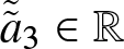 $\tilde{\tilde{a}}_3 \in \mathbb{R}$ is a new parameter. For the second equation of system (A.6), we compute
 \begin{align*}
\mathcal{L}_1 \hat{v}_1 + \mathcal{L}_2 \hat{v}_0 &= -4 a_1 [\sin(3u) + \sin(u)] - 4 a_2 [\cos(3u) + \cos(u)] + 2 a_2 \cos(u) \\
& \quad + 2 [a_1 \sin(u) + a_2 \cos(u)] - 2a_1 [\sin(3u)-\sin(u)] - 2 a_2 [\cos(3u) + \cos(u)]
\end{align*}
whereas  $\mathcal{H}_{\pm} \hat{v}_1$ and
 $\mathcal{L}_{\pm}^{(1)} \hat{v}_0$ only return projections to
 ${\rm span}(1,\sin(2u),\cos(2u))$. Projecting the second equation of system (A.6) to
 ${\rm Ker}(\mathcal{K}-1) = {\rm span}(\sin(u),\cos(u))$ yields the linear system
 \begin{equation*}
\left[ \begin{matrix} \lambda_1^2 & 2 \lambda_2 \\ -2 \lambda_2 & \lambda_1^2 + 2 \end{matrix} \right]
\left[ \begin{matrix} a_1 \\ a_2 \end{matrix} \right] = \left[ \begin{matrix} 0 \\ 0 \end{matrix} \right],
\end{equation*}
which admits a nontrivial solution for 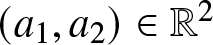 $(a_1,a_2) \in \mathbb{R}^2$ if and only if
 \begin{equation}
\lambda_2^2 = -\frac{1}{4} \lambda_1^2 (2 + \lambda_1^2) = \frac{1}{64} \mu_1^2 (8 - \mu_1^2).
\end{equation}
Combining (A.5) and (A.7) into (A.2) yields the characteristic equation (A.1). Since the spectral bands given by (A.1) are non-degenerate, persistence of the asymptotic expansion (A.3) follows from [Reference Hinch25, Reference Hormander26, Reference Kirwan28].
Remark 22. There exist two additional spectral bands of the modulational stability problem (1.27) near the origin associated with the subspace  ${\rm Ker}(\mathcal{K}) = {\rm span}(1)$. Similar to the proof of the second part of Theorem 1, the two spectral bands are subsets of
 $i \mathbb{R}$ associated with the scaling
 $\mu = a^2 \mu_2$ and
 $\lambda = a \lambda_1 + \mathcal{O}(a^2)$.
Appendix B. Numerical methods
For numerical approximations, we compute the profile of the smooth Stokes waves from the pseudo–differential equation (1.11) and solve the modulational stability problem (1.27).
B.1. Finding the Stokes wave
Finding Stokes waves to high accuracy is a delicate problem that has been studied in detail [Reference Dyachenko, Hur and Silantyev21, Reference Dyachenko, Lushnikov and Korotkevich22, Reference Korotkevich, Lushnikov, Semenova and Dyachenko29]. The goal is to determine a nontrivial pair 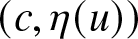 $(c,\eta(u))$, that satisfies the pseudo-differential equation,
 \begin{equation}
\left(c^2 \mathcal{K} - 1 \right) \eta - \left( \eta \mathcal{K}\eta + \frac{1}{2}\mathcal{K} \eta^2 \right) = 0.
\end{equation}
Due to the  $2\pi$-periodicity and evenness of
 $\eta = \eta(u)$, we use the truncated Fourier series,
 \begin{equation}
\eta(u) = \sum\limits_{|k| \leq N/2} \hat{\eta}_k e^{iku},
\end{equation}
with  $\hat{\eta}_k \in \mathbb{R}$,
 $\forall k$ and
 $N$ is the number of Fourier modes in the truncated approximation (B.2). The problem (B.1) is solved by Newton’s method coupled with a minimal residual (MINRES) method. The key idea is to take an approximate solution from the linear limit, or a previously computed solution pair, given by
 $(c^{(j)},\eta^{(j)}(u))$, and apply the continuation method in the
 $c$ parameter. The wave speed is adjusted to
 $c^{(j+1)} = c^{(j)} + \delta c^{(j)}$, where
 $\delta c^{(j)}$ is variable, and the solution,
 $\eta^{(j)}(u)$, from the preceding step,
 $j$, is used to initialize Newton iterations on equation (B.1). After convergence, we obtain
 $(c^{(j+1)},\eta^{(j+1)})$ with a prescribed tolerance, and the next step of the continuation method is applied. Once the Stokes wave is found, we define its steepness,
 $s = (\eta(0) - \eta(\pi))/2\pi$, or equivalently the ratio of crest to trough height to one wavelength, as well as its integral characteristics, like
 $\mathcal{H}(c)$,
 $\mathcal{P}(c)$ and
 $\mathcal{N}(c)$. It becomes convenient to present speed and integral characteristics as functions of
 $s$ due to their oscillations in
 $s$.
The method of continuation generally fails at a fold point  $c_0 = c(s_0)$, where the linearized operator
 $\mathcal{L} : H^1_{\rm per} \subset L^2_{\rm per} \to L^2_{\rm per}$ is not invertible on the space of even functions, associated with the bifurcation in Section 7. In any small neighbourhood of
 $|c-c_0|\leq \delta $, there may exist two distinct solutions of equation (B.1) with the same value of speed. This technical difficulty is mitigated by perturbing the initial guess for Newton’s method, and allows us to cross fold points by exploiting basins of attraction of solutions on both sides of the fold point.
B.2. Finding eigenvalues
Once the Stokes wave has been determined, its linear stability is determined by the eigenvalues of the modulational stability problem
 \begin{equation}
\begin{cases}
\mathcal{K} w = \lambda \mathcal{M} v, \\
\mathcal{L} v = \lambda \left( \mathcal{M}^*w - 2c\mathcal{H}v \right),
\end{cases}
\end{equation}
where  $\mathcal{L}$ is the linearized Babenko operator (1.16),
 $(v,w) \in H^1(\mathbb{R}) \times H^1(\mathbb{R})$ is an eigenfunction, and
 $\lambda$ is the eigenvalue. By Fourier–Floquet theory, the spectral problem (B.3) can be solved by using the truncated Fourier series,
 \begin{equation}
\begin{cases}
w(u) = e^{i\mu u} \sum\limits_{|k| \leq N/2} \hat{w}_k e^{iku}, \\
v(u) = e^{i\mu u} \sum\limits_{|k| \leq N/2} \hat{v}_k e^{iku},
\end{cases}
\end{equation}
where the Floquet parameter,  $\mu\in[-\frac{1}{2},\frac{1}{2})$ is introduced. We discretize the interval
 $\mu\in[-\frac{1}{2}, \frac{1}{2}]$ on a grid to approximate
 $\lambda_j =\lambda_j(\mu)$ for each eigenvalue of (B.3) out of the handful of eigenvalues nearest to zero in the
 $\lambda$-plane. We refer the reader to [Reference Dyachenko and Semenova23, Reference Dyachenko and Semenova24] for a complete recipe of the numerical solution of (B.3) with (B.4), but simply note that the eigenvalue problem is solved via a matrix-free orthogonal projection method, where the linear system is solved via minimal residual (MINRES) iterations.

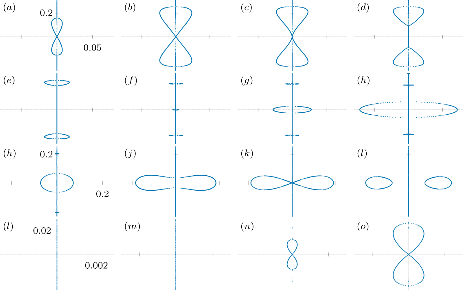

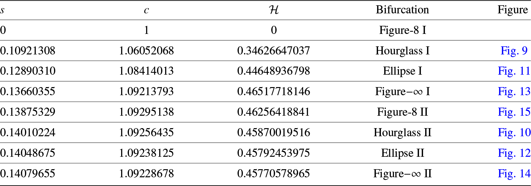


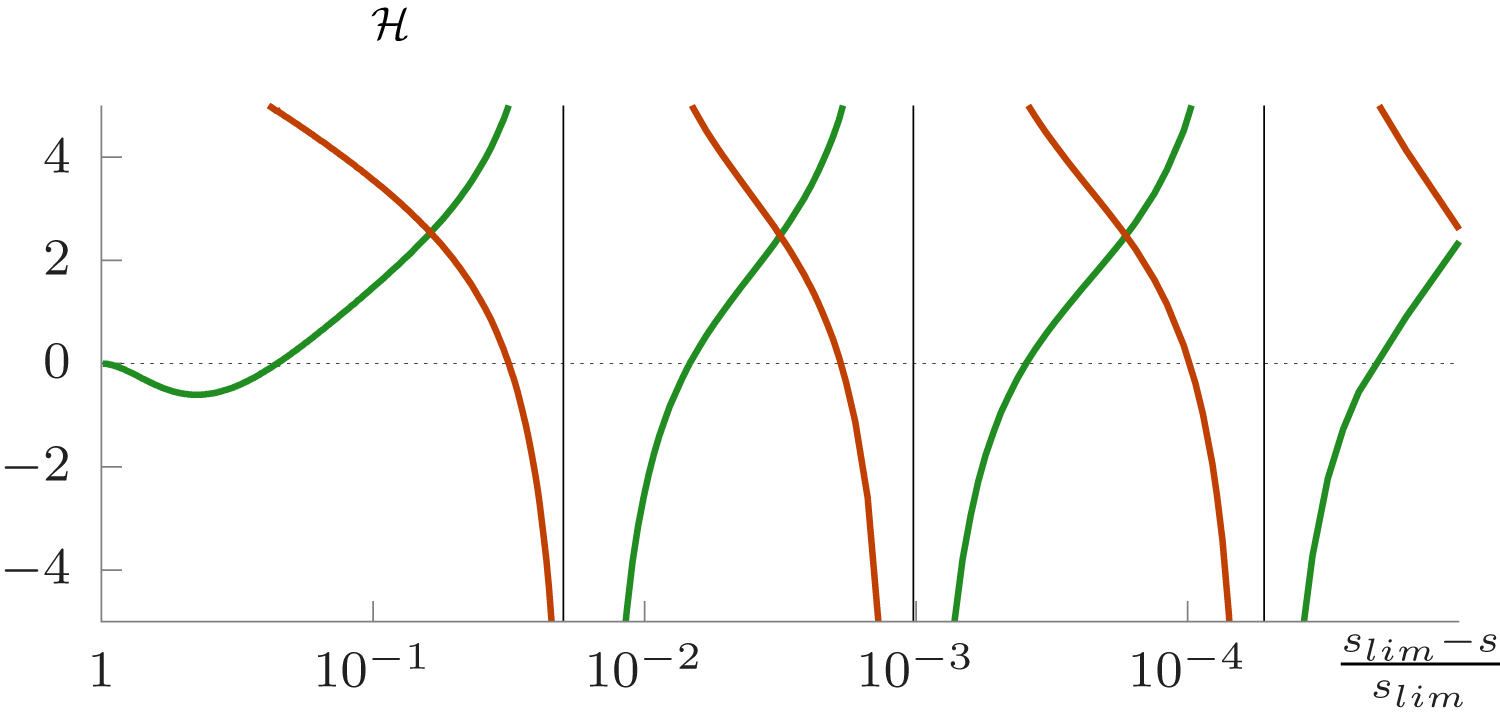


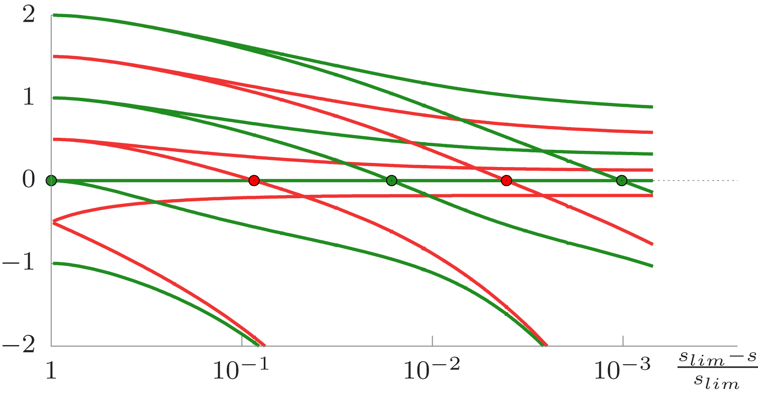

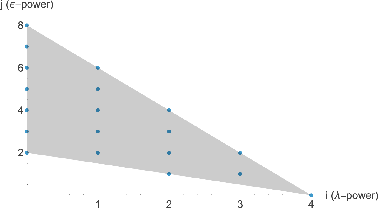


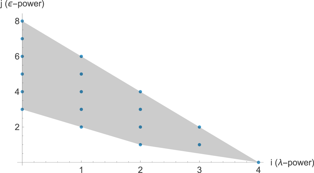


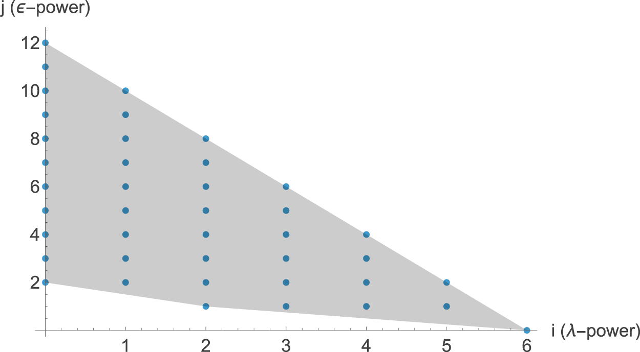


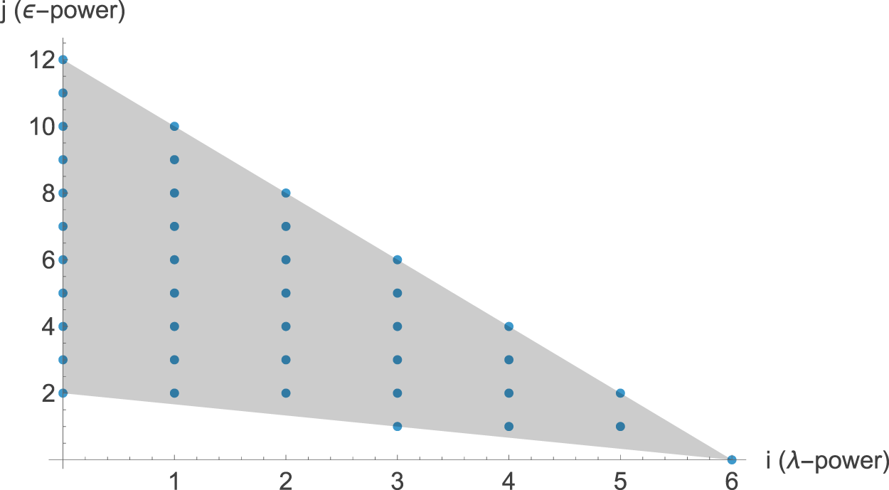


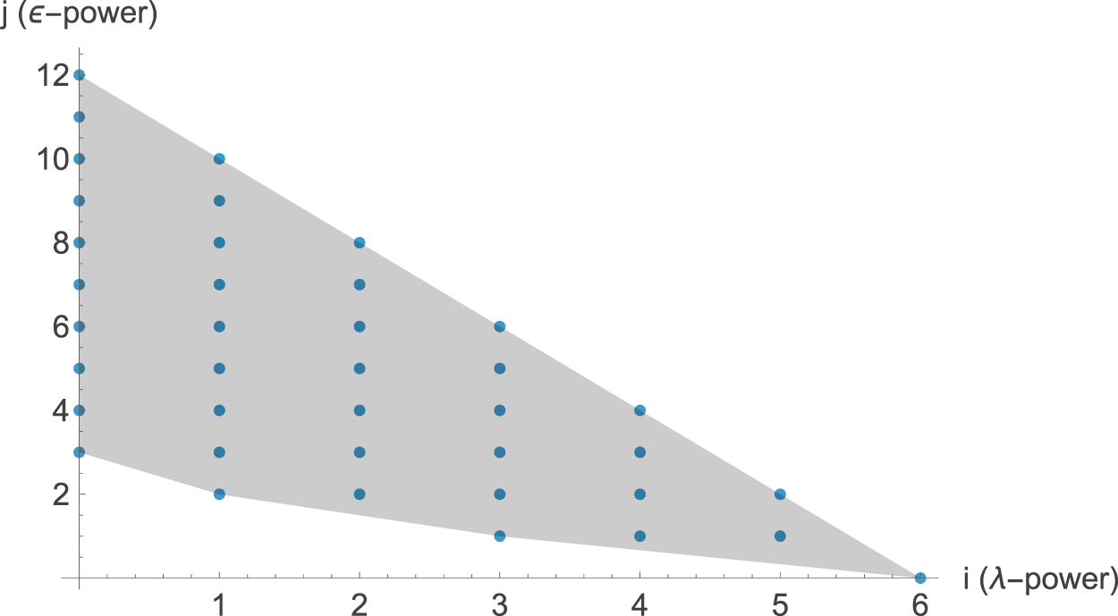



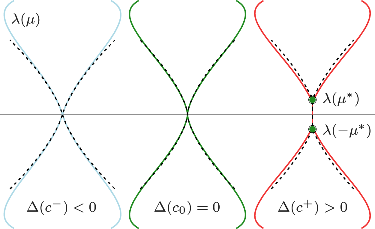


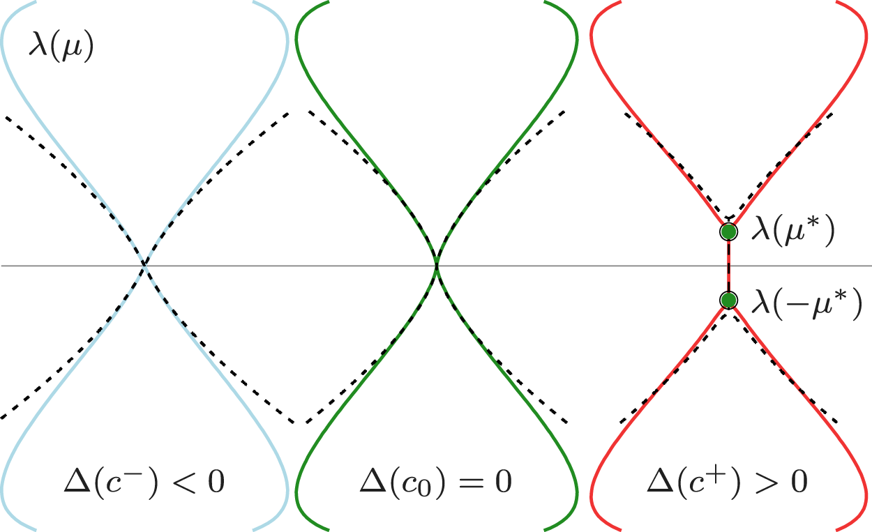



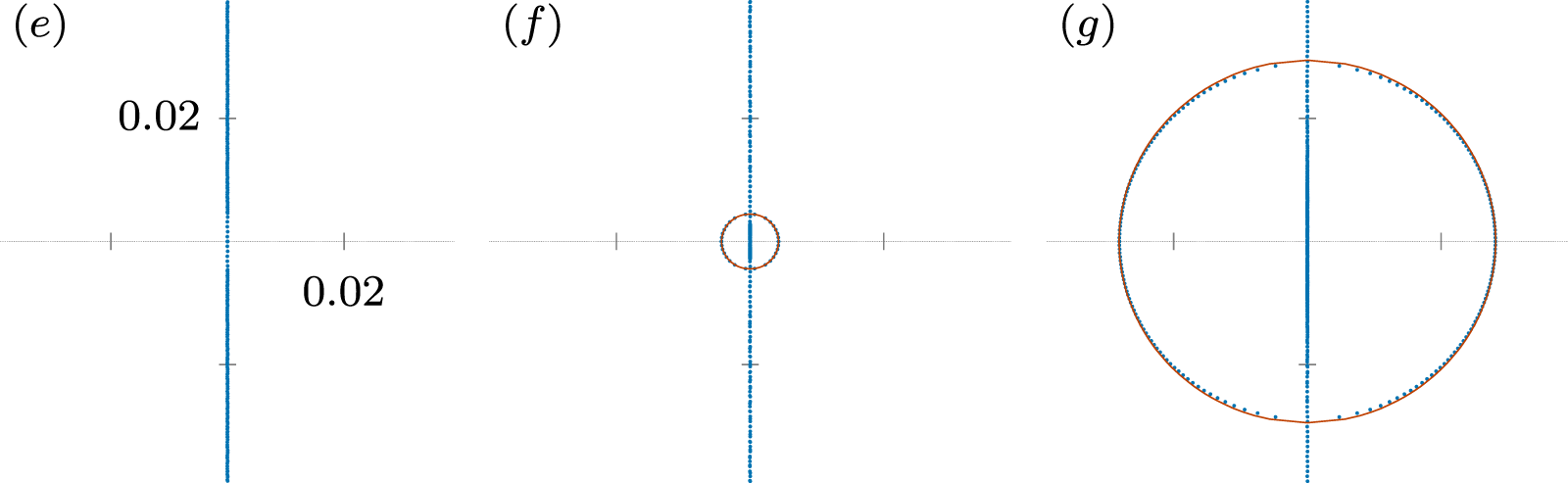


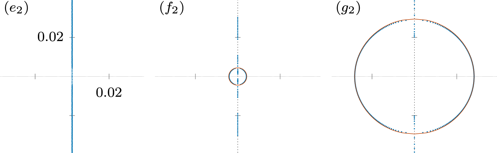




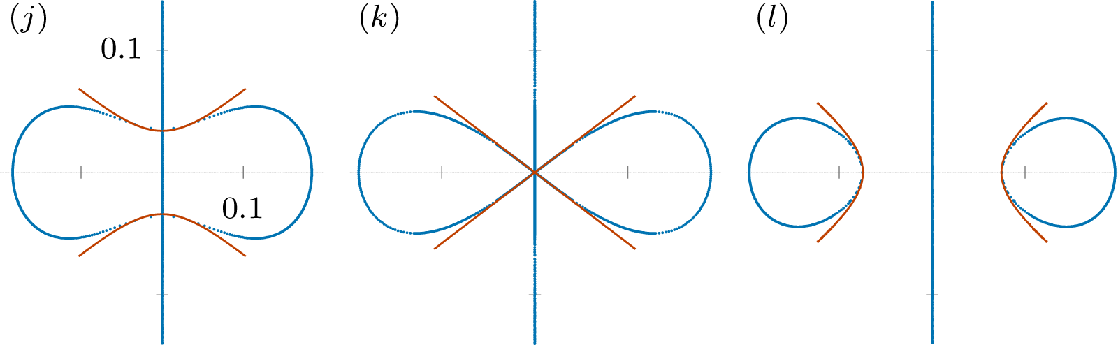


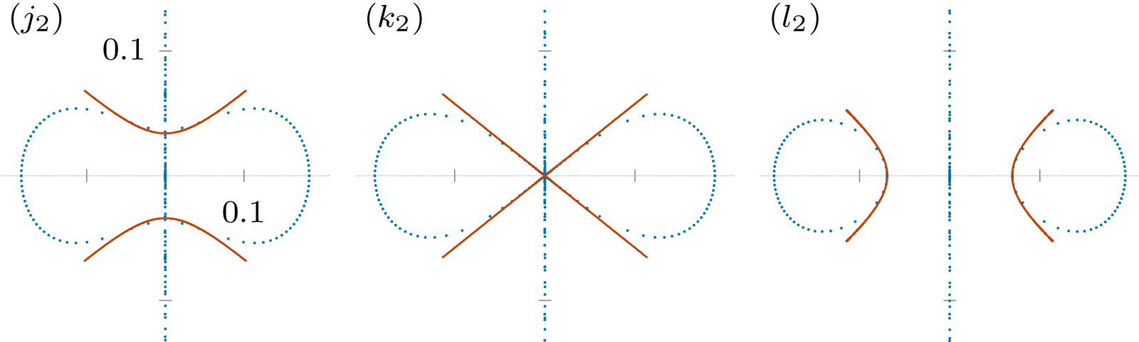




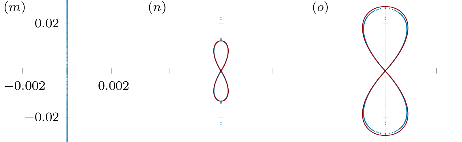


 Open access

