2 Stability problem formulation

The general framework and governing equations of the problem are discussed in Part 1, where the sketch of the channel flow is given in figure 1 and whose notations and definitions we adopt here. The governing equations for this problem are found in Frenkel, Halpern & Schweiger (Reference Frenkel, Halpern and Schweiger2018) as well. For convenience, we reproduce some of the more important ones below, in this section and the next one. In particular, we assume the dependence of surface tension $\unicode[STIX]{x1D70E}^{\ast }$ on the surfactant concentration $\unicode[STIX]{x1D6E4}^{\ast }$ , where the star superscript indicates dimensional variables, to be given by the Langmuir isotherm relation (Edwards, Brenner & Wasan Reference Edwards, Brenner and Wasan1991), which for the small disturbances is

(2.1) $$\begin{eqnarray}\unicode[STIX]{x1D70E}^{\ast }=\unicode[STIX]{x1D70E}_{0}-E(\unicode[STIX]{x1D6E4}^{\ast }-\unicode[STIX]{x1D6E4}_{0}),\end{eqnarray}$$

where $\unicode[STIX]{x1D70E}_{0}$ is the undisturbed surface tension, $\unicode[STIX]{x1D6E4}_{0}$ is the corresponding surfactant concentration and $E:=-(\unicode[STIX]{x2202}\unicode[STIX]{x1D70E}^{\ast }/\unicode[STIX]{x2202}\unicode[STIX]{x1D6E4}^{\ast })|_{\unicode[STIX]{x1D6E4}^{\ast }=\unicode[STIX]{x1D6E4}_{0}}$ is the elasticity parameter.

We make use of the following dimensionless variables:

(2.2a-c ) $$\begin{eqnarray}(x,z,\unicode[STIX]{x1D702})=\frac{(x^{\ast },z^{\ast },\unicode[STIX]{x1D702}^{\ast })}{d_{1}},\quad t=\frac{t^{\ast }}{d_{1}\unicode[STIX]{x1D707}_{1}/\unicode[STIX]{x1D70E}_{0}},\quad \boldsymbol{v}_{j}=(u_{j},w_{j})=\frac{(u_{j}^{\ast },w_{j}^{\ast })}{\unicode[STIX]{x1D70E}_{0}/\unicode[STIX]{x1D707}_{1}},\end{eqnarray}$$

(2.3a-c ) $$\begin{eqnarray}p_{j}=\frac{p_{j}^{\ast }}{\unicode[STIX]{x1D70E}_{0}/d_{1}},\quad \unicode[STIX]{x1D6E4}=\frac{\unicode[STIX]{x1D6E4}^{\ast }}{\unicode[STIX]{x1D6E4}_{0}},\quad \unicode[STIX]{x1D70E}=\frac{\unicode[STIX]{x1D70E}^{\ast }}{\unicode[STIX]{x1D70E}_{0}}.\end{eqnarray}$$

The base velocity and pressure profiles in the two layers separated by a flat interface, $\unicode[STIX]{x1D702}=0$ , having a uniform surfactant distribution $\bar{\unicode[STIX]{x1D6E4}}=1$ and a constant surface tension $\bar{\unicode[STIX]{x1D70E}}=1$ (using the over-bar for all base quantities), are (Frenkel & Halpern Reference Frenkel and Halpern2017)

(2.4a-c ) $$\begin{eqnarray}\bar{u}_{1}(z)=sz,\quad \bar{w}_{1}=0,\quad \text{and}\quad \bar{p}_{1}=-Bo_{1}z\quad \text{for}~-1\leqslant z\leqslant 0.\end{eqnarray}$$

(2.5a-c ) $$\begin{eqnarray}\bar{u_{2}}(z)=\frac{s}{m}z,\quad \bar{w}_{2}=0,\quad \text{and}\quad \bar{p}_{2}=-Bo_{2}z\quad \text{for}~0\leqslant z\leqslant n,\end{eqnarray}$$

where $Bo_{j}:=\unicode[STIX]{x1D70C}_{j}gd_{1}^{2}/\unicode[STIX]{x1D70E}_{0}$ is the Bond number of layer $j$ , $m=\unicode[STIX]{x1D707}_{2}/\unicode[STIX]{x1D707}_{1}$ is the viscosity ratio and $n=d_{2}/d_{1}$ is the ratio of the thicknesses of the two layers. The base interfacial shear rate of the bottom layer, $s=D\bar{u}_{1}(0)$ (where $D=\text{d}/\text{d}z$ ), is used to characterize the base flow instead of $U=\unicode[STIX]{x1D707}_{1}U^{\ast }/\unicode[STIX]{x1D70E}_{0}=s(1+n/m)$ , the relative velocity of the plates. We express the disturbed state with small deviations from the base flow as follows:

(2.6a-d ) $$\begin{eqnarray}\unicode[STIX]{x1D702}=\tilde{\unicode[STIX]{x1D702}}\cdot u_{j}=\bar{u}_{j}+\tilde{u} _{j},\quad w_{j}=\tilde{w}_{j},\quad p_{j}=\bar{p}_{j}+\tilde{p}_{j},\quad \unicode[STIX]{x1D6E4}=\bar{\unicode[STIX]{x1D6E4}}+\tilde{\unicode[STIX]{x1D6E4}}.\end{eqnarray}$$

The normal modes are disturbances of the form

(2.7) $$\begin{eqnarray}(\tilde{\unicode[STIX]{x1D702}},\tilde{u} _{j},\tilde{w}_{j},\tilde{p}_{j},\tilde{\unicode[STIX]{x1D6E4}})=[h,\hat{u} _{j}(z),{\hat{w}}_{j}(z),\hat{f}_{j}(z),G]\text{e}^{\text{i}\unicode[STIX]{x1D6FC}x+\unicode[STIX]{x1D6FE}t},\end{eqnarray}$$

where $\hat{u} _{j}(z)$ , ${\hat{w}}_{j}(z)$ and $\hat{f}_{j}(z)$ are complex amplitudes, $\unicode[STIX]{x1D6FC}$ is the wavenumber, $G$ and $h$ are constant amplitudes and $\unicode[STIX]{x1D6FE}$ is the increment, $\unicode[STIX]{x1D6FE}=\unicode[STIX]{x1D6FE}_{R}+\text{i}\unicode[STIX]{x1D6FE}_{I}$ . The flow stability depends on the sign of the growth rate $\unicode[STIX]{x1D6FE}_{R}=\text{Re}(\unicode[STIX]{x1D6FE})$ : the flow is unstable if $\unicode[STIX]{x1D6FE}_{R}>0$ for some normal modes; and it is stable if $\unicode[STIX]{x1D6FE}_{R}<0$ for all normal modes. The linearized governing equations for the disturbances translate into a system for the amplitudes. Using the continuity equations, the horizontal velocity amplitudes $\hat{u} _{j}$ are eliminated in terms of ${\hat{w}}_{j}$ . The pressure disturbances are eliminated from the momentum equations, in which inertia has been neglected, and we obtain the Orr–Sommerfeld equations for the vertical velocity disturbances:

(2.8) $$\begin{eqnarray}m_{j}(D^{2}-\unicode[STIX]{x1D6FC}^{2})^{2}{\hat{w}}_{j}=0,\end{eqnarray}$$

where $m_{j}:=\unicode[STIX]{x1D707}_{j}/\unicode[STIX]{x1D707}_{1}$ (so that $m_{1}=1$ and $m_{2}=m$ ). The boundary conditions at the plates are

(2.9a-d ) $$\begin{eqnarray}D{\hat{w}}_{1}(-1)=0,\quad {\hat{w}}_{1}(-1)=0,\quad D{\hat{w}}_{2}(n)=0,\quad {\hat{w}}_{2}(n)=0.\end{eqnarray}$$

The kinematic boundary condition and surfactant transport equation, respectively, take the forms

(2.10) $$\begin{eqnarray}\unicode[STIX]{x1D6FE}h-{\hat{w}}_{1}=0\quad (z=0)\end{eqnarray}$$

and

(2.11) $$\begin{eqnarray}\unicode[STIX]{x1D6FE}G-D{\hat{w}}_{1}+s\text{i}\unicode[STIX]{x1D6FC}h=0\quad (z=0).\end{eqnarray}$$

Continuity of velocity at the interface gives rise to

(2.12) $$\begin{eqnarray}{\hat{w}}_{1}-{\hat{w}}_{2}=0\quad (z=0)\end{eqnarray}$$

and

(2.13) $$\begin{eqnarray}D{\hat{w}}_{2}-D{\hat{w}}_{1}-\text{i}\unicode[STIX]{x1D6FC}sh\left(\frac{1-m}{m}\right)=0\quad (z=0).\end{eqnarray}$$

The interfacial tangential and normal stress conditions yield, respectively,

(2.14) $$\begin{eqnarray}mD^{2}{\hat{w}}_{2}-D^{2}{\hat{w}}_{1}+\unicode[STIX]{x1D6FC}^{2}(m{\hat{w}}_{2}-{\hat{w}}_{1})-\unicode[STIX]{x1D6FC}^{2}GMa=0\quad (z=0)\end{eqnarray}$$

and (eliminating the pressure disturbances in terms of ${\hat{w}}_{j}$ by using the horizontal momentum equations)

(2.15) $$\begin{eqnarray}mD^{3}{\hat{w}}_{2}-3m\unicode[STIX]{x1D6FC}^{2}D{\hat{w}}_{2}-D^{3}{\hat{w}}_{1}+Bo\unicode[STIX]{x1D6FC}^{2}h+3\unicode[STIX]{x1D6FC}^{2}D{\hat{w}}_{1}+\unicode[STIX]{x1D6FC}^{4}h=0\quad (z=0),\end{eqnarray}$$

where $Ma:=E\unicode[STIX]{x1D6E4}_{0}/\unicode[STIX]{x1D70E}_{0}$ is the Marangoni number and $Bo$ is the effective Bond number

(2.16) $$\begin{eqnarray}Bo=Bo_{1}-Bo_{2}=\frac{(\unicode[STIX]{x1D70C}_{1}-\unicode[STIX]{x1D70C}_{2})gd_{1}^{2}}{\unicode[STIX]{x1D70E}_{0}},\end{eqnarray}$$

which can be negative, unlike the parameters $n$ , $m$ , $s$ and $Ma$ . Equations (2.8)–(2.13), (2.14) and (2.15) form the eigenvalue boundary value problem for the disturbances, which determines the growth rate as a function of the wavenumber $\unicode[STIX]{x1D6FC}$ and the parameters $s$ , $m$ , $n$ , $Ma$ and $Bo$ . The eigenvalue, the increment $\unicode[STIX]{x1D6FE}$ , satisfies a quadratic equation which appears in the next section.

3 Dispersion relation; special points of dispersion curves

In this section, we include a shortened version of the derivation of the dispersion equation for the increment $\unicode[STIX]{x1D6FE}$ and provide some other important equations. (See Part 1 for more details.) The general solutions of (2.8) are

(3.1) $$\begin{eqnarray}{\hat{w}}_{j}(z)=a_{j}\cosh (\unicode[STIX]{x1D6FC}z)+b_{j}\sinh (\unicode[STIX]{x1D6FC}z)+c_{j}z\cosh (\unicode[STIX]{x1D6FC}z)+d_{j}z\sinh (\unicode[STIX]{x1D6FC}z),\end{eqnarray}$$

where $a_{j}$ , $b_{j}$ , $c_{j}$ and $d_{j}$ are determined by the boundary conditions. First, we apply (2.12) which yields $a_{2}=a_{1}$ , and then by applying the plate velocity conditions, equation (2.9), we can express $c_{1}$ and $d_{1}$ in terms of $a_{1}$ and $b_{1}$ , and $c_{2}$ and $d_{2}$ in terms of $a_{1}$ and $b_{2}$ , so that the velocity expressions are

(3.2) $$\begin{eqnarray}\displaystyle {\hat{w}}_{1}(z) & = & \displaystyle a_{1}\cosh (\unicode[STIX]{x1D6FC}z)+b_{1}\sinh (\unicode[STIX]{x1D6FC}z)+\frac{1}{\unicode[STIX]{x1D6FC}}[-s_{\unicode[STIX]{x1D6FC}}^{2}b_{1}+\left(s_{\unicode[STIX]{x1D6FC}}c_{\unicode[STIX]{x1D6FC}}+\unicode[STIX]{x1D6FC}\right)a_{1}]z\cosh (\unicode[STIX]{x1D6FC}z)\nonumber\\ \displaystyle & & \displaystyle +\,\frac{1}{\unicode[STIX]{x1D6FC}}[-(s_{\unicode[STIX]{x1D6FC}}c_{\unicode[STIX]{x1D6FC}}-\unicode[STIX]{x1D6FC})b_{1}+c_{\unicode[STIX]{x1D6FC}}^{2}a_{1}]z\sinh (\unicode[STIX]{x1D6FC}z)\end{eqnarray}$$

and

(3.3) $$\begin{eqnarray}\displaystyle {\hat{w}}_{2}(z) & = & \displaystyle a_{1}\cosh (\unicode[STIX]{x1D6FC}z)+b_{2}\sinh (\unicode[STIX]{x1D6FC}z)-\frac{1}{\unicode[STIX]{x1D6FC}n^{2}}[s_{\unicode[STIX]{x1D6FC}n}^{2}b_{2}+(s_{\unicode[STIX]{x1D6FC}n}c_{\unicode[STIX]{x1D6FC}n}+\unicode[STIX]{x1D6FC}n)a_{1}]z\cosh (\unicode[STIX]{x1D6FC}z)\nonumber\\ \displaystyle & & \displaystyle +\,\frac{1}{\unicode[STIX]{x1D6FC}n^{2}}[(s_{\unicode[STIX]{x1D6FC}n}c_{\unicode[STIX]{x1D6FC}n}-\unicode[STIX]{x1D6FC}n)b_{2}+c_{\unicode[STIX]{x1D6FC}n}^{2}a_{1}]z\sinh (\unicode[STIX]{x1D6FC}z),\end{eqnarray}$$

where

(3.4a-d ) $$\begin{eqnarray}c_{\unicode[STIX]{x1D6FC}}=\cosh (\unicode[STIX]{x1D6FC}),\quad s_{\unicode[STIX]{x1D6FC}}=\sinh (\unicode[STIX]{x1D6FC}),\quad c_{\unicode[STIX]{x1D6FC}n}=\cosh (\unicode[STIX]{x1D6FC}n),\quad s_{\unicode[STIX]{x1D6FC}n}=\sinh (\unicode[STIX]{x1D6FC}n).\end{eqnarray}$$

We obtain a linear non-homogeneous system for $a_{1}$ , $b_{1}$ and $b_{2}$ by substituting the above velocity expressions into the interfacial conditions (2.13), (2.14) and (2.15), which is then solved to obtain $a_{1}$ , $b_{1}$ and $b_{2}$ in terms of $h$ and $G$ . Then we can express the velocities ${\hat{w}}_{j}(z)$ in terms of $h$ and $G$ . The kinematic boundary condition (2.10) and the surfactant transport equation (2.11) give rise to a linear homogeneous system for $h$ and $G$ ,

(3.5) $$\begin{eqnarray}\left[\begin{array}{@{}cc@{}}(\unicode[STIX]{x1D6FE}+A_{11}) & A_{12}\\ A_{21} & (\unicode[STIX]{x1D6FE}+A_{22})\end{array}\right]\left[\begin{array}{@{}c@{}}h\\ G\end{array}\right]=\left[\begin{array}{@{}c@{}}0\\ 0\end{array}\right],\end{eqnarray}$$

where $A_{11}$ , $A_{12}$ , $A_{21}$ and $A_{22}$ are functions of the wavenumber $\unicode[STIX]{x1D6FC}$ and the system parameters given in appendix A. Non-trivial solutions exist only if $\det (A)=(\unicode[STIX]{x1D6FE}+A_{11})(\unicode[STIX]{x1D6FE}+A_{22})-A_{12}A_{21}=0$ , which yields a quadratic equation for the increment  $\unicode[STIX]{x1D6FE}$ ,

(3.6) $$\begin{eqnarray}F_{2}\unicode[STIX]{x1D6FE}^{2}+F_{1}\unicode[STIX]{x1D6FE}+F_{0}=0.\end{eqnarray}$$

Its solutions are given by

(3.7) $$\begin{eqnarray}\unicode[STIX]{x1D6FE}=\frac{1}{2F_{2}}(-F_{1}+[F_{1}^{2}-4F_{2}F_{0}]^{1/2}),\end{eqnarray}$$

where the expressions for $F_{2}$ , $F_{1}$ and $F_{0}$ in terms of system parameters and $\unicode[STIX]{x1D6FC}$ are given by (3.8)–(3.13) in Part 1, in which some of their properties are also enumerated. The ranges of the system parameters are documented there as well. In particular, we only need to consider $n\geqslant 1$ , but allow for $-\infty <Bo<\infty$ . As discussed in detail in Part 1, there are two continuous branches of the increment, given by $\unicode[STIX]{x1D6FE}$ (3.7), as a function of $\unicode[STIX]{x1D6FC}$ and the parameters, and correspondingly two continuous branches of the growth rate $\unicode[STIX]{x1D6FE}_{R}$ . The branch that is non-zero at $Ma=0$ is called the ‘robust branch’, and the other one, that vanishes as $Ma\downarrow 0$ , is the ‘surfactant branch’.

We will use the following equations for obtaining the maximum growth rate $\unicode[STIX]{x1D6FE}_{R\,max}$ , the wavenumber $\unicode[STIX]{x1D6FC}_{max}$ corresponding to the maximum growth rate and the marginal wavenumber $\unicode[STIX]{x1D6FC}_{0}$ (see also Part 1). The real and imaginary parts of the dispersion equation yield two real equations quadratic in $\unicode[STIX]{x1D6FE}_{R}$ and $\unicode[STIX]{x1D6FE}_{I}$ . Eliminating from them $\unicode[STIX]{x1D6FE}_{I},$ we obtain a quartic equation for $\unicode[STIX]{x1D6FE}_{R}$ :

(3.8) $$\begin{eqnarray}\displaystyle & & \displaystyle 4\,F_{2}^{3}\unicode[STIX]{x1D6FE}_{R}^{4}+8F_{2}^{2}\text{Re}(F_{1})\unicode[STIX]{x1D6FE}_{R}^{3}+F_{2}[4\,F_{2}\text{Re}(F_{0})+\text{Im}(F_{1})^{2}+5\,\text{Re}(F_{1})^{2}]\unicode[STIX]{x1D6FE}_{R}^{2}\nonumber\\ \displaystyle & & \displaystyle \qquad +\,\text{Re}(F_{1})[\text{Re}(F_{1})^{2}+4F_{2}\text{Re}(F_{0})+\text{Im}(F_{1})^{2}]\unicode[STIX]{x1D6FE}_{R}-F_{2}\text{Im}(F_{0})^{2}\nonumber\\ \displaystyle & & \displaystyle \qquad +\,\text{Re}(F_{1})^{2}\text{Re}(F_{0})+\text{Re}(F_{1})\text{Im}(F_{1})\text{Im}(F_{0})=0.\end{eqnarray}$$

Since $\unicode[STIX]{x1D6FE}_{R}=0$ at the marginal wavenumber, $\unicode[STIX]{x1D6FC}_{0}$ , only the last term in this equation remains, and we arrive at the following marginal wavenumber equation in terms of system parameters and $\unicode[STIX]{x1D6FC}$ :

(3.9) $$\begin{eqnarray}k_{20}Ma^{2}+k_{11}MaB+k_{31}Ma^{3}B+k_{22}Ma^{2}B^{2}+k_{13}MaB^{3}=0,\end{eqnarray}$$

where $B:=Bo+\unicode[STIX]{x1D6FC}^{2}$ and the coefficients $k_{ij}$ are functions of $\unicode[STIX]{x1D6FC}$ , $m$ , $n$ and $s$ (given explicitly in Frenkel et al. (Reference Frenkel, Halpern and Schweiger2018)).

For $Ma=0$ , equation (3.9) cannot be used. However, the only non-trivial solution of (3.6) for $Ma=0$ is $\unicode[STIX]{x1D6FE}=-F_{1}/F_{2}$ (since $F_{0}=0$ ), corresponding to the Rayleigh–Taylor instability mode. Hence, for the marginal wavenumber, we have $\text{Re}(F_{1})=0$ , which yields $\unicode[STIX]{x1D6FC}_{0}=(-Bo)^{1/2}$ provided $Bo<0$ .

The wavenumber $\unicode[STIX]{x1D6FC}_{max}$ and the maximum growth rate $\unicode[STIX]{x1D6FE}_{R\,max}$ are obtained by simultaneously solving (3.8) and the following equation which is obtained by differentiating (3.8) with respect to $\unicode[STIX]{x1D6FC}$ , taking into account that $\text{d}\unicode[STIX]{x1D6FE}_{R}/\text{d}\unicode[STIX]{x1D6FC}=0$ at the maximum:

(3.10) $$\begin{eqnarray}\unicode[STIX]{x1D6FE}_{R}^{4}\frac{\text{d}}{\text{d}\unicode[STIX]{x1D6FC}}C_{4}(\unicode[STIX]{x1D6FC})+\unicode[STIX]{x1D6FE}_{R}^{3}\frac{\text{d}}{\text{d}\unicode[STIX]{x1D6FC}}C_{3}(\unicode[STIX]{x1D6FC})+\unicode[STIX]{x1D6FE}_{R}^{2}\frac{\text{d}}{\text{d}\unicode[STIX]{x1D6FC}}C_{2}(\unicode[STIX]{x1D6FC})+\unicode[STIX]{x1D6FE}_{R}\frac{\text{d}}{\text{d}\unicode[STIX]{x1D6FC}}C_{1}(\unicode[STIX]{x1D6FC})+\frac{\text{d}}{\text{d}\unicode[STIX]{x1D6FC}}C_{0}(\unicode[STIX]{x1D6FC})=0,\end{eqnarray}$$

where $C_{j}$ denotes the coefficient of the $\unicode[STIX]{x1D6FE}_{R}^{j}$ term that appears in (3.8).

4 Surfactant effects in the $Q$ sector; mid-wave instability

It was shown in HF ( $Bo=0$ ) that for $Ma>5/2$ and $m>n^{2}$ (i.e. in the $Q$ sector; see figure 3 of Part 1 for the definition of the three sectors $Q$ , $R$ and $S$ ), there are mid-wave instability regimes, defined as those having a finite $\unicode[STIX]{x1D6FC}$ -interval, bounded away from $\unicode[STIX]{x1D6FC}=0$ , with $\unicode[STIX]{x1D6FE}_{R}>0$ for all its wavenumbers. (Note that the mid-wave instability was called type I in Cross & Hohenberg (Reference Cross and Hohenberg1993) while the long-wave instability was called type II.) In order to investigate such an instability allowing for non-zero Bond numbers, we introduce a critical Marangoni number, $Ma_{cM}$ that corresponds to the onset (or the turnoff) of the mid-wave instability, and let $\unicode[STIX]{x1D6FC}_{cM}$ be the corresponding wavenumber. Thus, the quantities $Ma_{cM}$ and $\unicode[STIX]{x1D6FC}_{cM}$ satisfy the equations $\unicode[STIX]{x1D6FE}_{R}=0$ and $\unicode[STIX]{x2202}\unicode[STIX]{x1D6FE}_{R}/\unicode[STIX]{x2202}\unicode[STIX]{x1D6FC}=0$ . In view of the quartic equation (3.8), $Ma_{cM}$ and $\unicode[STIX]{x1D6FC}_{cM}$ (for a given $Bo$ ) can be found by numerically solving (3.9), which we write in the notation used in (3.10) as

(4.1) $$\begin{eqnarray}C_{0}(Ma,\unicode[STIX]{x1D6FC},Bo)=0,\end{eqnarray}$$

along with

(4.2) $$\begin{eqnarray}\frac{\unicode[STIX]{x2202}}{\unicode[STIX]{x2202}\unicode[STIX]{x1D6FC}}C_{0}(Ma,\unicode[STIX]{x1D6FC},Bo)=0.\end{eqnarray}$$

To illustrate the change of stability with $Ma$ , in figure 1(a,b) the growth rate in the $Q$ sector (for $n=2$ and $m=5$ , at $s=1$ ) is plotted for three selected values of the Marangoni number and $Bo=-0.45$ . The numerical results show that the instability is a long-wave one provided $Ma<Ma_{cL}$ ( ${\approx}2.28$ for the figure parameters). This is then followed by a region of stability when $Ma\in [Ma_{cL},Ma_{cM}]$ , where $Ma_{cM}\approx 15.6$ . For $Ma_{cL}\,<Ma<Ma_{m}$ , $\unicode[STIX]{x1D6FE}_{R}$ decreases monotonically with $\unicode[STIX]{x1D6FC}$ (so that there is no $\unicode[STIX]{x1D6FE}_{R\,max}$ ; such dispersion curves are not shown in figure 1 b), but starting from $Ma_{m}$ ( ${\approx}3.70$ ), the local maximum $\unicode[STIX]{x1D6FE}_{R\,max}$ appears on the dispersion curves. So, the growth rate $\unicode[STIX]{x1D6FE}_{R}$ has a local (negative) maximum $\unicode[STIX]{x1D6FE}_{R\,max}$ at some $\unicode[STIX]{x1D6FC}_{max}>0~$ provided $Ma\geqslant Ma_{m}$ ; and once $Ma$ exceeds $Ma_{cM}$ , $\unicode[STIX]{x1D6FE}_{R\,max}$ becomes positive, i.e. the mid-wave instability switches on. Note that when $Ma>Ma_{cM}$ for at least some interval of $Ma$ corresponding to the mid-wave instability, there are two positive marginal wavenumbers, one on the left at $\unicode[STIX]{x1D6FC}=\unicode[STIX]{x1D6FC}_{0L}$ and another one on the right at $\unicode[STIX]{x1D6FC}=\unicode[STIX]{x1D6FC}_{0R}$ so that the interval of unstable wavenumbers is $\unicode[STIX]{x1D6FC}_{0L}<\unicode[STIX]{x1D6FC}<\unicode[STIX]{x1D6FC}_{0R}$ . (Cases with both finite and infinite $Ma$ intervals of mid-wave instability can be seen below in figure 7 a and are discussed in the last paragraph of § 5.3.)

Figure 1.

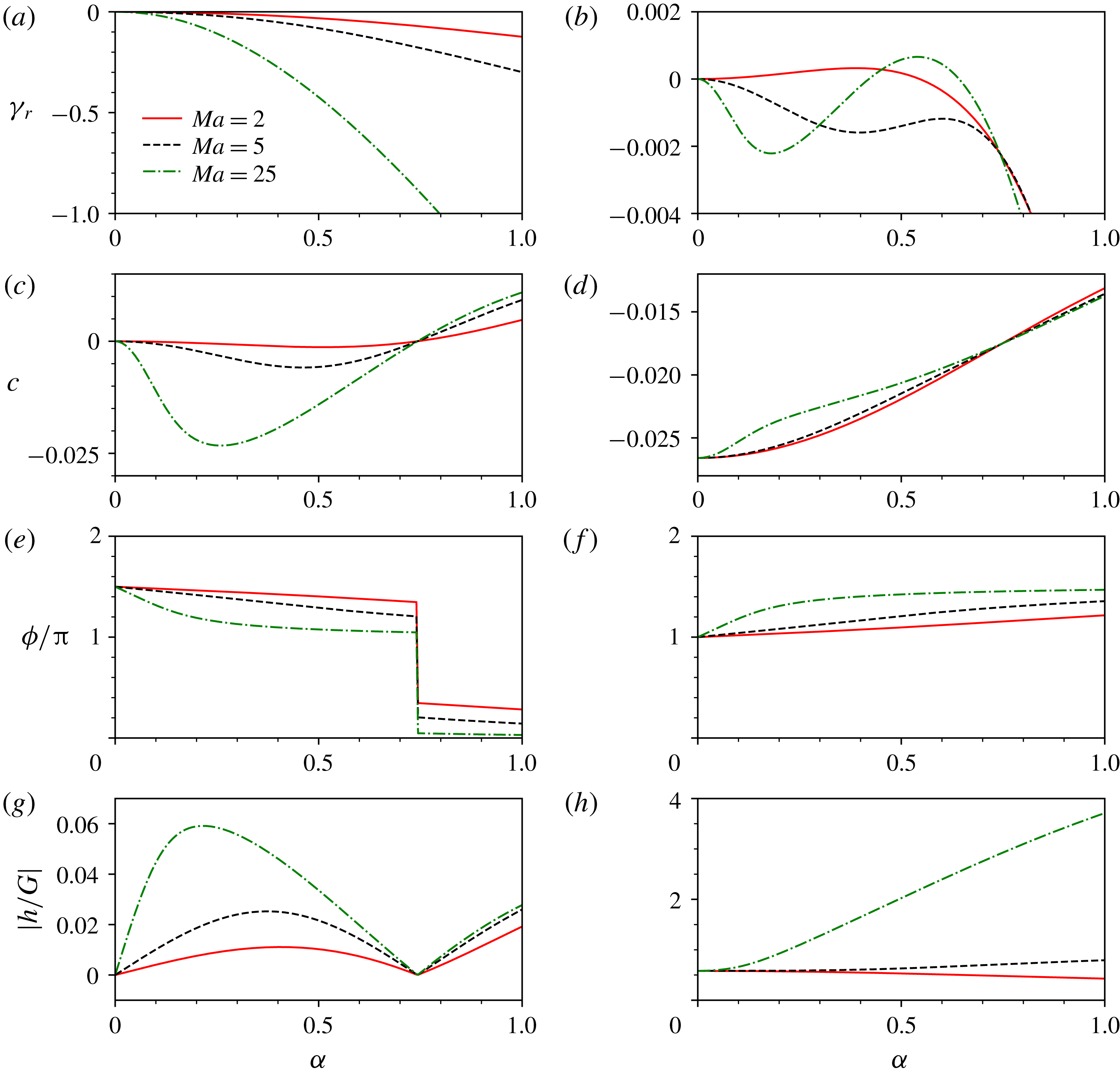
Curves for the four different functions of the wavenumber in the $Q$ sector ( $n=2$ , $m=5$ ) for $s=1$ and $Bo=-0.45$ . The stable mode corresponds to the panels of the left-hand column, and the less stable mode to the panels of the right-hand column. For the three values of $Ma$ given in the legend, panels (a,b) show the growth rates, (c,d) show the wave velocities, (e,f) show the interface–surfactant phase shifts and (g,h) show the interface/surfactant amplitude ratio. The transition from the long-wave instability to stability to the mid-wave instability as $Ma$ increases is evident in (b).

Although the stability properties of the normal modes are fully given by the dispersion curves (see figure 1 a,b), the normal modes have additional remarkable properties, such as the phase speed, the phase difference between the co-travelling waves of the interface and the surfactant, and the amplitude ratio of the interface to the surfactant disturbances. As an example, these quantities are plotted in figure 1 as functions of the wavenumber $\unicode[STIX]{x1D6FC}$ . There, one notices a special value of the wavenumber, $\unicode[STIX]{x1D6FC}_{s}$ , close to 0.7, at which the phase shift of the decaying branch has a jump discontinuity. The wave speed at $\unicode[STIX]{x1D6FC}_{s}$ is zero for any $Ma$ , so all three curves intersect at the same point $(\unicode[STIX]{x1D6FC}_{s},0)$ ; similarly, the amplitude ratio is zero, independent of $Ma$ . For the other branch, in the right-hand panels (which, as figure 1(b) shows, goes, as $Ma$ increases, from long-wave unstable, to stable and then to mid-wave unstable), all three growth rates are equal at the same $\unicode[STIX]{x1D6FC}_{s}$ , and the wave speeds are equal as well, but the amplitude ratios are non-zero and different.

These observations concerning the different quantities at the special value $\unicode[STIX]{x1D6FC}=\unicode[STIX]{x1D6FC}_{s}$ , which, in particular, imply the existence of normal modes with an undisturbed interface, $h=0$ , but $G\neq 0$ , are explained in appendix A. The question arises if there exist some ‘opposite’ modes, in which only the interface, but not the surfactant, is disturbed, so that $G=0$ , but $h\neq 0$ . We answer this in appendix B. It turns out that such modes are possible, but only in the absence of the basic interfacial shear of velocity, and that they are due to the Rayleigh–Taylor instability.

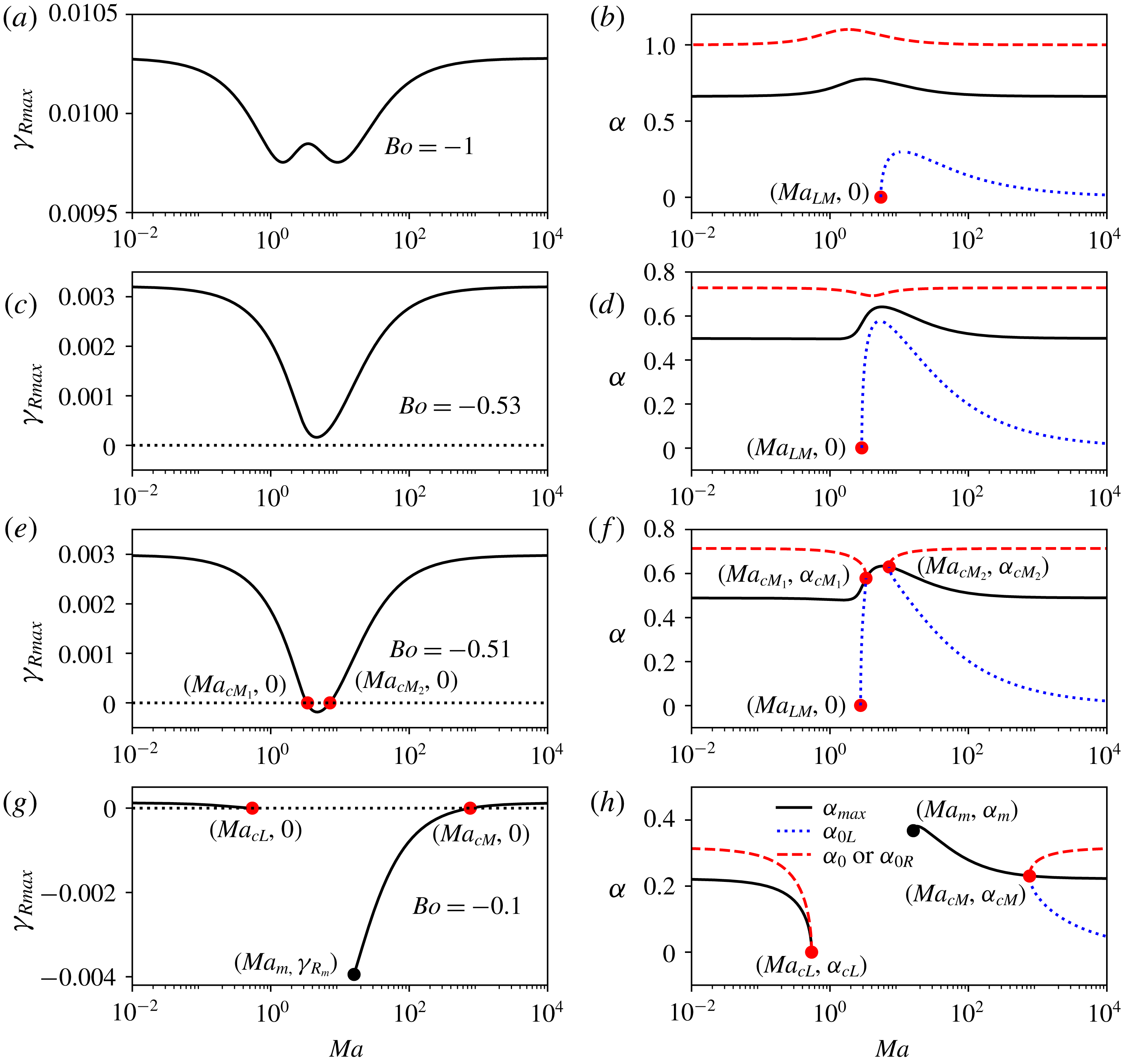
In figure 2, $\unicode[STIX]{x1D6FE}_{R\,max}$ , $\unicode[STIX]{x1D6FC}_{max}$ and $\unicode[STIX]{x1D6FC}_{0}$ are plotted versus the Marangoni number for $n=2$ , $m=5$ , $s=1$ and for four selected values of $Bo$ . If $Bo$ is sufficiently negative, as in figure 2(a,c), then $\unicode[STIX]{x1D6FE}_{R}>0$ for all $Ma$ .

Figure 2.

Plots of $\unicode[STIX]{x1D6FE}_{R\,max}$ (left-hand panels) and corresponding $\unicode[STIX]{x1D6FC}_{max}$ , $\unicode[STIX]{x1D6FC}_{0R}$ and $\unicode[STIX]{x1D6FC}_{0L}$ (right-hand panels) versus $Ma$ in the $Q$ sector (here at $n=2$ , $m=5$ ) for $s=1$ and the four indicated values of $Bo$ . (For labelled points, see the text.)

For $Ma<Ma_{LM}$ , the instability is a long-wave one; in other words, there is no $\unicode[STIX]{x1D6FC}_{0L}$ , since its definition implies that $\unicode[STIX]{x1D6FC}_{0L}$ must be non-zero. However, a mid-wave instability ensues when $Ma>Ma_{LM}$ , and there appears $\unicode[STIX]{x1D6FC}_{0L}>0$ (as in figure 2 b,d). Initially, $\unicode[STIX]{x1D6FC}_{0L}$ increases rapidly, while $\unicode[STIX]{x1D6FC}_{0R}$ decreases by a small amount, leading to the shrinkage of the interval of unstable wavenumbers. After reaching a maximum, $\unicode[STIX]{x1D6FC}_{0L}$ decreases towards zero with increasing $Ma$ but never attains the zero value so that the instability does not return to the long-wave type, and the interval of unstable wavenumbers slowly expands. When $Bo=-0.51$ (see figure 2 e,f), the stability picture up to $Ma=Ma_{cM_{1}}$ is very similar to that displayed in figure 2(b,d). The instability is of long-wave type provided $Ma<Ma_{LM}$ . Starting at $Ma=Ma_{LM}$ , corresponding to the lower left dot in figure 2(f), the long-wave instability disappears, and the mid-wave instability mentioned previously emerges. However, as $Ma$ continues to increase, the interval of unstable wavenumbers quickly shrinks to a single, non-zero, $\unicode[STIX]{x1D6FC}$ point, indicated by the dot at $Ma=Ma_{cM_{1}}$ . The flow then becomes stable, with $\unicode[STIX]{x1D6FE}_{R}<0$ for a range of Marangoni numbers, $Ma_{cM_{1}}<Ma<Ma_{cM_{2}}$ . Therefore, in this range, $\unicode[STIX]{x1D6FC}_{0L}$ and $\unicode[STIX]{x1D6FC}_{0R}$ are non-existent, but $\unicode[STIX]{x1D6FC}_{max}$ is defined because $\unicode[STIX]{x1D6FE}_{R}$ has a local maximum at a non-zero $\unicode[STIX]{x1D6FC}$ . The mid-wave instability reappears at $Ma_{cM_{2}}$ (see the rightmost dot in figure 2 f), starting from $\unicode[STIX]{x1D6FE}_{R}=0$ , which corresponds to the right-hand intersection point in figure 2(e). As $Ma$ increases beyond $Ma_{cM_{2}}$ , the interval of unstable wavenumbers expands in both directions. In figure 2(g,h), with $Bo=-0.1$ , the flow is stable, and $\unicode[STIX]{x1D6FE}_{R\,max}$ , $\unicode[STIX]{x1D6FC}_{\,max}$ and $\unicode[STIX]{x1D6FC}_{0}$ do not exist, in the interval $Ma_{cL}\leqslant Ma\leqslant Ma_{m}$ . This is because $\unicode[STIX]{x1D6FE}_{R}$ has no local maximum at any $\unicode[STIX]{x1D6FC}>0$ . Note that, as with the previous set of panels, the flow is long-wave unstable for $Ma<Ma_{cL}$ (i.e. to the left of the leftmost dot of figure 2 h) and mid-wave unstable for $Ma>Ma_{cM}$ (to the right of the rightmost dot).

Figure 3.

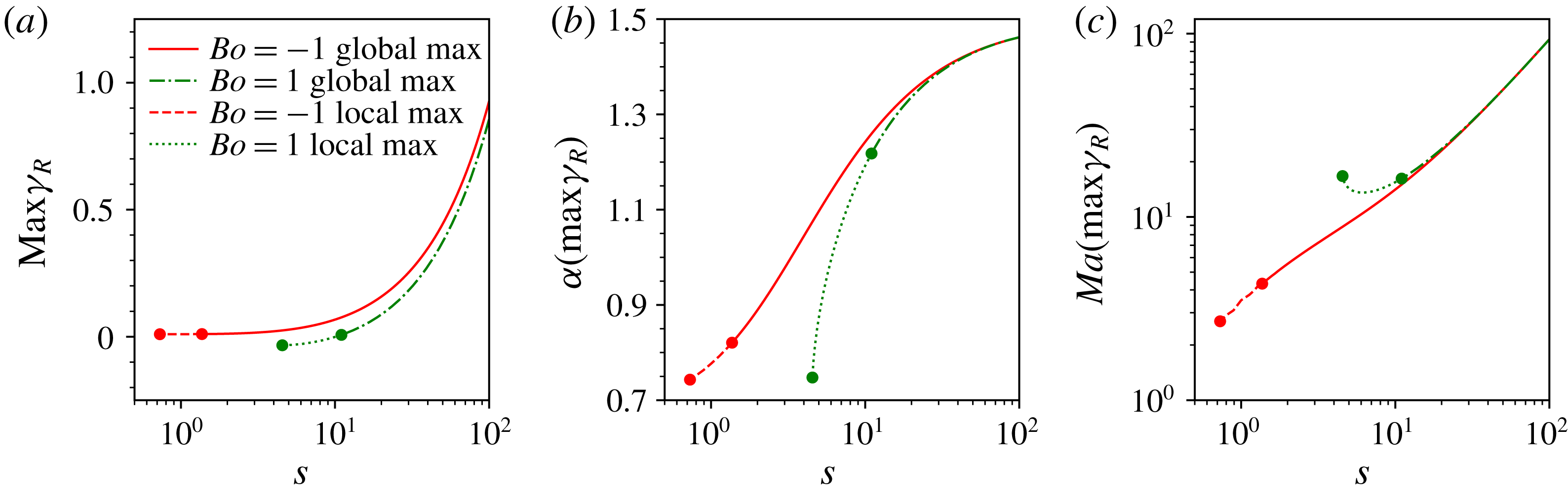
The influence of $s$ on (a) the maximum of $\unicode[STIX]{x1D6FE}_{R}$ over all $\unicode[STIX]{x1D6FC}$ and $Ma$ in the $Q$ sector (here at $n=2,\;m=5$ ) for two different values of $Bo$ , one positive and the other one negative. (b,c) The values of $\unicode[STIX]{x1D6FC}$ and $Ma$ at which this maximum occurs. The global maxima of $\unicode[STIX]{x1D6FE}_{R\,max}$ with respect to $Ma$ , present at larger $s$ , become local maxima between the pairs of dots on each curve. At smaller $s$ , to the left of the end dot on each curve, there are neither global nor local maxima.

Thus, we have observed here, for the first time, the existence of another route to the mid-wave instability: the continuous transition from long-wave instability (see the marked point $(Ma_{LM},0)$ in figure 2 f). Only the other route, the onset of mid-wave instability from stability, was present for the case of zero gravity (see HF). In the former scenario, the mid-wave instability has a non-zero growth rate and a finite support interval from the very beginning. A detailed investigation of the boundaries between the domains of the mid-wave instability, long-wave instability and stability in the $(Ma,Bo)$ -plane appears in § 5.

Figure 3 shows the dependencies of $\max \unicode[STIX]{x1D6FE}_{R}$ , defined as the maximum of $\unicode[STIX]{x1D6FE}_{R}$ over all $\unicode[STIX]{x1D6FC}$ and $Ma$ , along with the corresponding values of $\unicode[STIX]{x1D6FC}$ and $Ma$ at which this maximum occurs, denoted $\unicode[STIX]{x1D6FC}(\max \unicode[STIX]{x1D6FE}_{R})$ and $Ma(\max \unicode[STIX]{x1D6FE}_{R})$ , on the shear parameter $s$ in the $Q$ sector, similar to those shown in figure 13 of Part 1 for the other two sectors. We observe that the existence of the global maximum in $Ma$ of the growth rate maxima with respect to the wavenumber is less common in the $Q$ sector, especially for $Bo>0$ . At smaller values of $s$ , the global maximum becomes a local one like the one in figure 2(a). This is indicated in figure 3 as the change from the solid to the dashed curve for $Bo=-1$ and from the dashed to the dotted curve for $Bo=1$ . At still smaller $s$ , to the left of the end dot on each curve, there are neither global nor local maxima.

5 Stability diagrams of $(Ma,Bo)$ -plane

5.1 Regions of the long-wave and mid-wave instabilities

Here we present a detailed account of the mid-wave instability changes as the viscosity ratio is increased, starting from a value in the $R$ sector, $1<m<n^{2}$ , then crossing the $m=n^{2}$ border and further growing in the $Q$ sector, $m>n^{2}$ . In the $R$ sector, the robust branch is long-wave unstable provided $Bo<Bo_{cL}$ where $Bo_{cL}(Ma)$ ,

(5.1) $$\begin{eqnarray}Bo_{cL}=\frac{3\unicode[STIX]{x1D711}(m-n^{2})}{4n^{3}(1-m)(n+m)}Ma\end{eqnarray}$$

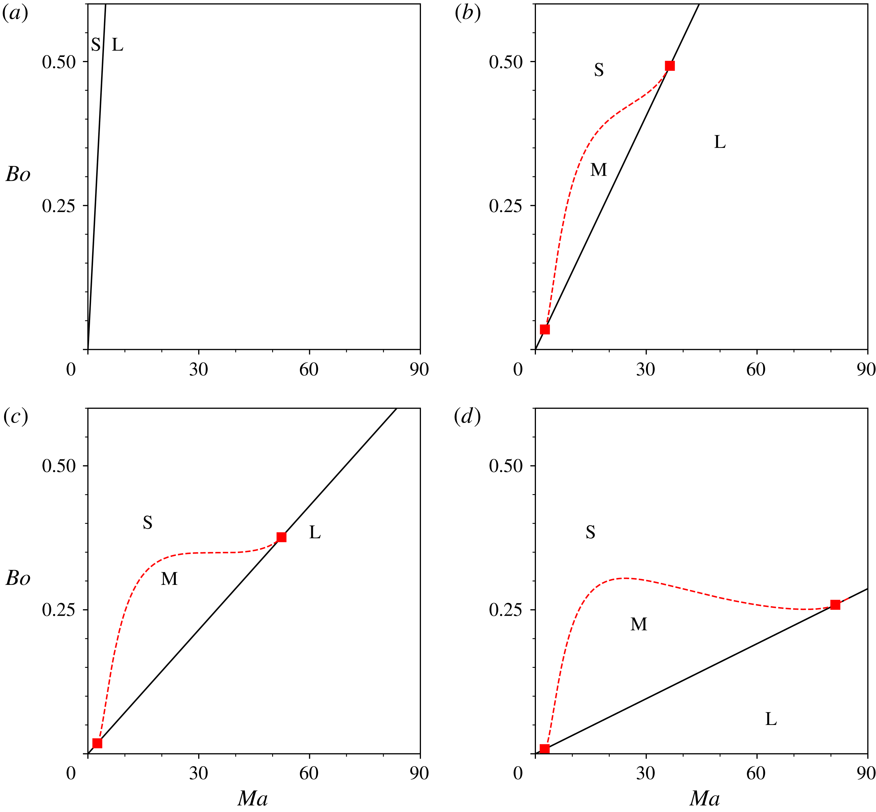
(see equation (4.36) of Part 1), is positive. If $m<n^{2}$ and sufficiently far from the $m=n^{2}$ border, there exists just one stability boundary, given by $Bo=Bo_{cL}$ ; it is a straight line (starting at the origin) that separates the long-wave unstable and stable regions, as shown in figure 4(a).

Figure 4.

Stability diagrams in the $(Ma,Bo)$ -plane showing the influence of the viscosity ratio $m$ as $m\uparrow n^{2}$ : (a) $m=10.25$ , (b)  $m=15$ , (c)  $m=15.45$ and (d)  $m=15.75$ . The solid and dashed curves represent long-wave and mid-wave instability boundaries respectively; S, L and M denote the stable, long-wave unstable and mid-wave unstable regions. Here $s=1$ and $n=4$ .

As $m$ increases and gets sufficiently close to $m=n^{2}$ , the onset of a mid-wave instability is observed for certain intervals of $Ma$ and $Bo$ . In figure 4(b,c), a mid-wave instability occurs provided $Bo_{cL}<Bo\,<Bo_{cM}$ , for a finite interval of the Marangoni numbers, $Ma_{LM1}<Ma<Ma_{LM2}$ , as the $Bo_{cL}$ and $Bo_{cM}$ curves ‘intersect’ each other at $Ma=Ma_{LM1}$ and $Ma=~Ma_{LM2}$ . 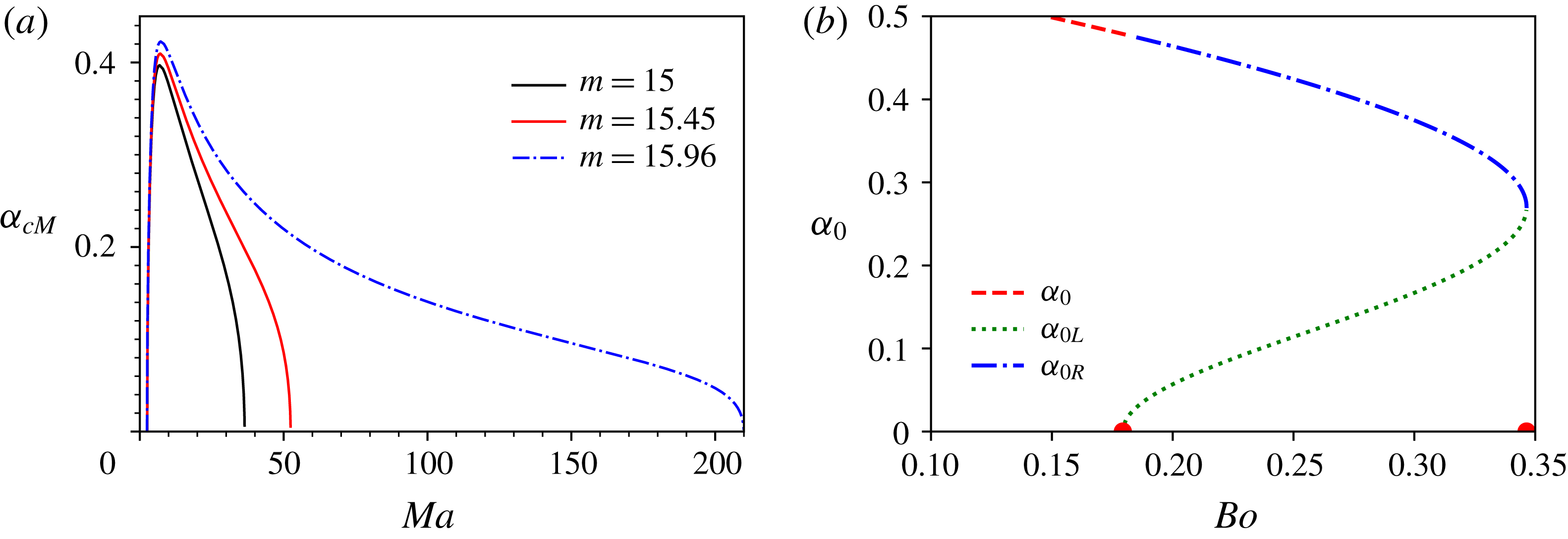The ‘quasi-intersection’ points, marked in the figure as filled squares, are the boundary points for the critical curve but are not the critical points themselves: the critical wavenumber decreases to zero as $Ma\rightarrow Ma_{LMj}$ , but the zero value is prohibited for a critical wavenumber. When $m$ is approaching ever closer to $n^{2}$ , at some $m$ the critical curve of the mid-wave instability acquires a maximum and a minimum, such as the ones in figure 4(d). Clearly, for each fixed $Ma$ of the $Ma$ interval $Ma_{LM1}<Ma<Ma_{LM2}$ , there are three distinct $Bo$ intervals: a semi-infinite interval of stability $Bo>Bo_{cM}$ ; a finite interval of mid-wave instability $Bo_{cL}<Bo<Bo_{cM}$ ; and a semi-finite interval of long-wave instability $Bo<Bo_{cL}$ .

In figure 5(a), the wavenumber $\unicode[STIX]{x1D6FC}_{cM}$ corresponding to $Bo_{cM}$ is plotted versus $Ma$ for the values of $m$ corresponding to figure 4(b,c) and also for $m=15.96$ , which is closer to the $m=n^{2}$ boundary value, $m=16$ , than $m=15.75$ of figure 4(d). With this, figure 5(a) suggests the hypothesis that in approaching the sector boundary, the larger quasi-intersection value of $Ma$ tends to infinity. The latter is in accordance with the stability diagram for the sector boundary value $m=16$ (see figure 6).

Figure 5.

(a) The critical wavenumber $\unicode[STIX]{x1D6FC}_{cM}$ versus Marangoni number $Ma$ for the same parameter value choices as in figure 4, except for the largest value of $m$ being $m=15.96$ . (b) The marginal wavenumbers $\unicode[STIX]{x1D6FC}_{0}$ , $\unicode[STIX]{x1D6FC}_{0L}$ and $\unicode[STIX]{x1D6FC}_{0R}$ versus Bond number $Bo$ for $s=1$ , $Ma=25$ , $n=4$ and $m=15.45$ . There is mid-wave instability in the $Bo$ region bounded by the two semicircles on the horizontal axis, long-wave instability to the left of this region and stability to the right of this region.

For all these cases, $\unicode[STIX]{x1D6FC}_{cM}$ attains a maximum at $Ma$ such that $Ma_{LM1}<Ma<Ma_{LM2}$ . Figure 5(b) shows, for the parameters of figure 4(c) and $Ma=25$ , that, as the Bond number grows, when it reaches the value $Bo_{cL}$ , the long-wave instability changes into the mid-wave one by the left endpoint of the interval of unstable $\unicode[STIX]{x1D6FC}$ departing from the zero $\unicode[STIX]{x1D6FC}$ point.

The unstable $\unicode[STIX]{x1D6FC}$ interval continues to shrink from both ends, and finally becomes a single non-zero $\unicode[STIX]{x1D6FC}$ point at $Bo=Bo_{cM},$ the rightmost point of the curve. The maximum growth rate (not shown) decreases to zero at this point, and there is stability for larger $Bo$ , in agreement with figure 4(c).

Figure 6.

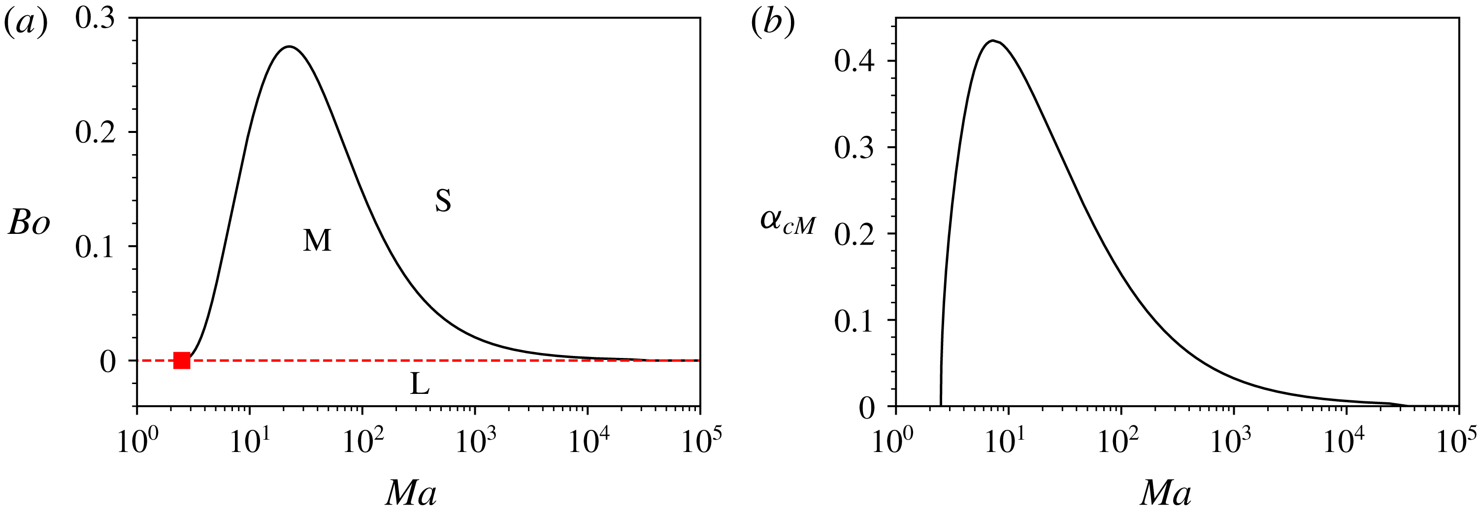
(a) Stability diagram in the ( $Ma,Bo$ )-plane similar to the ones shown in figure 4, for a case where $m=n^{2}$ (here $m=16$ ) and (b) the corresponding critical wavenumber, $\unicode[STIX]{x1D6FC}_{cM}$ . The end points have $Ma=5/2$ . Here $s=1$ .

On the $m=n^{2}$ border (e.g. for $m=16$ and $n=4$ ), the robust branch is long-wave unstable in the half-plane $Bo<0$ (with the boundary line $Bo_{cL}=0$ ), as shown in figure 6. Along the $Ma$ -axis ( $Bo=0$ ), the stability results of HF that show the existence of a mid-wave instability for $Ma>5/2$ are recovered: $Ma_{LM1}=5/2$ and $Ma_{LM2}=\infty$ . Notably, $Bo_{cL}(Ma)\downarrow 0$ as $Ma\rightarrow \infty$ . We also note that there is just a single extremum, a maximum, on the critical curve.

Figure 7.

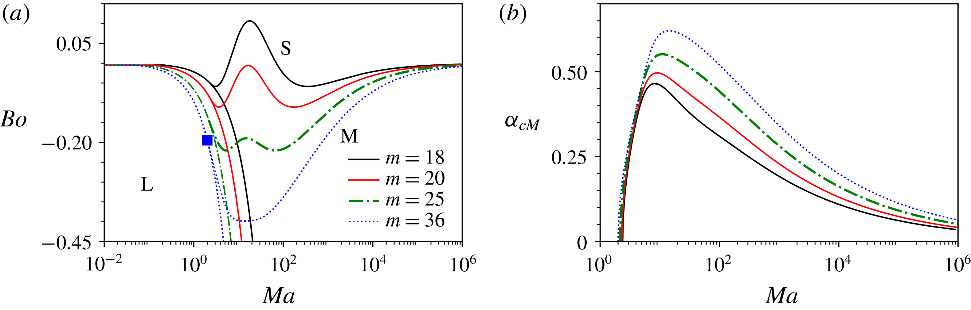
(a) Stability diagram showing the regions of mid-wave and long-wave instability and stability defined by the curves $Ma_{cL}$ and $Ma_{cM}$ as $m$ increases in the $Q$ sector, and (b) the wavenumber corresponding to $Ma_{cM}$ for the indicated values of $m$ . Here $n=4$ and $s=1$ .

In the $Q$ sector, $Bo_{cL}(Ma)<0$ , as given by (5.1). The threshold curves $Bo=Bo_{cL}(Ma)$ are plotted in figure 7 for each value of $m$ represented there; all the threshold curves have the ( $Bo$ , $Ma$ )-origin as their left-hand end (with linear scales on both axes, all the threshold lines would start from the origin and have a negative slope). The long-wave instability occurs below each threshold curve; the region of long-wave instability is labelled with an ‘L’ in the figure. At some point on each L-threshold curve, the critical curve of the mid-wave instability begins, going unbounded rightward, in the direction of increasing $Ma$ ; as $Ma\uparrow \infty$ , each critical curve is asymptotic to $Bo=0$ (thus, different from the $R$ sector, but similar to the boundary between the $R$ and $Q$ sectors, the threshold line of the long-wave instability intersects the critical curve of the mid-wave instability at a single point); however, in contrast with the boundary between the $R$ and $Q$ sectors, the critical curve approaches the axis $Bo=0$ from below. Also, at the threshold-critical quasi-intersection, the $Bo_{cL}(Ma)$ increases as $Ma\downarrow Ma_{LM1}$ . Since there is still a local maximum on the critical curve, just as there is one in the $R$ sector and on the sector boundary $m=n^{2}$ , it follows that there must be at least two local minima as well.

The mid-wave instability occurs below such a critical curve $Bo=Bo_{cM}$ (and above, or to the right of, the right-hand part ( $Ma>Ma_{LM1}$ ) of the corresponding threshold curve $Bo=Bo_{cL}(Ma)$ ). This region is labelled with an ‘M’. Above the critical curve, as well as above the left-hand part ( $Ma<Ma_{LM1}$ ) of the corresponding threshold curve, the flow is stable. The critical curve is given by a single-valued function $Bo=Bo_{cM}(Ma)$ , that is seen in figure 7 to have two local minima and a maximum in between them, provided the viscosity ratio $m$ is below a certain value $m_{N}$ . These two minima appear to occur at the same value of $Bo$ , and as $m$ increases all three extrema move downward, but the single maximum moves faster than the two minima. Eventually, at $m=m_{N}$ , the three extrema merge into a single minimum, such as the one on the $m=36$ critical curve.

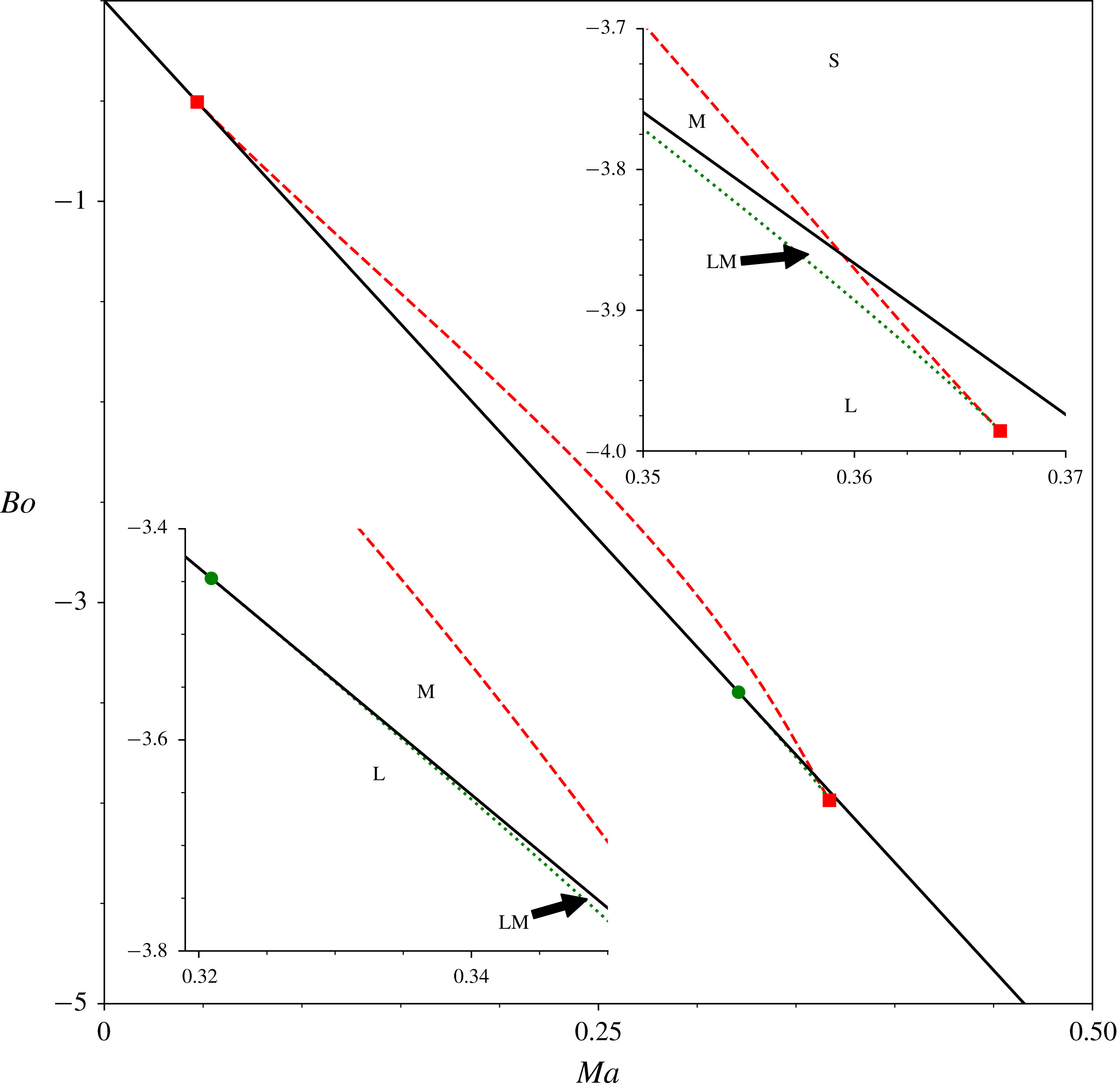
In the $S$ sector, as was mentioned at the end of section 5.2 of Part 1, the mid-wave instability occurs for the robust mode, although it is overshadowed by the long-wave instability of the surfactant mode. This is illustrated in figure 8 for the parameter values indicated there. The zoom-in, the upper inset, shows that, in contrast with the other sectors, the critical curve does not end at its intersection with the threshold curve of the linear instability, but continues below the intersection, until it meets another critical curve. On the latter curve, each point corresponds to a dispersion curve having zero growth rate at a local minimum (as illustrated in figure 9). The lower inset of figure 8 is a zoom-in near the quasi-intersection point of the lower critical curve and the threshold line, marked by a small circle, located at $Ma$ slightly above 0.32 and $Bo$ slightly above $-3.45$ . The quasi-intersection point of the upper critical curve and the threshold line, marked by a small square, is located at $Ma$ slightly above 0.046 and $Bo$ slightly below $-0.5$ .

Figure 8.

(a) Stability diagram of the less unstable mode for $s=1$ , $n=10$ and $m=0.1$ . The long-wave instability is present below the solid line and absent above it, while the mid-wave instability is present between the dashed curve, and either the solid line or the dotted curve. The upper and lower insets zoom in on the regions near the two lower pairwise intersections, marked by the square and the circle, respectively.

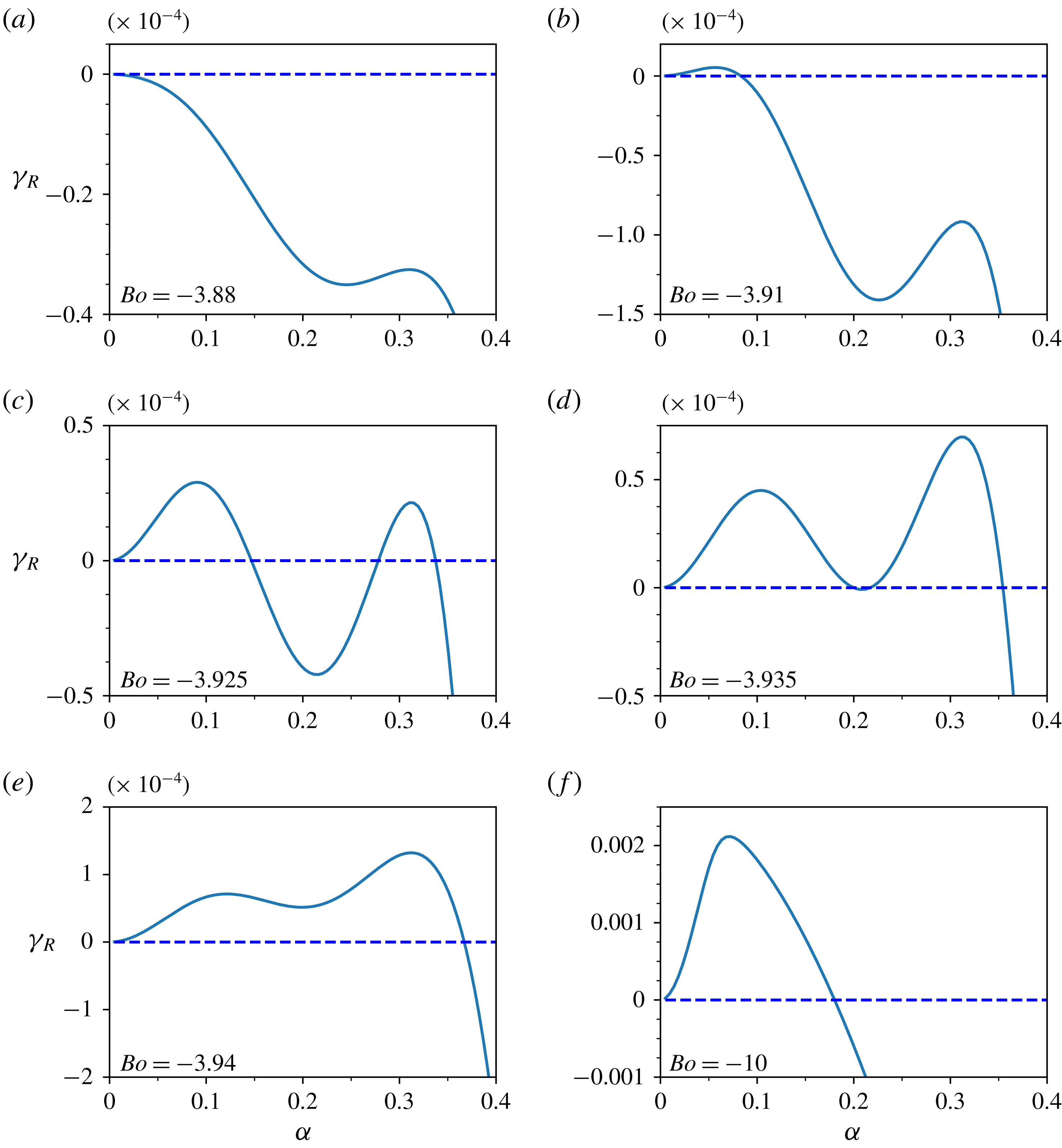
Figure 9 illustrates the change of the dispersion curves of the robust mode for the same values of $n$ , $m$ and $s$ as in figure 8, and $Ma$ fixed at 0.363 for a decreasing sequence of $Bo$ values corresponding to moving in the upper inset of figure 8 from the domain of stability (figure 9 a) to long-wave instability (figure 9 b) to the domain of coexisting long-wave and mid-wave instabilities (figure 9 c) to the lower critical curve (corresponding to the zero minimum in figure 9 d) and finally to the domain of long-wave instability (see figure 9 e,f). The mid-wave instability starts at a certain $Bo$ between those of figure 9(b,c) as the maximum, which is negative in figure 9(b), grows through the zero to positive values as in figure 9(c) near $\unicode[STIX]{x1D6FC}=0.3$ . In this process both intervals of (coexisting) long-wave instability and mid-wave instability expand, until they coalesce which corresponds to the snapshot shown in figure 9(d). Also, in going from figure 9(c) to figure 9(d), the local minimum increases from negative to zero value, and becomes positive, as in figure 9(e). Finally, this minimum disappears, and the dispersion curve has a single maximum (see figure 9 f).

Figure 9.

Dispersion curves for the robust mode in the $S$ sector. Here $n=10$ , $m=0.1$ , $s=1$ and $Ma=0.363$ . The values of $Bo$ are as indicated in each panel.

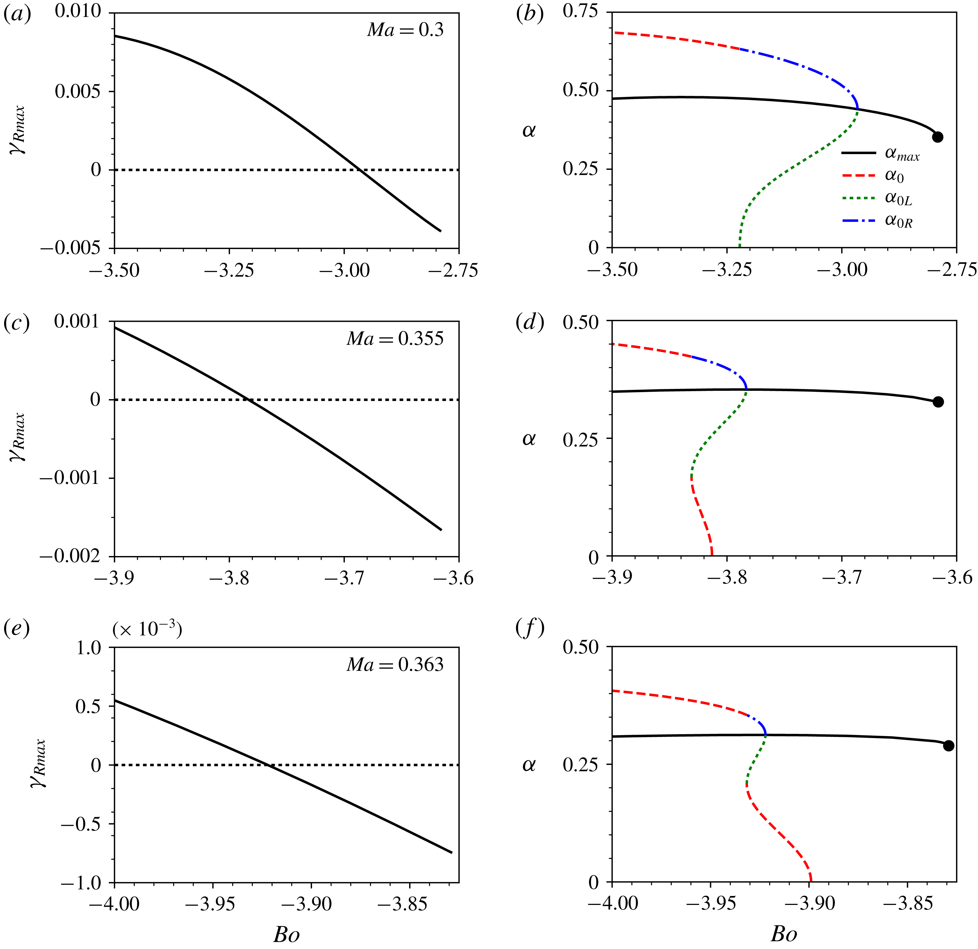
Figure 10 shows the salient features of the dispersion curves, such as the maximum growth rate, $\unicode[STIX]{x1D6FE}_{R\,max}$ , the corresponding wavenumber, $\unicode[STIX]{x1D6FC}_{max}$ , and the marginal wavenumbers, $\unicode[STIX]{x1D6FC}_{0}$ , $\unicode[STIX]{x1D6FC}_{0L}$ and $\unicode[STIX]{x1D6FC}_{0R}$ , as continuous functions of the Bond number for three different values of the Marangoni number. In particular, figure 9 corresponds to figure 10(e,f). For smaller values of the Marangoni number, such as $Ma=0.355$ in figure 10(c,d), which are to the left of the intersection of the (maximum) critical curve and the threshold curve, the mid-wave instability emerges before the long-wave instability as the value of $Bo$ becomes more negative (see the upper inset of figure 8). For a small range of $Bo$ , both long-wave and mid-wave instabilities can coexist (indicated by the label ‘LM’ in the upper inset of figure 8). This stage is followed by a completely long-wave unstable regime. For still smaller $Ma$ , such as $Ma=0.3$ , in figure 10(a,b), we observe the emergence of the mid-wave instability, which, subsequently, turns into a long-wave instability, similar to figure 5(b).

Figure 10.

Plots of $\unicode[STIX]{x1D6FE}_{R\,max}$ , the corresponding $\unicode[STIX]{x1D6FC}_{max}$ and the marginal wavenumbers $\unicode[STIX]{x1D6FC}_{0}$ , $\unicode[STIX]{x1D6FC}_{0L}$ and $\unicode[STIX]{x1D6FC}_{0R}$ versus $Bo$ in the $S$ sector for the indicated values of $Ma$ . Here $n=10$ , $m=0.1$ and $s=1$ . Note that when there are two local maxima on the dispersion curves, $\unicode[STIX]{x1D6FE}_{R\,max}$ shown here corresponds to the right-hand maximum even if it is smaller than the left-hand one.

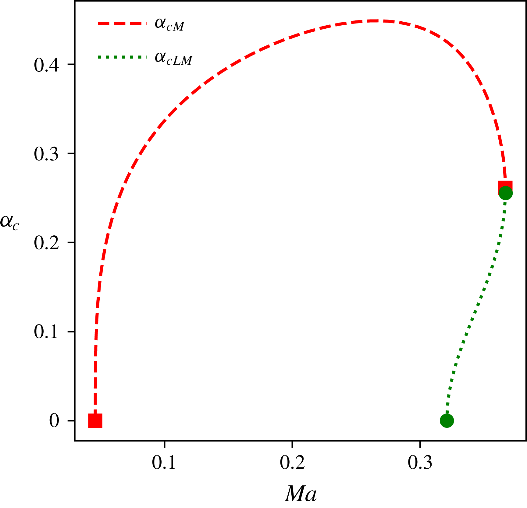
Figure 11 shows a plot of the critical wavenumber corresponding to the two critical curves in figure 8. It shows, similar to the analogous figures for the other two sectors, that the critical wavenumber, $\unicode[STIX]{x1D6FC}_{c}$ , approaches zero at the quasi-intersection points. It also reveals that the rate of change of the critical wavenumber approaches infinity at the common point of the two critical curves. Using small wavenumber expansions as described in § 5.2, we obtained the cubic equation given by (5.13) below, and solved it numerically to verify that at the left quasi-intersection point $Ma=0.0458$ , and at the other one $Ma=0.321$ .

Figure 11.

Critical $\unicode[STIX]{x1D6FC}$ versus $Ma$ corresponding to figure 8.

5.2 Asymptotics of the critical curves near their boundaries

5.2.1 General considerations

It should be possible to establish the asymptotic behaviour of the critical curves near their boundaries, in particular the sense of the curve inclination at a finite boundary point, a priori, using only minimal numerical information. This, as already indicated above, leads to certain conclusions about the number and sense of possible extrema, that in their turn facilitate the complete determination of the curve extrema. Near any finite quasi-intersection point, for both $R$ and $Q$ sectors, we look for the critical point coordinates in the form of generic power expansions

(5.2) $$\begin{eqnarray}Ma=Ma_{0}+\unicode[STIX]{x1D6FC}^{2}Ma_{2}+\unicode[STIX]{x1D6FC}^{4}Ma_{4}+\cdots\end{eqnarray}$$

and

(5.3) $$\begin{eqnarray}Bo=Bo_{0}+\unicode[STIX]{x1D6FC}^{2}Bo_{2}+\unicode[STIX]{x1D6FC}^{4}Bo_{4}+\cdots \,,\end{eqnarray}$$

where, to simplify notations, $Ma_{0}$ stands for $Ma_{LMj}$ (with $j=1,2$ ), etc. We substitute these expansions into the critical curve (4.1) and (4.2) and require the collected coefficients of each power to vanish. Since the point ( $Ma_{0}$ , $Bo_{0}$ ) lies on the threshold curve of the long-wave instability, we have $Bo_{0}=\unicode[STIX]{x1D705}Ma_{0}$ , where $\unicode[STIX]{x1D705}$ is the coefficient of $Ma$ in (5.1). Because of this relation, the leading orders $\unicode[STIX]{x1D6FC}^{6}$ in (4.1) and $\unicode[STIX]{x1D6FC}^{5}$ in (4.2) are satisfied identically. The next order system, given by the orders $\unicode[STIX]{x1D6FC}^{8}$ in (4.1) and $\unicode[STIX]{x1D6FC}^{7}$ in (4.2), is

(5.4) $$\begin{eqnarray}\displaystyle & \displaystyle k_{206}Ma_{2}+k_{116}Bo_{2}=r_{1}, & \displaystyle\end{eqnarray}$$

(5.5) $$\begin{eqnarray}\displaystyle & \displaystyle 6k_{206}Ma_{2}+6k_{116}Bo_{2}=8r_{1}, & \displaystyle\end{eqnarray}$$

where $k_{206}$ and $k_{116}$ are the leading-order coefficients such that $k_{20}\approx k_{206}\unicode[STIX]{x1D6FC}^{6}$ and $k_{11}\approx k_{116}\unicode[STIX]{x1D6FC}^{6}.$ In terms of the system parameters,

(5.6) $$\begin{eqnarray}\left.\begin{array}{@{}c@{}}\displaystyle k_{206}=\frac{n^{4}}{108}\unicode[STIX]{x1D711}(n-1)(n+1)^{2}(m-n^{2})s^{2},\\ \displaystyle k_{116}=\frac{n^{7}}{81}(n-1)(n+1)^{2}(m-1)(n+m)s^{2}.\end{array}\right\}\end{eqnarray}$$

On the right-hand sides of (5.4) and (5.5), $r_{1}$ is a cubic polynomial in $Ma_{0}$ whose coefficients are known combinations of $k_{pqr}$ (the coefficients of $\unicode[STIX]{x1D6FC}^{r}$ in the expansions of $k_{pq}$ ), and which lacks the quadratic term (cf. the discussion around (5.19)). The consistency of this system requires that $r_{1}=0$ , which is a cubic equation for $Ma_{0}$ . Clearly $Bo_{2}=-(k_{206}/k_{116})Ma_{2}$ , which simplifies to

(5.7) $$\begin{eqnarray}Bo_{2}=\unicode[STIX]{x1D705}Ma_{2}.\end{eqnarray}$$

The cubic equation for $Ma_{0}$ can be examined using the well-known Cardano formula and the underlying theory for the case with real coefficients.

The inclination of a critical curve at any quasi-intersection point is

(5.8) $$\begin{eqnarray}\text{d}Bo/\text{d}Ma=(\text{d}Bo/\text{d}\unicode[STIX]{x1D6FC})/(\text{d}Ma/\text{d}\unicode[STIX]{x1D6FC}).\end{eqnarray}$$

Using (5.2) and (5.3) we get $\text{d}Bo/\text{d}Ma=Bo_{2}/Ma_{2}=\unicode[STIX]{x1D705}$ , where we have used (5.7). Thus, at the boundary point, the critical curve is tangent to the threshold curve through that quasi-intersection point.

5.2.2 The $R$ sector finite critical curves and the threshold for their existence

We find that in the $R$ sector the cubic equation for $Ma_{0}$ has two distinct positive roots, corresponding to the two quasi-intersection points, for $m$ greater than some threshold value $m_{d}$ , and one non-physical negative root. For $m=m_{d}$ , the two positive roots merge into a single double root, which means that the interval of mid-wave instability shrinks to a single point, so that there is no mid-wave instability for $m<m_{d}$ . If the cubic equation is written in the form $Ma_{0}^{3}+pMa_{0}+q=0$ , the condition for the double root is that a certain discriminant is zero, or $27q^{2}+4p^{3}=0$ , whose solution for given $n$ and $s$ is $m_{d}$ , the threshold value above which the mid-wave instability exists. For example, when $n=4$ and $s=1$ , as in figure 4, $m_{d}=10.2783$ . This value of $m$ is between those for figure 4(a,b), as it should be. Thus, one can predict also the location of the boundaries of the critical curves in the $R$ sector. A somewhat different way for this, leading to a cubic equation for $Bo$ , is as follows. A more explicit form of the system (4.1)–(4.2) is

(5.9) $$\begin{eqnarray}\displaystyle & \displaystyle C_{0}(Ma,\unicode[STIX]{x1D6FC},Bo)=Ma\left(A_{1}+A_{2}Ma+A_{3}Ma^{2}\right)=0, & \displaystyle\end{eqnarray}$$

(5.10) $$\begin{eqnarray}\displaystyle & \displaystyle \frac{\unicode[STIX]{x2202}C_{0}}{\unicode[STIX]{x2202}\unicode[STIX]{x1D6FC}}=Ma(A_{1}^{\prime }+A_{2}^{\prime }Ma+A_{3}^{\prime }Ma^{2})=0, & \displaystyle\end{eqnarray}$$

where

(5.11) $$\begin{eqnarray}A_{1}=k_{11}B+k_{13}B^{3},\quad A_{2}=k_{20}+k_{22}B^{2},\quad A_{3}=k_{31}B,\end{eqnarray}$$

and the prime stands for the $\unicode[STIX]{x1D6FC}$ -derivative. After dividing these equations by $Ma$ , the system consists of two quadratic equations, equations (5.9) and (5.10), from which we obtain two different linear equations for $Ma$ , one by eliminating the quadratic term, and the other by eliminating the zero-power term. The solvability condition, obtained by equating the two expressions for $Ma$ , is

(5.12) $$\begin{eqnarray}(A_{1}A_{3}^{\prime }-A_{1}^{\prime }A_{3})^{2}-(A_{1}A_{2}^{\prime }-A_{1}^{\prime }A_{2})(A_{2}A_{3}^{\prime }-A_{2}^{\prime }A_{3})=0.\end{eqnarray}$$

Since $\unicode[STIX]{x1D6FC}\downarrow 0$ near a boundary point, we use the small- $\unicode[STIX]{x1D6FC}$ expansions to find, to the leading order, the standard-form cubic equation

(5.13) $$\begin{eqnarray}Bo^{3}+p_{1}Bo+q_{1}=0,\end{eqnarray}$$

where the coefficients are

(5.14) $$\begin{eqnarray}p_{1}=k_{206}(k_{118}k_{206}-k_{116}k_{208})/g_{d}\end{eqnarray}$$

and

(5.15) $$\begin{eqnarray}q_{1}=k_{116}k_{206}^{2}/g_{d},\end{eqnarray}$$

with $g_{d}=k_{116}^{2}k_{318}-k_{116}k_{206}k_{228}+k_{206}^{2}k_{138}$ . Here $k_{118}$ is the coefficient of the $\unicode[STIX]{x1D6FC}^{8}$ correction in $k_{11}$ such that $k_{11}\approx k_{116}\unicode[STIX]{x1D6FC}^{6}+k_{118}\unicode[STIX]{x1D6FC}^{8}$ . In terms of the system parameters,

(5.16) $$\begin{eqnarray}k_{118}=\frac{s^{2}}{1215}(m-1)(n-1)n^{7}(n+1)^{2}(m(n(8n-3)+7)+n(n(7n-3)+8)).\end{eqnarray}$$

Similarly,

(5.17) $$\begin{eqnarray}k_{208}=\frac{1}{810}s^{2}(n-1)n^{4}(n+1)^{3}((m^{2}-n^{4})(3n^{2}+8n+3)-4m(n^{2}-1)n^{2}).\end{eqnarray}$$

The coefficients $k_{318}$ , $k_{228}$ and $k_{138}$ are all of the leading order $\unicode[STIX]{x1D6FC}^{8}$ . In terms of the system parameters,

(5.18a-c ) $$\begin{eqnarray}k_{318}=\frac{n^{6}}{324}(n^{3}+m)^{2},\quad k_{228}=\frac{n^{8}}{486}(n+m)(n^{3}+m),\quad k_{138}=\frac{n^{10}}{2916}(n+m)^{2}.\end{eqnarray}$$

(From these expressions, one can see, in particular, that both the numerator and denominator of $q_{1}$ are positive.) The viscosity value $m_{d}(n,s)$ satisfies the double-root condition

(5.19) $$\begin{eqnarray}27q_{1}^{2}+4p_{1}^{3}=0,\end{eqnarray}$$

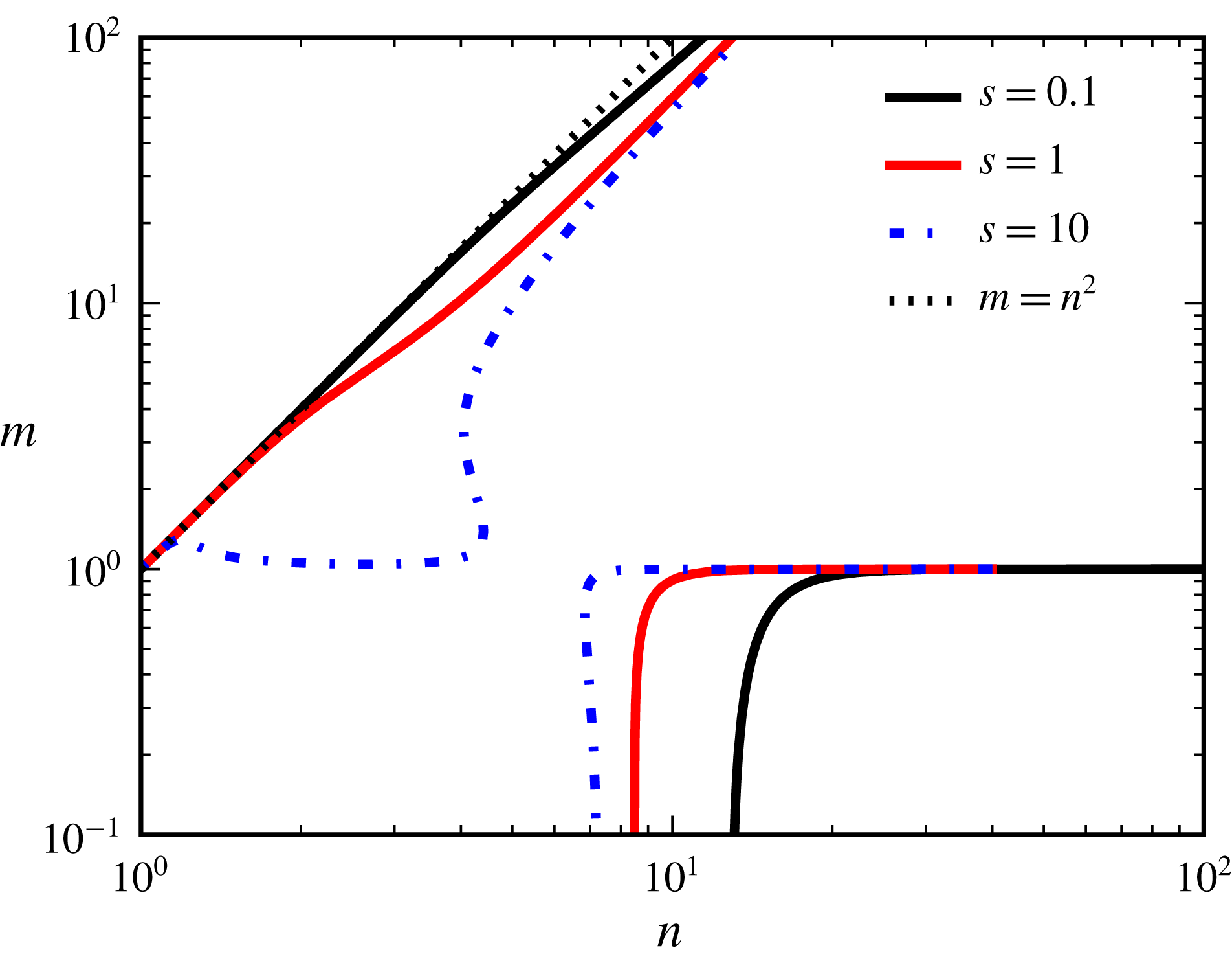
which is essentially the same equation as the one found above using a different approach, where no explicit expressions were shown for $p$ and $q$ (in fact, it is clear from relation (5.7) that $p_{1}=\unicode[STIX]{x1D705}^{2}p$ and $q_{1}=\unicode[STIX]{x1D705}^{3}q$ ). Fixing the value of $s$ , we solve numerically (5.19) for the solution curve $m=m_{d}(n)$ . In figure 12, we show these solution curves for several representative values of $s$ , ranging from small, to medium, to large. For large and small values of $s$ , numerical solutions can be verified with analytical asymptotics. It is difficult to get numerical solutions for very large $s$ . We find the asymptotics for $s\uparrow \infty$ in appendix C. In particular, we obtain the point ( $n=n_{0}$ , $m=1$ ) which is approached when $s\uparrow \infty$ by the $m_{d}$ curves of the $R$ and $S$ sectors (the upper and lower branches in figure 12).

Figure 12.

Numerical solutions of (5.19) for the representative values of $s$ given in the legend.

Consider now the asymptotic case $s\downarrow 0$ . Here, equation (5.19) simplifies to the leading-order equation $q_{1}=0$ , and thus its numerator is also zero. But this contradicts the fact, mentioned above, that it is strictly positive. Therefore, there is no mid-wave instability for sufficiently small base shear.

As was established in the last paragraph of § 5.2.1, at any boundary point of a critical curve, the latter is tangent to the threshold curve through that quasi-intersection point of the two curves. Hence, since in the $R$ sector the threshold curves have positive slopes (see figure 4), the same holds for the critical curves near their boundary points. This means that the critical function $Bo_{cM}(Ma)$ is increasing near its boundary points. Therefore, if there is a maximum, then there must be a minimum between this maximum and the right-end quasi-intersection point. It transpires that as $m$ rises through a certain threshold value $m_{t}$ , such a maximum and a minimum appear at some ( $Ma,Bo$ ). The latter is an inflection point on the $m=m_{t}$ critical curve, where the tangent is horizontal. We call it an ‘extrema bifurcation point’ (EBP; see figure 4 c). The EBPs, in both $Q$ and $R$ sectors, are discussed in detail in § 5.4.

5.2.3 The $Q$ sector semi-infinite critical curves and their asymptotic behaviour

Turning next to the $Q$ sector, the cubic equation for $Ma_{0}$ has a single positive root and two non-physical complex conjugate roots. The physical root corresponds to the single ‘quasi-intersection’ points in figure 7(a). Since the threshold curve has $Bo=Bo_{cL}(Ma)<0$ and for the critical curve $Bo\rightarrow 0$ as $Ma\rightarrow \infty$ , it is clear that the critical curve of the mid-wave instability lies above this threshold curve of the long-wave instability. This conclusion agrees with figure 7.

For the $Q$ sector, the fact of the shared direction with the threshold curve at the boundary point of the critical curve, $\text{d}Bo/\text{d}Ma=Bo_{2}/Ma_{2}=\unicode[STIX]{x1D705}$ (see the last paragraph of § 5.2.1), implies that the function $Bo_{cM}(Ma)$ is decreasing near the (single) quasi-intersection point. For $Ma\uparrow \infty$ , postulating, from numerical results, that $Bo\rightarrow 0$ and also $\unicode[STIX]{x1D6FC}\rightarrow 0$ , we look for asymptotics $Ma=c_{1}\unicode[STIX]{x1D6FC}^{-\unicode[STIX]{x1D701}}$ (with $c_{1}\neq 0$ ) and $Bo=d_{1}\unicode[STIX]{x1D6FC}^{\unicode[STIX]{x1D709}}$ (with $d_{1}\neq 0$ ), where $\unicode[STIX]{x1D701}$ and $\unicode[STIX]{x1D709}$ are positive. At leading order, the marginal wavenumber (4.1) (or, in more detail (3.9), which is convenient to divide by $Ma^{2}$ ) becomes

(5.20) $$\begin{eqnarray}k_{20}+k_{31}MaB=0.\end{eqnarray}$$

Since the $k_{20}\propto \unicode[STIX]{x1D6FC}^{6}$ , and $k_{31}\propto \unicode[STIX]{x1D6FC}^{8}$ , it follows that the product $MaB\propto \unicode[STIX]{x1D6FC}^{-2}$ . Since $B=Bo+\unicode[STIX]{x1D6FC}^{2}$ (which, clearly, entails that $\unicode[STIX]{x2202}B/\unicode[STIX]{x2202}\unicode[STIX]{x1D6FC}=0$ ), one can see that necessarily $\unicode[STIX]{x1D709}=2$ . This can be proved by showing that the assumption of $\unicode[STIX]{x1D709}<2$ or $\unicode[STIX]{x1D709}>2$ leads to a contradiction in the system consisting of (5.20) and

(5.21) $$\begin{eqnarray}k_{20}^{\prime }+k_{31}^{\prime }MaB+k_{31}Ma(2\unicode[STIX]{x1D6FC})=0\end{eqnarray}$$

(the partial derivative of (5.20) with respect to $\unicode[STIX]{x1D6FC}$ ).

Also it can be shown that $\unicode[STIX]{x1D709}=2$ implies $\unicode[STIX]{x1D701}=4$ . The omitted justification of these statements appears in Frenkel et al. (Reference Frenkel, Halpern and Schweiger2018). The system for $c_{1}$ and $d_{1}$ is now

(5.22a,b ) $$\begin{eqnarray}k_{206}+k_{318}(1+d_{1})c_{1}=0\quad \text{and}\quad 3k_{206}+k_{318}(5+4d_{1})c_{1}=0.\end{eqnarray}$$

Eliminating $k_{206}$ from the last two equations yields $d_{1}=-2$ . Then

(5.23) $$\begin{eqnarray}c_{1}=\frac{k_{206}}{k_{318}}=\frac{3(n-1)(m-n^{2})(n+1)^{2}}{n^{2}(n^{3}+m)^{2}}>0.\end{eqnarray}$$

Therefore, $Bo=c_{1}^{1/2}d_{1}Ma^{-1/2}<0$ . This is in excellent quantitative agreement with the numerical results documented in figure 7(a).

5.3 Local extrema of the critical curves

As figure 7 shows, in the $Q$ sector there is a local maximum on the critical curve for $m$ sufficiently close to $n^{2}$ , just as there is one at $m=n^{2}$ , the boundary between the $Q$ and $R$ sectors (see figure 6). Taking into account that $Bo_{cM}(Ma)$ is increasing at large $Ma$ (as it is negative and goes up to zero in the limit of infinitely increasing $Ma$ ), we conclude that there must be at least two local minima on the critical curve, which is also in agreement with the numerical results shown in figure 7(a). For sufficiently large $m$ , however, the critical curve is seen numerically to have just a single minimum.

At any extremum, be it in the $R$ or the $Q$ sectors, we have

(5.24) $$\begin{eqnarray}\frac{\text{d}Bo}{\text{d}Ma}=0.\end{eqnarray}$$

Also, since substituting the solutions $Bo(Ma)$ and $\unicode[STIX]{x1D6FC}(Ma)$ of the system of (4.1) and (4.2) for the critical curve into the left-hand side of (4.1) makes it true for all $Ma$ , the total $Ma$ -derivative of $C_{0}(Ma,\unicode[STIX]{x1D6FC}(Ma),Bo(Ma))$ must be zero. Writing the latter in terms of partial derivatives of $C_{0}$ with respect to $Ma$ , $\unicode[STIX]{x1D6FC}$ and $Bo$ , we use (5.24) and (4.2) to establish that $\unicode[STIX]{x2202}C_{0}/\unicode[STIX]{x2202}Ma=0$ . This is used as the third equation of the system for the extrema points, in addition to (4.1) and (4.2). Thus, using the explicit forms (5.9) and (5.10), we have the system of three quadratic equations

(5.25) $$\begin{eqnarray}\displaystyle & \displaystyle A_{1}+A_{2}Ma+A_{3}Ma^{2}=0, & \displaystyle\end{eqnarray}$$

(5.26) $$\begin{eqnarray}\displaystyle & \displaystyle A_{1}^{\prime }+A_{2}^{\prime }Ma+A_{3}^{\prime }Ma^{2}=0, & \displaystyle\end{eqnarray}$$

(5.27) $$\begin{eqnarray}\displaystyle & \displaystyle A_{1}+2A_{2}Ma+3A_{3}Ma^{2}=0, & \displaystyle\end{eqnarray}$$

where the last equation is the derivative of (5.9) with respect to $Ma$ . Subtracting (5.25) from (5.27), we get the linear equation

(5.28) $$\begin{eqnarray}A_{2}+2A_{3}Ma=0,\end{eqnarray}$$

which can be solved for $Ma$ in terms of the other variables, provided that $A_{3}\neq 0$ , i.e. since $k_{31}>0$ , that $B\neq 0$ . On the other hand, another linear equation for $Ma$ is obtained by eliminating the quadratic terms by linearly combining the quadratic (5.25) and (5.27):

(5.29) $$\begin{eqnarray}2A_{1}+A_{2}Ma=0.\end{eqnarray}$$

This can also be solved for $Ma$ in terms of the other variables (provided that $A_{2}\neq 0$ ; also, it is easy to see that one has to assume that $B\neq 0$ in order to have a non-zero $Ma$ ). The solvability condition of the over-determined system of the two linear equations for $Ma$ , equations (5.28) and (5.29), is

(5.30) $$\begin{eqnarray}\displaystyle {\mathcal{D}}:=A_{2}^{2}-4A_{1}A_{3}=0. & & \displaystyle\end{eqnarray}$$

Note that ${\mathcal{D}}=A_{2}^{2}-4A_{1}A_{3}$ is independent of $Ma$ .

One has to distinguish the cases $B\neq 0$ and $B=0$ . For $B\neq 0$ , the solution of (5.28) is

(5.31) $$\begin{eqnarray}Ma=-\frac{A_{2}}{2A_{3}}.\end{eqnarray}$$

Substituting this into the quadratic equation (5.26), we have a system of two transcendental equations for $B$ and $\unicode[STIX]{x1D6FC}$ , which can be written in the following form:

(5.32a,b ) $$\begin{eqnarray}{\mathcal{D}}=0\quad \text{and}\quad {\mathcal{D}}^{\prime }=0.\end{eqnarray}$$

In the $R$ sector, two solutions, a maximum and a minimum, are found by solving numerically the system of equations (5.32), and then finding $Ma$ from (5.31). In the $Q$ sector, this gives a single solution, which is a maximum for $m<m_{N}$ , and a minimum for $m>m_{N}$ .

Also, there are, in a certain interval of viscosity ratios, solutions with $B=0$ . In this case, the solvability condition (5.30) implies

(5.33) $$\begin{eqnarray}k_{20}=0,\end{eqnarray}$$

which yields the wavenumber. Then the Bond number is determined uniquely as

(5.34) $$\begin{eqnarray}Bo=-\unicode[STIX]{x1D6FC}^{2}.\end{eqnarray}$$

The quadratic equation (5.26), with the now known $\unicode[STIX]{x1D6FC}$ and $Bo$ , gives two distinct solutions for the Marangoni number if the discriminant $\unicode[STIX]{x1D701}$ is positive, where

(5.35) $$\begin{eqnarray}\unicode[STIX]{x1D701}=A_{2}^{^{\prime }2}-4A_{1}^{\prime }A_{3}^{\prime }.\end{eqnarray}$$

For the case at hand we have the simplified relations $A_{2}^{\prime }=k_{20}^{\prime }$ , $A_{1}^{\prime }=2\unicode[STIX]{x1D6FC}k_{11}$ and $A_{3}^{\prime }=2\unicode[STIX]{x1D6FC}k_{31}$ . Thus, the solutions are

(5.36) $$\begin{eqnarray}Ma=\frac{-k_{20}^{\prime }\pm \sqrt{k_{20}^{\prime 2}-16\unicode[STIX]{x1D6FC}^{2}k_{11}k_{31}}}{4k_{31}\unicode[STIX]{x1D6FC}},\end{eqnarray}$$

corresponding to the two minima on the critical curves in the $Q$ sector (see figure 7).

Figure 13.

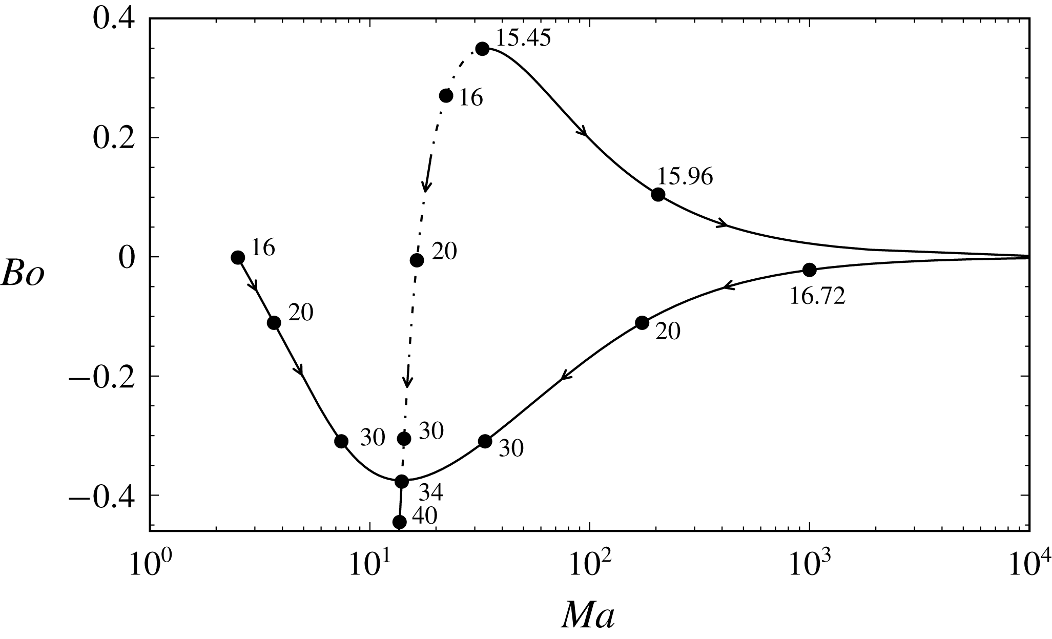
The trajectories of the extrema of the critical curves $Ma=Ma_{cM}(Bo)$ in the ( $Ma$ , $Bo$ )-plane (for $n=4$ and $s=1$ ; see figures 4 c,d, 6 a and 7 a) as $m$ changes starting in the $R$ sector and increasing through the $R$ sector and after that, for $m>16$ , the $Q$ sector. In the $R$ sector, for $15.45<m<16$ , there is one maximum, the dashed curve, and one minimum, the solid curve; for $16<m<34.31$ , there is one maximum between two minima; and finally, for $m>34.31$ , there is one minimum. The arrows indicate the increase of $m$ and the dots correspond to the displayed values of $m$ next to them. The minimum moves to infinite $Ma$ as $m\rightarrow 16$ , from either side.

Figure 13 shows the trajectories of the extrema in the $(Ma,Bo)$ -plane for $n=4$ as the viscosity ratio $m$ increases, starting from $m=15.45$ , in the $R$ sector, reaching the $Q$ sector at $m=16$ , and continuing to increase in the $Q$ sector. Consistent with the stability diagrams shown in figures 4 and 6, there are two extrema, a maximum and a minimum, for $m<16$ , which is in the $R$ sector, provided $m>m_{t}=15.45$ . In the $Q$ sector, there are three extrema as long as $m<m_{N}$ . At $m=m_{N}$ , the three extrema, one of them a maximum and two of them minima, collapse together into a single minimum, which then persists through the $Q$ sector. (Recall that we term this point the EBP.)

In connection with the non-monotonic character of critical curves that have multiple local extrema, we note the following. In figure 2(e,f) (where $n=2$ ), we see that as $Ma$ increases, the long-wave instability gives way to stability at $Ma=Ma_{cL}$ , which persists up to $Ma=Ma_{cM}$ , at which point the mid-wave instability sets in, further persisting for all larger $Ma$ . For short, we symbolically describe this sequence of $Ma$ intervals with different stability types as L–S–M (where L indicates the long-wave instability, S denotes stability and M stands for the mid-wave instability). The same stability interval sequence is obtained from figure 7 (where $n=4$ ) if, for example, we fix $m=25$ and $Bo=-0.1$ , and go rightwards parallel to the $Ma$ -axis. However, different sequences occur for other sets of parameters. For example, at $m=20$ and $Bo=-0.05$ , we observe the sequence L–S–M–S–M; at $m=36$ and $Bo=-0.3$ , the sequence is L–M–S–M; and at $m=25$ and $Bo=-0.2$ , we have the longer sequence L–M–S–M–S–M. It appears that for any $Bo<0$ , any sequence starts with L and ends with M. In contrast, for positive $Bo$ , e.g. at $Bo=0.05$ and $m=18$ , we have a S–M–S sequence of $Ma$ intervals.

5.4 Extrema bifurcation points

5.4.1 The EBPs in the Q sector

We turn now to the problem of equations determining the EBPs. In this section, we consider those in the $Q$ sector, while those in the $R$ sector are examined in the following section.

Clearly, the bifurcation point of the two minima and one maximum at $m=m_{N}$ in the $Q$ sector, which has $B=0$ (inherited, by continuity, from the $B=0$ property of the two minima existing at the smaller $m$ ), must satisfy, in addition to (4.1), (4.2) and (5.27), the condition that the $Ma$ values of the two minima coalesce to a double root. It is clear from (5.36) that this means

(5.37) $$\begin{eqnarray}k_{20}^{\prime 2}-16\unicode[STIX]{x1D6FC}^{2}k_{11}k_{31}=0.\end{eqnarray}$$

As we already noted above, the latter corresponds to the discriminant (5.35) being zero, so that the two solutions of (5.26) for the two minima of $Ma$ merge into just a single one. For the EBPs in the $Q$ sector, it is convenient to use new variables $n_{1}=n-1$ and $m_{1}=(m-n^{2})/(n-1)$ so that the $Q$ sector corresponds to the entire first quadrant. For any given ( $n_{1},m_{1}$ ), as we already mentioned above, we can find the other properties of the EBP as follows: first, $\unicode[STIX]{x1D6FC}$ is determined by solving (5.33). 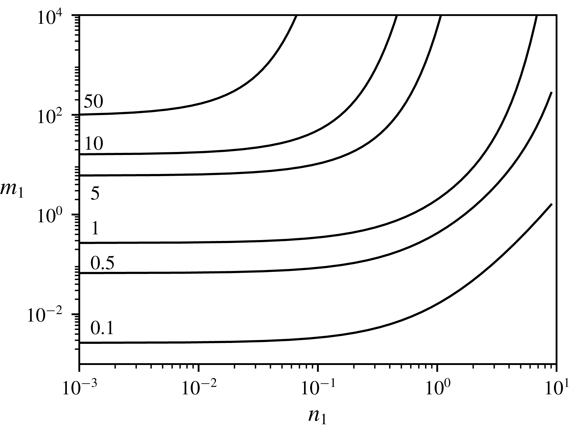This dependence $\unicode[STIX]{x1D6FC}(n_{1},m_{1})$ is shown as the contour plot in figure 14.

Figure 14.

Level curves of $\unicode[STIX]{x1D6FC}(n_{1},m_{1})$ for the EBPs in the $Q$ sector. The numbers next to the curves are the corresponding values of $\unicode[STIX]{x1D6FC}$ .

We observe this unique solution for the extended region of realistic $(n_{1},m_{1})$ . For small $n_{1}$ and $\unicode[STIX]{x1D6FC}$ , we find that asymptotically $m_{1}=(4/15)\unicode[STIX]{x1D6FC}^{2}$ , independent of $n_{1}$ , so that the level curves of $\unicode[STIX]{x1D6FC}$ intersect the vertical axis at different heights. With corrections, the equation of the level curves at $\unicode[STIX]{x1D6FC}\ll 1$ and $n_{1}\ll 1$ is $m_{1}=4/15\unicode[STIX]{x1D6FC}^{2}(1+5n_{1}/2+2n_{1}^{2})$ , where we have suppressed the terms which have powers of $\unicode[STIX]{x1D6FC}^{2}$ higher than one or powers of $n_{1}$ higher than two. Keeping the two correction terms in the formula is necessary for predicting the flip of the sign of the level curve curvature as one switches between the linear and log scales of the $n_{1}$ -axis.

Having found $\unicode[STIX]{x1D6FC}$ from (5.33), the Bond number $Bo(n_{1},m_{1})$ is given by (5.34) with $\unicode[STIX]{x1D6FC}=\unicode[STIX]{x1D6FC}(n_{1},m_{1})$ . Next, equation (5.37), after being divided through by $s^{2}$ , is a linear equation in $s^{2}$ , and gives $s(n_{1},m_{1})$ , provided the derivative of $k_{20}$ with respect to $\unicode[STIX]{x1D6FC}$ is negative. The argument showing this is the case, which involves some asymptotic dependencies, is omitted here but appears in Frenkel et al. (Reference Frenkel, Halpern and Schweiger2018)

Finally, $Ma(n_{1},m_{1})$ of the EBP is given by (5.36) with the discriminant equal to zero, so that

(5.38) $$\begin{eqnarray}Ma=\frac{-k_{20}^{\prime }}{4k_{31}\unicode[STIX]{x1D6FC}}.\end{eqnarray}$$

For example, there is a solution that corresponds to the EBP in figure 13, with $n=4$ , $s=1$ , $m=m_{N}=34.31$ , $Ma=13.97$ , $Bo=-0.375$ and $\unicode[STIX]{x1D6FC}=0.61$ . These values are also consistent with figure 7. Note that in figure 14  $\unicode[STIX]{x1D6FC}(n_{1},m_{1})$ has no external parameters. The same is true of the other EBP dependencies: $Bo(n_{1},m_{1})$ , $s(n_{1},m_{1})$ and $Ma(n_{1},m_{1})$ .

5.4.2 The EBPs in the $R$ sector

It was mentioned above, at the end of § 5.2.2, that one maximum and one minimum appear at the EBP on the critical curve in the $R$ sector corresponding to a threshold value $m_{t}$ of $m$ . It is clear that for this EBP

(5.39) $$\begin{eqnarray}\frac{\text{d}^{2}Bo}{\text{d}Ma^{2}}=0,\end{eqnarray}$$

where the implicit function $Bo(Ma)$ is given by the system (5.9) and (5.10). (This EBP corresponds to the inflection point with the horizontal tangent line in figure 4 c.) Using the implicit function differential formulas, we obtain a fourth equation of the system for the EBP:

(5.40) $$\begin{eqnarray}\displaystyle \left(\frac{\unicode[STIX]{x2202}^{2}C_{0}}{\unicode[STIX]{x2202}\unicode[STIX]{x1D6FC}\unicode[STIX]{x2202}Ma}\right)^{2}-\frac{\unicode[STIX]{x2202}^{2}C_{0}}{\unicode[STIX]{x2202}\unicode[STIX]{x1D6FC}^{2}}\frac{\unicode[STIX]{x2202}^{2}C_{0}}{\unicode[STIX]{x2202}Ma^{2}} & = & \displaystyle 2Ma(A_{2}+3A_{3}Ma)(A_{1}^{\prime \prime }+A_{2}^{\prime \prime }Ma+A_{3}^{\prime \prime }Ma^{2})\nonumber\\ \displaystyle & & \displaystyle -\,(A_{1}^{\prime }+2A_{2}^{\prime }Ma+3A_{3}^{\prime }Ma^{2})^{2}=0.\end{eqnarray}$$

(Some omitted intermediate details appear in Frenkel et al. (Reference Frenkel, Halpern and Schweiger2018).) We note that $Bo>0$ in the $R$ sector and therefore $B\neq 0$ . The four equations, given by (5.32), (5.31) and (5.40), are solved numerically. As an example, for $n=4$ and $s=1$ , we find $\unicode[STIX]{x1D6FC}=0.21$ , $Bo=0.35$ , $Ma=33.81$ and $m=m_{t}=15.45$ . These numbers are consistent with figure 4(c) and figure 13.

Similarly to the $Q$ sector procedure used above, for the four EBP equations in the $R$ sector, an algebraic reduction is possible where a single equation is used to solve for one variable, and then the three other parameters of the EBP are found (with given values of $n$ and $m$ ). For this, we note the algebraic identity $k_{22}^{2}-4k_{13}k_{31}=0$ which can be verified using the explicit expressions of $k_{22}$ , $k_{13}$ and $k_{31}$ in terms of $\unicode[STIX]{x1D6FC}$ and the system parameters (as given in Frenkel et al. (Reference Frenkel, Halpern and Schweiger2018)). Hence, the first and the second equations of (5.32) can be written, explicitly showing the $s$ and $B$ dependencies, as, respectively,

(5.41a,b ) $$\begin{eqnarray}k_{20s}^{2}s^{2}+2B^{2}k_{sB}=0\quad \text{and}\quad k_{20s}k_{20s}^{\prime }s^{2}+B^{2}k_{sB}^{\prime }+4B\unicode[STIX]{x1D6FC}k_{sB}=0.\end{eqnarray}$$

Here we have defined the quantity $k_{sB}$ as $k_{sB}=k_{20s}k_{22}-2k_{11s}k_{31}$ , where $k_{20s}$ and $k_{11s}$ are defined by $k_{20s}=k_{20}/s^{2}$ and $k_{11s}=k_{11}/s^{2}$ (so that they are independent of $s$ ). The last two displayed equations are linear equations for $s^{2}$ , so $s^{2}$ is obtained explicitly in terms of the quantities $\unicode[STIX]{x1D6FC}$ , $m$ , $n$ and $B$ . Moreover, the solvability condition of the over-determined system of the two linear equations for $s^{2}$ yields (after dividing through by $Bk_{20s}$ ) a linear equation for $B$ :

(5.42) $$\begin{eqnarray}B(k_{20s}k_{sB}^{\prime }-2k_{20s}^{\prime }k_{sB})+4k_{20s}\unicode[STIX]{x1D6FC}k_{sB}=0,\end{eqnarray}$$

whose coefficients depend on $\unicode[STIX]{x1D6FC}$ , $m$ and $n$ . Solving it (provided that the coefficient of $B$ is non-zero) yields $B$ in terms of $\unicode[STIX]{x1D6FC}$ , $m$ and $n$ ; using this expression in (5.41), we obtain $s^{2}$ in terms of $\unicode[STIX]{x1D6FC}$ , $m$ and $n$ , and then, from (5.31), an expression for $Ma$ in terms of $\unicode[STIX]{x1D6FC}$ , $m$ and $n$ . We substitute these expressions into (5.40) to obtain an equation containing $\unicode[STIX]{x1D6FC}$ , $m$ and $n$ , which can be numerically solved for $\unicode[STIX]{x1D6FC}$ giving it as a function of $n_{1}$ and $m_{1}$ . Then, for the given values of $n_{1}$ and $m_{1}$ , we find sequentially $B$ , $s^{2}$ and $Ma$ , in that order, using the linear-equations solutions for them described above. Thus, for given $n_{1}$ and $m_{1}$ , we determine all the parameters, $\unicode[STIX]{x1D6FC}$ , $B$ , $s$ and $Ma$ , of the corresponding EBP in the $R$ sector. The level curves of $\unicode[STIX]{x1D6FC}$ are seen in figure 15 as the monotonically rising curves. Through the upper point of each curve passes the level curve, with the same value of $\unicode[STIX]{x1D6FC}$ , of the $\unicode[STIX]{x1D6FC}$ function which makes identically vanish the coefficient $B_{d}$ of $B$ in (5.42). It is clear that the envelope of the family of level curves for $B_{d}=0$ is the locus of the upper ends of the level curves for the EBPs. (The envelope curve shown in the figure was obtained by solving the system $B_{d}=0$ and $\unicode[STIX]{x2202}B_{d}/\unicode[STIX]{x2202}\unicode[STIX]{x1D6FC}=0$ .) When approaching the envelope curve, the values of $B$ grow to infinity. The EBP level curves can be formally continued above the envelope curve, but lead to unphysical negative values of $B$ and $Ma$ . (Note that the $R$ sector is completely mapped into the region of the $(n_{1},-m_{1})$ -plane bounded above by the line $-m_{1}=n_{1}+2$ , corresponding to $m=1$ ; however, this line is outside the range of figure 15.)

Figure 15.

Level curves of $\unicode[STIX]{x1D6FC}(n_{1},\;m_{1})$ for the EBPs in the $R$ sector. (For other curves here, see the text.)

6 Summary and discussion

In Part 2 of our work, we considered the mid-wave regimes of linear instability, defined as those having a finite interval of unstable wavenumber bounded away from zero, for two immiscible Newtonian fluid layers flowing in a horizontal channel between parallel plates that move steadily with respect to each other driving a Couette flow. As in Part 1, we investigated, by using the normal modes for the linearized equations under conditions of negligible inertia, the joint effects of insoluble surfactants and gravity on the flow stability. Without any restrictions on the system parameters, such as the smallness of the thickness ratio (see e.g. Frenkel & Halpern (Reference Frenkel and Halpern2006) and Kalogirou & Papageorgiou (Reference Kalogirou and Papageorgiou2016), where nonlinear and/or inertial effects were included), the differential eigenvalue problem, involving the instability increment and the normal amplitudes, enjoys an analytical reduction to a low-dimensional algebraic eigenvalue problem, and then to a quadratic equation for the increment (unlike, for example, Picardo et al. (Reference Picardo, Radhakrishna and Pushpavanam2016), where the numerical solution of a full differential eigenvalue problem was necessary). The latter yields two continuous increment branches, and hence two continuous growth rate branches. As in FH and subsequent papers, one of the branches, that is present even when $Ma=0$ , is called the ‘robust’ branch, and the other one, that vanishes as $Ma\downarrow 0$ , is the ‘surfactant’ branch.

The mid-wave instability, the subject of Part 2, turns out to emerge in two distinct ways (as a control parameter increases): it starts either from a stability stage, which we call the true onset of the mid-wave instability, or, alternatively, from a long-wave instability stage. The latter occurs when the left endpoint of the interval of the unstable wavenumbers, which is zero for the long-wave instability, starts moving away from zero (as shown in figure 5 b), the maximum growth rate remaining positive all along. In the alternative scenario of the onset of the mid-wave instability, the maximum growth rate is equal to zero at a certain positive wavenumber, for which, therefore, the marginal wavenumber equation holds. But in view of the maximum, the partial derivative of the growth rate equals zero as well. Thus, we have a system of two equations, whose solution gives the critical values of the Marangoni number and the wavenumber as a function of the Bond number, for arbitrarily fixed values of the remaining three parameters. We follow, as the viscosity ratio is increased in the $R$ sector towards its boundary with the $Q$ sector, the emergence of the critical curve, and its consequent change, in the ( $Ma,Bo$ )-plane (figure 4). The critical curve has its two endpoints on the threshold curve of the long-wave instability. The latter is rightward-increasing in the $R$ sector, horizontal at the boundary with the $Q$ sector (figure 6) and a decreasing curve in the $Q$ sector (figure 7). The right-side endpoint of the critical curve moves away to infinity as we cross into the $Q$ sector. The critical wavenumber is small near a critical curve endpoint, and so one can look for the critical solutions in the form of asymptotic power series. This gives rise to a cubic equation for the endpoint locations. Analysis of this equation leads to conclusions which are in agreement with the numerical observations, such that the critical curve in the $R$ sector exists only above a certain value of the viscosity ratio and has two endpoints, while there is just one single endpoint in the $Q$ sector. In all cases, the critical curve at its endpoint is tangent to the long-wave threshold curve. We also obtain and solve equations for the extrema of the critical curve, obtaining conclusions that agree with the numerical results. In the $R$ sector, there is a certain value of the viscosity ratio below which the critical curve has no extrema, but above which it has exactly two extrema: a maximum and a minimum. The latter disappears into the right-side infinity at the boundary with the $Q$ sector, and so we have just one extremum at this boundary, a maximum. Moving into the $Q$ sector as the viscosity ratio increases, there are at first one maximum in between two minima on the critical curve. These extrema coalesce into a single minimum at a certain value of the viscosity ratio $m$ , and this minimum persists for the larger values of $m$ .

As we go from an arbitrary critical point to a critical extremum, one more constraint is added, which decreases the number of free parameters by one. The EBPs, at which the number of extrema changes, correspond to another reduction of the number of free parameters. Thus, for given $n$ and $m$ , they determine all the other values: the wavenumber; Marangoni number; Bond number; and the shear parameter of the corresponding EBP (figure 15). Thus, figures 1, 2, 7, 13 and 15 represent different levels of information about the stability properties. Namely, going from one of the figures to the next, in the given order, the description gets more refined. On the other hand, the amount of data in the description decreases, in a certain sense. Figure 1 gives the growth rates at every wavenumber, but all the parameters are fixed at certain values. So, out of the seven quantities, $\unicode[STIX]{x1D6FC}$ , $\unicode[STIX]{x1D6FE}_{R}$ , $Ma$ , $Bo$ , $m$ , $n$ and $s$ , six are independent variables, and just one quantity is a dependent variable. Thus, these data make up a six-dimensional hypersurface in the seven-dimensional space. Figure 2 corresponds to some five independent variables determining the values of the other two quantities, thus resulting in a five-dimensional manifold of data. Figure 7 corresponds to a four-dimensional manifold, figure 13 implies a three-dimensional manifold of data and figure 15 corresponds to a two-dimensional manifold parameterized by the independent variables $m$ and $n$ , whose values determine $\unicode[STIX]{x1D6FC}$ , $\unicode[STIX]{x1D6FE}_{R}$ , $Ma$ , $Bo$ and $s$ (where $\unicode[STIX]{x1D6FE}_{R}=0$ since our consideration here is confined to the critical conditions of mid-wave instability). The envelope curve in figure 15 corresponds to a one-dimensional curve in the seven-dimensional space of the relevant quantities. Finally, for the inflection point of the envelope curve in figure 15, there are no independent variables, and all seven quantities are uniquely determined.

There is the mid-wave instability of the robust branch in the $S$ sector too, albeit the long-wave instability of the surfactant branch is the stronger of the two there. In the $(Ma,Bo)$ -plane, in the vicinity of the threshold line of the long-wave instability, in addition to the more usual critical mid-wave curve which consists of the points that correspond to dispersion curves with zero maximum growth rate, there is, below the latter, another critical mid-wave curve, consisting of the points corresponding to dispersion curves with zero minimum growth rate (see figure 8). Correspondingly, as the Bond number decreases (to larger-magnitude negative values), it is possible that at some point after the onset of the mid-wave instability, the long-wave instability starts, whose wavenumber interval is initially small and does not intersect the mid-wave interval of unstable wavenumbers. The coexistence of the mid-wave and the long-wave instabilities lasts until their intervals coalesce, corresponding to the critical curve of zero minimum growth rates in the $(Ma,Bo)$ -plane. After this coalescence, there is just one long-wave continuous interval of the unstable wavenumbers, with the dispersion curve having two positive local maxima of the growth rate at first, but just one single maximum eventually, at the most negative Bond number values. For another range of Marangoni number, an alternative scenario is possible, which differs from the one described above solely in that the long-wave instability starts first and the mid-wave one at the smaller (more negative) values of the Bond number. The consequent coalescence into purely long-wave instability is the same in both scenarios (figures 9 and 10).