3.1 Numerical mass flow rate

Detailed information about the local flow characteristics inside the channel is important for the analysis of the average characteristic measurements, such as the mass flow rate; however, this was not easy to obtain experimentally. Therefore, we also employed a numerical simulation for further analysis.

Various authors have analysed stationary thermal creep flows through channels of rectangular cross-section or parallel plates by using the linearized kinetic models (BGK (Stvorik, Park & Loyalka Reference Stvorik, Park and Loyalka1978) and S-model (Sharipov Reference Sharipov1999; Graur & Ho Reference Graur and Ho2014)) or by solving the linearized Boltzmann equation (Ohwada, Sone & Aoki Reference Ohwada, Sone and Aoki1989; Sone Reference Sone2002). These approaches are indispensable in the transitional flow regime, where the continuum approach is no longer valid but the collisionless Boltzmann equation cannot be applied yet. In all these publications, it was assumed that the local pressure and temperature gradients along the channel

were small enough for the linearization of the kinetic equations. This assumption, (3.1), allows the presentation of the mass flow rate through a channel of rectangular cross-section in the linear form

In expressions (3.1) and (3.2), the $z$ -axis coincides with the direction of the temperature gradient and of the channel’s largest dimension (channel length $L$ ). The local dimensionless flow rates, $G_{p}$ and $G_{T}$ , are induced by the local gradients of pressure and temperature, (3.1), respectively, and they depend on the local rarefaction parameter ${\it\delta}$ and on the accommodation coefficient ${\it\alpha}$ . In the numerical simulation we assumed, unless stated otherwise, full accommodation, i.e. ${\it\alpha}=1$ , at walls in the frame of the Maxwell diffuse–specular kernel. It is important to note that $T$ and $p$ in (3.2) are respectively the temperature and pressure at a local point inside the channel.

Equation (3.2) was integrated numerically by using the property of mass conservation and the values of the dimensionless mass flow rates $G_{p}({\it\delta})$ and $G_{T}({\it\delta})$ , obtained in Graur & Ho (Reference Graur and Ho2014) for a channel with $W/H$ ratio equal to 0.0367, which corresponds to the real channel’s dimensions. The equality of the pressure in both inlet and outlet reservoirs was used as the boundary condition for the pressure. From this integration, the mass flow rate ${\dot{M}}$ was obtained together with the pressure distribution along the channel; see Sharipov (Reference Sharipov1999) and Graur & Ho (Reference Graur and Ho2014) for more details. To extract both these flow characteristics, a linear temperature distribution along the channel walls was assumed. In § 4.1, the numerical results will be compared with the measurements of mass flow rate.

3.2 Effect of pressure profiles inside the microchannel

The mass flow rate ${\dot{M}}$ expressed at a local point is, as mentioned above, known to be decomposed into two terms, as in (3.2). The first and second terms represent pressure- and temperature-driven flows, respectively. Even though the flow inside the microchannel at $t=0$ was largely dominated by the temperature-driven flow (Rojas-Cárdenas et al. Reference Rojas-Cárdenas, Graur, Perrier and Méolans2013), there would be a slight pressure gradient along the microchannel, which would induce a flow. The fraction of the total mass flow rate caused by the pressure gradient can be estimated from the first term of (3.2), i.e. the reduced flow rate induced by a pressure gradient. To obtain this information, (3.2) was integrated along the channel as follows:

To establish (3.3) from (3.2), the property of mass conservation was used. When integrating the first term in (3.3), we implemented the pressure distribution along the channel, obtained, as explained in § 3.1, from the numerical solution of (3.2). To integrate the second term in (3.3), a linear distribution of the temperature was assumed. After integration, the ratio of the pressure-driven mass flow rate $\dot{M_{p}}$ to the total mass flow rate ${\dot{M}}$ was calculated. It was found that the term $\dot{M_{p}}$ appeared to be less than 0.1 % of the total mass flow rate ${\dot{M}}$ for ${\rm\Delta}T=37~\text{K}$ and less than 0.2 % for ${\rm\Delta}T=58~\text{K}$ . These results indicate that the pressure profile along the microchannel is nearly flat, i.e. the pressure-driven flow is negligible at $t=0$ , when the mass flow rate is driven only by the temperature gradient.

3.3 Temperature-driven mass flow rate

Taking into account the previous results, obtained in § 3.2, on the part of the pressure-induced mass flow rate in the total mass flow rate, it is reasonable to approximate the total mass flow rate, (3.3), by just the temperature gradient term:

Since this expression depends on local values, it was integrated along the channel to obtain the mean value, which is compared directly with the measured mass flow rate in § 4.3. Even though $G_{T}({\it\delta})$ is a function of the local rarefaction parameter ${\it\delta}$ , and therefore varies along the channel with ${\it\delta}$ varying, $G_{T}({\it\delta})$ in the analysis presented here was assumed to be equal to $G_{T}({\it\delta}_{m})$ , because the variation of ${\it\delta}$ is not so large along the channel due to the negligible longitudinal pressure variation and the small mean temperature gradient. Also the pressure was assumed to be equal to the initial pressure $p_{i}$ in (3.5), then, after integration of (3.5), the mass flow rate due to thermal creep becomes

To validate the two approximations, i.e. $G_{T}({\it\delta})$ by $G_{T}({\it\delta}_{m})$ and the local pressure by its initial value $p_{i}$ , when expression (3.6) was obtained, a comparison was carried out with the originally simulated mass flow rate ${\dot{M}}$ , deduced from (3.3) (see § 3). The discrepancies ( $({\dot{M}}_{T}^{A}-{\dot{M}})/{\dot{M}}$ ) appeared to be less than 0.7 % for the whole range of the flow regime, ${\it\delta}_{m}=[0.5,40]$ . Thus, it is reasonable to estimate that the variation of $G_{T}$ as a function of ${\it\delta}$ was very small along the channel and that the value of $G_{T}({\it\delta})$ is well represented by $G_{T}({\it\delta}_{m})$ , as well as to estimate the pressure along the channel as the initial pressure $p_{i}$ . The proposed expression, (3.6), is compared directly with the measured mass flow rate in § 4.3.

Expression (3.6) can also be easily modified to show the dependence of the mass flow rate on the gas viscosity:

This last expression will be used in § 4.1 to analyse the experimental data on the mass flow rate as a function of the mean rarefaction parameter ${\it\delta}_{m}$ .

4.1 Comparison with numerical results

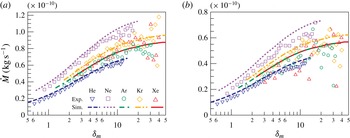
The experimental and numerical results for the mass flow rate ${\dot{M}}$ are compared in figure 1 for the two values of the temperature difference ${\rm\Delta}T$ between the reservoirs. The lines from the numerical simulation, considering full accommodation at the walls and a linear temperature distribution, show good agreement with the plots of the experimental results for the whole range of experimental conditions, i.e. from the transitional to slip flow regime, $0.5<{\it\delta}_{m}<40$ . With increasing ${\it\delta}_{m}$ , the mass flow rate increases in the transitional flow regime and asymptotically approaches a constant value in the slip flow regime. The measured results are slightly scattered in the region of large rarefaction parameter, which could be caused by very small pressure variations $|p_{\infty }-p_{i}|$ in (2.1) for both the cold and hot reservoirs due to the weak thermal creep flow, resulting in less accurate measurements of the rates of pressure variation.

Figure 1.

The experimental mass flow rate ${\dot{M}}$ is compared with the values obtained from the numerical simulations. Panel (a) is for ${\rm\Delta}T=58~\text{K}$ and (b) is for ${\rm\Delta}T=37~\text{K}$ . The symbols represent the experimental results for (▿, blue) helium, (▫, purple) neon, (○, green) argon, (♢, orange) krypton and (▵, red) xenon. The results of the simulation considering full accommodation at the walls are plotted by a dashed line for helium, a dotted line for neon, a dashed–dotted line for argon, a dashed–two-dotted line for krypton and a solid line for xenon. The maxima of the vertical axes are set in the same ratio as ${\rm\Delta}T$ for (a) : (b).

In §§ 3.2 and 3.3, it was shown by numerical simulation that under our experimental conditions the temperature-driven mass flow rate can be approximated with $0.2\,\%$ accuracy by just the term proportional to the temperature gradient ${\dot{M}}_{T}$ as in (3.5). Therefore, from (3.5), the remark above and with the help of (3.2), we can roughly approximate this temperature-driven mass flow rate as ${\dot{M}}\simeq {\dot{M}}_{T}\propto \text{d}T/\text{d}z\sim {\rm\Delta}T/L$ . In figure 1, where the experimental mass flow rate is provided, the ratio of the maxima of the vertical axes is set equal to the corresponding ratio of ${\rm\Delta}T$ , namely as 57.9 : 37.4 for the two panels (a) : (b). Thus, it is shown that the plots are quantitatively quite similar, confirming the validity of the approximation.

Let us now analyse the influence of the gas viscosity on the mass flow rate. Expression (3.7) for the temperature-driven mass flow rate as a function of ${\it\delta}_{m}$ is directly proportional to the viscosity coefficient. Furthermore, because the dimensionless mass flow rate $G_{T}$ is nearly independent of gas species for noble gases (Sharipov & Bertoldo Reference Sharipov and Bertoldo2009), (3.7) predicts that the mass flow rate is nearly proportional to the viscosity coefficient for a given value of ${\it\delta}_{m}$ . More precisely, the viscosity coefficients at the mean temperature $T_{m}$ , calculated from (2.4), are equal to 2.06, 3.29, 2.39, 2.63 and $2.40\times 10^{-5}~\text{Pa}~\text{s}$ for helium, neon, argon, krypton and xenon, respectively. As can be observed in figure 1, the mass flow rates are shown to be nearly proportional to the viscosity coefficients listed above.

Moreover, it is interesting to note that the mass flow rates for argon and xenon show quite similar values when the mass flow rate ${\dot{M}}$ is plotted as a function of ${\it\delta}_{m}$ ; see figure 1. Indeed these gas species have similar values of ${\it\mu}_{\mathit{ref}}$ (argon $2.117\times 10^{-5}~\text{kg}~\text{s}^{-1}~\text{m}^{-1}$ and xenon $2.107\times 10^{-5}~\text{kg}~\text{s}^{-1}~\text{m}^{-1}$ ) and ${\it\omega}$ (argon 0.81 and xenon 0.85), resulting in similar values not only for ${\it\mu}(T_{m})$ but for ${\it\mu}$ at every temperature. Consequently, from the previous comments, we can predict similar values for the mass flow rate of these gas species at the same ${\it\delta}_{m}$ , verified in figure 1. Let us note that, experimentally, the same ${\it\delta}_{m}$ is obtained for two gases by choosing the respective pressures such as $p_{\text{Ar}}/p_{\text{Xe}}=\sqrt{m_{\text{Xe}}/m_{\text{Ar}}}$ , following (2.5).

4.2 Influence of gas–surface interaction and temperature profile

Full accommodation of the molecules at the wall and a linear temperature profile were assumed in the numerical simulation. However, incomplete accommodation is often reported even for machined surfaces (Yamaguchi, Matsuda & Niimi Reference Yamaguchi, Matsuda and Niimi2012; Hadj Nacer et al. Reference Hadj Nacer, Graur, Perrier, Méolans and Wuest2014) and low thermal conductivity of the channel’s material might result in a nonlinear temperature profile (Rojas-Cárdenas et al. Reference Rojas-Cárdenas, Graur, Perrier and Méolans2015). To verify the relevance of these two assumptions, the effects of incomplete accommodation and of a temperature profile shape were examined numerically.

We found from the numerical results that incomplete accommodation influences essentially the mass flow rate. If ${\it\alpha}=0.8$ , which is close to the value in Rojas-Cárdenas et al. (Reference Rojas-Cárdenas, Graur, Perrier and Méolans2015), the mass flow rate increases, compared to its value for complete accommodation ${\it\alpha}=1$ , by at most 17.8 % with helium at the lowest ${\it\delta}$ . But when ${\it\delta}\gtrsim 4$ , it decreases compared to its value for ${\it\alpha}=1$ and reaches $-7.9\,\%$ at ${\it\delta}\sim 27.5$ . The tendency is similar for the other gases, but the mass flow rate deviates less from its value for ${\it\alpha}=1$ than it does for the case of helium. It was also found that the decrease in mass flow rate due to incomplete accommodation is independent of the applied temperature difference.

On the other hand, the exponential temperature profile, which is usually measured for a material with low thermal conductivity, increases the mass flow rate. If we assume the same exponential shape of the temperature distribution as that measured in Rojas-Cárdenas et al. (Reference Rojas-Cárdenas, Graur, Perrier and Méolans2015) for the microtube of circular cross-section, we find the mass flow rate to increase by at most 6.1 %, compared to the linear temperature distribution, with helium at the lowest ${\it\delta}$ . For the other gases, the impact of the shape of the temperature profile on the mass flow rate is much smaller. In general, the shape of the temperature profile exerts less influence than incomplete accommodation.

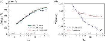
The mass flow rates in the case of full accommodation and a linear temperature profile are compared in figure 2(a) with those for incomplete accommodation and an exponential temperature profile, for argon as a typical example. The same tendency as observed above in the case of helium is clearly seen for argon in figure 2(a): the exponential temperature distribution along the channel’s wall increases the mass flow rate slightly, while incomplete accommodation increases it for the higher gas rarefaction (low ${\it\delta}$ ) and decreases it for high values of ${\it\delta}$ . To see the tendency above more clearly, the two deviations in the mass flow rate are also plotted in figure 2(b). The first deviation $({\dot{M}}({\it\alpha}=0.8)-{\dot{M}}({\it\alpha}=1))/{\dot{M}}({\it\alpha}=1)$ shows the influence of incomplete accommodation of the molecules with the channel’s wall, which leads to an increase in the mass flow rate compared to that for ${\it\alpha}=1$ for small delta and to a decrease for high ${\it\delta}$ ; see figure 2(b). The deviation of the mass flow rate due to the change in shape of the wall temperature profile $({\dot{M}}(T_{exp})-{\dot{M}}(T_{lin}))/{\dot{M}}(T_{lin})$ is positive for all ${\it\delta}$ . As can be seen from figure 2(b), the two effects of incomplete accommodation and the shape of the temperature profile compensate each other in the considered range of ${\it\delta}_{m}$ $[3,40]$ . This is probably why the numerical estimation agrees well with the experimental data (see figure 1) even though ideal conditions were assumed in the simulations. This agreement could result from the two realistic effects of incomplete accommodation and a nonlinear temperature profile varying the mass flow rate in opposite directions.

Figure 2.

The effects of the incomplete accommodation and temperature profile are evaluated by numerical simulations. In (a), the mass flow rate for the original full accommodation of the molecules at the wall and a linear temperature profile (green solid line) is plotted together with those for incomplete accommodation and a linear temperature profile (blue dashed line), and for complete accommodation and an exponential temperature profile (red dotted line); all results are for argon as a typical example. Panel (b) shows the variations, which are the differences of two effects from the original divided by the original mass flow rate. The vertical axis in (a) is modified from figure 1.

4.3 Reduced mass flow rate $G_{T}$

A simple explicit expression for the temperature-driven mass flow rate is obtained in § 3.3, (3.6). However, this expression (3.6) involves the numerical results on the coefficient $G_{T}$ . As was mentioned above, this coefficient has been calculated numerically by various authors. Therefore, we can derive the expression for $G_{T}$ from our experimental results and compare it with the available results of the numerical simulations.

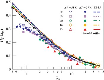
The dimensionless temperature-driven mass flow rate $G_{T}$ (see (3.6)) is plotted in figure 3 for all gases. The numerical results obtained by solving the linearized Boltzmann equation with the Lennard-Jones potential for the flow between parallel plates (Sharipov & Bertoldo Reference Sharipov and Bertoldo2009) and the numerical solution of the S-model equation with hard-sphere potential for the channel with cross-section $H/W=0.0367$ (Graur & Ho Reference Graur and Ho2014) are also plotted in figure 3. It is clear from figure 3 that the difference in gas species is very small for both the numerical and experimental results. Therefore, the reduced flow rate $G_{T}$ might be considered to be independent of gas species at least for noble gases. 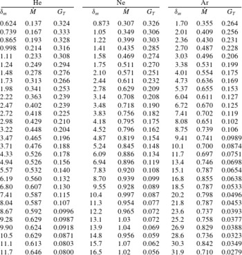The reduced flow rates $G_{T}$ of helium, neon and argon for ${\rm\Delta}T=58~\text{K}$ are listed with the measured mass flow rates in table 1.

Until the slip flow regime, the experimental results show good agreement with the numerical results. However, a small discrepancy appears in the near free molecular regime, i.e. in the region of small ${\it\delta}$ . It seems very difficult to explain this discrepancy as resulting from incomplete accommodation at the surface. As was shown in the numerical simulations (Loyalka Reference Loyalka1975; Loyalka & Hickey Reference Loyalka and Hickey1991; Sharipov & Seleznev Reference Sharipov and Seleznev1998) and through results presented here, incomplete accommodation would lead to an increase in the reduced flow rate $G_{T}$ in the region of small ${\it\delta}$ , and this is not consistent with the results in figure 3. Another possibility is that measurement errors increase with decreasing ${\it\delta}$ , because measurements are quite difficult in the regime of free molecular flow.

Figure 3.

The reduced flow rate $G_{T}$ obtained from the experimental results is plotted for both ${\rm\Delta}T=58~\text{K}$ and ${\rm\Delta}T=37~\text{K}$ . The symbols represent the experimental results for ${\rm\Delta}T=58~\text{K}$ of helium (▿), neon (▫), argon (○), krypton (♢) and xenon (▵). The data for ${\rm\Delta}T=37~\text{K}$ are plotted with filled symbols. The numerical results for the rectangular channel ( $H/W=0.0367$ ) for full accommodation, obtained by the S-model kinetic simulation in Graur & Ho (Reference Graur and Ho2014), are plotted as a dotted line with asterisks. The numerical results for the flow between two parallel plates with full accommodation and for a Lennard-Jones intermolecular potential in Sharipov & Bertoldo (Reference Sharipov and Bertoldo2009) for ${\it\delta}_{m}<10$ are also plotted as a dashed line for helium, a dotted line for neon, a dashed–dotted line for argon, a dashed–two-dotted line for krypton and a solid line for xenon.

Table 1.

The measured mass flow rates ${\dot{M}}\;(10^{-10}~\text{kg}~\text{s}^{-1})$ and reduced flow rates $G_{T}$ of typical gas species for ${\rm\Delta}T=58~\text{K}$ .

5.1 Extraction of the thermal slip coefficient from the mass flow rate

In the previous section, it was shown that in the transitional and slip flow regimes the measured mass flow rate due to thermal creep is in very good agreement with the numerical results. However, the mass flow rate can be obtained only numerically through the solution of the kinetic equation. In the previous study (Yamaguchi et al. Reference Yamaguchi, Rojas-Cárdenas, Perrier, Graur and Niimi2014), it was shown that the thermal creep phenomenon is also important in the slip flow regime. Therefore, it will be valuable to have an analytical solution in the slip flow regime (Rojas-Cárdenas et al. Reference Rojas-Cárdenas, Graur, Perrier and Méolans2015).

The flow in the microchannel in the slip flow regime could be described by the Stokes equation. As mentioned above, the pressure profile along the channel may be negligible, and the thermal creep flow could be assumed as a stationary flow at $t=0$ where the mass flow rate is calculated; thus, the equation has the form

where the $z$ -axis coincides with the direction of the temperature gradient and the thermal creep flow is induced in the $z$ direction with velocity $u_{z}$ . The thermal slip boundary condition on a flat wall has the form

where ${\it\rho}$ is the gas density. The solution of the Stokes equation, (5.1), with the thermal slip boundary condition, (5.2), is a constant velocity over the whole cross-section (Sharipov Reference Sharipov2011). Thus, the mass flow rate is obtained as

By using (2.4) for the viscosity coefficient, the mass flow rate is expressed as

where $\mathscr{F}=T^{{\it\omega}-1}\,\text{d}T/\text{d}z$ , and only $\mathscr{F}$ varies with local conditions. It was pointed out in § 4.1 that in this study the temperature profile along the channel was not measured; therefore, the mean value of $\mathscr{F}$ was calculated by integrating its expression along the channel:

so we do not need to make any assumption about the shape of the temperature distribution.

The thermal slip coefficient ${\it\sigma}_{T}$ was calculated from the measured mass flow rate by using the analytical expression for the mass flow rate due to thermal creep, (5.4) and (5.5):

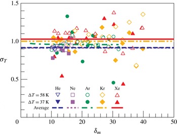
The calculated thermal slip coefficient ${\it\sigma}_{T}$ , obtained in the slip flow regime, ${\it\delta}_{m}=[10,40]$ , is plotted in figure 4. To validate the independence of the coefficient ${\it\sigma}_{T}$ from ${\it\delta}_{m}$ , it is plotted against ${\it\delta}_{m}$ . 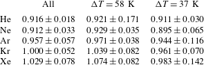The plot is a little scattered as a result of the scattered results of the mass flow rate discussed in § 4.1, but the value seems to be independent of the rarefaction parameter ${\it\delta}_{m}$ and of the temperature difference ${\rm\Delta}T$ as in Rojas-Cárdenas et al. (Reference Rojas-Cárdenas, Graur, Perrier and Méolans2015). Therefore, the obtained results are averaged over the two temperature differences and they are listed in table 2 as ‘all’ and plotted with horizontal lines in figure 4. The 95 % confidence interval for the averaging is listed as errors in table 2. To see the effect of the temperature difference, the averaged values for each ${\rm\Delta}T$ are also listed in table 2. The differences among ‘all’, ${\rm\Delta}T=58~\text{K}$ and ${\rm\Delta}T=37~\text{K}$ are very small and within the error interval. It is important to note that the number of the data in the range used for the averaging was different for every gas species, since the rarefaction parameter ${\it\delta}$ , (2.3), is different between gas species at the same pressure due to the difference in molecular weight.

Figure 4.

The thermal slip coefficients ${\it\sigma}_{T}$ obtained from the experimental results are plotted for ${\rm\Delta}T=58~\text{K}$ and ${\rm\Delta}T=37~\text{K}$ . They are plotted against ${\it\delta}_{m}$ , validating that the coefficient is independent of ${\it\delta}_{m}$ . The symbols represent the experimental results for ${\rm\Delta}T=58~\text{K}$ of helium (▿), neon (▫), argon (○), krypton (♢) and xenon (▵). The data for ${\rm\Delta}T=37~\text{K}$ are plotted with filled symbols. The values averaged over the two ${\rm\Delta}T$ cases are plotted as a dashed line for helium, a dotted line for neon, a dashed–dotted line for argon, a dashed–two-dotted line for krypton and a solid line for xenon.

Table 2.

Thermal slip coefficients obtained from the averaged mass flow rate over the range of ${\it\delta}_{m}=[10,40]$ . The errors are the 95 % confidence interval of the fitting procedure.

5.2 Extraction of ${\it\sigma}_{T}$ by an asymptotic expression for the mass flow rate

The above-mentioned mass flow rate, obtained by solving the Stokes equation with the thermal slip boundary condition, is a first-order solution. The higher-order solution for the dimensionless temperature-driven mass flow rate $G_{T}$ was obtained from the kinetic theory in the form of an asymptotic expression in Loyalka & Hickey (Reference Loyalka and Hickey1989); in terms of the dimensional mass flow rate, it reads

where the coefficients $A^{T}$ and $B^{T}$ as obtained by Loyalka & Hickey (Reference Loyalka and Hickey1989) are $A^{T}=0.9924$ and $B^{T}=-1.3284$ . It should be noted that here, as previously, the pressure gradient is assumed to be small and only the term with the temperature gradient is retained. By comparing (5.3) and (5.7), it is clear that the two expressions are similar and $A^{T}$ can be identified as the thermal slip coefficient ${\it\sigma}_{T}$ in the slip flow regime. However, the asymptotic expression (5.7) contains the additional term of the order of $O(1/{\it\delta})$ and therefore allows the coefficient ${\it\sigma}_{T}$ to be determined more accurately. As in the case with the first-order extraction, expression (5.7) was integrated along the channel by using the property of mass conservation. To integrate expression (5.7), the rarefaction parameter ${\it\delta}$ was also related to the mean rarefaction parameter ${\it\delta}_{m}$ and the local temperature and pressure values; see Rojas-Cárdenas et al. (Reference Rojas-Cárdenas, Graur, Perrier and Méolans2015) for more details. Finally, the expression for the mass flow rate in terms of the mean value and the values in the reservoirs is obtained:

The previous expression, by analogy with (5.6), can be rewritten in the following form:

It is clear that the measured mass flow rate can be fitted in the form of (5.9) and the fitting coefficient $A^{F}$ can be associated with the coefficient ${\it\sigma}_{T}$ .

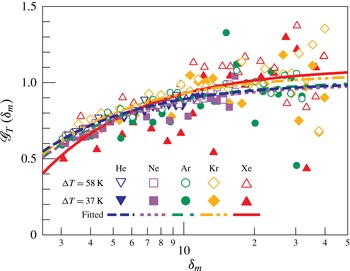
Since the asymptotic expression allowed the applicable flow regime to be enlarged to the transitional flow regime, the measured mass flow rate in the range of ${\it\delta}_{m}=[3,40]$ was employed for the fitting procedure. The experimental data with the fitting curves are plotted in figure 5. The coefficients $A^{F}$ and $B^{F}$ , obtained from the fitting of the experimental data according to (5.9), are listed in table 3. The coefficient $B_{2}$ was quite close to unity and the largest deviation from unity was less than 0.1 %. Therefore, $B_{2}=1$ was assumed to calculate the thermal slip coefficients from all the data for both ${\rm\Delta}T=58~\text{K}$ and ${\rm\Delta}T=37~\text{K}$ . The errors from $B_{2}$ in the calculation of the coefficient $B^{F}$ were also neglected, since the values were almost constant and the errors in the temperature measurement should be very small.

Figure 5.

$\mathscr{G}({\it\delta}_{m})$ given by (5.9) is plotted as a function of ${\it\delta}_{m}$ , obtained from the experimental results, for ${\rm\Delta}T=58~\text{K}$ and ${\rm\Delta}T=37~\text{K}$ . The symbols represent the experimental results for ${\rm\Delta}T=58~\text{K}$ of helium (▿), neon (▫), argon (○), krypton (♢) and xenon (▵). The data for ${\rm\Delta}T=37~\text{K}$ are plotted with filled symbols. The fitting curves over both ${\rm\Delta}T$ cases are plotted as a dashed line for helium, a dotted line for neon, a dashed–dotted line for argon, a dashed–two-dotted line for krypton and a solid line for xenon.

These results are theoretically much more reliable than the first-order extraction in table 2, because a greater number of data were employed for the fitting procedure, which is especially true for helium. In addition, the values are quantitatively in quite good agreement with the numerical (Sharipov & Bertoldo Reference Sharipov and Bertoldo2009) and experimental results in the literature (Annis Reference Annis1972; Porodnov et al. Reference Porodnov, Kulev and Tuchvetov1978; Rojas-Cárdenas et al. Reference Rojas-Cárdenas, Graur, Perrier and Méolans2015). This agreement indicates notably that the thermal slip coefficient is independent of the cross-sectional shape of the channel.

Table 3.

Thermal slip coefficients $A^{F}$ and $B^{F}$ obtained by the fitting of the expression for the asymptotic mass flow rate over the range of ${\it\delta}_{m}=[3,40]$ . $B_{2}$ was assumed to be unity in the calculation for ‘all’. The errors show the 95 % confidence interval of the fitting procedure, and uncertainties from $B_{2}$ are neglected.

Comparing between gas species, the thermal slip coefficient increases with increasing molecular weight, except for neon, which gives a slightly smaller value than helium. It shows the same tendency as the case of first-order extraction, see table 2. This tendency is exactly the same with the numerical results (Sharipov Reference Sharipov2011) and with the experimental values obtained previously in Annis (Reference Annis1972) and Porodnov et al. (Reference Porodnov, Kulev and Tuchvetov1978).

As is clear from table 3, the coefficients $B^{F}$ are also close to the value $B^{T}=-1.3284$ , obtained numerically in Loyalka & Hickey (Reference Loyalka and Hickey1989) under the assumption of complete accommodation. The comparison between the experimentally obtained coefficients and the numerical data, especially for the coefficient $B^{T}$ , which is more sensitive to the accommodation coefficient (Loyalka & Hickey Reference Loyalka and Hickey1989), indicates that the experimental accommodation coefficient is not so far from unity.

It would also be interesting to calculate the accommodation coefficient from the thermal slip coefficient obtained experimentally, by using, for example, the following expression proposed in Sharipov (Reference Sharipov2011) in the frame of the Maxwell diffuse–specular boundary condition and using the S-model kinetic equation:

However, the thermal slip coefficient is very sensitive to the type of kinetic equation (S-model kinetic equation or Boltzmann equation) used for its numerical calculation, and especially to the implemented intermolecular potential (hard-sphere model, Maxwellian molecules, Lennard-Jones potential). In the case of full accommodation at a surface, the values of ${\it\sigma}_{T}$ are dispersed for different potentials within 16 %, as stated in Sharipov (Reference Sharipov2011). The same problem appears when trying to simulate diffuse–specular scattering: the disagreement between the results obtained by the variational method applied to the S-model with diffuse–specular boundary conditions and the solution of the Boltzmann equation with the HS potential varies from 3 % for ${\it\alpha}=0$ to 12 % for ${\it\alpha}=1$ (Sharipov Reference Sharipov2011).

Moreover, when one extracts an experimental value of the accommodation coefficient from the thermal slip coefficient by using (5.10), it is clear that the uncertainties on ${\it\alpha}$ represent $8/3$ of the uncertainties on ${\it\sigma}_{T}$ and so would lie beyond the acceptable accuracy, especially for argon and xenon. In addition, taking into account this large difference in numerical values of ${\it\sigma}_{T}$ described above, the implementation of (5.10) itself to extract the value of the accommodation coefficient can engender a large additional error. Therefore, it is not reasonable to calculate the accommodation coefficient from the experimental results in this study. Nonetheless, the accommodation coefficient that corresponds to the obtained thermal slip coefficient would be not so far from unity, which is consistent with the above-mentioned characteristics from the $B^{T}$ coefficient.