Introduction

Because the presence of an ice cover modifies the exchanges of energy and mass between the ocean and atmosphere, it is an important component of the climate system. Early estimations, such as those of Fletcher (1969), demonstrated the impact that a continuous sea-ice cover has on the ocean-atmosphere energy exchange within the entire Antarctic sea-ice zone. However, this zone is actually composed of a mixture of different types and thicknesses of ice, plus open water in the form of leads and polynyas, and is not a region of uniform ice of constant thickness. Heat loss from small areas of open water can greatly increase the total energy exchange and, as noted by Maykut (1978), heat losses over thin ice are also substantial and important in any calculation of the overall surface heat balance. Wellcr (1980) partly allowed for the non-uniform nature of the Antarctic sea-ice zone by dividing the pack into an inner and outer zone characterized by an areal ice concentration (C) of C ≥ 85% and 15% ≤ C < 85%, respectively. His inner zone was estimated to consist of 10% open water, 10% 0-40 cm thick ice and 80% > 40 cm thick ice, whereas the outer zone had percentages 40, 20 and 40, respectively. Weller calculated the total heat flux for each zone as a linear mix of the fluxes for each type of surface and did not take account of non-linear effects arising as a result of the internal boundary layer which is established immediately downwind of a change in surface conditions. The average mid-winter fluxes of turbulent sensible and latent heat over the entire Antarctic pack ice in this model are as much as a factor of six greater than Fletcher’s estimates.

Recent studies of ice concentration and thickness in the Antarctic show that a much larger area of the pack is made up of young, thin, first-year ice than previously thought. Gow and others (1982) showed that up to 50% of the total ice column of the Weddell Sea pack consisted of aggregated frazil crystals formed in leads and polynyas and Wadhams and others (1987) estimated a mean ice thickness of between 0.3 m and 0.6 m around 0° longitude in winter. In the Indian Ocean sector, although the average ice concentration in the spring is as high as 80%, much of the ice is young, thin ice and Allison (1989) estimated an area-weighted thickness of less than 0.4 m. This is supported by Brandt and others (1990), who estimated that more than 20% of the area within the spring pack consists of largely snow-free ice less than 0.3 m thick, and that a further 30% is less than 0.7 m thick. Jacka and others (1987) also found large areas of young, thin ice and frazil in the pack off East Antarctica, whereas Southern (1989) noted that most of the ice in the area south of 57°S along the meridians 78°E and 75°E was thin to medium first-year ice intermixed with immature ice thinner than 0.05 m.

In this paper, we explore the consequences that such a large percentage of thin ice, even in Weller’s inner zone, has on the overall energy budget between ocean and atmosphere. We consider particularly the turbulent fluxes and include consideration of the non-linear variation of the total turbulent flux with ice concentration.

Energy Exchange Over thin Antarctic Sea Ice

The surface energy budget of snow-free sea ice can be expressed as

where F_r represents incoming solar radiation, α the surface albedo, I_o the fraction of short-wave radiative energy penetrating into the ice, F_li the incoming long-wave energy, F_lo the emitted long-wave energy, F_s the turbulent sensible heat flux, F_e the turbulent latent heat flux and F_c the conducted heat flux. A negative value indicates that the surface acts as a heat source; a positive value indicates a heat sink.

Maykut (1978) derived a single-layer thermodynamic model of thin sea ice based on the multi-layer model of Maykut and Untersteiner (1971). He expressed sensible and latent turbulent fluxes in bulk aerodynamic form, as

The conducted flux, in terms of a salinity-dependent thermal conductivity, is

and the emitted long-wave energy is

Here, the latent and sensible heat transfer coefficients, C_L and C_s , respectively, have the values 1.75 x 10⁻³ and 3.0 X 10⁻³, the Stefan-Boltzman constant σ = 5.6687 x 10⁻⁸, the conductivity of pure ice k_o = 2.03 Wm⁻¹ K⁻¹, the long-wave emissivity of the surface ∊ = 0.96, the latent heat of sublimation L_s = 2.8 x 10⁶6⁻¹, the specific heat of air at constant pressure c_p = 1004 Jkg⁻¹K⁻¹, the average air density ρ= 1.3 kg m⁻³, and the temperature at the lower surface of the ice T_b = −1.8°C. The a, b, c, d and e′ are constants in an empirical relationship for saturation vapour pressure as a function of T_a . β 0.117Wm⁻²kg⁻¹ is a constant. T_o is surface temperature (K), T_a air temperature (K), S_o salinity of the ice (parts per thousand),f relative humidity (%), p₀ atmospheric pressure (hPa), H ice thickness (m), and u is wind speed (ms⁻¹).

From Equations (1) to (5), Maykut (1978) obtained a fifth degree polynomial solution for T_o in terms of prescribed values of F_r,F_li,T_a,u,f and H. Values of the turbulent, conducted and emitted long-wave radiation fluxes over thin ice were then obtained from Equations (2), (3) and (4). A major assumption of this single-level thin-ice model is that the temperature gradients within the ice are linear; i.e. the ice essentially has zero heat capacity. This docs not apply for thicker ice (Maykut suggests ≥ 0.8 m) where temperature gradients have considerable curvature.

We have used Maykut−s (1978) model, with input values typical of what we expect for the Antarctic sea-ice zone in September, to estimate heat fluxes over thin Antarctic sea ice. Incoming short-wave radiation is set to 70 Wm⁻² based on coastal Antarctic observations (e.g. Weller, 1967) and incoming long-wave radiation is estimated as

where e_a is an effective emissivity, derived by Brunt’s formula (after Zillman, 1970) from surface air temperature and humidity, and the constant 1.38 is a cloudiness correction (Budyko, 19G3) for a typical low-level cloud cover for latitudes 60° −65−S in September of 4/8 (Warren and others, 1988). F_li ranges from 200 Wm⁻² at −20°C (253.2K) to 2G5Wm⁻² at 5°C (268.2K). Based on Jenne and others (1974) and Zwally and others (1983), we assume an average wind speed for September of 8 ms⁻¹ and an atmospheric pressure of 980 h Pa. Surface relative humidity is taken as 90% and air temperature is treated as a sensitivity parameter in the range −5° to −20°C (Jenne and others, 1974). All other variables and constants are the same as those used by Maykut for the central Arctic, including albedo and salinity values as a function of ice thickness, and a value of I_o of 0.17. The fifth degree polynomial expression for T₀ was solved using Laguerre’s method (e.g. Press and others, 1986: 263-266).

The values of the computed heat fluxes as a function of both air temperature and ice thickness are shown in Figure 1, and the strong dependence of the turbulent fluxes on ice thickness is shown in Figure 2 for air tem-peratures of −10° and −20°C. At −10°C, the sensible heat component is the dominant mechanism of total turbulent loss for all but the thicker ice and, since the latent term changes little with temperature, sensible loss is even more important at 20°C. At −5°C, however, the latent flux is similar or greater than the sensible flux.

Turbulent Heat Loss from Leads and Polynyas

When air blows over a solid-ice or ice-covered surface and suddenly encounters an area of open water, such as a lead or polynya, it experiences both an abrupt change in surface roughness and a dramatic change in surface temperature. Over ice in winter, the surface air temperature will be very close to that of the ice itself which, in the case of first-year Antarctic sea ice of 0.4 m thickness, will be approximately −15°C. In contrast, the water temperature will be at the freezing point, a relatively warm −1.8°C. As a result, intensive turbulent mixing takes place over water as wind, which has been blowing over the ice, suddenly encounters these changes in surface characteristics. This dramatically increases the

Fig. 1.

Variation in the energy balance components at the surface of thin sea ice with temperature and ice thickness, F_s, is the sensible heat flux. F_e is the latent heat flux. F_c is the heat conducted within the ice and F_lo the emitted long-wave radiation. The vertical .scale is different for each component.

Fig. 2.

Variation of turbulent heat flux with ice thickness.

magnitude of the turbulent heat fluxes from the surface to the atmosphere. As the air proceeds downwind from the step-change in conditions and is gradually heated, a thermal internal boundary layer forms acting to reduce air-water temperature differences and fluxes. The significant change in heat fluxes immediately downwind of any changes in surface roughness or temperature means that the average heat flux from a lead is fetch dependent. Hence, lead widths must be known to properly estimate the overall heat budget of the pack, and treating the total heat loss simply as a linear mix of heat fluxes over different surfaces is a poor approximation.

Andreas and others (1979) conducted a number of experiments during the AIDJEX Lead Experiment, over both natural and artificial leads up to 35 m wide. They estimated sensible heat flux upwind and downwind of leads of various widths from measured wind and temperature profiles. Using similar experimental data for the evaporative flux (Andreas, 1982), Andreas (1980) derived an empirical relationship for the estimation of turbulent heat fluxes over leads from bulk quantities

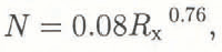
where N, the Nusselt number, is the non-dimensionalised heat flux and R_x is the fetch Reynolds number. Andreas and others (1979) define the fetch Reynolds number as

where U ₂₀₀ is the wind speed 200 cm above the upwind surface and v is the kinematic viscosity of air (1.334 x 10m²s⁻¹). Downwind fetch is symbolised as x.

The Nusselt numbers for sensible (N_s ) and latent heat (N_L ) are defined as

and

where F_s and F_e. are the average sensible and latent heat losses from the lead, T₂₀₀ and Q₂₀₀ the temperature and specific humidity 200 cm above the upwind surface, T_w is the temperature of the downwind surface, Q₀ the specific humidity of air in saturation with a surface at temperature T_w, L_v the latent heat of vapourization (2.5 x 10⁶Jkg⁻¹), D_w the molecular diffusivity of water (2.24 x 10⁻⁵m²s⁻¹ at −1.8°C) and k is the thermal conductivity of air (2.43 x 10⁻²Jm¹ at −1.8°C). Using additional measurements made downwind of Arctic polynyas, Andreas and Murphy (1986) showed that the above relationships are valid for fetches of up to 500 m.

We use these equations to estimate the average value of the turbulent heat fluxes over an open water lead of fetch x, under the same wind and temperature conditions considered in the section on energy exchange over sea ice. The total turbulent loss over the open water lead,

is shown in Figure 3. This illustrates the rapid change in average heat flux with lead width for narrow leads, but, as lead width increases, the air mass approaches equilibrium and the rate of change with fetch decreases. The relative contribution of the two components is given by the Bowen ratio (F_s/F_v), which varies from approximately 1.7 at −5°C, to approximately 3.5 at −20°C.

Fig. 3.

Variation in the total turbulent heat transfer over leads of varying fetch, for differentambient air temperatures from −5° to −20°C.

Turbulent Exchange Over Young Pack of Varying Concentration

Having calculated the turbulent heat transfer over thin, snow-free ice and over water surfaces, respectively, it is possible to estimate the total turbulent exchange of heat over a large area within the Antarctic pack, if we assume it to be a mix of both ice floes and Leads. To do this fully, the ice-thickness distribution, as well as floe size (lead width) and meteorological variables such as air temperature and wind speed, must be known. However, since there are virtually no data from which these parameters can be determined, other than shipboard observations which arc sparse and randomly located, we consider here only young pack ice of vuying concentration consisting of floes of uniform ice thickness and a constant size of 100 m, which is typical of the East Antarctic pack away from the ice edge (e.g. Jacka and others, 1987; Allison, 1989).

The turbulent transfer of heat from ocean to atmosphere can be calculated by linearly summing the relative heat-flux contributions from each surface within the sea-ice zone, using the results of the previous sections. Hence, for a single ice thickness category, the average turbulent heat flux (F_T) is given by

where F _I is the fractional contribution to the turbulent flux from the ice covered area and FL the fractional contribution from open water (leads).

To simulate varying conditions of ice cover, we assume that the pack is infinitely uniform across wind, and that downwind it is composed of constant width floes (100 m) interspersed with open-water leads of different width, as shown in Table 1. The non-linear change of sensible and latent heat flux associated with a step change in the boundary layer over open water has been accounted for in the previous section. We are, however, only considering a “single lead” system, neglecting the cumulative effect uf modification of the air mass as it passes over a succession of leads and the similar fetch-dependence of the heat loss over ice.

The calculated contribution from over the ice and the leads, and the area-averaged total turbulent heat loss for pack ice of concentration 100, 80, 65, 50 and 30%, are shown as a function of different ice thickness and

Table 1.

Floe and lead dimensions used to simulate pack ice of different concentrations.

Table 2.

Area-averaged total turbulent heat flux ( Wm⁻²) over pack ice of different concentration as a function of air temperature and ice thickness (H). F_I is the fractional contribution to the turbulent flux from the ice-covered area, F_L the fractional contribution from open water (leads), and F_T the average turbulent flux over the total region. The lead width used for each concentration category is given in Table 1.

air temperature in Table 2. Consider first the results for an ice concentration of 80%, typical of the average concentration off East Antarctica in September. At an air temperature of −10°C, the turbulent heat flux over ice 0.4m thick is −38Wm⁻², whilst the turbulent flux over a 25 m lead is 300 Wm⁻². Hence, from Equation 12, the total average turbulent flux for 80% concentration ice is −90Wm⁻². A decrease in ice thickness to 0.2 m increases the turbulent flux over the ice surface to −63Wm⁻² and the average flux over the region of 80% concentration to −lllWm⁻². A further decrease in H to 0.1 m causes an even larger increase in F_T in response to the larger changes in ocean-atmosphere heat exchange over the thinnest categories of ice. For this ice thickness, the average turbulent heat flux over the region is −142 Wm⁻². These, and the results for other ice thicknesses and air temperatures, are shown in Figure 4. Note that the turbulent heat flux over ice of only 0.1 m thickness varies markedly, depending on air temperature, with a range from −53Wm⁻² at −5°C to −224Wm⁻² at −20°C. The flux over this very thin ice, regardless of the air temperature, is the major contributor to the area-averaged turbulent heat flux for an ice concentration of 80%. That is, the turbulent heat flux over 100 m of 0.1 m thick ice exceeds that over a 25 m lead.

Fig.4.

Variation in the, average turbulent heat flux over an ice-water surface of 80% concentration, where floe size equals 100 m and lead size egaals 25 m. The heat flux is shoum for a range of ice thicknesses from 0.1m to 0.8 m.

As ice thickness increases, F_L rapidly becomes dominant, although the area-averaged total turbulent heat flux begins to decrease. An increase in H from 0.1m to 0.2 m shows how rapidly the contribution of F _L falls as the ice thickens. For H = 0.2 m, the contribution of F_I already exceeds that of F_L for air temperatures below −5°C, and for 0.4 m thick ice the contribution from the leads at colder temperatures is about double that from the ice-covered area. However, the turbulent heat transfer over 0.4 m thick ice is by no means negligible, and makes an important contribution to the total turbulent heat exchange (F_T) in the sea-ice zone. It is clear that at 80% concentration, and for conditions where there are extensive areas of thin ice (as observed in the Antarctic), the turbulent fluxes over the ice may contribute to the total heat budget of the region on a scale similar to that of the turbulent fluxes over open water.

The total turbulent heat losses for other ice concentrations, using the assumptions in Table 1, are given in Table 2. As expected, the decrease in concentration generally results in an increase in FT for each thickness of ice because of increased heat loss from leads. (The apparently greater flux for 50% compared to 30% ice of 0.1 m thickness occurs because the turbulent fluxes from wide leads calculated by Equations (9) and (10) are not completely identical to the open-water loss calculated using the bulk aerodynamic assumptions of the section on energy exchange.) In our model, the turbulent heat loss (per unit area) from floes has no fetch dependence and is not altered by changes in ice concentration. However, as concentration decreases, the turbulent fluxes over the ice contribute less to the total heat flux of the region. Over leads, the turbulent heat fluxes at any point, x, remain constant despite changes in ice concentration or distribution, but the average flux over leads varies considerably and non-linearly as the leads increase. Whilst decreasing concentration (increasing lead width) causes a decrease in the average turbulent heat flux per unit area from the open water, there is, as a result of the larger area of open water, an increase in the total flux.

Figure 5 shows the variation in F_T with changing ice concentration for an air temperature of −10°C. The non-linear nature of the relationship between concentration and the total turbulent transfer of heat is clearly

Fig. 5.

Variation in the average turbulent heat flux over a mixed ice- water surface as a function of ice thickness and ice concentration, at an air temperature of −10°C. The heat flux is shown for a range of ice thicknesses from 0.1 m to 0.8m.

illustrated. As concentration decreases from 100% ice cover to 80%, there is a rapid change (of approximately 50Wm⁻²) in the loss of turbulent heat to the atmosphere. The rate of increase of F_T slows as concentration is further decreased and the turbulent heat fluxes from the open water have a lesser effect on the total area-averaged flux. This is because a decrease in concentration is effectively only increasing lead width and the air over the “additional” water has already been modified by the water surface immediately upwind. This serves to highlight the importance of air modification over leads and the necessity of taking account of these processes in heat flux calculations.

Discussion and Conclusions

In considering the results presented above, it is important to keep in mind the limitations of the simple model used. First, we have considered only thin ice (<0.8m) of uniform thickness. Whereas the observations of Brandt and others (1990) in the Indian Ocean sector show that, at a distance from the ice edge greater than 500 km, about 30% of the pack is thicker than 0.7 m, the greater percentage of thin ice will be much more important in determining the total turbulent transfer of heat. We also consider only snow-free ice but even 2 or 3 cm of snow on thin ice can have a large effect on surface temperature and, hence, on the turbulent fluxes. However, Brandt and others (1990) observed that ice less than 0.15 m thick was almost always snow-free, and that ice between 0.15 and 0.3 m was either snow-free or had a snow cover of less than 0.03 m. Therefore, the assumption of snow-free ice is probably not unreasonable as a first step for determining the impact of extensive areas of thin ice on the turbulent heat exchange.

More importantly, in estimating the effect of concentration on total heat loss, we have considered only a con-stant floe size of 100 m. If a different flow size, and appropriate lead widths, were taken then the magnitude of the estimated fluxes would change somewhat. With smaller floes and narrower leads, the loss from the leads is greater and the area-averaged heat flux increases more rapidly with a concentration decrease from 100%. With large floes and wider leads, the opposite occurs but, in both cases, the sensitivity of the total heat loss to concentration change remains greatest at high concentrations and approaches zero below 50%. In part, the sensitivity of the results to the assumed floe size arises because of another of our assumptions. We consider only a “single-lead” system and do not allow for the cumulative effect of passage over successive leads and floes, nor for a fetch dependence on the turbulent heat loss over the floes. Qualitatively, the cumulative modificiition of the air mass would tend to decrease the total flux, particularly at higher concentrations and for narrower leads, counteracting the effect of a decrease in the assumed flow size.

Apart from temperature, which is treated as a sensitivity parameter, we consider only one set of climatic forcing. Thus, while it is not totally appropriate to make comparisons, our results are nevertheless in general agreement with other studies for similar ice conditions. For example, Weller (1980) estimated a mid-winter turbulent loss of −117Wm⁻² over his inner Antarctic zone (80% 0.8 m thick ice plus 10% 0.2 m thick ice). Our results for 90% 0.8 m thick ice give a total loss of −105Wm⁻² at −20°C and −54Wm⁻² at −10°C. Over his outer zone (40% 0.8 m thick ice, plus 20% 0.2 m thick ice), Weller estimated a flux of 189 Wm⁻², whereas for G0% 0.8m thick ice our turbulent loss is −108Wm⁻² at −10°C and −205Wm⁻² at −20°C.

Despite the limitations of the model, the results of this sensitivity study do show a number of additional features that we might expect intuitively. Of major importance is the indication that, if the Antarctic pack contains as much thin ice as recent observations suggest, the heat loss through this thin ice is significant compared even to the loss over open water. At 80% ice concentration the turbulent heat loss through thin ice can be greater than that from open water. As concentration decreases, however, the fractional loss through the ice and, hence, the thickness of the ice, becomes less significant. This is in sharp contrast to the situation in the central Arctic, where Maykut (1982) calculated area-weighted total turbulent heat loss taking account of the ice-thickness distribution. For March he estimated that less than 8% of the pack was open water or thin ice and the total turbulent transfer was dominated by transfer over the large area of thick ice.

Secondly, changes in ice concentration or in ice thickness both significantly modify the turbulent energy exchange over high concentration pack ice but, for ice concentration less than about 50%, there is effectively no change in the total turbulent heat loss for a change in concentration. At the same time, the effect of ice thickness becomes less important at low concentration since the heat lost through the floes represents a decrcasingly significant percentage of the total.