1. Introduction
Interfacial instabilities occur in many multi-layer flows present in processes of industrial significance, such as solvent extraction, coating and oil recovery, and may lead to important changes in the heat and mass-transfer properties of the system. Interfacial waves in vibrated containers have received much attention in the literature, largely focused on Faraday waves which are excited by vertical vibrations. Vibrations that are normal to the interface differ qualitatively from tangential vibrations; the former affect the fluid by changing the effective gravity and, thus, the hydrostatic pressure gradient, whereas the latter induce a sheared flow altering the interface stability properties. Horizontally excited waves have received less attention because they are resistant to analysis.
The effect of horizontal vibrations on two superposed immiscible liquids has been examined both experimentally (Wolf Reference Wolf1969, Reference Wolf1970; Ivanova, Kozlov & Evesque Reference Ivanova, Kozlov and Evesque2001; Talib, Jalikop & Juel Reference Talib, Jalikop and Juel2007; Mialdun et al. Reference Mialdun, Ryzhkov, Melnikov and Shevtsova2008; Jalikop & Juel Reference Jalikop and Juel2009; Yoshikawa & Wesfreid Reference Yoshikawa and Wesfreid2011b ) and theoretically (Lyubimov & Cherepanov Reference Lyubimov and Cherepanov1987; Khenner et al. Reference Khenner, Lyubimov, Belozerova and Roux1999), where it was shown that if the state of the flat contact line is unstable, non-propagating periodic waves may occur on the interface. Following Wunenburger et al. (Reference Wunenburger, Evesque, Chabot, Garrabos, Fauve and Beysens1999), these waves, which are stationary in the reference frame of the vibrated cell, are referred to as ‘frozen waves’.
By means of linear stability analysis Lyubimov & Cherepanov (Reference Lyubimov and Cherepanov1987) predicted that in the limit of high frequencies
 ${\it\omega}=2{\rm\pi}f\gg H^{2}/{\it\nu}$
(the period of vibrations is much smaller than the viscous time scale), and vanishing amplitudes of forcing
 $A\ll H$
, the interface between two liquid layers of equal thickness,
 $H$
, becomes linearly unstable to a sinusoidal disturbance when
 $$\begin{eqnarray}{\rm\Delta}U^{2}>\frac{2({\it\rho}_{1}+{\it\rho}_{2})}{{\it\rho}_{1}{\it\rho}_{2}}\left(\frac{2{\rm\pi}{\it\sigma}}{{\it\lambda}}+\frac{({\it\rho}_{1}-{\it\rho}_{2})g}{2{\rm\pi}/{\it\lambda}}\right)\tanh (H2{\rm\pi}/{\it\lambda}),\end{eqnarray}$$
where
 ${\it\rho}_{1},{\it\rho}_{2}$
are the density of liquids,
 ${\it\nu}$
is the kinematic viscosity,
 ${\it\sigma}$
is the surface tension and
 ${\it\lambda}$
is the wavelength. This relation was obtained for inviscid fluids and corresponds to the state when the mean motion in the bulk is absent but the interface oscillates with a small amplitude with respect to the amplitude of the frozen waves. In order to examine the stability of a flow which occurs in vessels of finite length, they imposed the conservation of horizontal volume flux. The velocity difference between the layers can be written as (e.g. see Khenner et al.
Reference Khenner, Lyubimov, Belozerova and Roux1999)
 $$\begin{eqnarray}{\rm\Delta}U=\frac{2({\it\rho}_{1}-{\it\rho}_{2})}{({\it\rho}_{1}+{\it\rho}_{2})}A{\it\omega}.\end{eqnarray}$$
The relation (1.1) is analogous to the dispersion relation of the basic instability mode of Kelvin–Helmholtz (K–H) type for two counter flows when
 ${\rm\Delta}U/\sqrt{2}$
is regarded as the velocity difference in the K–H case. Horizontal vibrations applied to a cell with two superimposed liquids generate a horizontal pressure gradient that induces oscillatory shear flows. The specificity is that, as a result of a harmonic change in the flow direction, the wave remains on average in the same place, as its profile is frozen in the reference frame of a vibrating container.
Khenner et al. (Reference Khenner, Lyubimov, Belozerova and Roux1999) extended the inviscid analysis of Lyubimov & Cherepanov (Reference Lyubimov and Cherepanov1987) to arbitrary amplitudes (dropping the limitation
 $A\ll H$
) and considered the inviscid case and the case of equal kinematic viscosities of two fluids. The inviscid stability boundary was obtained by Floquet analysis of the Mathieu equation which comprises a succession of tongues of harmonic response, i.e. of the same period as that of the external oscillatory drive. In addition to the K–H instability, they found regions of parametric instability associated with the intensification of capillary-gravity waves at the interface. They reported that viscosity has a weak influence on K–H type instability but strongly damps parametric instability.
Subsequent studies of vibrating fluids were aimed at clarifying the role of viscosity. Ivanova et al. (Reference Ivanova, Kozlov and Evesque2001) and Gandikota et al. (Reference Gandikota, Chatain, Amiroudine, Lyubimova and Beysens2014a ) reported a favourable agreement of measurements for the onset of interfacial instability with the inviscid theory. Another group of authors (Talib & Juel Reference Talib and Juel2007; Talib et al. Reference Talib, Jalikop and Juel2007; Jalikop & Juel Reference Jalikop and Juel2009) carried out experiments and a linear stability analysis of two immiscible liquids for a very large range of viscosity contrasts between layers. They reported that Kelvin–Helmholz mode instability was hardly influenced by the viscosity for fluid layers with a small viscosity contrast, while a substantial decrease of the instability threshold was found in fluid layers with a large viscosity contrast. They demonstrated that for finite frequencies of vibration, the inviscid model (Lyubimov & Cherepanov Reference Lyubimov and Cherepanov1987) underestimates the threshold for fluids of equal viscosities, but overestimates the threshold for fluids with a large viscosity contrast.
The stability of two superposed immiscible liquids in a axisymmetric geometry was studied numerically (Yoshikawa & Wesfreid Reference Yoshikawa and Wesfreid2011a ) and experimentally (Yoshikawa & Wesfreid Reference Yoshikawa and Wesfreid2011b ). The vibrational motion was imposed by alternating the rotation of a container around its axis. Similar to the previous authors, their linear stability results exhibit significant influence of the viscosity contrast on the stability threshold. Their experimental results for liquids, whose viscosities differ by 10 000 times, were favourably compared with the prediction by the linear stability analysis in the case of small-amplitude oscillations.
In the present study we are interested in miscible fluids, when surface tension vanishes. Recent experiments (Pojman et al. Reference Pojman, Whitmore, Liveri, Lombardo, Marszalek, Parker and Zoltowski2006; Lacaze et al. Reference Lacaze, Guenoun, Beysens, Delsanti, Petitjeans and Kurowski2010) presented evidence of the existence of a transient surface tension between two miscible fluid phases. The idea that the miscible interface should be endowed with a dynamic surface tension was first raised by Korteweg, and then developed by Zeldovich (Reference Zeldovich1949) and others. The fact that miscible liquid/liquid interfaces possess surface tension similar to immiscible interfaces (although transient) allows us to use the Cahn–Hilliard–Navier–Stokes equations for examination of miscible flows (Kheniene & Vorobev Reference Kheniene and Vorobev2013; Vorobev Reference Vorobev2014).
An attempt to analyse the role of surface tension in the stability of viscous, immiscible fluids of different densities under horizontal vibrations was made by Talib & Juel (Reference Talib and Juel2007) by means of a linear stability analysis with a spectral collocation method and Floquet theory. As in the inviscid case of Khenner et al. (Reference Khenner, Lyubimov, Belozerova and Roux1999), their neutral curve case was composed of a succession of tongues. However, they mentioned that in order to obtain such a curve, the interfacial tension had to be at least one to two orders of magnitude larger than that measured in common pairs of liquids. For realistic values of parameters, the neutral curve (e.g. critical amplitude versus wave number) exhibits a single minimum.
One of the ways to reduce surface tension between fluids is to carry out experiments near the critical point. Working in a near-critical state with
 $\text{CO}_{2}$
liquid/vapour system Gonzalez-Vinas & Salan (Reference Gonzalez-Vinas and Salan1994) observed travelling and frozen waves above a given value of the vibrational velocity
 $A{\it\omega}$
. They reported that the amplitude of vibrations to reach the instability onset as a function of frequency had a profound minimum at
 $f=28~\text{Hz}$
. In similar experiments by Wunenburger et al. (Reference Wunenburger, Evesque, Chabot, Garrabos, Fauve and Beysens1999), the
 $\text{CO}_{2}$
system was closer to the critical point but they did not examine the onset. Their measurements of the wavelength of the frozen wave are consistent with the results of Lyubimov & Cherepanov (Reference Lyubimov and Cherepanov1987) and lead to a K–H like instability mechanism, although they did not reach quantitative agreement even for high frequencies of forcing. In recent vibrational experiments with
 $\text{H}_{2}$
close to its critical point (Beysens Reference Beysens2006; Gandikota et al.
Reference Gandikota, Chatain, Amiroudine, Lyubimova and Beysens2014a
) also reported that the measured stability diagram (an amplitude versus a forcing frequency) is in a good agreement with the inviscid theory.
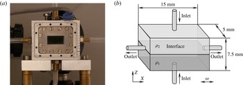
Experimental cell. (a) Photo of the cell, (b) Sketch of the inner part of the cell.

What concerns miscible fluids, the only known vibrational experiment was conducted by Legendre, Petitjeans & Kurowski (Reference Legendre, Petitjeans and Kurowski2003) with fluids of viscosity contrast
 ${\it\mu}_{2}/{\it\mu}_{1}=1000$
. The lack of experiments with miscible fluids is associated with severe experimental difficulties in forming a sharp interface, especially for fluids with similar viscosities. Furthermore, the system of two superimposed liquids has to be newly created after each experimental test. In the present work, we have designed and developed a dedicated set-up which allows us to create a sharp interface between two liquids miscible in any proportions. The interface is considered in a thermodynamic sense. Initially, the liquid–liquid system is assumed to be out of its thermodynamic equilibrium, and, in the absence of vibrations, its equilibration is driven by the diffusion process. During the reviewing process, further research studying the influence of the bounding walls (Shevtsova et al.
Reference Shevtsova, Gaponenko, Yasnou, Mialdun and Nepomnyashchy2015b
) and gravity (Gaponenko et al.
Reference Gaponenko, Torregrosa, Yasnou, Mialdun and Shevtsova2015) on the instability of miscible liquids were published; they are complementary to the present study.
The present paper is organized as follows. The experimental facility used, experimental conditions, measurement procedures and post-processing analysis are introduced in § 2. The mathematical model for a miscible multiphase system is defined in § 3. In the same section, besides the nonlinear Navier–Stokes equations, we introduce an averaging approach which decomposes equations into two parts with different time scales. The evolution of a flow field is discussed in § 4 with the aim of understanding the mechanism of frozen wave formation. The supercritical behaviour of frozen waves and their decay are analysed in § 5. The stability threshold of miscible interfaces and the comparison of the results with different theoretical approaches are given in § 6. In the same section, we discuss the determination of interfacial tension from a vibrational experiment. Finally, § 7 presents the summary of the obtained results.
2. The experiment
In order to study interfacial instability between miscible fluids under horizontal vibrations, we have developed a new instrument. The core of the experiment is the test cell: a rectangular cavity of 7.5 mm
 $\times$
5.0 mm
 $\times$
15.0 mm shown in figure 1(a). It corresponds to the aspect ratio (the length to the height)
 ${\it\Gamma}=L/H=2$
. Two opposite side walls of the cell are transparent, made of quartz glass (Hellma). The four other walls are made of aluminium alloy; each wall has a 0.4 mm diameter round orifice drilled it the centre for filling or draining the cell. See the separate sketch of the experimental cell in figure 1(b).
In order to create a flat and sharp ‘interface’ between two miscible liquids in the cell a special filling system has been developed. Both liquids are injected into the cell simultaneously by two identical syringe pumps through the orifices in the bottom (a denser liquid) and top (a lighter liquid) walls. The quality and thickness of the interface depend on the injection flow rate. While a high injection flow rate deforms the interface, a slow filling of the cell produces a wide interface with a reduced density gradient in the vertical direction. After several tests, a flow rate equal to
 $0.80~\text{ml}~\text{min}^{-1}$
was chosen for the experiments. The operation of the syringe pumps is controlled by a computer. The excess of liquid leaves the cell through the orifices located in the endwalls. This injection system allows for the formation of a thin straight interface in the middle plane (the
 $X$
–
 $Y$
plane) of the cell, and a fast replacement of the mixed liquids.
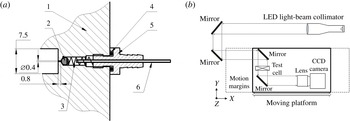
The cell is connected to the filling system and to the waste bag by using flexible tubes that allow us to maintain this connection during vibration. However, this kind of attachment may produce perturbations of the interface due to the bending of these tubes during the vibrations. In order to avoid this effect, four check valves made in-house (see figure 2 a) were installed into the cell to prevent a reverse flow. The cell is refilled with fresh fluids for each experiment to ensure a thin straight interface between the two miscible liquids.
The cell is fixed to a linear motor which performs translational oscillations in the
 $X$
direction at a controlled frequency and amplitude. In the experiments, the frequency and amplitude were varied within the ranges 2–24 Hz and 1.5–16 mm, respectively. The maximum vibrational acceleration of
 $8.4g$
was achieved at
 $A=4.3~\text{mm}$
and
 $f=22~\text{Hz}$
. The direction of the vibration is perpendicular to the concentration gradient and coincides with the initial horizontal interface.
The valve design and optical scheme of the experimental setup. Valve design: 1 – body of the cell made of aluminium alloy, 2 – steel ball of diameter 2.3 mm, 3 – spring, 4 – O-ring, 5 – fitting, 6 – steel capillary, soldered inside the fitting. (a) Valve design, (b) optical scheme.

The flow dynamics was monitored from the side by direct shadowgraphy of the interface. The optical scheme is illustrated in figure 2(b). The optical system used a collimated light generated by a LED source and a set of lenses. A set of mirrors was used to direct the beam path towards the moving platform. The collimated light beam traversed the test cell, and was then collected by the camera lens. The camera was fixed on the linear motor. Each data set consisted of 600 images taken at 48 f.p.s. and covering 12.5 s in time. To support the acquisition of full megapixel frames at this speed, all the frames were first grabbed into the volatile memory of the PC controlling the experiment, and then dumped into a single binary file on the hard drive of the PC. The binary file was then sliced by custom-made software into individual 10 bit greyscale frames of
 $1004\times 1004$
pixels size. These frames hold instantaneous snapshots of the interface state (with an exposure time of
 $200~{\rm\mu}\text{s}$
each) at a resolution of
 $57~\text{pixels}~\text{mm}^{-1}$
. The deviation of the light path due to the high density gradient results in images with dark regions corresponding to the interface.
The physical properties of the mixtures 90 % water–10 % IPA and 50 % water–50 % IPA (mass fraction) at
 $25\,^{\circ }\text{C}$
: density
 ${\it\rho}$
, kinematic viscosity
 ${\it\nu}$
, thermal diffusivity
 ${\it\chi}$
, diffusion coefficient
 $D$
and the Schmidt number
 $Sc={\it\nu}/D$
, characteristic viscous (
 ${\it\tau}_{vis}=H^{2}/{\it\nu}$
) and diffusion (
 ${\it\tau}_{D}=H^{2}/D$
) times when
 $H=0.00375~\text{m}$
.

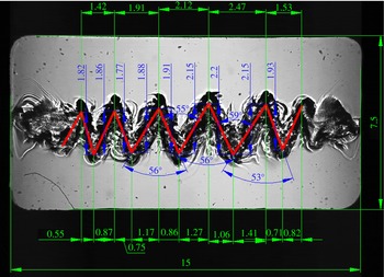
An example of image processing using CAD design software when
 $f=12.0~\text{Hz}$
,
 $A=11.8~\text{mm}$
.

The fluids used were 90 % (mass) of water in isopropanol and 50 % (mass) of water in isopropanol. The concentrations of the liquids were chosen for their well-known properties due to the experience of handling them (Mazzoni et al.
Reference Mazzoni, Shevtsova, Mialdun, Melnikov, Gaponenko, Lyubimova and Saghir2010; Shevtsova et al.
Reference Shevtsova, Lyubimova, Saghir, Melnikov, Gaponenko, Sechenyh, Legros and Mialdun2011). The parameters of the mixtures are presented in table 1. The solutions were degassed to avoid the presence of air bubbles. The density and viscosity contrasts between the two fluids were
 ${\it\rho}={\it\rho}_{2}/{\it\rho}_{1}=0.92$
,
 ${\it\nu}={\it\nu}_{2}/{\it\nu}_{1}=2.35$
or
 ${\it\mu}_{2}/{\it\mu}_{1}=2.17$
. All experiments were conducted at room temperature.
The recorded images of interest were processed using CAD design software; a typical example is shown in figure 3. All the quantitative results and plots below were produced on the basis of these measurements.
3. Mathematical formulation
We consider two superposed layers of incompressible and miscible liquids placed in a rectangular container, see geometry in figure 1. The denser liquid is placed in the lower layer, so that the configuration is gravitationally stable. The lower liquid is less viscous than the upper liquid, corresponding to the physical properties listed in table 1. Both layers have the same thickness
 $H=3.75~\text{mm}$
. The liquids are solutions of alcohol (isopropanol or IPA) in water of different concentrations, 0.90 water (liquid 1) and 0.50 water (liquid 2) in mass fraction, and they are miscible in all proportions. When the mixtures are brought into contact, the molecules of the neighbouring phases interdiffuse. In freshly created layers, the so-called Korteweg stresses due to concentration (density) difference may result in a small ‘effective’ interfacial tension which diminishes with time. Usually, even its initial value is two or three orders of magnitude smaller than that for typical immiscible liquids (Vorobev Reference Vorobev2014) and we do not take into account interfacial tension in the mathematical model.
Let us consider the mass fraction of the heavier liquid, water, as an independent variable (
 $\tilde{c}$
), then the initial concentration of liquid 1 is
 $\tilde{c}_{1}^{o}=0.90$
and liquid 2 is
 $\tilde{c}_{2}^{o}=0.50$
and
 ${\rm\Delta}\tilde{c}=(\tilde{c}_{1}^{o}-\tilde{c}_{2}^{o})$
. Furthermore, let us introduce the relative concentration of water to describe both layers with single independent concentration
 $C$
 $$\begin{eqnarray}C=(\tilde{c}-\tilde{c}_{2}^{o})/{\rm\Delta}\tilde{c},\quad 0\leqslant C\leqslant 1.\end{eqnarray}$$
Then the initial concentrations of the liquids are:
 $C^{o}=1$
in the lower layer and
 $C^{o}=0$
in the upper layer. Due to large concentration gradients at interfaces, density dependence on concentration cannot be disregarded. The dependence of the liquid density
 $\tilde{{\it\rho}}$
on the concentration
 $c$
is defined by a simple linearized relation valid for almost all liquid/liquid interfaces due to a small density contrast (i.e.
 ${\it\rho}_{2}/{\it\rho}_{1}=0.92$
).
 $$\begin{eqnarray}{\it\rho}={\it\rho}_{2}(1-{\it\beta}_{c}C),\quad {\it\beta}_{c}=({\it\rho}_{2}-{\it\rho}_{1})/{\it\rho}_{2}=-0.087.\end{eqnarray}$$
The mixture viscosity is a function of concentration with a maximum at
 $\tilde{c}^{o}=0.5$
(Mialdun et al.
Reference Mialdun, Yasnou, Shevtsova, Königer, Köhler, Alonso de Mezquia and Bou-Ali2012). In the region of interest,
 $0.5\leqslant \tilde{c}\leqslant 0.9,$
the viscosity can be approximated by a linear dependence.
 $$\begin{eqnarray}{\it\mu}(c)={\it\mu}_{2}(1-{\it\beta}_{{\it\mu}}C),\quad {\it\beta}_{{\it\mu}}=({\it\mu}_{2}-{\it\mu}_{1})/{\it\mu}_{2}=0.538.\end{eqnarray}$$
The origin of a Cartesian coordinate system is in the left lower corner of the cell and the
 $X$
-axis is parallel to the undeformed fluid interface. The
 $Z$
-axis is parallel to the Earth’s gravity, see figure 1(b). In the coordinate system associated with the cell, the acceleration applied to the system is the sum of gravitational and vibrational accelerations:
 $$\begin{eqnarray}\displaystyle \boldsymbol{g}+A{\it\omega}^{2}\cos ({\it\omega}t)\boldsymbol{e}, & & \displaystyle\end{eqnarray}$$
where
 $\boldsymbol{g}$
is the Earth’s gravity vector and
 $\boldsymbol{e}=(1,0,0)$
is the unit vector along the axis of vibrations.
3.1. Full nonlinear equations
For the current work we have adopted the Boussinesq approximation, its validity for the problem with vibrations was justified by Shevtsova et al. (Reference Shevtsova, Ryzhkov, Melnikov, Gaponenko and Mialdun2010). The system is considered isothermal. The equations of motion and mass transport are written
 $$\begin{eqnarray}\displaystyle \left.\begin{array}{@{}c@{}}\displaystyle \partial _{t}\boldsymbol{V}+(\boldsymbol{V}\boldsymbol{\cdot }\boldsymbol{{\rm\nabla}})\boldsymbol{V}=-\frac{1}{{\it\rho}_{2}}\boldsymbol{{\rm\nabla}}P+\frac{{\it\mu}_{2}}{{\it\rho}_{2}}\boldsymbol{{\rm\nabla}}((1-{\it\beta}_{{\it\mu}}C)\boldsymbol{{\rm\nabla}}\boldsymbol{V})-{\it\beta}_{C}C(\boldsymbol{g}+A{\it\omega}^{2}\cos ({\it\omega}t)\boldsymbol{e}),\\ \displaystyle \partial _{t}C+\boldsymbol{V}\boldsymbol{\cdot }\boldsymbol{{\rm\nabla}}C=D{\rm\nabla}^{2}C,\\ \displaystyle \boldsymbol{{\rm\nabla}}\boldsymbol{\cdot }\boldsymbol{V}=0.\end{array}\right\}\quad & & \displaystyle\end{eqnarray}$$
Here
 $\boldsymbol{V}$
is the velocity vector. The cell boundaries are rigid with a no-slip condition for the velocity and non-permeable for the concentration:
 $$\begin{eqnarray}\displaystyle \boldsymbol{V}=0;\quad \partial C/\partial n=0. & & \displaystyle\end{eqnarray}$$
The initial condition for velocity:
 $\boldsymbol{V}=0$
.
To be in better agreement with the experiment, three different types of the initial profile of the interface were tested:
 $$\begin{eqnarray}\displaystyle & & \displaystyle \text{(1) Sharp interface: }\nonumber\\ \displaystyle & & \displaystyle \qquad \qquad \qquad \qquad \qquad C=\left\{\begin{array}{@{}ll@{}}1 & \text{for }0<Z\leqslant H/2;\\ 0 & \text{for }H/2<Z\leqslant 1.\end{array}\right.\end{eqnarray}$$
 $$\begin{eqnarray}\displaystyle & & \displaystyle \text{(2) Diffusive interface: we allow the contact line to diffuse either 30 s or 60 s}\nonumber\\ \displaystyle & & \displaystyle \qquad \text{and consider the resulting concentration profile as initial.}\end{eqnarray}$$
 $$\begin{eqnarray}\displaystyle & & \displaystyle \text{(3) Linear transition inside the region }2{\it\delta}=0.45~\text{mm:}\nonumber\\ \displaystyle & & \displaystyle \qquad \qquad \qquad C=\left\{\begin{array}{@{}ll@{}}2(Z-{\it\delta})/H, & \text{for }H/2-{\it\delta}<Z<H/2+{\it\delta}\quad \text{and}\\ 1 & \text{for }0<Z\leqslant H/2-{\it\delta};\\ 0 & \text{for }H/2+{\it\delta}<Z\leqslant 1.\end{array}\right.\end{eqnarray}$$
3.2. Averaging approach
In addition to the calculations of full Navier–Stokes equations, a two-time-scale computational methodology was used for situations in which the forcing period is very small compared to the natural time scales of the problem. Let us denote the period of vibration by
 ${\it\tau}=1/f$
. In the averaging method (Gershuni & Lyubimov Reference Gershuni and Lyubimov1998), each field is decomposed into a ‘slow’ time-averaged part (with a characteristic time much longer than
 ${\it\tau}$
) and a ‘fast’ oscillatory part (with a characteristic time
 ${\it\tau}$
):
 $$\begin{eqnarray}\boldsymbol{V}=\overline{\boldsymbol{V}}+\boldsymbol{V}^{\prime },\quad C=\overline{C}+C^{\prime },\quad \widetilde{P}=\overline{P}+P^{\prime }.\end{eqnarray}$$
The time-averaged (mean) velocity and concentration are defined by
 $$\begin{eqnarray}\overline{\boldsymbol{V}}(t)=\frac{1}{{\it\tau}}\int _{t-{\it\tau}/2}^{t+{\it\tau}/2}\boldsymbol{V}({\it\tau}^{\prime })\,\text{d}{\it\tau}^{\prime },\quad \overline{C}(t)=\frac{1}{{\it\tau}}\int _{t-{\it\tau}/2}^{t+{\it\tau}/2}c({\it\tau}^{\prime })\,\text{d}{\it\tau}^{\prime }.\end{eqnarray}$$
The averaging approach is valid under the assumption that the period of vibration is much smaller than the reference viscous and diffusion times:
 $$\begin{eqnarray}{\it\tau}\ll \text{min}(H^{2}/{\it\nu}_{i},H^{2}/D).\end{eqnarray}$$
Another assumption follows from the requirement that the displacement of fluid particles during one period of oscillation should be much smaller than the characteristic length scale. The amplitude of vibration satisfies the inequality
 $A\ll L/{\it\beta}_{C}{\rm\Delta}C.$
An additional requirement is that the observed system should have a constant amplitude over a few periods. The derivation of the equations for averaged fields can be found in Shevtsova et al. (Reference Shevtsova, Ryzhkov, Melnikov, Gaponenko and Mialdun2010, Reference Shevtsova, Gaponenko, Sechenyh, Melnikov, Lyubimova and Mialdun2015a
).
The numerical modelling in the averaging approach is limited to a 2-D study with the purpose of understanding the fluid dynamics observed in the experiments. We computed the full nonlinear equations in the 3-D case for a few experiments, and noted that the interfacial pattern is basically independent of the spanwise direction (see § 5.2). The averaged equations will be solved in terms of a stream function
 ${\it\psi}$
and vorticity
 ${\it\zeta}$
, which are defined by
 $$\begin{eqnarray}\displaystyle v_{x}=\partial {\it\psi}/\partial z,\quad v_{z}=-\partial {\it\psi}/\partial x,\quad {\it\zeta}=\partial v_{z}/\partial x-\partial v_{x}/\partial z. & & \displaystyle\end{eqnarray}$$
The problem is solved in dimensionless variables by taking the scales of length
 $H$
, time
 $H^{2}/{\it\nu}$
, velocity
 ${\it\nu}/H$
, pressure
 ${\it\rho}{\it\nu}^{2}/H^{2}$
and the initial concentration difference
 ${\rm\Delta}\tilde{c}$
introduced earlier in (3.1). In the averaging approach we consider the viscosity of both layers to be equal to the mean value. The problem in the averaging formulation was considered in our previous studies by Gaponenko & Shevtsova (Reference Gaponenko and Shevtsova2008, Reference Gaponenko and Shevtsova2010) where the derivation of the governing equations were described. We should mention that a new function
 ${\it\varphi}={\it\Phi}{\rm\Delta}\tilde{c}H$
results from the decomposition of the vector
 $\overline{C}\boldsymbol{e}$
into its solenoidal
 $\boldsymbol{W}$
and irrotational
 $\boldsymbol{{\rm\nabla}}{\it\Phi}$
parts:
 $$\begin{eqnarray}\overline{C}\boldsymbol{e}=\boldsymbol{W}+\boldsymbol{{\rm\nabla}}{\it\Phi},\quad \boldsymbol{{\rm\nabla}}\boldsymbol{\cdot }\boldsymbol{W}=0.\end{eqnarray}$$
The equations for the oscillatory (fast) flow can be found in the above mentioned references. Hereafter, only the final equations for mean fields are given.
 $$\begin{eqnarray}\displaystyle & \displaystyle \frac{\partial {\it\zeta}}{\partial t}+\frac{\partial {\it\psi}}{\partial z}\frac{\partial {\it\zeta}}{\partial x}-\frac{\partial {\it\psi}}{\partial x}\frac{\partial {\it\zeta}}{\partial z}={\rm\nabla}^{2}{\it\zeta}-\frac{Ra}{Sc}\frac{\partial c}{\partial z}+\frac{Gs}{Sc}\left(\frac{\partial \overline{C}}{\partial z}\frac{\partial ^{2}{\it\varphi}}{\partial x^{2}}-\frac{\partial \overline{C}}{\partial x}\frac{\partial ^{2}{\it\varphi}}{\partial x\partial z}\right) & \displaystyle\end{eqnarray}$$
 $$\begin{eqnarray}\displaystyle & \displaystyle \frac{\partial \overline{C}}{\partial t}+\frac{\partial {\it\psi}}{\partial z}\frac{\partial \overline{C}}{\partial x}-\frac{\partial {\it\psi}}{\partial x}\frac{\partial \overline{C}}{\partial z}=Sc^{-1}{\rm\nabla}^{2}\overline{C} & \displaystyle\end{eqnarray}$$
 $$\begin{eqnarray}\displaystyle {\rm\nabla}^{2}{\it\psi}=-{\it\zeta},\quad {\rm\nabla}^{2}{\it\varphi}=-\frac{\partial \overline{C}}{\partial x}. & & \displaystyle\end{eqnarray}$$
The boundary conditions can be written in the form:
 $$\begin{eqnarray}\displaystyle \left.\begin{array}{@{}c@{}}x=0,2:\quad {\it\psi}=\partial _{x}{\it\psi}=0,\quad \partial _{x}\overline{C}=0,\quad \partial _{x}{\it\varphi}=\overline{C};\\ z=0,1:\quad {\it\psi}=\partial _{z}{\it\psi}=0,\quad \partial _{z}\overline{C}=0,\quad \partial _{z}{\it\varphi}=0.\end{array}\right\} & & \displaystyle\end{eqnarray}$$
The initial conditions are (
 $\tilde{{\it\delta}}={\it\delta}/H$
)
 $$\begin{eqnarray}\displaystyle \left.\begin{array}{@{}c@{}}t=0:\quad {\it\psi}={\it\zeta}=0,\quad \partial _{x}\overline{C}=0,\quad \partial _{x}{\it\varphi}=\overline{C};\quad \partial _{z}{\it\varphi}=0;\\ \overline{C}=1,\quad \text{when }0\leqslant z<0.5-\tilde{{\it\delta}};\quad \overline{C}=0\quad \text{when }0.5+\tilde{{\it\delta}}<z\leqslant 1;\\ \overline{C}=z,\quad \text{when }0.5-\tilde{{\it\delta}}<z\leqslant 0.5+\tilde{{\it\delta}}.\end{array}\right\} & & \displaystyle\end{eqnarray}$$
The description of the numerical method and code validation may be found in in Gaponenko & Shevtsova (Reference Gaponenko and Shevtsova2008). The system includes the Schmidt number
 $Sc$
, the Rayleigh number
 $Ra$
and the Gershuni number
 $Gs$
:
 $$\begin{eqnarray}\displaystyle Sc=\frac{{\it\nu}}{D},\quad Ra=\frac{g{\it\beta}_{c}{\rm\Delta}\tilde{c}H^{3}}{{\it\nu}D},\quad Gs=\frac{(A{\it\omega}{\it\beta}_{C}{\rm\Delta}\tilde{c}H)^{2}}{2{\it\nu}D}. & & \displaystyle\end{eqnarray}$$
For comparison with data in the literature, the dimensionless angular frequency
 ${\it\Omega}$
is defined using the largest viscosity
 ${\it\Omega}={\it\omega}H^{2}/{\it\nu}_{2}.$
Requirement (3.12) means that the dimensionless frequency
 ${\it\Omega}$
has to be large,
 ${\it\Omega}\gg 1.$
In the experiments, the dimensionless frequency
 ${\it\Omega}$
ranges between 45 and 545.
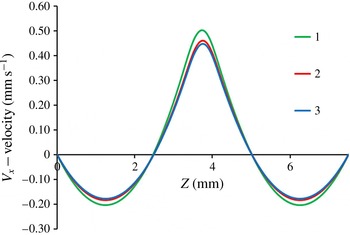
Resolution of the
 $V_{x}$
velocity along the vertical line at
 $X=4.5~\text{mm}$
on different meshes. Curves 1–3 correspond to
 $201^{x}\times 101^{z}$
,
 $401^{x}\times 201^{z}$
and
 $601^{x}\times 301^{z}$
, respectively.

Mesh convergence test for averaged equations.

3.3. Convergence of the numerical solutions
In order to study convergence of the numerical solutions, a set of calculations has been performed for full nonlinear and averaged equations using the following parameters of vibrations:
 $A=11.2~\text{mm}$
and
 $f=10~\text{Hz}$
. The computations have been performed on uniform grids with a number of points
 $N^{x}\times N^{z}$
.
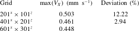
Averaging approach. The convergence of the numerical solutions has been examined for three different meshes. The profiles of the horizontal velocity along the vertical line were selected for analysis at
 $X=4.5~\text{mm}$
, because the centres of a four-vortex flow structure are located at this plane. Table 2 and figure 4 show the convergence of the numerical solution upon mesh refinement at the time
 $t=0.71~\text{s}$
. Due to the small relative difference in peak values of the velocity between
 $601^{x}\times 301^{z}$
and
 $401^{x}\times 201^{z}$
(2.94 %), the latter mesh was chosen for further simulations.
Resolution of the vertical (a) and horizontal (b) velocities at
 $Z=3.75~\text{mm}$
on different meshes. Curves 1–3 correspond to
 $241^{x}\times 121^{z}$
,
 $401^{x}\times 201^{z}$
and
 $801^{x}\times 401^{z}$
, respectively.

Mesh convergence test for full equations.

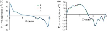
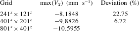
Full nonlinear equations. The flow pattern consists of one big vortex centred in the middle of the cell which changes its direction each half-period; as can be seen in figure 5(a). To obtain mean flows, the computed quantities are summed over a few oscillation cycles, and then divided by the number of time steps. The full flow is much stronger in comparison with the averaged flow. The profiles of the horizontal and vertical velocities of the full flow obtained on different meshes are shown in figure 5 for
 $Z=3.75~\text{mm}$
at time
 $t=0.525~\text{s}$
. The parameters for the meshes are shown in table 3. The profiles of the vertical velocity along the cell demonstrate a good agreement on all three meshes, the maximal difference between the peak values is less than 5 %. To look more accurately at the convergence of the solution, the profile of the horizontal velocity is shown in the same figure on the right-hand side. This panel characterizes the finer structures inside a big vortex and somewhat closer corresponds to the averaged flow which is responsible for instability in the considered system. The difference in resolution between the meshes becomes noticeable only in the points of inflection of the
 $V_{x}$
-velocity profile. According to the results of the comparison given in table 3 at the point
 $X=14~\text{mm}$
,
 $Z=3.75~\text{mm}$
, the spatial mesh
 $401^{x}\times 201^{z}$
is selected for the simulations. Obtaining well-resolved vibrational boundary layers is vital. The thickness of vibrational viscous boundary layers in the experimental parameter space varies within the ranges
 $$\begin{eqnarray}\displaystyle {\it\delta}_{1}=\sqrt{2{\it\nu}_{1}/{\it\omega}}=0.22{-}0.33~\text{mm},\quad {\it\delta}_{2}=\sqrt{2{\it\nu}_{2}/{\it\omega}}=0.14{-}0.21~\text{mm}, & & \displaystyle\end{eqnarray}$$
Thus, at least four grid points were used in the thinnest boundary layer.
The time step size was selected so that it is always smaller than the viscous, diffusion time scales and the period of the vibrations, i.e.
 ${\rm\Delta}t<\min (H^{2}/{\it\nu}_{2};H^{2}/D;1/f)$
. In all the cases presented in this work, the oscillation period
 $O(10^{-2}~\text{s})$
is the leading criterion, which is logical given that the largest frequency in the experiments was 24 Hz and about 10 points per period are desirable. This leads to a time step of
 $10^{-3}~\text{s}$
, which is very small with respect to all of the characteristic time scales. However, to satisfy the low Courant number criterion at small spatial steps (
 ${\rm\Delta}x,{\rm\Delta}z$
), the time step was reduced to
 ${\rm\Delta}t\sim 10^{-4}~\text{s}$
.
4. Evolution of flow field and formation of frozen waves
Below the threshold of instability two different flow patterns were observed. In the experiments with low frequencies (
 $f=2~\text{Hz}$
) and large amplitude (
 $A\geqslant 5~\text{mm}$
) sloshing flow was excited. In the case of high frequencies (
 $f>20~\text{Hz}$
) and smaller amplitude (
 $A\leqslant H$
) a wavy pattern either was not formed at all or quickly damped out, replaced by a straight contact line. At the threshold of an interfacial instability, a pair of surface waves emerged, which travel along the contact line from the lateral walls inwards. One should consider the time interval between the waves that are created at the endwalls of the cell, and appear at the centre of the cell. The amplitude of the wave is decreased by viscous dissipation as it travels. The first interaction of the wave train created at the opposite endwalls corresponds to a destructive interference. Thus, there is a threshold time
 $t_{0}$
for instability to set in after imposing vibrations. The onset time
 $t_{0}$
depends on the vibrational forcing and the sharpness of the interface.
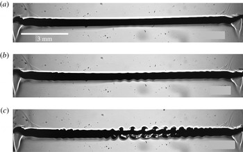
Spatio-temporal evolution of the interface near the threshold of instability at successive times (vertical axis is not in scale). The experimental parameters are
 $f=22~\text{Hz}$
,
 $A=3~\text{mm}$
,
 $g_{os}/g=6.9$
,
 ${\it\Omega}=500$
: (a)
 $t=6$
s; (b)
 $t=8$
s; (c)
 $t=10$
s.

4.1. Dynamics of an interface near the onset of instability
Here we consider the dynamics of an interface using the example of a high frequency, 22 Hz, and an amplitude comparable to the height of one layer,
 $A=3~\text{mm}$
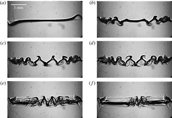
. Figure 6 shows the temporal-spatial evolution of the surface waves (concentration gradient) at the onset of instability. The positions of the interface are magnified. The snapshots are selected at nearly the same phase of oscillations. The image at
 $t=6~\text{s}$
in figure 6 reveals that tiny amplitude interfacial waves propagate from the lateral walls inwards and decay. Later in time, in the snapshot at
 $t=8~\text{s}$
, the wavy pattern reveals an interesting structure, when the amplitude of the surface waves essentially vary along the contact line. At time
 $t=10~\text{s}$
, the waves with a modulated amplitude cover almost the entire interface. It is worth highlighting that it is the first experimental evidence of spatially modulated waves on an interface caused by horizontal vibrations. Previous experimental studies of wave patterns under horizontal vibrations with immiscible fluids (Jalikop & Juel Reference Jalikop and Juel2009; Yoshikawa & Wesfreid Reference Yoshikawa and Wesfreid2011b
; Gandikota et al.
Reference Gandikota, Chatain, Amiroudine, Lyubimova and Beysens2014b
) did not report wave modulation, although it was theoretically predicted by Varas & Vega (Reference Varas and Vega2007) in a nearly inviscid fluid subjected to horizontal vibration. We will return to this pattern in § 4.3.
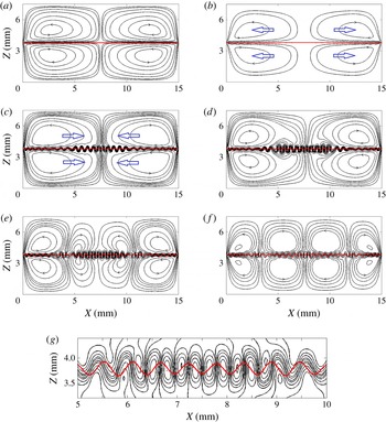
(Computer simulations of the averaged equations.) The spatio-temporal evolution of the instability at the threshold. The isolines of the stream function (for mean flow
 $\overline{\boldsymbol{V}}(X,Z)$
) and the interface shape (mean concentration
 $\overline{C}(X,Z)$
) in different dynamic regimes. In order to highlight the active regions, 14 non-equidistant isolines (denser around zero) are depicted between the minimum (
 $-0.02$
) and maximum (0.02) in graphs (a,b) and for graphs (c,d) the levels are smaller: 16 isolines between the minimum (
 $-0.003$
) and maximum (0.003). The interface is shown by three isoconcentration levels 0.5,
 $0.5\pm 0.001$
. Other parameters are
 $f=22~\text{Hz}$
,
 $A=3~\text{mm}$
. (a) regime I,
 $t=1.6$
s; (b) regime Ia,
 $t=9$
s; (c) regime II,
 $t=15.6$
s; (d) regime III,
 $t=17.0$
s; (e) regime III,
 $t=18$
s; (f) regime III,
 $t=20.0$
s; (g) magnified interfacial region from graph (e) at
 $t=18$
s.

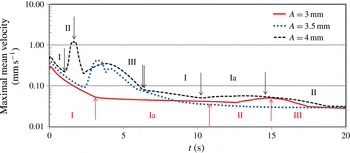
(Numerical results of the averaged equations in a logarithmic scale.) Temporal evolution of the maximal velocity of the mean flow
 $\overline{\boldsymbol{V}}(X,Z)$
for the frequency,
 $f=22~\text{Hz}$
, and different amplitudes
 $A=3.0~\text{mm}$
(solid curve),
 $A=3.5~\text{mm}$
(dotted curve) and
 $A=4.0~\text{mm}$
(dashed curve). For clarity the vertical arrows outline the change of flow dynamics regimes only for two amplitudes,
 $A=3~\text{mm}$
and
 $A=4\;\text{mm}$
.

4.2. Dynamics of a mean flow near the onset of instability
Vibrations produce deformations of the interface as well as an oscillatory flow in the bulk and mean flows. Viscous mean flows are proved (Higuera, Vega & Knobloch Reference Higuera, Vega and Knobloch2002) to couple dynamically with the evolution of the surface waves. To understand the experimentally observed scenario of instability, we resort to the analysis of the mean flow at the onset. To gain insight into the development of instability in time, the problem was solved numerically in the averaged formulation, i.e. (3.10)–(3.12). The initial interface profile was assumed to be linear, (3.19). The spatio-temporal dynamics of flow patterns can be subdivided in three intermediate regimes which are repeated over time. For the discussion below, the two figures, figures 7 and 8, will be used simultaneously.
I. Formation of a mean flow pattern symmetric to the contact line. Since vibrations are imposed, small vortices are formed on each side of the diffusive interface adjacent to the endwalls. Progressively their cores move toward the cell centre fluctuating upward and downward in time until they align along the interface. For the considered case,
 $f=22~\text{Hz}$
and
 $A=3~\text{mm}$
, the streamlines of the mean flow at the end of this regime (
 $t=1.6~\text{s}$
) are shown in figure 7(a) where the red horizontal curve outlines the contact line between liquids presented as a few isolines of the mean concentration
 $\overline{C}$
. At the end of this step, only tiny disturbances of the interface set in near the lateral walls (they are not visible in the scale of the figure). During this regime, the maximal velocity of the mean flow
 $\overline{\boldsymbol{V}}(X,Z)$
significantly diminishes (see the solid curve in figure 8 presented in a logarithmic scale).
Ia. Vortices recurrence (only for weak flows at the onset of instability). As time goes by, the vortex cores start moving back toward the endwalls. The diffusive interface in the middle is slightly thinning during the horizontal displacement of vortices along the contact line. Over this time interval, the maximal velocity of the mean flow in figure 8 changes very slowly. At the end of this step,
 $t\approx 9~\text{s}$
, the interface perturbations start growing locally: stronger near the walls and weaker at the central part. The stream functions of the mean flow and the interface shape are shown in figure 7(b). The levels of isolines in panels (a,b) are equal. It is important to note that this regime is observed only when the mean velocity is small; either at the onset of instability or in a supercritical state in the second cycle of regime changes. For example, compare the location of this regime in time for the solid (threshold) and dashed (supercriticality) curves in figure 8.
II. Formation of a wavy interfacial pattern. One of the key features of this regime is the formation of interfacial waves. Figure 7(c) highlights the waviness of the stream functions near the contact line and the resulting interface profile (red curve) at
 $t=15.6~\text{s}$
. The flow pattern consists of four large symmetric vortices with the same direction of the cores displacement as in regime I in panel (a) but with a wavy interface. Note, that the levels of the isolines in panel (c) are smaller than in panels (a,b). The subsequent evolution is the following; the cores of the vortices start again to move from the lateral walls inwards. The velocity of the mean flow (figure 8) grows and reaches a local maximum before decaying at large times. Growing deformations, extending from the endwalls, occupy the entire line of contact between the fluids. In agreement with experimental observations, the amplitude of the generated interfacial waves is spatially modulated. The smallest amplitude (height) is observed at the contact point between the two counter-rotating vortices. The time interval for the existence of this regime is indicated in figure 8.
III. Reorganization of vortices. This regime is characterized by a strong vortical activity. The vortices spreading from the opposite sides come into contact and start to break into several big and many smaller ones, see snapshots in figure 7(d–f). The number of large intermediate vortices depends on the vibrational forcing and the time instant. Each interfacial wave is generated by two small vortices, as seen in the magnified picture of the central part of the interface in figure 7(g) at
 $t=18~\text{s}$
. The waves on the interface are stabilized during this step although their wavelength is still affected by the flow dynamics. The dynamical transitions continue until a temporally stable pattern with four big vortices in each layer is formed, as shown in figure 7(f) at
 $t=20~\text{s}$
. The pairs of central vortices have a similar strength but they are weaker than the ones at the walls. The crests and troughs do not change their position with time in the horizontal direction in a reference frame associated with the cell. Hence, one can speak about frozen waves. Figure 7(f) also demonstrates spatial amplitude modulation, which can be seen as two depletion zones in the interfacial wavy pattern at
 $X=4~\text{mm}$
and
 $X=11~\text{mm}$
. It occurs on the border between strong and weak counter-rotating vortices. After that, the flow remains transient, but its velocity is too small to change noticeably the established wavy pattern. At a later time, the shape of the waves is gradually modified by convective mixing and diffusion.
4.3. Comparison of the experimental and numerical observations near the threshold
The regimes described above provide insight into the mean flow evolution and they are perfectly supported by the experimental findings in figure 6. The snapshot at
 $t=8~\text{s}$
shows the formation of interfacial waves according to regime II, when the cores of the vortices move inwards after retreat. All the images undoubtedly demonstrate the spatial modulation of the interfacial waves predicted by the evolution of the mean flow. Furthermore, the snapshots at
 $t=10~\text{s}$
confirm the predicted wavy pattern in regime II that the maximal amplitude is attained in the central part but the waviness contains the depletion zones on both sides from the centre, see snapshots in figure 7(d–f). After saturation, the interfacial pattern, the so-called frozen waves, remains unchanged for a relatively long time.
Although there is a perfect agreement in flow dynamics between the computer simulations of the mean flows and the experiments, the threshold time of the instability
 $t_{0}$
is different. The difference can be attributed to the initial interface profile and usual non-ideality of the experiment. Another point is that the tips of the crest are sharp in figure 7 while they are smeared at the experiments. To obtain the smearing of the tips, full Navier–Stokes equations should be solved instead of time-averaged equations (see figure 12 and further discussion).
4.4. Flow evolution with the increase of the amplitude of vibrations
Here we examine the effect of the amplitude of vibrational forcing on the strength of the mean flow and its dynamics. Figure 8 compares the temporal behaviour of the maximal velocity for three different amplitudes (3.0, 3.5 and 4.0 mm) at a given frequency
 $f=22~\text{Hz}$
, consequently, each velocity profile corresponds to different distances from the critical point. The results demonstrate that the succession of the dynamic states are similar for all the amplitudes. However, with the increase of the amplitude their evolution occurs in an accelerated and more powerful manner. The peak velocities strongly differ for the three curves. Note that the velocity in figure 8 is shown in a logarithmic scale. The vertical arrows separate regimes described in § 4.2 and facilitate understanding the evolution of the patterns. The flow dynamics at the critical amplitude, i.e.
 $A=3~\text{mm}$
, (the solid red curve) was discussed in detail in § 4.2. It is worth recalling that the waves on the interface started to form at the beginning of regime II,
 $t\approx 11~\text{s}$
. At strong forcing, the first regime is transformed directly into the second one without vortex recurrence in intermediate regime Ia. For the amplitude
 $A=3.5~\text{mm}$
(the dotted blue curve), the waviness starts to cover the initially planar contact line much earlier (
 $t=2.3~\text{s}$
), at the time of the first local minimum of the velocity. For a better visibility of the general trends in figure 8, the arrows are not indicated for this case. At a larger amplitude,
 $A=4~\text{mm}$
(the dashed curve in figure 8), it occurs even earlier (
 $t=1.35~\text{s}$
), but again, a wave starts to develop at the time of the first local minimum. The succession of local extrema reflects the transformation of large vortices.
An important observation is that after the first cycle, the three distinct flow regimes are repeated. However the driving force, a density difference across the interface, is weaker in the following cycle and the flow velocity is much smaller.
4.5. Flow dynamics via trajectories of particles
High-frequency vibrations with a small amplitude generate in bulk both an oscillatory (fast) and a mean (slow) flow which can be separated, see (3.10) in § 3.2. When particles in fluid are subjected to a high-frequency vibrational field, their trajectories also can be seen as ‘fast’ and ‘slow’ motions. Light small particles are moving with the flow field, although they may not follow exactly the fluid streamlines as their inertia slightly influences the trajectories.
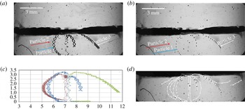
Trajectory of particles advected by a fluid flow. Experimental parameters:
 $f=22~\text{Hz}$
,
 $A=3.5~\text{mm}$
,
 ${\it\Omega}=500$
. (a) Image made with 500 superimposed images, keeping minimum pixel intensity for each pixel. (b) Image made with 1 out of every 11 images, keeping minimum pixel intensity for each pixel. (c) Trajectories of three particles tracing slow and fast flows in the bottom layer. (d) Mean flow tracing in the bottom layer.

A few small particles of polytetrafluoroethylene or teflon (PTFE), possibly sitting on the wall of tubing, appeared in the cell during several experiments. With a characteristic diameter of particles
 $D_{p}$
between 20 and
 $80~{\rm\mu}\text{m}$
, an estimated particle Stokes number (St) for the experiments discussed below is
 $$\begin{eqnarray}St=\frac{{\it\rho}_{p}}{{\it\rho}_{1}}\frac{D_{p}^{2}U_{ch}}{18{\it\nu}_{1}H}\approx (5{-}10)\times 10^{-3}\ll 1\end{eqnarray}$$
here the density of particles is assumed to be equal to the density of the liquid and the characteristic flow velocity is the peak vibrational velocity
 $U_{ch}=A\cdot {\it\omega}$
. Such light small particles are expected to move with the flow field.
The particle trajectory images shown in figures 9(a,b) in the experiment with
 $f=22~\text{Hz}$
,
 $A=3.5~\text{mm}$
, were obtained by superimposing consecutive images while keeping a minimum intensity for each pixel. Figure 9(a) includes 500 out of 600 acquired images and shows the trajectories of all the available particles. For better understanding, the trajectories of three distinctive particles are presented in figure 9(c). The small-amplitude oscillations, as well as average displacement of the particles, can be observed. A fast oscillating contribution seen in the horizontal
 $X$
coordinate, that has the same frequency as the imposed external vibration, is superimposed on a mean flow with a slow characteristic time scale. Consider that the image acquisition rate of 48 images per second is barely twice the vibration rate of
 $f=22~\text{Hz}$
, there is some aliasing effect on the sampled high-frequency trajectory.
The evolution of the mean flow without high-frequency contribution could be observed while selecting images at the same phase of the vibration period. As the camera acquisition rate (48 f.p.s.) is not, for the case with detected particles, an integer multiple of the imposed vibration frequency (22 Hz), it is not possible to show images taken at the same phase per period. But we can follow the mean flow by tracking particle positions showing each eleventh consecutive image, which corresponds to nearly 1 image per 5 vibrations, as they will be almost at the same phase (0.229 s, 5.04 s periods). To do so, in figures 9(b,d) only each eleventh consecutive image is superimposed while keeping a minimum intensity count for each pixel. The ensemble of particles represents directly the mean flow without fast oscillations. The arrows in figure 9(d) highlight the features of the mean flow, clearly demonstrating a flow pattern with two vortices near the cell centre.
Let us compare the numerical predictions of the mean flow with those recovered by means of particle tracing. The resulting trajectories outline the full time history of the transient flow, while the isolines in figure 7 present different regimes of the mean flow at selected time instants. The computed time history of the mean flow for this set of parameters can be seen as the evolution of the maximal velocity shown by the dotted line in figure 8. Indeed, the particle observation begins to be possible from the moment when the velocity starts to grow and lifts the particles (from the 100th image or from
 $t=2~\text{s}$
in figure 8). In the course of time, the trajectories of particles 1 and 2 in figure 9 experimentally confirm the flow dynamics predicted numerically in III regime (outlined in figure 7), when a flow pattern contains two vortices rather steady in time near the cell centre. The trajectory of particle 3 can be understood as it was trapped between counter rotating vortices (central and lateral) which change size and position in time; this dynamics can be traced quite clearly in panels (d–f) in figure 7. The excellent agreement between the computed and the experimental dynamics indicates that the evolution of the mean flow accurately predicts the temporal development of the interfacial instability.
4.6. Shear between miscible liquids
One may get a first impression from figure 7 that the flows in both layers are symmetrical and shear is absent. However, as discussed in the introduction, the interfacial wavy pattern between immiscible liquids under horizontal vibrations was associated to the Kelvin–Helmholtz instability. Since the densities of both liquids are different, one of them is accelerated faster and in a closed cell, this results in a horizontal pressure gradient that induces oscillatory shear flows. The flow becomes unstable when the relative velocity of the layers is larger than a critical value.
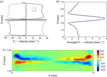
The computed flow for the parameters above the onset of the frozen waves at
 $t_{0}=0.8~\text{s}$
for
 $f=8~\text{Hz}$
,
 $A=12~\text{mm}$
. (a) The snapshots of full axial velocity
 $V_{X}$
across the cell at
 $t_{0}$
(curve 1) and
 $t_{0}+1/(2f)$
(curve 2) in the cell centre,
 $X=L/2$
; the shadow outlines a miscible interface. (b) The axial velocity
 $\overline{V}_{X}$
averaged over two subsequent periods of oscillations at
 $X=0.15L$
. (c) The distribution of the mean shear stress
 ${\it\mu}\,\text{d}U_{X}/\text{d}z$
(only the central part of the cell height is shown); the shear is averaged over two periods of oscillations.

The visible symmetry in figure 7 is due to the fact that the averaged (streaming-like) flows are weak; they are one order of magnitude smaller than full flows, i.e.
 $O(1/f)$
. In addition, the flows were shown near the threshold where the mean flows and shear are still small. To obtain a more representative sample of shear in the miscible problem, we selected vibrational parameters above the threshold of instability. Figure 10 demonstrates that in the case of miscible liquids the differential acceleration of the two liquids also results in a counterflow that generates oscillatory interfacial shear. The two profiles of the full velocity in the horizontal direction are shown in panel (a) in the time instants shifted by one half of the period. The shaded region outlines the non-zero thickness of a miscible interface. The snapshots show axial velocity at the cell centre, where the mean flows are still small at this time interval. Figure 7(b) showed that the interface perturbations appear near the walls and the averaged flow and shear are stronger at those locations. Correspondingly, the averaged axial velocity in panel (b) is shown closer to the wall at
 $x=0.15L.$
The maximum value of the mean velocity near the contact line indicates a hydrodynamic pressure gradient in this region. The time-dependent calculations of (3.5)–(3.9) demonstrate that shear stress oscillates in time resulting in non-zero mean value. Panel (c) shows shear stress in the cell averaged over two periods. It clearly indicates a substantial shear near the walls, where the waves are already formed, and almost zero shear in the central part of the cell. Thus, figure 10 suggests that frozen waves in miscible liquids are caused by a shear-driven mechanism similar to the Kelvin–Helmholtz instability.
5. Supercritical regime
Experimentally observed spatio-temporal evolution of the interface in a supercritical regime. The experimental parameters are
 $A=11.2~\text{mm}$
,
 $f=10~\text{Hz}$
,
 $g_{os}/g=4.5$
,
 ${\it\Omega}=227$
. (a)
 $t=0.3$
s, (b)
 $t=1.16$
s, (c)
 $t=1.5$
s, (d)
 $t=2.16$
s, (e)
 $t=5.86$
s, (f)
 $t=10.66$
s.

5.1. Development and smearing of frozen waves
The experiments examined in this section differ from the ones in § 4 in two ways; (a) the amplitude of vibrations is large (larger than the cell height
 $2H$
but smaller than the cell length
 $L$
); (b) the frequency is smaller. An interesting observation of flow dynamics in the supercritical regime was acquired in the experiment with
 $A=11.2~\text{mm}$
and
 $f=10~\text{Hz}$
. It resulted in smaller (by 1.5 times) vibrational acceleration
 $g_{os}/g$
with respect to figure 6. The succession of snapshots in figure 11 shows the behaviour of the interface at different times during the experiment. The images are nearly at the same phase, but the frequency
 $f=10~\text{Hz}$
is not a multiple value of the 48 f.p.s. of the CCD camera and a small inclination can be noticed from one image to another. The interfacial dynamics is similar to that described in § 4.2 for the case of high frequency and smaller amplitude. Indeed, the interface deformation at
 $t=1.16~\text{s}$
coordinates with the flow pattern at the beginning of regime II, when perturbations start to extend from the lateral walls.
With increasing time, we see the emergence of more and larger waves, and, soon, the waves cover the entire line of contact (
 $t=1.5~\text{s}$
) after which, the waves in the central part are frozen, although near the lateral walls, the wave pattern starts to decay (
 $t=2.16~\text{s}$
). Because of viscous dissipation, any initial perturbation will be damped out if there is no balance between driving force and dissipation. In miscible liquids, one of the principal restoring forces usually supporting short waves, the interfacial tension (in the sense of Korteweg stresses), vanishes with the decrease in the density gradient, and the wave amplitude attenuates. The interface dissipates a bit faster within a more viscous layer. At later times, the dense ripples near the wall extend to the centre from different sides and squeeze the wavy pattern (Shevtsova et al.
Reference Shevtsova, Gaponenko, Yasnou, Mialdun and Nepomnyashchy2015b
).
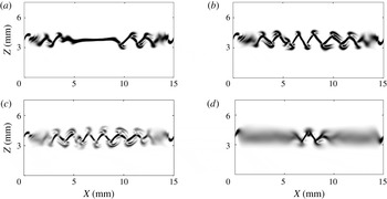
The concentration gradients computed from nonlinear Navier–Stokes equations (3.5)–(3.7) at different time instants. The parameters are the same as in the experiment shown in figure 11:
 $A=11.2~\text{mm}$
,
 $f=10~\text{Hz}$
. (a)
 $t=0.725~\text{s}$
, (b)
 $t=1.125~\text{s}$
, (c)
 $t=1.525~\text{s}$
, (d)
 $t=4.025~\text{s}$
.

We have analysed mean flows to elucidate the physical mechanisms of the emergence of frozen waves. The interfacial patterns in figure 11 are well explained by the dynamic regimes using calculations of the mean flows. It was stated in § 3 that the averaging approach is valid in the limit of high frequencies. Indeed, the dimensionless frequency
 ${\it\Omega}$
is large in both experiments presented in figure 6 (
 ${\it\Omega}=500$
) and in figure 11 (
 ${\it\Omega}=227$
). Furthermore, for the major part of our experiments, the evolution of the mean flow offers a clear explanation for instability development. It is noteworthy that, in the derivation of the averaged equations, the existence of the Stokes boundary layer for the oscillatory flow is not taken into account. Consequently, the simulation of the averaged equations cannot reveal the role of viscous dissipation near the walls. To better understand the attenuation of the instability from the endwalls, full nonlinear Navier–Stokes equations (3.5)–(3.7) were solved. The resulting numerical patterns in figure 12 are presented via the concentration gradient because our experimental technique is adjusted to provide gradients of density. All the distinctive characteristics of the experimental patterns in figure 11, such as formation of triangular shaped waves with duck tips and dissipation from the wall at later times, are numerically reproduced in the nonlinear simulations presented in figure 12.
5.2. Three-dimensional flow
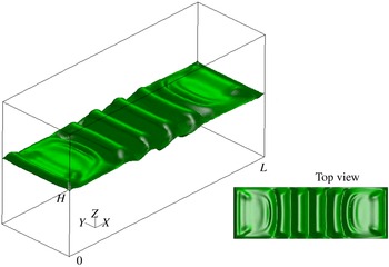
The results presented above demonstrate interfacial instability between two ordinary miscible liquids. However, it is still unclear to what extent 2-D simulations and side observation in the experiments describe correctly the full physical phenomenon. Here we investigate the interface behaviour by means of a 3-D simulation of nonlinear equations for
 $A=11.2~\text{mm}$
and
 $f=10~\text{Hz}$
. Figure 13 depicts a view of the surface with concentration
 $C=0.5$
while the small insertion shows the top view. We notice that the concentration pattern is essentially 2-D except in small near-wall regions in the direction perpendicular to the wave. These results illustrate that 2-D simulations reflect correctly the growth of the interfacial instability. Furthermore, the small 3-D effects near the sidewalls (
 $Y=0$
and
 $Y=5~\text{mm}$
) explain the origin of the extra perturbations of the wave shape near the crests and tips while observing from the side. In conjunction with the no-slip velocity boundary condition at the walls of the cell, the
 $C=0.5$
surface remains ‘anchored’ at its initial endwalls locations at
 $X=0$
and
 $X=L$
. The purpose of this study is to present a qualitative picture of the concentration pattern and 3-D calculations were performed on a rougher mesh than a 2-D one. Because of this, there is a difference between figures 12 and 13. The number of points in the
 $X,Y$
directions correspond to the first line in table 3 and the used mesh was
 $241^{x}\times 121^{z}\times 51^{y}$
.
A view of the surface with concentration
 $c=0.5$
at
 $t=1.325~\text{s}$
; the insertion shows top view. Simulation of the nonlinear 3-D equations are performed for
 $A=11.2~\text{mm}$
and
 $f=10~\text{Hz}$
.

5.3. Wave shape
One of the features that highlights the difference between immiscible and miscible fluids in the frozen wave instability is the wave shape. Since the time
 $t=1.5~\text{s}$
, the images in figure 11 show quite clearly that the waves are triangular in shape. The nonlinear simulations in figure 12 also show a saw-tooth shape which is in line with the experiments. Primarily, this is attributed to the vanishing surface energy. The vanishing interfacial tension makes the tips of the crests and troughs sharp. For immiscible fluids, this shape is known to be sinusoidal (Ivanova et al.
Reference Ivanova, Kozlov and Evesque2001; Talib et al.
Reference Talib, Jalikop and Juel2007).
The shape of the interface can be determined by the normal projection of the stress balance between liquids (the normal vector
 $\boldsymbol{n}$
directed into liquid 1)
 $$\begin{eqnarray}[P_{1}-P_{2}]-(\boldsymbol{n}S_{1}\boldsymbol{n}-\boldsymbol{n}S_{2}\boldsymbol{n})={\it\sigma}K.\end{eqnarray}$$
Here
 $\unicode[STIX]{x1D64E}={\it\mu}(\partial V_{i}/\partial x_{k}+\partial V_{k}/\partial x_{i})$
is the viscous stress tensor,
 $K$
is the curvature and
 $P$
is the pressure. Considering the interface as frozen, the viscous terms can be omitted. Then
 ${\rm\Delta}P\sim {\it\sigma}K$
and in the case of miscible liquids the vanishing interfacial tension
 ${\it\sigma}\rightarrow 0$
should be compensated by a very large curvature,
 $K\rightarrow \infty ,$
at the crests and troughs. This results in a sawtooth-like wave shape.
It was shown in § 4 that the mean flow is coupled with the interfacial waves. Figure 8 shows a repeating of the sequence of the mean flow regimes after the first cycle, but at a much lower intensity. This illustrates that ‘frozen’ waves are slightly moving, but these displacements are much smaller than the amplitude of the waves. These small displacements suggest that for a very large viscosity ratio, the viscous terms in (5.1) cannot be discarded completely. The authors of the only known experiment with miscible fluids (Legendre et al.
Reference Legendre, Petitjeans and Kurowski2003) observed a sine shape, however, the test fluids had a very large viscosity contrast,
 ${\it\nu}\sim 1000$
.
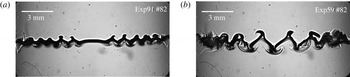
The interface pattern at the same time moment
 $t=1.7~\text{s}$
for different frequencies and amplitudes (a)
 $f=22.5~\text{Hz}$
,
 $A=3.6~\text{mm}$
; (b)
 $f=10~\text{Hz}$
,
 $A=11.2~\text{mm}$
.

The transformation of the wave shape was observed at a liquid–vapour interface in the experiments with near-critical hydrogen subjected to horizontal vibrations (Gandikota et al.
Reference Gandikota, Chatain, Amiroudine, Lyubimova and Beysens2014a
). They reported a sharp triangle shape far from the critical point and a somewhat rounded shape very close to the critical point and assigned this difference to the interplay between vibrational forcing and viscous dissipation. We may suggest that the shape rounding near the critical point was attributed to a lowering of the gravity level in their experiments because
 ${\rm\Delta}P$
in (5.1) includes hydrostatic pressure, see Gaponenko et al. (Reference Gaponenko, Torregrosa, Yasnou, Mialdun and Shevtsova2015).
5.4. Wave properties
Over the range of experimental runs we examined the formation and advancement of interfacial waves with time. In agreement with the comment by Gonzalez-Vinas & Salan (Reference Gonzalez-Vinas and Salan1994), we found the time delay
 $t_{0}$
before the instability sets in and the wavy pattern that can be observed is longer at higher frequencies. A comparison of the interface patterns for different frequencies and amplitudes is shown in figure 14 at
 $t=1.7~\text{s}$
. The observed wave dynamics shows that, after formation, the wave steadiness is weakly dependent on the forcing frequency. For the range of frequencies
 $f\geqslant 21~\text{Hz}$
the position of the crests and troughs of the central peaks remains constant during the observation time. In the case of smaller frequencies and larger amplitudes, the findings are different. Note that the latter frequencies still satisfy the limit of high frequencies (
 ${\it\Omega}\gg 1$
).
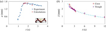
Figure 15(a) shows the temporal evolution of the wave height
 $a$
(crest-to-trough length) in the experiment with
 $A=11.2~\text{mm}$
and
 $f=10~\text{Hz}$
(
 ${\it\Omega}=227$
) from the time moment at which it was possible to determine it accurately. The data were extracted using the procedure presented in figure 3 with an uncertainty of approximately 5–10 % based on human error. From the beginning of the observation, the wave height of the central peaks grows with time. This quasi-linear amplification continues until the wave height reaches a maximum value
 $a=1.65~\text{mm}$
, which is approximately half of the layer thickness
 $a/H\approx 0.45$
. Then, the waves begin to relax to their final saturated state
 $a=1.48~\text{mm}$
, which is approximately 10 % smaller than the maximal one. Temporal evolution of the amplitude depends not only on the frequency and amplitude, but also on the initial concentration profile along the contact line. In order to obtain a uniform thickness of the interface, a short waiting period (several seconds) was allowed in the experiments after cell filling prior to imposing the vibrations. In the numerical simulations, vibrations were introduced at
 $t=0$
while the initial interface profile was taken by (3.8) or (3.9). Typically, the computed instability develops faster as it is under ideal conditions. To avoid unjustified discrepancy in time, the numerical points resulting from the calculations of the nonlinear equations (3.5)–(3.7) were added, starting from the point of the maximal amplitude. These are given to compare the maximal amplitude and to emphasize the slowness of the amplitude relaxation.
Evolution of the central peaks with time during the experiment. Parameters are the same as in figure 11;
 $A=11.2~\text{mm}$
,
 $f=10~\text{Hz}$
(
 ${\it\Omega}=227$
). (a) Temporal evolution of the wave height
 $a$
observed experimentally (rhombi) and computed (squares). (b) Temporal evolution of the wavelength measured at two positions: at crest and trough.

A qualitatively similar trend was reported by Yoshikawa & Wesfreid (Reference Yoshikawa and Wesfreid2011a
) for immiscible fluids with a large viscosity contrast. They divided the growing part into a linear and a nonlinear regime and drew an analogy with sand ripples. Such a comparison is not possible in the present case because in our experiments, the growth occurs during approximately one second (viscosity contrast
 ${\it\nu}=2.3$
), while in their case it took up to 1000 s (
 ${\it\nu}\sim 10\,000$
).
Figure 15(b) illustrates variation of the average distance between two adjacent crests or troughs with time in the cell centre. The evolution of the wavelength in figure 15(b) is shown shortly after the moment when the leading fronts touched, i.e. since
 $t=1.5~\text{s}$
. At this time, both the wavelength and the wave height attain a maximum and the wavelength
 ${\it\lambda}$
is approximately
 $1.5$
times larger than the height
 $a$
. In the course of time, viscous dissipation developing from the endwalls smears the interfacial instability near the lateral walls and squeezes the remaining saw-tooth structure, see the last two images in figure 11. Consequently, the wavelength decreases at a quasi-constant amplitude and the ratio
 ${\it\lambda}/a$
approaches unity. The decrease of the wavelength with time can be described by a logarithmic dependence
 $$\begin{eqnarray}\displaystyle {\it\lambda}=-0.75\ln (t)+2.69, & & \displaystyle\end{eqnarray}$$
which is shown by the dashed line in figure 15(b).
It is important to note that in the experiments with high frequency,
 $f\geqslant 21~\text{Hz}$
, we did not observe a decrease of the wavelength. More details on the wavelength evolution can be found in the recent publication by Shevtsova et al. (Reference Shevtsova, Gaponenko, Yasnou, Mialdun and Nepomnyashchy2015b
).
6. Stability boundary
6.1. Stability diagram
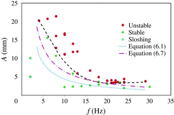
From the experimental results, the values of the critical amplitude were determined as a function of critical frequency. For instance, the value of critical frequency at the onset was obtained by carrying out experiments at a small amplitude and varying the frequency until instability occurs. Then the amplitude was increased gradually with a small frequency change in such a way as to be close to the threshold. We repeated every experiment twice and, as a rule, there was good reproducibility. Figure 16 shows the resulting stability diagram as amplitude versus frequency. The green rhombi indicate experimental parameters near the threshold at which we did not observe instability, while the red circles show experimental points at which interfacial instability was found.
Experimental stability diagram. Symbols define the experimental points and the black dashed curve is a guideline for eyes to illustrate the threshold of instability. The dotted curve shows the threshold of instability defined by the linear theory for immiscible fluids and dashed-dotted line outlines the threshold according to Kelvin–Helmholtz instability in a density stratified fluid.

The black dashed curve is a guideline which delineates the regions of stability and instability. This curve displays a not well-pronounced minimum at
 $f\approx 21~\text{Hz}$
. This finding is in agreement with the observation by Gonzalez-Vinas & Salan (Reference Gonzalez-Vinas and Salan1994) that the amplitude of vibrations to reach the instability onset was first a decreasing function of frequency (prevailing gravity waves) and then an increasing function of
 $f$
(prevailing capillary waves). They reported a deep minimum at
 $f^{\ast }=28~\text{Hz}$
and following strong growth
 $A(f)$
in a capillary regime which was associated with a relatively large surface tension of
 $\text{CO}_{2}$
liquid/vapour system in the near-critical state, at least a few orders of magnitude larger than in the present study. Consequently, the tiny interfacial tension explains a very modest increase in the amplitude at high frequencies in figure 16.
6.2. Comparison with inviscid theory
Lyubimov & Cherepanov (Reference Lyubimov and Cherepanov1987) suggested dispersion relation (1.1) for the case of two immiscible inviscid fluids vibrated horizontally at high frequency,
 ${\it\Omega}\gg 1$
. Since this relation has an analytical form, there exist continuous attempts in the literature to compare the obtained results with this expression regardless of the difference in the basic assumptions. We do the same, although the interfacial tension
 ${\it\sigma}$
is presumably very small. Wunenburger et al. (Reference Wunenburger, Evesque, Chabot, Garrabos, Fauve and Beysens1999) suggested writing (1.1) in a convenient form for comparison of the critical velocity of vibrational forcing
 $$\begin{eqnarray}\displaystyle (A{\it\omega})_{cr}^{2}=\frac{({\it\rho}_{1}+{\it\rho}_{2})^{3}}{{\it\rho}_{1}{\it\rho}_{2}({\it\rho}_{1}-{\it\rho}_{2})}\left[\frac{{\it\sigma}g}{({\it\rho}_{1}-{\it\rho}_{2})}\right]^{1/2} & & \displaystyle\end{eqnarray}$$
when a wave with the critical wavelength
 ${\it\lambda}_{cr}$
develops at the interface between fluids:
 $$\begin{eqnarray}{\it\lambda}_{cr}=2{\rm\pi}\left[\frac{{\it\sigma}}{({\it\rho}_{1}-{\it\rho}_{2})g}\right]^{1/2}.\end{eqnarray}$$
With the purpose of determining the critical wavelength, the experiment at the threshold of instability with
 $f=22~\text{Hz}$
was repeated at least five times, and it was determined that
 ${\it\lambda}_{cr}\approx 0.55\pm 0.05~\text{mm}$
(can be seen in figure 6 at
 $t=8~\text{s}$
). This value is well supported by the calculations of the averaged equations, see figure 7(g). Combining (6.1) and (6.2) the critical velocity can be expressed via the measurable wavelength and the values of densities listed in table 1
 $$\begin{eqnarray}\displaystyle (A{\it\omega})_{cr}^{invis}=\sqrt{\frac{({\it\rho}_{1}+{\it\rho}_{2})^{3}}{{\it\rho}_{1}{\it\rho}_{2}({\it\rho}_{1}-{\it\rho}_{2})}\frac{{\it\lambda}_{cr}g}{2{\rm\pi}}}=0.288. & & \displaystyle\end{eqnarray}$$
The blue dotted curve in figure 16 corresponds to (6.3), in particular,
 $(Af)_{cr}=0.046$
. The curve lies well below the experimentally determined threshold of instability. Furthermore, the curvature of the experimental trend curve (dashed black) cannot be described by the constant product
 $(a{\it\omega})$
as predicted by (6.1)–(6.3). The experiments by Talib et al. (Reference Talib, Jalikop and Juel2007) in immiscible fluids found that the inviscid model (i.e. (6.1)) underestimated the threshold for fluids of a small viscosity contrast, but overestimated the threshold for fluids of high viscosity contrast. Our experimental results shown in figure 16 support their conclusion that for liquids with a small viscosity contrast (
 ${\it\nu}=2.3$
), the inviscid theory underestimates the threshold. The authors of other experiments with immiscible fluids of large viscosity contrast
 ${\it\nu}\approx 100$
(Ivanova et al.
Reference Ivanova, Kozlov and Evesque2001) reported a good agreement with (6.1) when
 ${\it\Omega}>200$
. Our results in figure 16 suggest a reasonable qualitative agreement at the high frequencies when
 ${\it\Omega}>350$
(
 $f>15~\text{Hz}$
).
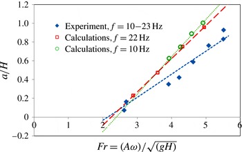
6.3. Dependence on the Froude number
After the
 ${\it\Pi}$
theorem, the threshold of the frozen wave instability depends on five dimensionless parameters, composed of the surface tension
 ${\it\sigma}$
, Earth’s gravity
 $g$
, viscosity
 ${\it\nu}_{i},$
density
 ${\it\rho}_{i}$
, (
 $i=1,2$
) and the thickness of each layer
 $H$
. The critical value of the vibrational Froude number,
 $Fr_{cr},$
can be presented as a function of the other four parameters
 $$\begin{eqnarray}Fr=\frac{A{\it\omega}}{\sqrt{gH}},\quad Fr_{cr}=F\left({\it\nu},{\it\rho},\frac{{\it\sigma}}{{\it\rho}_{i}(g{\it\nu}_{i})^{2/3}},\frac{A}{H}\right).\end{eqnarray}$$
All the experiments were performed using the same liquid system, correspondingly, viscosity
 ${\it\nu}$
and density
 ${\it\rho}$
contrasts are constant and the instability will be characterized by the Froude number,
 $Fr$
, and ratio
 $A/H.$
Maximal height of the wave against of the vibrational Froude number,
 $Fr=A{\it\omega}/\sqrt{gH}$
. The rhombi show experimental points when forcing frequency changes from 10 to 23 Hz. Numerical results correspond to frequencies
 $f=10~\text{Hz}$
(circles) and
 $f=22~\text{Hz}$
(squares) while amplitude
 $A$
is varied. Lines indicate the linear fit of the points.

Hereafter, we will compare the measured threshold with that of the classical Kelvin–Helmholtz instability for a linearly changing distribution of density in the absence of surface tension. This is given by the Richardson number,
 $Ri=gH/U_{ch}^{2}=gH/(A{\it\omega})^{2},$
here
 $U_{ch}=A{\it\omega}$
. Typically the interface is unstable for
 $Ri<0.25$
(Chandrasekhar Reference Chandrasekhar1981). Considering the relation between the Richardson and Froude numbers,
 $Ri=1/Fr^{2}$
, the instability should emerge when
 $$\begin{eqnarray}Ri=1/Fr^{2}<0.25\quad \text{or}\quad Fr_{cr,theory}>2.\end{eqnarray}$$
Figure 17 shows the dependence of the maximal wave height
 $a$
(defined in figure 15) normalized by the layer thickness
 $H$
as function of the vibrational Froude number. The symbols indicate experimental (filled rhombi) and numerical (open symbols) points while the straight lines show the linear fit. The experimental points correspond to the range of forcing frequencies from 10 to 23 Hz. The most striking result is that by varying both the frequency and amplitude of forcing, we found that the critical value of the Froude number for the onset of the frozen wave instability linearly decreased toward a constant threshold,
 $$\begin{eqnarray}Fr_{cr,exp}=(A{\it\omega})_{cr}^{Fr}/\sqrt{gH}=2.14\pm 0.05.\end{eqnarray}$$
This value is in an excellent agreement with the predictions of the classical Kelvin–Helmholtz instability, expressed by (6.5).
The numerical results show that the slopes of the linear fits differ depending on whether the graph was built at a constant amplitude or a constant frequency, rather than on their product
 $(A{\it\omega})$
. The computer simulations for two distinctive frequencies
 $f=10~\text{Hz}$
(circles) and
 $f=22~\text{Hz}$
(squares) display different slopes between them as well as with the experimental trend line. However, the critical values
 $Fr_{cr}(f=22~\text{Hz})=2.24$
and
 $Fr_{cr}(f=10~\text{Hz})=2.38$
are only approximately 5 % and 10 % larger than the experimental one. The experimental line is closer to the numerical one at a higher frequency. Moreover, the experimental rhombus corresponding to
 $f=22~\text{Hz}$
(
 $Fr=2.68$
) lies on the numerical trend line for the same frequency, illustrating an excellent agreement between the experimental and numerical results. Note that all approaches provide
 $Fr_{cr}>2$
.
Similar to inviscid linear theory for immiscible fluids, (6.6) also suggests that at the threshold, the critical velocity
 $U_{cr}=(A{\it\omega})_{cr}$
is constant. Using a value of
 $Fr_{cr,exp}=2.14$
, the critical velocity can be determined as
 $$\begin{eqnarray}\displaystyle (A{\it\omega})_{cr}^{Fr}=Fr_{cr}\sqrt{gH}=0.41,\quad \text{or}\quad (Af)_{cr}=0.065. & & \displaystyle\end{eqnarray}$$
This dependence is presented in the stability diagram in figure 16 by the dashed-dotted curve and it provides a moderately better agreement with the experimental critical curve than (6.1).
6.4. Determination of interfacial tension between miscible liquids
It is interesting to note that the vibrational experiments allow us to determine the interfacial tension
 ${\it\sigma}$
between miscible liquids from the experimental data at the threshold time
 $t_{0}$
. Using the relation (6.2), and the measured critical wavelength, an interfacial tension can be found from the formula
 $$\begin{eqnarray}{\it\sigma}=\left(\frac{{\it\lambda}_{cr}}{2{\rm\pi}}\right)^{2}({\it\rho}_{1}-{\it\rho}_{2})g=(5.84\pm 1.05)\times 10^{-6}~\text{N}~\text{m}^{-1}.\end{eqnarray}$$
The recent review by Vorobev (Reference Vorobev2014) made a point that the measured dynamic interfacial tension between miscible liquids changes in the range of
 $10^{-4}$
–
 $10^{-7}~\text{N}~\text{m}^{-1}$
depending on the liquids and techniques. Our value of the interfacial tension
 ${\it\sigma}\sim 6\times 10^{-6}~\text{N}~\text{m}^{-1}$
falls in this range. It was also mentioned in the same review that the accuracy of several techniques suffer from transient behaviour of the interfacial tension. In this sense, vibrational experiments are advantageous as they are very fast, the delay time for instability emergence is very small,
 $t_{0}\sim 2{-}5~\text{s}$
.
7. Conclusions
In the present work we have performed an extensive experimental and computational study of interfacial instability between two miscible liquids of similar (but non-identical) viscosities and densities subjected to horizontal vibrations. This is one of the first vibrational experimental studies with ordinary miscible liquids separated by a sharp interface. The focus was to observe the development and decay of frozen waves, and to examine their nonlinear dynamics. Instability in miscible systems is noticeably different from immiscible ones because of its transient nature; the difference in density across the interface and the effective interfacial tension decrease over time. One of the features that highlights the difference between immiscible and miscible fluids is the shape of frozen waves. We have provided an explanation that vanishing interfacial tension is responsible for triangular-shaped waves while for immiscible fluids this shape is known to be sinusoidal.
On the numerical side we have obtained solutions to the full Navier–Stokes equations and equations in the averaging approach with a separation of time scales. The averaged equations allow direct computation of the mean (streaming-like) flow. The numerical model for the mean flow is limited to a 2-D study because the simulations of 3-D full equations have shown that the problem is essentially 2-D. Consideration of mean flows suggest a physical explanation for the emergence of waves along the contact line. Three distinctive regimes of the mean flow, repeating over time, allow not only the mechanism of wave formation to be revealed, but also to shed light on the modulation of the interfacial waves predicted theoretically by Varas & Vega (Reference Varas and Vega2007). By tracing the trajectories of particles, we have managed to extract from the experiments detailed information on the mean flow pattern; this strongly supports the physical explanations made on the basis of the numerical results.
Due to the viscous dissipation and limited length of the experimental cell, at long times, the attenuation of interfacial instability starts from the regions near the endwalls and extends toward the centre from the opposite sides, squeezing the wavy pattern. Although the viscous mean flows are coupled to the dynamics of the interfacial waves, they cannot describe this weakening of instability because the averaged equations do not take into account the existence of Stokes boundary layers. The solutions of full Navier–Stokes equations show remarkable agreement with the experimentally observed decay of waves with time, which begins at the endwalls.
As with immiscible liquids, the interfacial instability in miscible liquids has a threshold. With an increase in the value of the oscillatory velocity, the amplitudes of the perturbations grow continuously, forming a saw-tooth frozen structure. By means of optical observations, we have constructed a vibrational forcing map
 $A(f)$
delineating the regions of stability and instability. The comparison of these results with the theoretical prediction by Lyubimov & Cherepanov (Reference Lyubimov and Cherepanov1987) for immiscible liquids has shown that the inviscid model significantly underestimates the threshold of instability. The agreement is better in the region of high frequencies,
 ${\it\Omega}>350$
.
Comparing our results with the Richardson criteria for Kelvin–Helmholtz instability, we have found a much better agreement. Although our numerical simulation showed that the critical Froude number is frequency–amplitude dependent, its generalized experimental value
 $Fr_{cr}=2.14$
only slightly exceeds the value
 $Fr=1/\sqrt{Ri}=2$
for Kelvin–Helmholtz instability in the absence of surface tension.
Finally, we have taken advantage of the measured and computed wavelength for a high frequency at the threshold, and determined the interfacial tension between ordinary miscible liquids; the obtained value is
 ${\it\sigma}\sim 6\times 10^{-6}~\text{N}~\text{m}^{-1}$
. The advantage of this approach with respect to other techniques is that the measurements are made shortly after the initial contact of the miscible liquids. The time delay for the interfacial instability to emerge is only a few seconds and the transient interfacial tension is not yet diminished.
Acknowledgements
This work is supported by the PRODEX programme of the Belgian Federal Science Policy Office and ESA. We also acknowledge support of 59th ESA Parabolic flight campaign.