1. Introduction
A hydraulic jump is a natural fluid flow phenomenon that occurs during transition from supercritical/rapid to subcritical/tranquil flow. The two flow conditions are identified from the relative magnitude of inertial and gravitational forces, quantified by the Froude number
 $(Fr=U_{\textit{a}v\textit{g}}/\sqrt{gh}$
, where
 $U_{\textit{a}v\textit{g}}$
is the depth-averaged velocity of flow, g is the acceleration due to gravity and h is the depth of flow). The flow is supercritical for Fr > 1 and subcritical when Fr < 1. The phenomenon is irreversible and manifests as an abrupt increase in liquid free surface height. This is accompanied by significant dissipation of mechanical energy (Altalib, Mohammed & Hayawi Reference Altalib, Mohammed and Hayawi2019) and intense mixing, which impacts the overall flow development in open channels. The energy dissipation reduces the effects of high pressure and velocity and minimises scouring and damage over the flow path (Altalib et al. Reference Altalib, Mohammed and Hayawi2019). In natural and practical occurrences, a hydraulic jump can be a desired outcome, an unwelcome side effect or a mere unavoidable consequence. In all cases, it cannot be ignored and several studies are reported on the physics of a hydraulic jump.
A relatively less explored area is a laminar planar jump that occurs due to viscous dissipation in thin film flows. Since it occurs without any downstream forcing, this type of jump is termed a ‘natural hydraulic jump’ (Dasgupta, Tomar & Govindarajan Reference Dasgupta, Tomar and Govindarajan2015; Dhar, Das & Das Reference Dhar, Das and Das2020). The natural jump is increasingly exploited in industrial operations such as polymer processing, casting, film draining, extrusion, surface cooling, cleaning and coating as these operations are often associated with thin film free surface flows (Charpin, Lombe & Myers Reference Charpin, Lombe and Myers2007; Hsu et al. Reference Hsu, Walker, Frank and Fuller2011; Walker et al. Reference Walker, Hsu, Frank and Fuller2012). It is also relevant during the flow of biological materials (Jossic et al. Reference Jossic, Lefevre, De Loubens, Magnin and Corre2009; Tasoglu et al. Reference Tasoglu, Park, Peters, Katz and Szeri2011a ; Tasoglu et al. Reference Tasoglu, Peters, Park, Verguet, Katz and Szeri2011b ; Hu & Kieweg Reference Hu and Kieweg2012) and geophysical flows such as the flow of sewage, slurry, lava (Muchiri et al. Reference Muchiri, Monnier and Sellier2023) and mud (Huang & Garcia Reference Huang and Garcia1998).
In most cases, the liquids are non-Newtonian with a yield stress and exhibit laminar flow due to the high material viscosity (Johnson Reference Johnson1970; Davies Reference Davies1986). Rheological studies indicate that many of the natural liquids exhibit identical behaviours to processed fluids, e.g. a mud suspension containing 10 % clay by volume exhibits a mechanical consistency similar to yoghurt (Liu & Mei Reference Liu and Mei1994). On the other hand, the past survey (Dasgupta et al. Reference Dasgupta, Tomar and Govindarajan2015; Dhar et al. Reference Dhar, Das and Das2020, Reference Dhar, Ray, Das and Das2021a
,Reference Dhar, Ray, Das and Das
b
,Reference Dhar, Das and Dasc) reveals that both numerical and theoretical studies on natural jumps are mainly reported for water. There are a few studies in power-law liquids (Zhao & Khayat Reference Zhao and Khayat2008; Rai, Dandapat & Poria Reference Rai, Dandapat and Poria2008; Samanta et al. Reference Samanta, Ray, Kaushal and Das2022; Samanta et al. Reference Samanta, Kaushal, Das and Ray2023) but a generalised yield stress (viscoplastic) liquid has rarely been considered (Ogihara & Miyazawa Reference Ogihara and Miyazawa1994; Shu & Zhou Reference Shu and Zhou2006; Zhou, Shu & Stansby Reference Zhou, Shu and Stansby2007; Ugarelli & Federico Reference Ugarelli and Di Federico2007; Samanta et al. Reference Samanta, Das, Ray and Kaushal2024a
,Reference Samanta, Kaushal, Das and Ray
b
). Such liquids do not flow below the yield stress,
 $\tau _{o}$
, and exhibit either a constant viscosity (Bingham plastic (BP) model) or a power-law dependence of viscosity on shear rate (Herschel–Bulkley (HB) model) when the yield stress is exceeded. One of the earliest studies in yield stress liquids was reported by Ugarelli and Federico (Reference Ugarelli and Di Federico2007). They proposed an approximate solution to predict the jump strength (ratio of liquid height just before and after the jump) as well as bottom shear stress and critical depth for fully developed flow both upstream and downstream of the jump. Zhou et al. (Reference Zhou, Shu and Stansby2007) reported a theoretical study on a planar hydraulic jump in a BP liquid. The analysis, based on the study of Shu & Zhou (Reference Shu and Zhou2006), considered thin film flow approximation where the vertical acceleration is negligible compared with the horizontal. Both Shu & Zhou (Reference Shu and Zhou2006) and Zhou et al. (Reference Zhou, Shu and Stansby2007) validated their results with the experimental data of Ogihara & Miyazawa (Reference Ogihara and Miyazawa1994) for bentonite–water suspensions that behave as BP liquids. Recently, the present authors have investigated a natural planar jump in a thin film BP liquid through numerical simulations, shallow flow theory (SFT) and experiments (Samanta et al. Reference Samanta, Das, Ray and Kaushal2024a
). They validated their results on a steady-state free surface profile, jump location and jump strength against their experimental data. They also reported a numerical study on a natural planar jump in HB liquids (Samanta et al. Reference Samanta, Kaushal, Das and Ray2024b
).
It may be noted that a hydraulic jump is primarily used as an energy dissipator in free surface flows. Yet, to date, almost no study has discussed energy dissipation during a hydraulic jump in non-Newtonian liquids, either in turbulent or in laminar flows. In fact, energy dissipation during a planar jump in a viscous Newtonian liquid is also rare (Dhar et al. Reference Dhar, Ray, Das and Das2021b ). The majority of the studies (Chow Reference Chow1959; Hager Reference Hager2013; Som, Biswas & Chakraborty Reference Som, Biswas and Chakraborty2018) are for energy dissipation during a jump in water, the focus being the design of flood control devices for decelerating flow through jump formation. These studies have considered large-scale analysis and assumed an inviscid flow. There are some works on energy dissipation in a turbulent inviscid flow of water over stepped weirs and spillways (Chanson Reference Chanson2001; Gonzalez & Chanson Reference Gonzalez and Chanson2007; Wüthrich Reference Wüthrich2014; Altalib et al. Reference Altalib, Mohammed and Hayawi2019; Zhou et al. Reference Zhou, Wu, Ma and Hu2020) and a few researchers (Saghebian Reference Saghebian2019; Laishram et al. Reference Laishram, Devi, Singh and Kumar2022) have discussed the influence of channel type and shape on energy dissipation.
The present study reports a detailed analysis of energy dissipation during a natural planar jump in a complex free surface flow. The relative energy dissipation with respect to the inlet energy is obtained as a function of the jump parameters using classical one-dimensional hydraulics, which incorporates a kinetic energy correction factor while the jump parameters are estimated from momentum and continuity equations using SFT, by incorporating the momentum correction factor. Both momentum and kinetic energy correction factors are functions of flow rheology, derived analytically as functions of the dimensionless shear zone height and rheological index of the fluid. Thus, through incorporation of a suitable rheological model, the analysis can predict energy dissipation, jump parameters (location and strength) as well as free surface profiles in the supercritical (upstream of jump) and subcritical (downstream of jump) zones for a laminar jump in a HB, BP, power-law and viscous and inviscid Newtonian liquids. The predictions, validated against experimental data and simulated results, are further explored to understand the role of operating parameters and flow rheology on jump characteristics and energy dissipation during laminar flow. The analysis can be used in lieu of complex numerical techniques for a fast solution of engineering problems arising in processing of any time-independent, inelastic liquid. Using this analysis, we can predict (i) conditions for inducing a hydraulic jump to effect enhanced mixing, heat and the mass transfer rate during laminar flow, say in the case of a laminar flow reactor; (ii) ways to avoid it for ensuring uniformity of film thickness, say in the case of a thin film coating; and (iii) means to increase energy dissipation, say, for example, by mixing a shear-thinning polymer with a yield stress liquid or confining the flow to the supercritical region. To the best of the authors’ knowledge, no study to date has discussed energy dissipation for a hydraulic jump in a non-Newtonian liquid.
The remainder of the paper is organised as follows. Section 2 discusses the energy analysis, § 3 describes the flow rheology and § 4 presents the formulation of SFT for a generalised yield stress liquid. The validation of theoretical predictions with numerical and experimental results for fluids obeying different rheological models is presented in § 5. Insights into the flow physics as a function of input parameters and rheological properties are discussed in § 6. The salient conclusions of the study are summarised in § 7.
2. Energy dissipation across jump
Specific energy diagram (Es vs h) and (b) schematic representation of free surface profile (A-1–2-C) during a planar hydraulic jump, where A, 1, 2 and C correspond to the channel inlet, position immediate upstream and downstream of the jump and the channel exit, respectively.

The analysis of energy dissipation during a planar hydraulic jump in an inviscid flow is well documented in standard fluid mechanics text books (Chow Reference Chow1959; Hager Reference Hager2013; Som et al. Reference Som, Biswas and Chakraborty2018). In an open channel, the total mechanical energy of a flowing fluid is generally expressed as specific energy, E s , i.e. the total energy per unit weight of the liquid or the total head of the flowing system, where the reference datum is chosen, such that the potential head is measured from the channel floor (Som et al. Reference Som, Biswas and Chakraborty2018).
Thus, the sum of the potential and pressure heads becomes equal to the height of the free surface, h. As a result,
 $E_{s}$
at any stream-wise location is the sum of liquid depth and velocity head, viz.,
 \begin{equation} E_{s}=h+\frac{\alpha U_{\textit{a}v\textit{g}}^{2}}{2g}=h+\alpha \left(\frac{q^{2}}{2g}\right)\frac{1}{h^{2}} \quad (\text{because } U_{\textit{a}v\textit{g}}h=q) ,\end{equation}
where
 $q$
is the discharge rate per unit width and α is the kinetic energy correction factor
 $[=\int _{0}^{h}u^{3}\,\text{d}y/(hU_{\textit{a}v\textit{g}}^{3})]$
.
From (2.1), specific energy is related to the liquid depth and discharge rate and among E
s
, h and q, the variation of any two parameters fixes the third. It is conventional to keep q constant and vary E
s
with h to obtain figure 1(a), commonly termed as the specific energy diagram. The figure shows that the variation of specific energy with depth occurs between two extremes – the curve becomes asymptotic to the E
s
axis for low values of h, i.e.
 $h\rightarrow 0$
, and the curve becomes asymptotic to the diagonal
 $(E_{s}=h)$
when h is high. The two conditions intersect at the critical point,
 $Fr=1$
, (point C in figure 1
a) where E
s
is the minimum (E
s,min
). The corresponding liquid depth is called the critical depth (h
c
). Thus, the critical point separates the supercritical flow domain (curve AC in figure 1
a) from the subcritical domain (curve BC in figure 1
a).
Since the hydraulic jump (figure 1 b) is a discontinuity (Rayleigh Reference Rayleigh1914), it does not follow the theoretical specific energy diagram monotonically. The depth-energy path is traced in figure 1(a) by the red solid curve superimposed on the black dashed curve. In the figure, the inlet and outlet conditions are denoted by points A and C, respectively. Starting from inlet A marked in figure 1(a), the curve follows the specific energy diagram up to point 1, just upstream of the jump. Then it suddenly shifts to point 2, corresponding to the maximum liquid depth. After the jump, the liquid depth gradually decreases and the energy diagram follows path 2-C.
Applying Bernoulli’s equation across the jump, i.e. across points 1 and 2 located just upstream and downstream of the jump (figure 1
b), the loss of head/specific energy,
 $h_{j}$
, can be expressed as
 \begin{equation} h_{j}={\unicode[Arial]{x0394}} E_{s}=h_{1}-h_{2}+\frac{\alpha \left(U_{\textit{a}v\textit{g},1}^{2}-U_{\textit{a}v\textit{g},2}^{2}\right)}{2g}=h_{1}-h_{2}+\alpha \left(\frac{q^{2}}{2g}\right)\left[\frac{1}{h_{1}^{2}}-\frac{1}{h_{2}^{2}}\right]\! .\end{equation}
Since the upstream and downstream profiles are disconnected, the jump location is identified by connecting the two profiles through the momentum balance equation using Rayleigh shock (Rayleigh Reference Rayleigh1914) (elaborated later). This results in a Bélanger type of equation (2.3) that expresses the jump strength, i.e. the ratio of liquid height immediately downstream and upstream of the jump (
 $h_{2}/h_{1}$
), as a unique function of the upstream Froude number,
 ${\textit{Fr}}_{1}={q}/{\sqrt{g{h_{1}}^{3}}}$
, where
 $h_{1}$
and
 $h_{2}$
(figure 1) are termed as the conjugate depth in hydraulic jump analysis, i.e.
 \begin{equation} \frac{h_{2}}{h_{1}}=\frac{\sqrt{1+8\beta {\textit{Fr}}_{1}^{2}}-1}{2} ,\end{equation}
and
 $\beta$
, the momentum correction factor, at any streamwise location x is
 \begin{equation} \beta =\frac{\left(\int _{0}^{h}u^{2}\rm d y\right)}{\left(h{U_{\textit{a}v\textit{g}}}^{2}\right)}. \end{equation}
On substituting (2.3) into (2.2), the fraction of energy dissipated with respect to the upstream head
 $(E_{s,1})$
is obtained as
 \begin{equation} \frac{{\unicode[Arial]{x0394}} E_{s}}{E_{s,1}}=\frac{\alpha \left(\sqrt{1+8\beta {\textit{Fr}}_{1}^{2}}-3\right)^{3}+8\left(\alpha -\beta \right)\left(\sqrt{1+8\beta {\textit{Fr}}_{1}^{2}}-3\right)\left(\sqrt{1+8\beta {\textit{Fr}}_{1}^{2}}-1\right)}{8\beta \left(2+\alpha {\textit{Fr}}_{1}^{2}\right)\left(\sqrt{1+8\beta {\textit{Fr}}_{1}^{2}}-1\right)}. \end{equation}
Since inlet parameters are usually the known quantities, (2.5) is expressed in terms of the inlet head
 $(E_{s,{\textit{in}}})$
as
 \begin{equation} \frac{{\unicode[Arial]{x0394}} E_{s}}{E_{s,{\textit{in}}}}=\frac{h_{1}}{h_{\textit{in}}}\frac{\alpha \left(\sqrt{1+8\beta {\textit{Fr}}_{1}^{2}}-3\right)^{3}+8\left(\alpha -\beta \right)\!\left(\sqrt{1+8\beta {\textit{Fr}}_{1}^{2}}-3\right)\left(\sqrt{1+8\beta {\textit{Fr}}_{1}^{2}}-1\right)}{8\beta \left(2+\alpha {\textit{Fr}}_{\textit{in}}^{2}\right)\left(\sqrt{1+8\beta {\textit{Fr}}_{1}^{2}}-1\right)}. \end{equation}
Another important parameter in the analysis of energy dissipation is jump efficiency, the ratio of downstream to upstream head, which can be expressed as
 \begin{equation} \frac{E_{s,2}}{E_{s,1}}=\frac{\left(1+8\beta {\textit{Fr}}_{1}^{2}\right)^{3/2}+3\sqrt{1+8\beta {\textit{Fr}}_{1}^{2}}+4\left(\alpha -6\beta \right){\textit{Fr}}_{1}^{2}-4}{\left(2+\alpha {\textit{Fr}}_{1}^{2}\right)\left(2+8\beta {\textit{Fr}}_{1}^{2}-2\sqrt{1+8\beta {\textit{Fr}}_{1}^{2}}\right)} .\end{equation}
In this study, energy dissipation is discussed only in terms of
 ${\unicode[Arial]{x0394}} E_{s}$
to avoid repetition.
It may be noted that the same expressions (2.5)–(2.7) for energy dissipation and jump efficiency are obtained by Dhar et al. (Reference Dhar, Ray, Das and Das2021b
) for Newtonian liquids. However, the expressions of
 $\alpha$
and
 $\beta$
are different for Newtonian and non-Newtonian liquids as they depend on velocity profile. In an inviscid flow,
 $\alpha =\beta =1,$
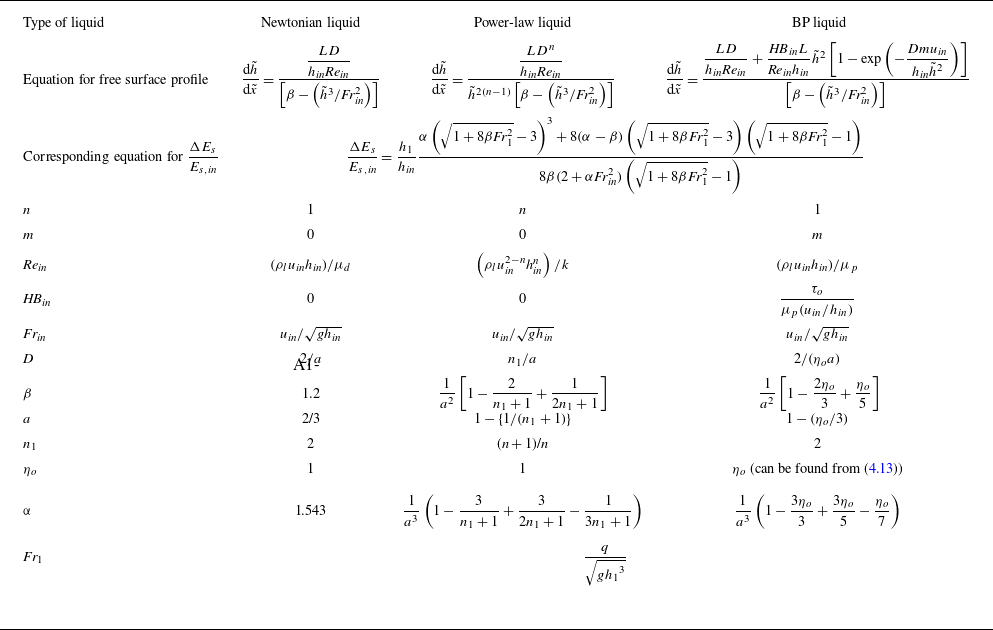
i.e. the flow is uniform while in viscous flow, the non-uniform velocity profile is incorporated through the kinetic energy and momentum correction factors. In the present study they are obtained from SFT for a generalised viscoplastic liquid shown later by (4.14) and (4.15). Using suitable limiting conditions, they can be predicted for BP, power-law and Newtonian liquids.
3. Flow rheology
A generalised viscoplastic liquid is commonly described by the HB model, viz. ((3.1a ) and (3.1b )):
 \begin{align} \underline{\underline{\tau }}& =\left[\frac{\tau _{o}}{\left| \dot{\gamma }\right| }+k\left| \dot{\gamma }\right| ^{n-1}\right]\underline{\underline{\dot{\gamma }}}\quad \mathrm{for}\,\,\left| \tau \right| \gt \tau _{o}, \end{align}
 \begin{align}\dot{\gamma }&=0\quad\mathrm{for}\,\,\left| \tau \right| \leq \tau _{o}. \end{align}
Here the double underline denotes the tensor quantities and
 $\tau$
is the shear stress.
 $\dot{\gamma },k$
and
 $n$
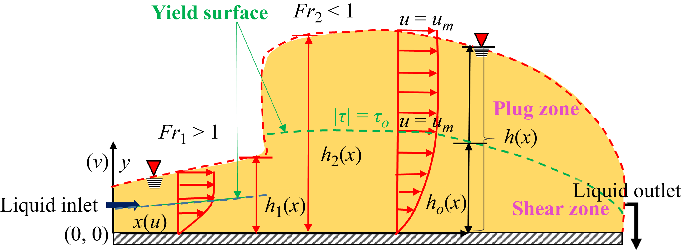
denote the shear rate, flow consistency index and flow behaviour index, respectively. The presence of yield stress divides the flow domain into two regions as shown in figure 2: (i) a shear zone of height
 $h_{o}(x)$
where
 $| \tau | \gt \tau _{o}$
, and (ii) a plug zone of height
 $h_{p}(x)=h(x)-h_{o}(x)$
where
 $| \tau | \leq \tau _{o}.$
In the shear zone, liquid undergoes viscous deformation and the velocity profile u(x) is a function of the flow behaviour index, n, varying from 0 at the channel floor to
 $u_{m}$
(maximum velocity) at the yield surface,
 $(| \tau | =\tau _{o})$
. In the plug zone, the liquid does not encounter any viscous deformation and the velocity
 $u_{p}$
remains constant across the flow although it varies in the flow direction due to a change in film thickness. To maintain velocity continuity at the yield surface, the plug zone velocity,
 $u_{p}$
, is equal to the maximum velocity in the shear zone,
 $u_{m}$
, at any streamwise location, x. The plug zone disappears for
 $\tau _{o}=0$
and the equation reduces to the power-law model where
 $n\lt 1$
signifies pseudoplastic/shear-thinning behaviour and
 $n\gt 1$
denotes dilatant/shear-thickening behaviour. Likewise, the BP model (linear shear stress versus shear rate relationship) is obtained for
 $n=1$
and
 $\tau _{o}\neq 0$
.
Schematic representation of a natural hydraulic jump in a HB fluid. The yield surface
 $(| \tau | =\tau _{o})$
is denoted by the green dashed line. Here u and v are the streamwise (x-directional) and the vertical (y-directional) component of velocity. Subscripts ‘1’ and ‘2’ denote the locations immediate upstream and downstream of the jump. The flow is supercritical (Fr
1
> 1) upstream of the jump and subcritical (Fr
2
< 1) after the jump. The respective heights of the shear zone and the liquid film are h
o
and h. Throughout the flow, the velocity increases from zero at the channel floor to u
m
at the yield surface, and the velocity in the plug region remains constant at u
m
, the maximum velocity of the shear zone.

It may be noted that the ideal viscoplastic model (3.1) offers separate constitutive relations for the plug and shear zone, resulting in a singularity while approaching the yield surface (
 $| \dot{\gamma }| \rightarrow 0$
). This has been addressed in literature (Bercovier & Engelman Reference Bercovier and Engelman1980; O’Donovan & Tanner Reference O’Donovan and Tanner1984; Papanastasiou Reference Papanastasiou1987; Di Federico Reference Di Federico1998; Frey et al. Reference Frey, Link, Naccache and Fonseca2016; Mitsoulis & Tsamopoulos Reference Mitsoulis and Tsamopoulos2017; Mehmood et al. Reference Mehmood, Mahmood, Majeed and Awan2021) and our previous studies (Samanta et al. Reference Samanta, Das, Ray and Kaushal2024a
,Reference Samanta, Kaushal, Das and Ray
b
) by the Papanastasiou regularisation parameter, m, which ensures that the yield stress liquid exhibits an infinitely high viscosity in the limit of low shear rates and transitions to a nonlinear stress–strain relationship for
 $| \tau | \gt \tau _{o}$
, thus rendering the original discontinuous model into a continuous one (3.2a
,
b
):
 \begin{equation} \underline{\underline{\tau }}=\left[\frac{\tau _{o}}{\left| \dot{\gamma }\right| }\left[1-\exp \left(-m\left| \dot{\gamma }\right| \right)\right]+k\left| \dot{\gamma }\right| ^{n-1}\right]\underline{\underline{\dot{\gamma }}}.\,\,\,\,\,\,\,\mathrm{for}\,\,\mathrm{all}\,\,\dot{\gamma }. \end{equation}
This gives the expression of apparent viscosity
 $\mu _{\textit{app}}$
as
 \begin{equation} \mu _{\textit{app}}=\frac{\tau _{o}}{\left| \dot{\gamma }\right| }\left[1-\exp \left(-m\left| \dot{\gamma }\right| \right)\right]+k\left| \dot{\gamma }\right| ^{n-1}\,\,\,\,\,\,\,\,\mathrm{for}\,\,\mathrm{all}\,\,\dot{\gamma }. \end{equation}
Equation (3.2a
) reduces to the HB model (3.1a
) when
 $m\rightarrow \infty$
and predicts the power-law behaviour for
 $m=0.$
Based on literature (Frey et al. Reference Frey, Link, Naccache and Fonseca2016; Mitsoulis & Tsamopoulos Reference Mitsoulis and Tsamopoulos2017; Mehmood et al. Reference Mehmood, Mahmood, Majeed and Awan2021) and our past studies, we adopt m = 1000 s. Nevertheless, our numerical simulations for BP (Samanta et al. Reference Samanta, Das, Ray and Kaushal2024a
) and HB liquids (Samanta et al. Reference Samanta, Kaushal, Das and Ray2024b
) have shown that the free surface profiles are insensitive to m for 0.5 s ≤ m ≤ 1000 s. The details of the simulation are given in § 5.2.
4. Shallow flow theory
4.1. Formulation
We consider a steady-state fully developed flow of an incompressible liquid in a wide horizontal rectangular channel (figure 2). Liquid enters the channel with uniform velocity
 $u_{\textit{in}}$
through a narrow opening of height,
 $h_{\textit{in}}$
(
 $\lt \lt W,L$
, where W and L are the width and length of the channel, respectively) and the height of the film at any streamwise position is
 $h(x)$
.
The assumptions in formulation of the SFT using the rheological model, (3.2a , b ) are as follows.
-
(i) Variation of velocity and film thickness across flow (y direction) is negligible compared with the streamwise (x) direction, i.e.
 $v\lt \lt u$
and
$h=h(x)$
.
-
(ii) Pressure is hydrostatic and momentum dissipation is negligible along x compared with the y direction.
-
(iii) The viscous and gravitational forces dominate over surface tension force. Past studies on Newtonian (Bohr, Putkaradze & Watanabe Reference Bohr, Putkaradze and Watanabe1997; Dhar et al. Reference Dhar, Das and Das2020) and non-Newtonian liquids (Samanta et al. Reference Samanta, Ray, Kaushal and Das2022, Reference Samanta, Kaushal, Das and Ray2023, Reference Samanta, Das, Ray and Kaushal2024a ) have also made the same assumption for a natural jump, which occurs by viscous dissipation.
-
(iv) A self-similar velocity profile upstream and downstream of the jump. This is obtained from our numerical simulations discussed in § 5.2. Past studies on a hydraulic jump in Newtonian (Dhar et al. Reference Dhar, Das and Das2020; Dhar et al. Reference Dhar, Ray, Das and Das2021a ,Reference Dhar, Ray, Das and Das b ,Reference Dhar, Das and Das c ), power-law (Samanta et al. Reference Samanta, Ray, Kaushal and Das2022) and BP liquids (Samanta et al. Reference Samanta, Das, Ray and Kaushal2024a ) also used SFT based on this assumption and obtained satisfactory results.
-
(v) Only shear flow occurs at the inlet, i.e. the plug zone does not form at the channel entry.


Based on the aforementioned assumptions, the mass (4.1) and momentum (4.2) balance equations are expressed as
 \begin{align} \frac{\partial u}{\partial x}+\frac{\partial v}{\partial y}&=0, \end{align}
 \begin{align} u\frac{\partial u}{\partial x}+v\frac{\partial u}{\partial y}&=-g\frac{\text{d}h}{\text{d}x}+\frac{k}{\rho _{l}}\frac{\partial }{\partial y}\left(\left| \frac{\partial u}{\partial y}\right| ^{n-1}\frac{\partial u}{\partial y}\right)-\frac{\tau _{o}}{\rho _{l}}\frac{\partial }{\partial y}\left[\exp \left(-m\left| \frac{\partial u}{\partial y}\right| \right)\right]\! . \end{align}
For a generalised approach, the equations are expressed in non-dimensional form (parameters denoted by tilde) using the scaling parameters, L for horizontal length,
 $h_{\textit{in}}$
for vertical length and
 $u_{\textit{in}}$
for velocity. This gives
 \begin{equation} \frac{\partial \tilde{u}}{\partial \tilde{x}}+\frac{\partial \tilde{v}}{\partial \tilde{y}}=0 \end{equation}
and
 \begin{align} \tilde{u}\frac{\partial \tilde{u}}{\partial \tilde{x}}+\tilde{v}\frac{\partial \tilde{u}}{\partial \tilde{y}}&=-\frac{1}{{\textit{Fr}}_{\textit{in}}^{2}}\frac{\text{d}\tilde{h}}{\text{d}\tilde{x}}+\frac{\left(L/h_{\textit{in}}\right)}{{\textit{Re}}_{\textit{in}}}\frac{\partial }{\partial \tilde{y}}\left(\left| \frac{\partial \tilde{u}}{\partial \tilde{y}}\right| ^{n-1}\frac{\partial \tilde{u}}{\partial \tilde{y}}\right)\nonumber\\&\quad -\frac{\textit{HB}_{\textit{in}}\left(L/h_{\textit{in}}\right)}{{\textit{Re}}_{\textit{in}}}\frac{\partial }{\partial \tilde{y}}\left[\exp \left(-\frac{mu_{\textit{in}}}{h_{\textit{in}}}\left| \frac{\partial \tilde{u}}{\partial \tilde{y}}\right| \right)\right] .\end{align}
Furthermore, the law of conservation of mass implies a constant volumetric flow rate per unit width of the channel (
 $q$
). In dimensionless form, this gives
 \begin{equation} \int \limits_{0}^{\tilde{h}}\tilde{u}\left(\tilde{x},\tilde{y}\right)\text{d}\tilde{y}=1 .\end{equation}
Using (4.5) and the boundary conditions viz., no slip at the channel floor,
 $\tilde{u}(x,0)=0, \tilde{v}(x,0)=0$
, and a zero shear rate at the free surface,
 $\left.\partial \tilde{u}/\partial \tilde{y}\right| _{\tilde{y}=\tilde{h}}=0$
(due to negligible viscosity of air compared with the liquid), (4.3) and (4.4) can be integrated with respect to
 $\tilde{y}$
from 0 to
 $\tilde{h}$
. This gives
 \begin{align} \tilde{U}_{\textit{a}v\textit{g}}\frac{\text{d}}{\text{d}\tilde{x}}\left(\beta \tilde{U}_{\textit{a}v\textit{g}}\right)&=-\frac{1}{{\textit{Fr}}_{\textit{in}}^{2}}\frac{\text{d}\tilde{h}}{\text{d}\tilde{x}}-\frac{\left(L/h_{\textit{in}}\right)}{{\textit{Re}}_{\textit{in}}\tilde{h}}\left[\left| \frac{\partial \tilde{u}}{\partial \tilde{y}}\right| ^{n-1}\frac{\partial \tilde{u}}{\partial \tilde{y}}\right]_{\tilde{y}=0}\nonumber\\&\quad - \frac{\textit{HB}_{\textit{in}}\left(L/h_{\textit{in}}\right)}{{\textit{Re}}_{\textit{in}}\tilde{h}}\left[\exp \left(-\frac{mu_{\textit{in}}}{h_{\textit{in}}}\frac{\partial \tilde{u}}{\partial \tilde{y}}\right)\right]_{\tilde{y}=0}^{\tilde{y}=\tilde{h}} ,\end{align}
since
 $({\partial \tilde{u}}/{\partial \tilde{y}})$
is positive,
 $\left| {\partial \tilde{u}}/{\partial \tilde{y}}\right| ={\partial \tilde{u}}/{\partial \tilde{y}}$
in the present case.
In (4.6),
 $\tilde{U}_{\textit{a}v\textit{g}}$
is the depth average velocity at any
 $\tilde{x}$
, i.e.
 \begin{equation} \tilde{U}_{\textit{a}v\textit{g}}=\left(1/\tilde{h}\right)\int \limits_{0}^{\tilde{h}}\tilde{u}\left(\tilde{x},\tilde{y}\right)\,\text{d}y \end{equation}
and
 $\beta$
is the momentum correction factor, defined as
 \begin{equation} \beta =\frac{\left(\int _{0}^{\tilde{h}}\tilde{u}^{2}\text{d}\tilde{y}\right)}{\left(\tilde{h}{\tilde{U}_{\textit{a}v\textit{g}}}^{2}\right)} .\end{equation}
These (
 $\beta$
and
 $\tilde{U}_{\textit{a}v\textit{g}}$
) can be obtained from the self-similar velocity profile of the liquid. The velocity profile is expressed in terms of similarity parameter (Di Federico Reference Di Federico1998; Ugarelli & Federico Reference Ugarelli and Di Federico2007),
 $\eta =\tilde{y}/\tilde{h}$
, as
 \begin{align} \frac{\tilde{u}\left(\tilde{x},\tilde{y}\right)}{\tilde{u}_{m}\left(\tilde{x}\right)}=f\left(\eta \right)&=\left[1-\left(\frac{\eta _{o}-\eta }{\eta _{o}}\right)^{\frac{n+1}{n}}\right]\quad (0\leq \eta \leq \eta _{o}) \end{align}
 \begin{align} &=1\quad (\eta _{o}\leq \eta \leq 1), \end{align}
where
 $\tilde{u}_{m}=u_{m}/u_{\textit{in}}$
and
 $\eta _{o}$
( = h
o
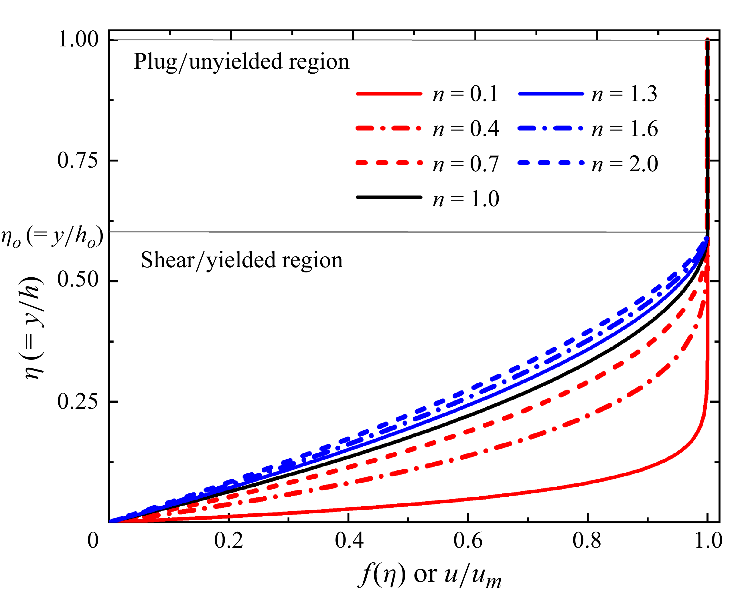
/h) is the fractional thickness of the shear zone compared with the total thickness of the liquid film. Figure 3 shows that the variation of
 $f(\eta )$
with
 $\eta$
at fixed
 $\eta _{o}$
is similar to the distribution reported by Coussot (Reference Coussot1994) for laminar steady flow of a HB liquid. Our numerical simulations have also validated the analytical velocity profile (shown later in figure 8).
Velocity distribution in terms of similarity parameters for a HB fluid with different n at a constant
 $\eta _{o}$
( = 0.6). The position of the yield surface is denoted by a grey line that is extrapolated up to the y/h axis to show the value of the fractional thickness of the shear zone,
 $\eta _{o}=h_{o}/h$
.

Equations (4.5) and (4.7) yield
 $\tilde{U}_{\textit{a}v\textit{g}}\tilde{h}=1$
and by solving (4.5) using (4.9a
) and (4.9b
), we obtain
 \begin{equation} \tilde{U}_{\textit{a}v\textit{g}}=a\tilde{u}_{m} ,\end{equation}
where
 \begin{equation} a=1-\left\{\eta _{o}/\left(n_{1}+1\right)\right\} \end{equation}
and
 \begin{equation} n_{1}=\left(n+1\right)/n .\end{equation}
Thus, the self-similar velocity profile fixes
 $\eta _{o}$
for a particular set of flow and geometric parameters and makes it independent of spatial location. This is also noted from the numerical simulations (shown later in figure 7). So, for a simplistic approach,
 $\eta _{o}$
is obtained from the momentum balance equation for the plug zone (Liu & Mei Reference Liu and Mei1994) that, in scaled form, gives
 \begin{equation} \tilde{u}_{m}\frac{\text{d}\tilde{u}_{m}}{\text{d}\tilde{x}}=-\frac{1}{{\textit{Fr}}_{\textit{in}}^{2}}\frac{\text{d}\tilde{h}}{\text{d}\tilde{x}}-\frac{\textit{HB}_{\textit{in}}\left(L/h_{\textit{in}}\right)}{{\textit{Re}}_{\textit{in}}}\frac{1}{\left(1-\eta _{o}\right)\tilde{h}} .\end{equation}
The numerical simulations (figure 7) also show that the plug zone does not form in the vicinity of the inlet. Thus, the inlet boundary condition is
 $\tilde{h}=\tilde{h}_{o}$
at
 $\tilde{x}=0$
, while at the channel outlet, the flow is taken to be critical, i.e. at
 $\tilde{x}=1,\tilde{h}=\tilde{h}_{c}$
(
 $\tilde{h}_{c}=h_{c}/h_{\textit{in}}$
and
 $h_{c}=(q/\sqrt{g})^{2/3},$
where
 $h_{c}$
is the critical height corresponding to Fr = 1). This is based on past studies of laminar jumps in Newtonian, power-law and BP liquids (Dhar et al. Reference Dhar, Das and Das2020, Dhar et al. Reference Dhar, Ray, Das and Das2021a
,Reference Dhar, Ray, Das and Das
b
,Reference Dhar, Das and Das
c
; Samanta et al. Reference Samanta, Ray, Kaushal and Das2022, Reference Samanta, Das, Ray and Kaushal2024a
). Integrating (4.12), by applying the inlet and outlet boundary conditions and (4.10), we obtain a sixth-order polynomial in terms of
 $\eta _{o}$
(4.13), which upon solving gives only one positive root with
 $\eta _{o}\leq 1$
:
 \begin{equation} \left(1-\eta _{o}\right)\Big(1-\eta _{o}^{2}\Big)\eta _{o}a^{2}-2\left(1-\eta _{o}\right)^{2}+\frac{2\textit{HB}_{\textit{in}}\left(L/h_{\textit{in}}\right)}{{\textit{Re}}_{\textit{in}}}\tilde{h}_{c}\eta _{o}a^{2}=0 .\end{equation}
Applying (4.9a
) and (4.9b
), we have
 $\left.\partial \tilde{u}/\partial \tilde{y}\right| _{\tilde{y}=0}=D/\tilde{h}^{2}$
, where
 $D=n_{1}/(\eta _{o}a)$
and from the velocity profile, the momentum and kinetic energy correction factors are obtained as
 \begin{equation} \beta =\frac{1}{a^{2}}\left[1-\frac{2\eta _{o}}{n_{1}+1}+\frac{\eta _{o}}{2n_{1}+1}\right] \end{equation}
and
 \begin{equation} \alpha =\frac{1}{a^{3}}\left(1-\frac{3\eta _{o}}{n_{1}+1}+\frac{3\eta _{o}}{2n_{1}+1}-\frac{\eta _{o}}{3n_{1}+1}\right) \! .\end{equation}
The analytical derivations of
 $\alpha$
and
 $\beta$
are detailed as follows.
-
(i) Derivation of
$\alpha$
: we have the energy correction factor,
$\alpha ={(\int _{0}^{h}u^{3}\,\text{d}y)}/{(h{U_{\textit{a}v\textit{g}}}^{3})}$
.The analytical velocity profile is
\begin{align*} \frac{\tilde{u}\left(\tilde{x},\tilde{y}\right)}{\tilde{u}_{m}\left(\tilde{x}\right)}&=\frac{u\left(x,y\right)}{u_{m}\left(x\right)}=f\left(\eta \right)=\left[1-\left(\frac{\eta _{o}-\eta }{\eta _{o}}\right)^{\frac{n+1}{n}}\right]\quad &\leq \eta \leq \eta _{o}\notag\\&=1\quad &\eta _{o}\leq \eta \leq 1. \end{align*}
Substituting
$h\,U_{\textit{a}v\textit{g}}=1$
and the analytical velocity profile as mentioned above, we get
\begin{align*} \alpha &=h^{2}\int _{0}^{h}u^{3}dy\notag\\ &=u_{m}^{3}h^{3}\int _{0}^{\eta }\left\{f\left(\eta \right)\right\}^{3}\text{d}\eta \quad(\text{because } u/u_{m}=f\left(\eta \right))\notag\\&=\frac{1}{a^{3}}\left[\int _{0}^{\eta _{0}}\left\{1-\left(\frac{\eta _{o}-\eta }{\eta _{o}}\right)^{{n_{1}}}\right\}^{3}\text{d}\eta +\int _{\eta _{o}}^{1}1.\,\text{d}\eta \right]\!.\notag\\\text{Simplifying},\,\mathrm{we}\,\mathrm{get} & \nonumber \\\alpha &=\frac{1}{a^{3}}\left(1-\frac{3\eta _{o}}{n_{1}+1}+\frac{3\eta _{o}}{2n_{1}+1}-\frac{\eta _{o}}{3n_{1}+1}\right) \!. \end{align*}
-
(ii) Derivation of
$\beta$
: we have the momentum correction factor
\begin{equation*} \beta =\frac{\left(\int _{0}^{h}u^{2}{\rm d}y\right)}{\left(h{U_{\textit{a}v\textit{g}}}^{2}\right)}. \end{equation*}


Simplifying the expression of
 $\beta$
, we get
 \begin{equation*} \beta =\frac{\left(\int _{0}^{h}u^{2}{\rm d}y\right)}{\left(h{U_{\textit{a}v\textit{g}}}^{2}\right)}=h\int _{0}^{h}u^{2}{\rm d}y\quad\left(\text{because } h\,U_{\textit{a}v\textit{g}}=1\right). \end{equation*}
Substituting the velocity profile in the above momentum correction factor equation, we get
 \begin{align*} \beta &=u_{m}^{2}h^{2}\left[\int\limits _{0}^{\eta _{o}}u^{2}\text{d}\eta +\int\limits _{\eta _{o}}^{1}u^{2}\text{d}\eta \right]\quad(\text{because }y/h=\eta ,\quad\text{d}y=h\text{d}\eta )\notag\\&=\frac{1}{a^{2}}\left[\int\limits _{0}^{\eta _{o}}\left\{1-\left(\frac{\eta _{o}-\eta }{\eta _{o}}\right)^{{n_{1}}}\right\}^{2}\text{d}\eta +\int\limits _{\eta _{o}}^{1}1.\,\text{d}\eta \right]\notag\\&\qquad(\text{because } \tilde{U}_{\textit{a}v\textit{g}}=a\tilde{u}_{m};\,\,U_{\textit{a}v\textit{g}}=au_{m};1/h=au_{m})\notag\\& =\frac{1}{a^{2}} \!\left[\int\limits _{0}^{\eta _{o}}\text{d}\eta -2 \!\int\limits _{0}^{\eta _{o}} \!\left(\frac{\eta _{o}-\eta }{\eta _{o}}\right)^{{n_{1}}} \!\text{d}\eta + \!\int\limits _{0}^{\eta _{o}} \!\left(\frac{\eta _{o}-\eta }{\eta _{o}}\right)^{2{n_{1}}} \! \text{d}\eta + \!\int\limits _{\eta _{o}}^{1}1.\,\text{d}\eta \! \right]\!.\notag\\\text{After}\,\text{simplification},& \nonumber \\ & \beta =\frac{1}{a^{2}}\left[1-\frac{2\eta _{o}}{n_{1}+1}+\frac{\eta _{o}}{2n_{1}+1}\right]\!. \end{align*}
Due to the self-similar velocity profile, both
 $\alpha$
and
 $\beta$
remain the same throughout the channel. These are listed in table 1 for different inelastic time-independent non-Newtonian liquids. For Newtonian viscous flow (flow behaviour index n = 1 and an absent plug zone, i.e.
 $\eta _{o}$
= 1), (4.15) gives
 $\alpha =1.543$
, the value reported by Dhar et al. (Reference Dhar, Ray, Das and Das2021b
).
Governing equations and relevant parameters to obtain a steady-state free surface profile and relative energy dissipation for different inelastic time-independent liquids (
 $\mu _{d}$
and
 $\mu _{p}$
are the dynamic viscosity of the Newtonian liquid and the plastic viscosity of the BP liquid, respectively).

4.2. Free surface profile
On introducing the relevant parameters and simplifying (4.6), we obtain
 \begin{equation} \frac{\text{d}\tilde{h}}{\text{d}\tilde{x}}=\frac{{(LD^{n}}/{h_{\textit{in}}{\textit{Re}}_{\textit{in}})}+{(\textit{HB}_{\textit{in}}L}/{{\textit{Re}}_{\textit{in}}h_{\textit{in}})}\tilde{h}^{2n}\left[1-\exp \left(-{Dmu_{\textit{in}}}/{h_{\textit{in}}\tilde{h}^{2}}\right)\right]}{\tilde{h}^{2\left(n-1\right)}\left[\beta -\left(\tilde{h}^{3}/{\textit{Fr}}_{\textit{in}}^{2}\right)\right]} .\end{equation}
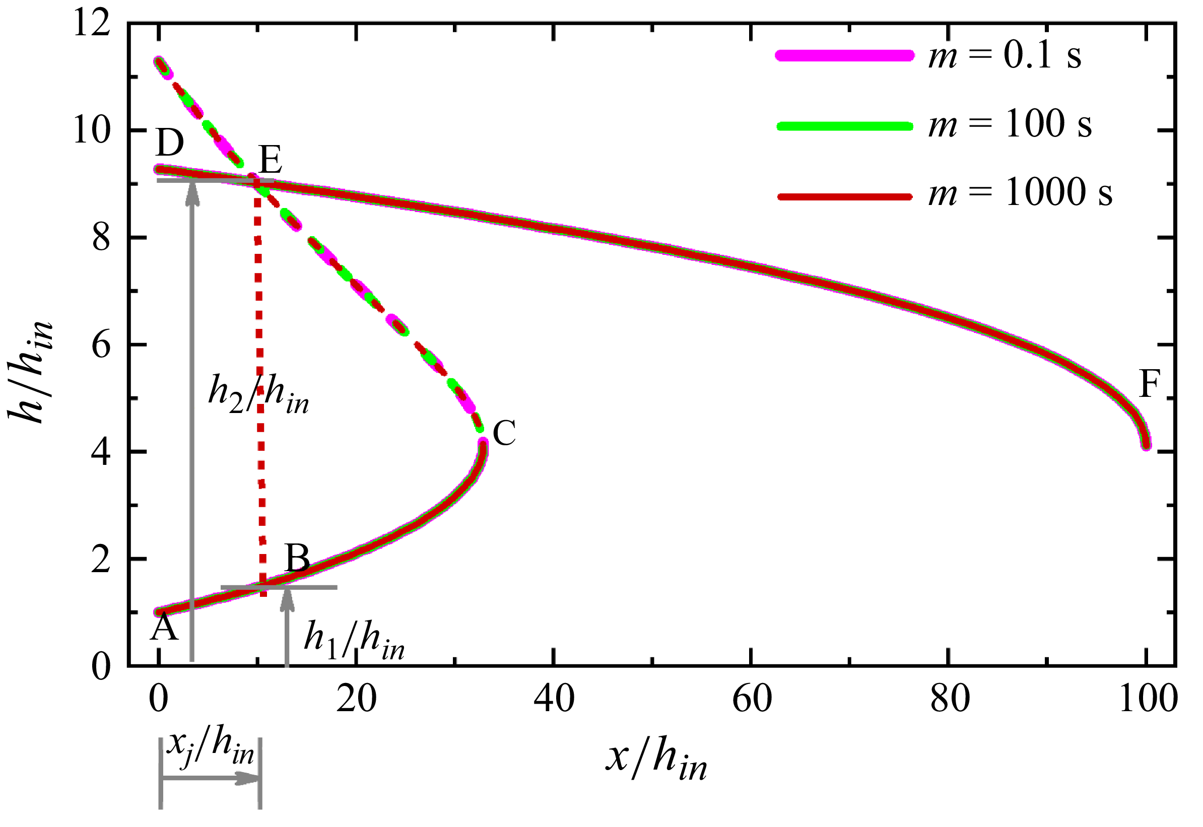
Integrating (4.16) gives the steady-state free surface profile over the entire channel length. However, a close observation shows that (4.16) becomes discontinuous at the critical depth (point C in figure 4), i.e. for
 $\tilde{h}_{c}=(\beta {\textit{Fr}}_{\textit{in}}^{2})^{1/3}$
. We recall that Ugarelli and Federico (Reference Ugarelli and Di Federico2007) also obtained this expression for the critical height in a HB liquid.
Depiction of the solution methodology to evaluate the steady-state free surface profile (curve ABEF), jump location (x/h in -position corresponding to BE) and scaled conjugate depths (h 1 /h in and h 2 /h in ) from SFT. The free surface profiles for three different mvalues (m = 0.1, 100 and 1000 s) are superimposed and so cannot be distinguished.

Taking cue from literature (Dhar et al. Reference Dhar, Das and Das2020; Samanta et al. Reference Samanta, Ray, Kaushal and Das2022; Samanta et al. Reference Samanta, Das, Ray and Kaushal2024a
), this limitation is resolved by integrating (4.16) separately from the inlet to the jump location to obtain the upstream free surface profile (curve AC in figure 4) and from the outlet to the jump location to obtain the downstream profile (curve DF in figure 4). Thus, for the upstream profile, the inlet boundary condition is
 $\tilde{h}=1$
at
 $\tilde{x}=0$
and, for the downstream region, backward integration is performed from slightly before the outlet where the film thickness is
 $h\approx h_{c}$
. The integrations are done numerically using the Runge–Kutta fourth-order method with m = 1000 s, albeit figure 4 showing that the free surface profile obtained from SFT is insensitive to m for 0.1s ≤ m ≤1000 s. The jump location is then identified by connecting the two profiles through the momentum balance equation across the jump using Rayleigh shock (Rayleigh Reference Rayleigh1914) (curve CE in figure 4). This results in a Bélanger type of equation (2.3) as discussed earlier.
On substituting the proper rheological parameters in (4.16), the free surface profiles can be obtained for Newtonian (
 $ \textit{HB}_{\textit{in}}=0$
and n = 1), power-law (
 $ \textit{HB}_{\textit{in}}=0$
) and BP liquids (n = 1). These equations are reported in row 1 of table 1. The same equations were obtained by Dhar et al. (Reference Dhar, Das and Das2020) and Samanta et al. (Reference Samanta, Kaushal, Das and Ray2023, Reference Samanta, Das, Ray and Kaushal2024a
), respectively.
5. Validation
The steady-state free surface profiles and jump parameters (location and strength) are corroborated with our experimental data and numerical simulations. Additionally, the analytical predictions of energy dissipation are validated against our numerical simulations (Samanta et al. Reference Samanta, Kaushal, Das and Ray2024b ).
5.1. Comparison with experimental data
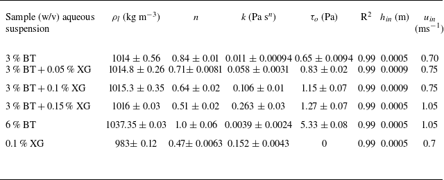
Experiments are performed with a 3 % and 6 % (w/v) aqueous bentonite (BT, Patelnagar Minerals and Industries Pvt. Ltd., West Bengal, India) suspensions and a 0.1 % xanthan gum (XG) solution (Loba Chemicals Pvt. Ltd., India) (Merck Specialities Pvt. Ltd., India). As discussed by Samanta et al. (Reference Samanta, Kaushal, Das and Ray2024b
) (and also shown in table 2), a 3 % BT suspension exhibits a shear-thinning viscoplastic behaviour while a 6 % BT suspension exhibits BP rheology and a 0.1 % XG conforms to power-law model. Furthermore, to obtain viscoplastic liquids with a wide range of
 $\tau _{o}, k$
and
 $n$
, experiments are performed with mixtures of a 3 % BT suspension with different concentrations of aqueous XG solutions (details of the preparation are elaborated in Appendix A). The rheological parameters of the different test liquids are estimated from an Anton Paar modular compact rheometer (MCR-302) using a concentric cylinder geometry having an inner diameter of 5 mm with a 0.2 mm gap. The rheological parameters obtained from the best fit curves (shear stress versus shear rate at room temperature) of the rheological data are listed in table 2. The density, measured at room temperature using a specific gravity bottle, are also included in the table. While all the mixtures have practically the same density, there is a wide variation of rheological parameters, viz., 0.47 ≤ n ≤ 1.0, 0.0039 Pa s
n
≤ k ≤ 0.263 Pa s
n
and
 $0\leq \tau _{o}\leq 5.33\,\mathrm{Pa}$
.
Fluid properties, inlet slit height (
 $h_{\textit{in}}$
) and inlet velocity (
 $u_{\textit{in}}$
) during the experiments.

The experiments are performed in an open rectangular channel of height 2 cm, length 9 cm and width 48.5 cm. The liquid from the tank enters the channel through a narrow slit of height
 $h_{\textit{in}}$
= 0.05 and 0.09 cm. The liquid flow rate per unit channel width, q, is varied from 3.5 × 10⁻⁴ to 6.8 × 10⁻⁴m2 s−1 for the different test liquids and, for each case, the free surface height is measured along the streamwise location by a digital depth micrometre (a resolution limit of 0.1 mm and standard deviation =
 $\pm$
0.02 mm) using the electrical conductance method as adopted by Dhar et al. (Reference Dhar, Das and Das2020, Reference Dhar, Ray, Das and Das2021a
,Reference Dhar, Ray, Das and Das
b
,
Reference Dhar, Das and Dasc
) and Samanta et al. (Reference Samanta, Ray, Kaushal and Das2022, Reference Samanta, Das, Ray and Kaushal2024a
,Reference Samanta, Kaushal, Das and Ray
b
). A similar experimental arrangement was also used by Dhar et al. (Reference Dhar, Das and Das2020), Samanta et al. (Reference Samanta, Ray, Kaushal and Das2022) and Samanta et al. (Reference Samanta, Das, Ray and Kaushal2024a
,Reference Samanta, Kaushal, Das and Ray
b
). The details of the experimental method are described in Appendix A.
Theoretical vis-à-vis experimental steady-state free surface profiles at different q and L/h in for (a) 3 % BT, (b) 3 % BT + 0.05 % XG, (c) 3 % BT + 0.1 % XG, (d) 3 % BT + 0.15 %, (e) 6 % BT and (f) 0.1 % XG. Hollow circles represent experimental data. The upper and lower solid curves correspond to the upstream and downstream profiles obtained from (4.16). The dashed green curve is the profile obtained from the Bélanger equation (2.3) and the red dotted line denotes the jump location.

The measured values of the normalised free surface height (h/h in ) are plotted as a function of the normalised streamwise position from the entry (x/h in ) for the different liquids. Figure 5 depicts some typical results. The free surface profiles obtained from theory are also superimposed on the same figures. The concave solid curve starting from the channel inlet and the upper convex curve extending to the exit denote the respective upstream and downstream profiles obtained from theory (4.16), and the dashed line obtained from (2.3) identifies the jump location by connecting the upstream and downstream profiles through the dotted line. The figure shows good qualitative matching of the free surface profile. The quantitative agreement is also satisfactory both upstream and downstream of the jump, as is confirmed by the maximum deviation ≤ ±10 % except at the jump location. This is expected since the velocity profile changes considerably at the jump and stabilises only when the velocity profile is fully developed. Shallow flow theory cannot capture this due to the assumption of a self-similar profile, which is valid only under fully developed flow conditions. Furthermore, the experimental uncertainty particularly at the jump region is evident from the large error bars in the figures and arises due to significant fluctuation of the free surface. Nonetheless, the theoretically predicted jump location also agrees within ±20 % for power-law, BP and HB liquids.
5.2. Comparison with numerical simulation
5.2.1. Formulation of numerical model
Open channel flow is numerically simulated by considering it equivalent to a partially filled closed rectangular channel. The channel is initially empty (filled with air) and then at time t > 0, liquid flows through a narrow opening close to the channel base. The inlet slit height is sufficiently small compared with the channel height, which ensures a free space above the liquid film within the channel. The incompressible, time-dependent numerical simulation is performed for laminar two-phase air–liquid flow through a rectangular channel using the phase field method in COMSOL Multiphysics® 6.0. The model solves the continuity (5.1), momentum balance (Navier–Stokes) (5.2) and Chan–Hilliard (5.3a and 5.3b ) equations:
 \begin{align} \rho {\boldsymbol{\nabla }}.(\boldsymbol{u})&=0 , \\[-12pt] \nonumber \end{align}
 \begin{align} \rho \frac{\partial \boldsymbol{u}}{\partial t}+\rho (\boldsymbol{u}.{\boldsymbol{\nabla }})\boldsymbol{u}&= {\boldsymbol{\nabla }}.[-pI+\mu ({\boldsymbol{\nabla }}\boldsymbol{u}+{\boldsymbol{\nabla }}\boldsymbol{u}^{T})]+\rho \boldsymbol{g} , \\[-12pt] \nonumber \end{align}
 \begin{align} \frac{\partial \phi }{\partial t}+\boldsymbol{u}.{\boldsymbol{\nabla }}\phi &={\boldsymbol{\nabla }}.\frac{\xi \lambda }{\varepsilon _{pf}^{2}}{\boldsymbol{\nabla }}\psi, \\[-12pt] \nonumber \end{align}
 \begin{align} \psi &=-{\boldsymbol{\nabla }}.\varepsilon _{pf}^{2}{\boldsymbol{\nabla }}\phi +\big(\phi ^{2}-1\big)\phi. \\[9pt] \nonumber \end{align}
Here the bold terms denote vector quantities.
In (5.1)–(5.3),
 $p$
is pressure;
 $I$
is identity matrix;
 $\varphi$
is phase field variable, a smooth function which assumes two different values for two phases, for air:
 $\varphi = -1$
and for HB liquid:
 $\varphi = 1$
and at interface it smoothly varies from
 $-1$
to 1;
 $\xi$
is mobility;
 $\varepsilon_{pf}$
is interface thickness controlling parameter;
 $\lambda$
is mixing energy density; and
 $\psi$
is phase field help variable. The Chan–Hilliard equation is a fourth-order partial differential equation, derived based on the principle of free energy minimisation of the system ensuring mass conservation. Solution of the continuity and momentum balance equations gives pressure, density, viscosity and velocity and the Chan–Hilliard equation provides the spatial phase distribution. The time-dependent governing equations are fully coupled and solved for a sufficient time frame so that steady-state solutions can be obtained for a stationary jump.
Unlike the sharp interface technique, the phase field method works on a diffused interface formulation and yields the sharp interface formulation when
 $\varepsilon _{pf}\rightarrow 0$
. The density ρ and viscosity µ of the air–liquid mixture is expressed in terms of the corresponding phase properties and phase volume fraction V
f
as
 \begin{align} \rho &=\rho _{a}V_{f,a}+\rho _{l}V_{f,l} , \\[-12pt] \nonumber \end{align}
 \begin{align} \mu &=\mu _{a}V_{f,a}+\mu _{\textit{app}}V_{f,l} ,\\[9pt] \nonumber \end{align}
where the the apparent viscosity of the HB liquid (
 $\mu _{\textit{app}}$
) is given by (3.2b
). In (5.4) and (5.5), subscripts ‘a’ and ‘l’ denote air and liquid, respectively.
The phase volume fractions are directly related to
 $\phi$
as
 $V_{f,a}=(1-\phi )/2$
and
 $V_{f,l}=(1+\phi )/2$
, which further signify that at the interface
 $V_{f,a}=V_{f,l}=0.5$
, i.e.
 $\phi =0$
.
COMSOL is based on a finite element method where the problem is solved with the PARDISO solver. The schematic representation of the computational domain (ABCDA) along with the initial and boundary conditions is shown in figure 6. The computational domain (ABCDA) is discretised with a triangular mesh (the minimum element size is
 $4\times 10^{-5}$
cm and the maximum element size is
 $1.34\times 10^{-2}$
cm) under a ‘physics controlled’ meshing option, which inherently incorporates fine grids near the solid boundary to accurately capture the physics of thin film flow. The grid size is chosen based on the results of the grid-independence test that compares different key parameters like pressure, velocity and liquid volume fraction within the liquid film over time for different grid options. The steady-state free surface profiles are also compared for these grids. The details of this exercise are provided in Samanta et al. (Reference Samanta, Kaushal, Das and Ray2024b
).
Schematic representation of the computational domain (rectangular channel ABCDA) with initial and boundary conditions. The yellow portion represents the liquid film and the remaining portion is filled with air. Here H is the height of the channel of length L and h
in
(AE) is the height of the inlet opening. The jump location (x
j
) and upstream (h
1
) and downstream (h
2
) heights are marked in the figure. In the wetted wall condition,
 $\hat{n}$
is the unit normal outward vector from the surface and
 $\theta _{w}$
is the contact angle of liquid with solid in the presence of air. Here p
hyd
is the hydrostatic pressure of the liquid.

5.2.2. Typical results to justify SFT assumptions
The simulated results are shown for two typical cases,
 $n=0.4$
and
 $n=0.7$
, in figures 7(a) and 7(b), respectively. Profiles upstream and downstream of the jump are shown by red and blue curves, respectively. We note that in the upstream section, the profile (red curves) develops right from the entry and on undergoing a jump, it changes considerably depending on the presence of vortices, which results in waviness at the free surface. Far away from the jump, the profiles (blue curves) in the downstream region do not vary and the fractional thickness of the shear zone,
 $\eta _{o}$
(
 $=\tilde{h}_{o}/\tilde{h}$
, where
 $\tilde{h}_{o}=h_{o}/h_{\textit{in}}$
and
 $0\leq \eta _{o}\leq 1$
) becomes practically constant. The yield surface (the locus of
 $h_{o})$
is depicted by the grey horizontal line, where u ≈ 0.99 u
m
. Both figures display a self-similar velocity profile with constant
 $\eta _{o}$
(
 $\approx 0.38$
in figure 7
a and
 $\approx 0.5$
in figure 7
b) in the downstream section where the flow becomes fully developed. This confirms the SFT assumption of a self-similar velocity profile with constant
 $\eta _{o}$
. For the conditions in figure 7, the flow does not become fully developed upstream of the jump as a sufficient developing length is not available before the jump. A close observation also reveals that no plug zone is formed just after the entry, i.e.
 $\eta _{o}| _{x\approx 0}=1$
.
Steady-state velocity profiles from numerical simulations at different axial locations for (a) n = 0.4, HB
in
= 0.3, Fr
in
= 12, Re
in
= 250 and L/ h
in
= 180, where the scaled jump location x
j
/h
in
= 18; (b) n = 0.7, HB
in
= 0.15, Fr
in
= 10, Re
in
= 200 and L/ h
in
= 180, where x
j
/h
in
= 29. The red and blue curves indicate the velocity profile upstream and downstream of the jump. The position of the yield surface for the fully developed downstream velocity profile (blue curves) is denoted by the grey line, its ordinate (y/h) signifying the value of the fractional thickness of the shear zone,
 $\eta _{o}=h_{o}/h$
.

5.2.3. Validation of analytical predictions of SFT
Velocity profile: a comparison of the velocity profiles from SFT and numerical simulations confirms the presence of the yield zone for the viscoplastic test liquids and the absence of the same for the power-law liquid. This is evident from figure 8(a–d) for 0.1 % XG, 0.1 % XG + 3 % BT, 0.05 % XG + 3 % BT and 3 % BT, respectively (rheological properties in table 2). The velocity profiles and location of the yield surface (grey line) obtained from SFT and simulation are identical in the experimentally investigated range of fluid rheology (0.47 ≤ n ≤ 1.0, 0.0039 Pa s
n
≤ k ≤ 0.263 Pa s
n
and
 $0\leq \tau _{o}\leq 5.33\,\mathrm{Pa}$
), flow velocity (q = 3.5 × 10⁻⁴ to 6.8 × 10⁻⁴m2 s−1) and geometric parameters (channel length = 9 cm, inlet height = 0.05 and 0.09 cm). The thickness of the shear zone varies from 15 % to 100 % of the total film thickness (
 $0.15\leq \eta _{o}\leq 1$
) and no plug zone, i.e.
 $\eta _{o}=1$
, is observed only in the case of 0.1 % XG that follows the power-law rheology.
Comparison of the velocity profile from SFT and numerical simulation (for the fully developed downstream section) for (a) 0.1 % XG, (b) 0.1 % XG + 3 % BT, (c) 0.05 % XG + 3 % BT, (d) 3 % BT corresponding to conditions as given in table 2. The location of the yield surface is shown in each plot along with the fractional thickness of the shear zone,
 $\eta _{o}$
. The plug and shear zone are labelled in the figures.

Jump parameters: the theoretical and simulated values of the jump location, jump strength and
 $\eta _{o}$
for different input parameters are presented as parity plots in figure 9(a–c). The figures show a good agreement, with the maximum deviation between theoretical and simulated results being ±20 % for
 $\eta _{o}$
and
 $x_{j}$
and ±25 % for jump strength. Nevertheless, a close observation reveals a consistent under-prediction of
 $\eta _{o}$
and an over-prediction of
 $x_{j}$
and
 $h_{2}/h_{1}$
. This can be attributed to the inherent assumptions in SFT discussed in § 4.1.
Parity plots for (a)
 $\eta _{o}$
, (b)
 $x_{j}$
and (c)
 $h_{2}$
/
 $h_{1}$
, obtained from SFT and simulation at different
 ${\textit{Re}}_{\textit{in}} , {\textit{Fr}}_{\textit{in}} , \textit{HB}_{\textit{in}}$
and
 $L/h_{\textit{in}}$
. In each plot, the solid green line is the parity line [
 $\eta _{o,SFT} = \eta _{o,sim}$
in (a),
 $x_{j,\textit{SFT}} = x_{j,\textit{sim}}$
in (b) and
 $(h_{2}/h_{1})_{\textit{SFT}} = (h_{2}/h_{1})_{\textit{sim}}$
in (c)] and the (±) % deviation ranges are marked by the dotted magenta lines.

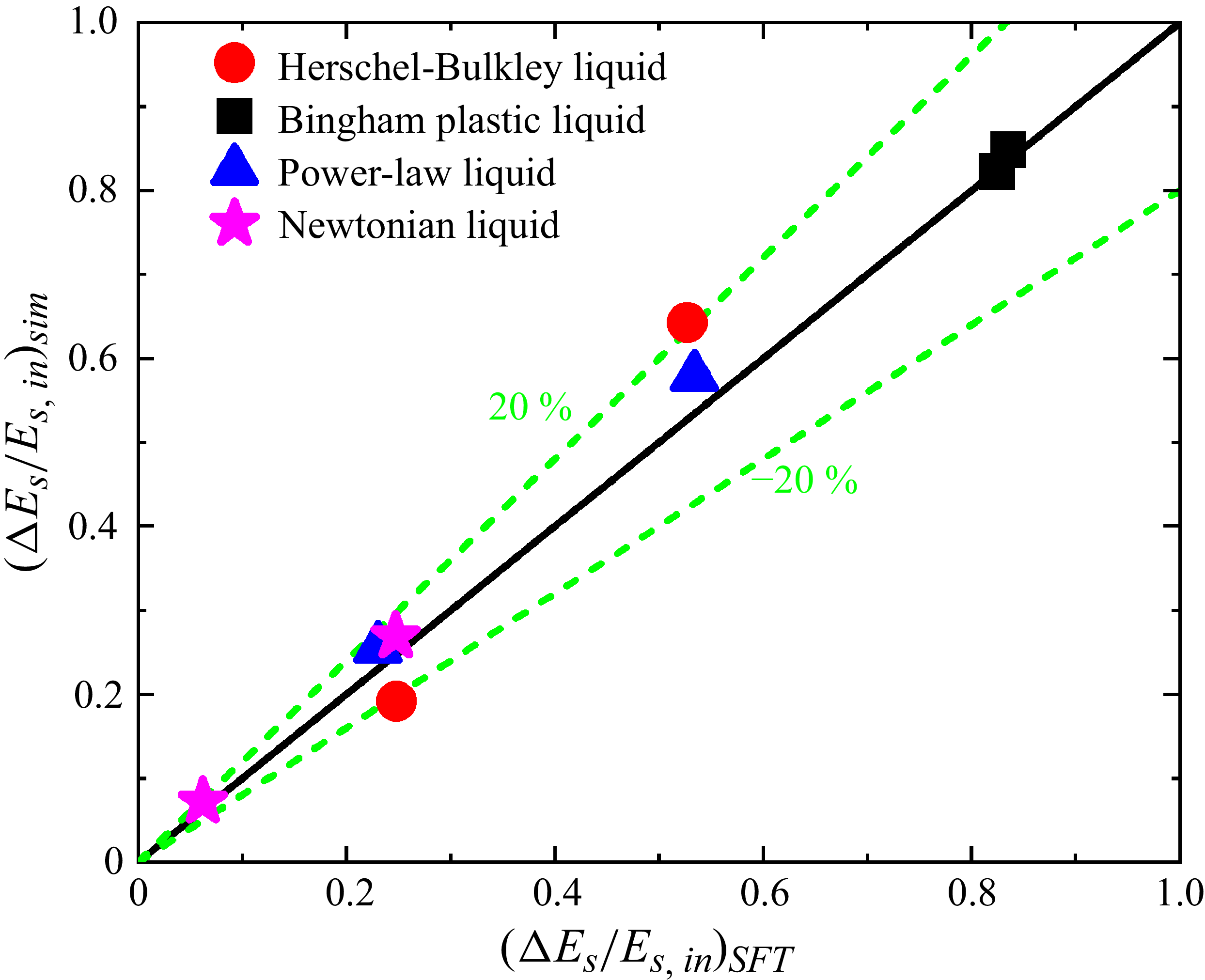
Fractional energy dissipation: figure 10 compares the theoretical and numerical predictions of fractional energy dissipation
 $({\unicode[Arial]{x0394}} E_{s}/E_{s,{\textit{in}}})$
during a natural jump for the test liquids, namely aqueous solutions of 20 % glycerol (
 $\mu _{d}$
= 0.00133 Pa s,
 $\rho _{l}$
= 1040 kg m−3), different concentrations of XG, 6 % BT suspension exhibiting BP behaviour and mixtures of BT and XG that obey HB rheology (rheological data in table 2). Figure 10 shows that the maximum deviation between theory and simulations lie within ±20 %.
Parity plot for the fractional energy dissipation obtained from theory and numerical simulations for four different liquid types: Newtonian, power-law, BP and HB liquids.

6. Physical insights into the jump phenomena
The theoretical analysis, after extensive validations with experimental and numerical predictions, is further explored to obtain physical insights into the jump phenomena. Initially, the influence of flow hydrodynamics on energy dissipation is investigated during a natural jump in a generalised viscoplastic liquid (§ 6.1). Next, the influence of input parameters on the free surface profile before and after the jump, jump location and strength as well as energy dissipation are studied. Since a natural hydraulic jump occurs due to viscous dissipation that predominantly depends on rheological properties of the liquid, we discuss the influence of fluid rheology in § 6.2. Subsequently for a generalised approach, § 6.3 elucidates the influence of input parameters, expressed as non-dimensional numbers. The pertinent non-dimensional numbers are obtained from (4.16) as the HB number,
 $ \textit{HB}_{\textit{in}}= ({\tau _{o}}/{k(u_{\textit{in}}/h_{\textit{in}})^{n}})$
, Froude number,
 ${\textit{Fr}}_{\textit{in}}=u_{\textit{in}}/\sqrt{gh_{\textit{in}}}$
, Reynolds number,
 ${\textit{Re}}_{\textit{in}}=(\rho _{l}u_{\textit{in}}^{2-n}h_{\textit{in}}^{n})/k$
, scaled channel length, L/h
in
, and flow behaviour index, n. Phenomenologically,
 $ \textit{HB}_{\textit{in}} , {\textit{Fr}}_{\textit{in}}$
and
 ${\textit{Re}}_{\textit{in}}$
are the ratios of yield to viscous stress, inertial to gravitational force and inertial to viscous force, respectively.
6.1. Energy dissipation as function of flow hydrodynamics
Equation (2.5) obtains energy dissipation for a HB liquid as a function of the flow behaviour index n, relative thickness of the shear zone
 $\eta _{o}$
and upstream Froude number
 ${\textit{Fr}}_{1}$
, while for a Newtonian liquid, it is a function of
 ${\textit{Fr}}_{1}$
only. The dependence of energy dissipation solely on
 ${\textit{Fr}}_{1}$
for a Newtonian liquid was also reported by Dhar et al. (Reference Dhar, Ray, Das and Das2021b
). Figures 11(a) and 11(b) present the variation of
 ${\unicode[Arial]{x0394}} E_{s}/E_{s,1}$
with
 ${\textit{Fr}}_{1}$
and
 $\eta _{o}$
for different values of n. The results are shown for n ≤ 1 since the test liquids exhibit BP and pseudoplastic yield stress behaviour.
Variation of the fractional energy dissipation with respect to the upstream liquid head (
 ${\unicode[Arial]{x0394}} E_{s}/E_{s,1}$
) as a function of (a) the upstream Froude number Fr
1
at a fixed fractional thickness of the shear zone (
 $\,\eta _{o}=0.5$
), and (b)
 $\,\eta _{o}$
at fixed
 ${\textit{Fr}}_{1}(=5)$
. Both the plots are shown for four different values of n (n = 0.1, 0.4, 0.7 and 1).

The salient observations are as follows.
-
(i) Energy dissipation increases with an increase in all three parameters, although the trend of variation is different for the three cases.
-
(ii) At constant
$\,\eta _{o}$
, the increase is rapid for
${\textit{Fr}}_{1}$
< 5 and becomes gradual for higher values of
${\textit{Fr}}_{1}$
(figure 11
a). A similar trend was also reported by Dhar et al. (Reference Dhar, Ray, Das and Das2021b
) for Newtonian liquids (n =
$\eta _{o}$
= 1). -
(iii) At constant
${\textit{Fr}}_{1}$
,
${\unicode[Arial]{x0394}} E_{s}/E_{s,1}$
exhibits an almost linear increase with
$\eta _{o}$
(figure 11
b) for all values of n. This implies that, for same
${\textit{Fr}}_{1}$
, energy dissipation is higher for liquids with a higher fraction of shear zone, an expected outcome as the shear zone contributes to viscous dissipation. Thus, for constant
${\textit{Fr}}_{1}$
,
${\unicode[Arial]{x0394}} E_{s}/E_{s,1}$
is higher for a power-law liquid compared with a yield stress shear-thinning liquid with the same n. Likewise, for the same
$\eta _{o}$
(same
$\tau _{o}$
),
${\unicode[Arial]{x0394}} E_{s}/E_{s,1}$
is higher for a BP liquid compared with a shear-thinning viscoplastic liquid and a Newtonian liquid exhibits maximum energy dissipation at a particular
${\textit{Fr}}_{1}$
. -
(iv) While
${\unicode[Arial]{x0394}} E_{s}/E_{s,1}$
exhibits a weak dependence on n when
${\textit{Fr}}_{1}$
is varied at constant
$\eta _{o}$
, it is more significantly influenced by n when
$\eta _{o}$
is varied at constant
${\textit{Fr}}_{1}$
. The only exception is at
$\eta _{o}$
< 0.1. The increase in energy dissipation with n at constant
${\textit{Fr}}_{1}$
and
$\eta _{o}$
arises due to an enhanced shearing effect, i.e. viscous dissipation in the shear zone.


Contour plot of
 ${\unicode[Arial]{x0394}} E_{s}/E_{s,1}$
in
 ${\textit{Fr}}_{1}$
vs
 $\eta _{o}$
plane for n = (a) 0.1, (b) 0.4, (c) 0.7 and (d) 1. The magnitude of
 ${\unicode[Arial]{x0394}} E_{s}/E_{s,1}$
is shown by different colours specified in the colour bar beside each figure. Some of the isocontour lines of
 ${\unicode[Arial]{x0394}} E_{s}/E_{s,1}$
are also shown by the grey solid lines.

For a better understanding of the coupled effect of
 ${\textit{Fr}}_{1}$
and
 $\eta _{o}$
on
 ${\unicode[Arial]{x0394}} E_{s}/E_{s,1}$
, the results are presented as contour plots of
 ${\unicode[Arial]{x0394}} E_{s}/E_{s,1}$
in
 ${\textit{Fr}}_{1}$
versus
 $\eta _{o}$
plane for n = 0.1, 0.4, 0.7 and 1 in figure 12(a–d), respectively. For all n, the isocontour of
 ${\unicode[Arial]{x0394}} E_{s}/E_{s,1}$
is nearly vertical for
 ${\textit{Fr}}_{1}$
< 3, signifying a negligible effect of
 $\eta _{o}$
on
 ${\unicode[Arial]{x0394}} E_{s}/E_{s,1}$
in this range of
 ${\textit{Fr}}_{1}$
irrespective of fluid behaviour. However, for
 ${\textit{Fr}}_{1}$
> 3, the isocontour is almost linear with a negative slope, which infers that
 ${\textit{Fr}}_{1}$
and
 $\eta _{o}$
exert an opposite effect on
 ${\unicode[Arial]{x0394}} E_{s}/E_{s,1}$
and that the same amount of energy dissipation is possible with a lower
 $\eta _{o}$
and higher
 ${\textit{Fr}}_{1}$
or vice versa. This happens as a higher
 ${\textit{Fr}}_{1}$
and a lower
 $\eta _{o}$
enhances the dissipation as discussed earlier. Interestingly, the isocontours incline more with an increase in n for
 ${\textit{Fr}}_{1}$
> 3 while for
 ${\textit{Fr}}_{1}$
< 3, the isocontours remain almost unchanged with variation of n. Thus, figures 11 and 12 emphasise that the influence of n,
 $\eta _{o}$
and
 ${\textit{Fr}}_{1}$
is decided by the range of
 ${\textit{Fr}}_{1}$
. For
 ${\textit{Fr}}_{1}$
< 3, the effects of
 ${\textit{Fr}}_{1}$
is more pronounced compared with that of n and
 $\eta _{o}$
while, for
 ${\textit{Fr}}_{1}\gt 5,$
n and
 $\eta _{o}$
influences
 ${\unicode[Arial]{x0394}} E_{s}/E_{s,1}$
more significantly and, for
 $3\lt {\textit{Fr}}_{1}\lt 5,$
, the influence of all three parameters is comparable.
Specific energy diagram for different (a) n at k = 0.04 Pa s
n
,
 $\,\tau _{o}$
= 0.05 Pa, L = 4 cm, h
in
= 0.025 cm, u
in
= 0.45 ms−1; (b) k at n = 0.4,
 $\,\tau _{o}$
= 0.05 Pa, L = 4 cm, h
in
= 0.025 cm, u
in
= 0.40 ms−1; (c)
 $\,\tau _{o}$
at n = 0.4 and k = 0.04 Pa.s
n
, L = 4 cm, h
in
= 0.025 cm, u
in
= 0.40 ms−1. The path followed by the fluid in each case is O–A–B–C, where O represents the inlet, A is immediately upstream of the jump, B is immediately downstream of the jump and C is the exit point, assumed to be at a critical state.

6.2. Effect of rheological parameters
To visualise the effect of rheological parameters (
 $n,k\text{ and }\tau _{o}$
), each of the parameters is varied keeping the other two constant for fixed dimensions of channel geometry and liquid discharge rate.
Figure 13 presents typical specific energy plots and figure 14 shows the corresponding steady- state free surface and the yield surface (where
 $| \tau \,| =\tau _{o}$
) profiles for variation with (i) n at constant
 $\,\tau _{o}$
and k (figure 14
a), (ii) k at constant n and
 $\,\tau _{o}$
(figure 14
b), and (iii)
 $\,\tau _{o}$
at constant n and k (figure 14
c). In the energy plots, the free surface follows path OA in the upstream section (O is the channel inlet and A is immediately upstream of the jump). After the jump, the subcritical flow follows path BC till channel outlet C, which is the critical point with the minimum specific energy. At the jump, the free surface abruptly moves from A to B (shown by the dotted line AB) instead of monotonically following path AC. Points O, A, B and C are also marked in the corresponding free surface profiles in figure 14 for ease of understanding. We note that in the case of a submerged jump that occurs almost at the inlet, i.e.
 $\,x_{j}\approx 0$
, points O and A coincide.
Variation of the steady-state free surface (x vs h) and yield surface (x vs h
o
) profiles for different (a) n at k = 0.04 Pa s
n
,
 $\,\tau _{o}$
= 0.05 Pa, L = 4 cm, h
in
= 0.025 cm, u
in
= 0.45 ms−1; (b) k at n = 0.4,
 $\,\tau _{o}$
= 0.05 Pa, L = 4 cm, h
in
= 0.025 cm, u
in
= 0.40 ms−1; (c)
 $\,\tau _{o}$
at n = 0.4 and k = 0.04 Pa s
n
, L = 4 cm, h
in
= 0.025 cm, u
in
= 0.40 ms−1. Points O, A. B and C represent the inlet, upstream of the jump, downstream of the jump and exit, respectively.

A close observation of figures 13, 14 and 15 reveals the following intriguing features.
Variation of
 $\eta _{o}$
as a function of (a) n at k = 0.04 Pa s
n
,
 $\,\tau _{o}$
= 0.05 Pa, L = 4 cm, h
in
= 0.025 cm, u
in
= 0.45 ms−1; (b) k at
 $\,\tau _{o}$
= 0.05 Pa, L = 4 cm, h
in
= 0.025 cm, u
in
= 0.40 ms−1 for n = 0.4 and 1.0; (c)
 $\,\tau _{o}$
at (n = 0.4 and k = 0.04 Pa s
n
) and (n = 1 and k = 0.0008 Pa s
n
) for L = 4 cm, h
in
= 0.025 cm, u
in
= 0.40 ms−1.

-
(i) Energy dissipation increases with an increase in all three rheological parameters (figure 13), an expected outcome as an increase in any one of the rheological parameters whilst keeping the other two constant increases
$\mu _{\textit{app}}$
(3.1b). Likewise, a jump of higher strength and lower x
j
occurs with increase in
$n,k\text{ and }\tau _{o}$
(figure 14). This arises as a decrease in the average velocity (U
avg
) across the flow due to increased viscous dissipation increases the thickness of the liquid film in order to maintain mass continuity
$(U_{\textit{a}v\textit{g}}h=q)$
. As a result, the jump shifts towards the inlet and due to the lower
$x_{j}$
, h
1
decreases while h
2
increases, resulting in a jump of higher strength, h
2
/h
1
. -
(ii) The energy plots vary significantly with n and
$\,\tau _{o}$
(figure 13) while they are relatively less sensitive to the variation of k. This arises as increasing n increases the fraction of shear zone within the liquid film (
$\eta _{o}$
), while an increase in
$\,\tau _{o}$
increases the plug zone fraction (
$1-\eta _{o}$
). This enhances the uniformity of the velocity profile, approaching the inviscid flow case. Consequently, the energy correction factor,
$\alpha$
, increases with an increase in n and a decrease in
$\tau _{o}.$
On the other hand, the curves for different k superimpose on each other as the velocity profile is independent of k and so
$\alpha$
remains constant. The variation of
$\eta _{o}$
with n, k and
$\,\tau _{o}$
is also evident from figure 15 and discussed later. -
(iii) The critical depth (corresponding to point C) monotonically increases with n. A similar observation was reported by Ugarelli and Federico (Reference Ugarelli and Di Federico2007) for a planar jump in HB liquids. However, the critical depth does not depend on k and monotonically decreases with
$\,\tau _{o}$
, as shown by the magnified plots in figure 13. -
(iv) Interestingly, although the influence of the three rheological parameters appears to be similar, the mechanism of influence is different in the three cases. For a particular x upstream or downstream of the jump, the thicknesses of both the shear zone (h o ) and plug zone (
$h_{p}$
) increase with an increase in
$n\,\,\mathrm{and}\,\,k,\,$
whereas h
o
decreases and
$h_{p}$
increases with an increase in
$\tau _{o}$
. This arises as an increase in n and k increases viscous dissipation, which in turn increases the thickness and intensity of shearing within the shear zone, thus increasing h. However, from figure 14 we note that the thickness of the two zones increases in the same proportion with an increase in k and so
$\eta _{o}$
is independent of k irrespective of n (figure 15). On the other hand, an increase in n increases
$\eta _{o}$
as the shear zone grows more rapidly compared with the plug zone. This is clear from figure 15(a–c). An increase in
$\tau _{o}$
moves the yield surface
$| \tau \,| =\tau _{o}$
closer to the channel floor. This results in a thinner shear zone and a thicker plug zone, thus decreasing
$\eta _{o}$
. A similar variation of the fractional plug zone thickness with yield stress was reported by Wang et al. (Reference Wang, Guo, Ding, Liu, Qin, Wang and Wang2023) for a circular jump. The increase of the shear zone thickness with an increase of n and k and the plug zone thickness with an increase in
$\tau _{o}$
was also noted by Wang et al. (Reference Wang, Guo, Ding, Liu, Qin, Wang and Wang2023) during pipe flow. However, since in that case the flow was under confinement, the plug zone thickness decreased with n and k unlike the present case of free surface flow, where the reverse happens. It may be noted that the influence of k and
$\tau _{o}$
follows the same trend until a submerged jump is formed, subsequent to which the jump location remains unchanged while the jump strength increases. -
(v) Due to the self-similar velocity profile, the qualitative evolution of the yield surface (variation of h o ) and free surface (variation of h) are similar in figure 14. Both h and h o gradually increase from the inlet to x j and then recede towards the exit in the downstream region. In the absence of yield stress, h = h o , hence, the h vs x and h o vs x profiles coincide for
$\,\tau _{o}$
= 0 (figure 14
c).


An additional effort is made to visualise the spatial distribution of specific energy E
s
within the channel when the rheological parameters are varied. This is presented in the form of contour plots of E
s
for different values of n, k and
 $\tau _{o}$
in figure 16(a–c), respectively. In the figures the upstream and downstream zones are demarcated by plotting the corresponding jump location curves (dashed curve). Interestingly, for all cases, the isocontours in the upstream and downstream sections exhibit opposite trends. Their slope is negative in the supercritical (upstream) region and positive in the subcritical (downstream) zone. This signifies that the same value of E
s
can be obtained in the two regions for different combinations of n, k and
 $\tau _{o}$
. In the upstream section, fluids with lower n, k or
 $\tau _{o}$
will experience a given E
s
closer to the exit (higher x) and the opposite situation occurs in the downstream section. Figure 16 also shows that irrespective of the prevailing condition, E
s
always decreases from the inlet to outlet of the channel, confirming irreversible energy loss during flow. Interestingly, the energy loss is always higher in the upstream compared with the downstream section.
Contour plot of the specific energy (E
s
) throughout the channel for different (a) n at k = 0.04 Pa s
n
,
 $\tau _{o}$
= 0.05 Pa, L = 4 cm, h
in
= 0.025 cm, u
in
= 0.45 ms−1; (b) k at n = 0.4,
 $\,\tau _{o}$
= 0.05 Pa, L = 4 cm, h
in
= 0.025 cm, u
in
= 0.40 ms−1; (c)
 $\,\tau _{o}$
at n = 0.4 and k = 0.04 Pa s
n
, L = 4 cm, h
in
= 0.025 cm, u
in
= 0.40 ms−1. Different levels of specific energy are indicated in the colour bar beside each plot. The solid grey lines denote the isocontours of E
s
with the corresponding values. The dashed black curve in panels (a), (b) and (c) represent the jump location
 $x_{j}$
vs n, k, and
 $\,\tau _{o}$
, respectively. The supercritical (upstream) and subcritical (downstream) regions are on the left- and right-hand side of the line in each figure.

6.3. Effect of non-dimensional numbers
The influence of the different non-dimensional numbers is depicted in figures 17 and 18. Figure 17(a–d) shows the influence of
 ${\textit{Re}}_{\textit{in}}$
and
 $L/h_{\textit{in}}$
on fractional energy dissipation (
 ${\unicode[Arial]{x0394}} E_{s}/E_{s,{\textit{in}}}$
), scaled jump location (
 $x_{j}/h_{\textit{in}}$
) and jump strength (
 $h_{2}/h_{1}$
). Likewise, figure 18(a–d) shows the influence of
 $ \textit{HB}_{\textit{in}}$
and
 ${\textit{Fr}}_{\textit{in}}$
.
Effect of n on (a) the fractional head loss across the jump,
 ${\unicode[Arial]{x0394}} E_{s}/E_{s,{\textit{in}}}$
, and (b) the scaled jump location,
 $x_{j}/h_{\textit{in}}$
(black curves), and jump strength,
 $h_{2}/h_{1}$
(red curves), for different
 ${\textit{Re}}_{\textit{in}}$
at
 ${\textit{Fr}}_{\textit{in}}=8, \textit{HB}_{\textit{in}}=0.3$
and
 $L/h_{\textit{in}}=160$
. Effect of n on (c)
 ${\unicode[Arial]{x0394}} E_{s}/E_{s,{\textit{in}}}$
and (d)
 $x_{j}/h_{\textit{in}}$
(black curves) and
 $h_{2}/h_{1}$
(red curves) for different
 $L/h_{\textit{in}}$
at
 ${\textit{Fr}}_{\textit{in}}=8 , \textit{HB}_{\textit{in}}=0.3$
and
 ${\textit{Re}}_{\textit{in}}=180$
.

Effect of n on (a) the fractional head loss across the jump,
 ${\unicode[Arial]{x0394}} E_{s}/E_{s,{\textit{in}}}$
, and (b) the scaled jump location,
 $x_{j}/h_{\textit{in}}$
(black curves), and jump strength,
 $h_{2}/h_{1}$
(red curves), for different
 $ \textit{HB}_{\textit{in}}$
at
 ${\textit{Fr}}_{\textit{in}}=8, {\textit{Re}}_{\textit{in}}=180$
and
 $L/h_{\textit{in}}=160$
. Effect of n on (c)
 ${\unicode[Arial]{x0394}} E_{s}/E_{s,{\textit{in}}}$
and (d)
 $x_{j}/h_{\textit{in}}$
(black curves) and
 $h_{2}/h_{1}$
(red curves) for different
 ${\textit{Fr}}_{\textit{in}}$
at
 $L/h_{\textit{in}}=160 , \textit{HB}_{\textit{in}}=0.3$
and
 ${\textit{Re}}_{\textit{in}}=180$
.

A close observation of figures 17 and 18 reveals the following results.
-
(i) In the shear-thinning zone (n < 1), energy dissipation versus n curves exhibit an inverse sigmoidal nature for constant values of different non-dimensional parameters (figures 17 a and 17 c, 18 a and 18 c). The initial flat portion arises for the submerged jump condition (x j ≈ 0). The energy dissipation and jump strength are high under this condition. Subsequently,
${\unicode[Arial]{x0394}} E_{s}/E_{s,{\textit{in}}}$
decreases rapidly with an increase in n. The jump strength exhibits a similar trend as energy dissipation and the jump location,
$x_{j}/h_{\textit{in}}$
, shows the opposite trend with an increase in n. This implies that a jump occurring towards the channel exit results in lower energy dissipation compared with a jump that forms towards the channel entry. -
(ii) Here
${\textit{Re}}_{\textit{in}}$
and
$L/h_{\textit{in}}$
have opposite effects on jump parameters. This is similar to the observations reported for Newtonian (Dasgupta et al. Reference Dasgupta, Tomar and Govindarajan2015; Dhar et al. Reference Dhar, Das and Das2020) and power-law (Samanta et al. Reference Samanta, Kaushal, Das and Ray2023) liquids. An increase in
$L/h_{\textit{in}}$
(figure 17
d) shifts the jump towards the inlet with a greater jump strength, whereas a higher
${\textit{Re}}_{\textit{in}}$
increases the inertial force. This shifts the jump away from the entry (higher
$x_{j}/h_{\textit{in}}$
) and decreases its strength (lower
$h_{2}/h_{1}$
), as shown in figure 17(b). The variation in
$ \textit{HB}_{\textit{in}}$
at constant n also exhibits a similar trend as
$L/h_{\textit{in}}$
due to an increase in yield stress. Thus, in all three cases, the jump strength follows the trend of
${\unicode[Arial]{x0394}} E_{s}/E_{s,{\textit{in}}}$
. -
(iii) A counterintuitive feature is noted for the variation of energy dissipation and jump strength with increasing
${\textit{Fr}}_{\textit{in}}$
at constant n (figures 18
c and 18d
). As
${\textit{Fr}}_{\textit{in}}$
increases, the jump strength increases while the energy dissipation decreases and the jump shifts towards the exit. This is because with an increase in
${\textit{Fr}}_{\textit{in}}$
, the kinetic head at the inlet increases. Thus, both
${\unicode[Arial]{x0394}} E_{s}$
and
$E_{s,{\textit{in}}}$
increase with an increase in
${\textit{Fr}}_{\textit{in}}$
, but the increase in
$E_{s,{\textit{in}}}$
is much more and this results in a lower
${\unicode[Arial]{x0394}} E_{s}/E_{s,{\textit{in}}}$
. This observation is similar to that reported for Newtonian liquids by Dhar et al. (Reference Dhar, Ray, Das and Das2021b
). It is important to note that with an increase in
${\textit{Fr}}_{\textit{in}} , x_{j}/h_{\textit{in}}$
shifts towards the channel exit due to a higher inertial force while the jump strength increases due to increased yield stress.


7. Conclusions
The study presents an in-depth theoretical analysis of energy dissipation associated with a viscous laminar jump during the free surface flow of a generalised viscoplastic fluid. The liquid rheology is described by the HB model using Papanastasiou regularisation (Papanastasiou Reference Papanastasiou1987) to address the discontinuity at the yield surface. The non-uniform velocity profile is incorporated by the momentum and energy correction factors. The energy analysis is based on the jump parameters (strength, location and free surface profile) obtained from SFT that assumes a self-similar velocity profile. The proposed analytical expressions are universal for any time-independent, inelastic, non-Newtonian liquid and reproduces the results for Newtonian, power-law and BP cases with appropriate constraints. The robustness and wide range of applicability of the model is ensured by validating the results with the outcomes of both experiments and numerical simulations. The experimental validation shows a good qualitative as well as quantitative agreement for the free surface profile, jump location and strength while the numerical simulations are used to validate jump parameters, velocity profile and energy dissipation.
The salient outcomes of the present study are as follows.
-
(i) The fractional energy dissipation,
${\unicode[Arial]{x0394}} E_{s}/E_{s,1}$
increases with n,
$\eta _{o}$
and
${\textit{Fr}}_{1}$
and the relative importance of these parameters depends on the range of
${\textit{Fr}}_{1}$
. For
${\textit{Fr}}_{1}$
<5, the effect of
${\textit{Fr}}_{1}$
is more significant compared with n and
$\eta _{o}$
while, for
${\textit{Fr}}_{1}$
> 5, the effect of n and
$\eta _{o}$
is more prominent. -
(ii) The rheological parameters
$n$
, k and
$\tau _{o}$
influence the jump characteristics in a similar fashion. An increase in each of these parameters increase film thickness, thus increasing jump strength and shifting the jump towards the channel inlet. However, the mechanism of influence is different for the three cases. While n increases the fractional height of the shear zone, k does not alter the relative thickness of the plug and shear zone and an increase in
$\tau _{o}$
decreases the shear zone thickness and increases the plug zone thickness, thus decreasing the fractional thickness of the shear zone. Likewise, at constant discharge rate, the specific energy corresponding to a liquid depth does not vary with k but increases with an increase in n and a decrease in
$\tau _{o}$
. -
(iii) Under all conditions, specific energy decreases from the channel inlet to outlet and a higher energy dissipation occurs in the supercritical compared with the subcritical region.
-
(iv) The theory identifies the relevant non-dimensional parameters controlling a natural jump in HB liquids to be n,
${\textit{Re}}_{\textit{in}}, {\textit{Fr}}_{\textit{in}} , \textit{HB}_{\textit{in}}$
and
$L/h_{\textit{in}}$
.


Declaration of interests
The authors report no conflict of interest.
Appendix A. Preparation of test liquids and rheological characterisation
Experiments are performed with a 3 % and 6 % (w/v) aqueous BT (Patelnagar Minerals and Industries Pvt. Ltd., West Bengal, India) suspensions. Before preparing the suspension, the powder is screened to remove lumps and debris. In order to obtain viscoplastic liquids with a wide range of
 $\tau _{o},\,\,k$
and
 $n$
, additional mixtures are prepared by mixing the 3 % suspension with different concentrations of aqueous solutions of XG (Loba Chemicals Pvt. Ltd., India) (Merck Specialities Pvt. Ltd., India). To prepare the mixtures, the desired concentration of aqueous XG solution and BT suspension are prepared in separate containers by stirring for around 2–3 h at 800–1000 rpm using a turbine stirrer (REMI Lab Stirrer, RQ-121/D). Then the two are mixed by stirring for another 2–3 h. The mixtures are kept at rest for 24 h for complete hydration before the experiments. Thereafter, the rheological parameters of the different mixtures are estimated from Anton Paar modular compact rheometer (MCR-302) using a concentric cylinder geometry having an inner diameter of 5 mm with a 0.2 mm gap at room temperature. Figure 19 shows the rheological (shear stress versus shear rate) data fitted with the HB model by nonlinear regression with the coefficient of determination
 $(R^{2}\geq 0.98)$
.
A plot of the shear stress versus the shear rate of the test liquids obtained from the rheometer.

Schematic representation of the experimental set up.

A.1. Experimental procedure
Experiments with the test liquids are performed in a test rig, which is schematically shown in figure 20. The liquid from a reservoir is fed to a Coriolis mass flow meter (Krohne OPTIMASS 7400C S15, UK) using a centrifugal pump. The excess pumped liquid can be bypassed to the reservoir using a flow control valve placed between pump and mass flow meter. The flow meter discharges liquid in a rectangular tank at a constant flow rate through a liquid distributor. The inset in figure 20 shows the schematic of the liquid distributor. The liquid distributor provides liquid flow through circular openings placed at uniform spacings to facilitate a uniform liquid column throughout the constant head tank. This in turn reduces the chances of flow fluctuations in the channel attached to the tank. The liquid out flow rate remains constant for a constant liquid head in the tank. Thereby, the tank is named as a ‘constant head tank’. The flow rate of the liquid at the outlet is measured by the liquid volume collected over a specified time period. The inner wall of the tank (attached to channel inlet) is slightly sharpened to offer minimum resistance to the flow. To maintain a constant head in the constant head tank, an additional backup valve is provided as shown in figure 20. The liquid from the tank enters the open rectangular channel through a narrow slit of height
 $h_{\textit{in}}$
= 0.05 and 0.09 cm. The height of the rectangular channel is 2 cm and the length is varied from 9 cm with a width of 48.5 cm. The tank–channel arrangement is placed over a table under which levelling screws are fitted to obtain a perfectly horizontal position. The liquid free surface height was measured using a digital depth micrometre (resolution of 0.1 mm, measurement standard deviation of ±0.02 mm) in conjunction with an electrical conductance detection technique. In this technique, a multimeter is attached with two electrical wires – one wire is connected to the micrometre while the other is connected to a probe that is kept in touch with the liquid in the tank at all times. To take measurements, the tip of the micrometre spindle is initially placed over the channel base and the micrometre reading is set to zero. Then it is vertically drawn out of the liquid film until the tip is placed over the free surface. This point is noted by a sudden fluctuation in the multimeter reading due to a disconnection of the electric circuit that is closed when the tip is dipped into the liquid. The corresponding micrometre reading is noted as the thickness of the liquid film or height of the liquid free surface. Thus, this method of measurement provides minimal operational errors, which is then iterated five to six times at each streamwise location to ensure repeatability of the results. However, despite all the precautions, experimental data are always associated with some uncertainty, which is shown in the form of error bars in figure 5.