1 Introduction
In many reactive systems, such as energy conversion devices or propulsion engines, where emission standards and environmental impact are strictly regulated and enforced, lean premixed combustion (LPC) is preferred and used due to its ability to operate in a parameter regime that is characterised by low
 $\text{N}\text{O}_{x}$
output. The consequential changes in combustion technology and operating conditions to accommodate LPC systems and lower
 $\text{N}\text{O}_{x}$
emissions are multifaceted and have been summarised in Correa (Reference Correa1998). Despite its obvious advantages on environmental impact, LPC technology unfortunately presents its own inherent problems. Foremost among them is the propensity of lean premixed combustors for thermoacoustic instabilities, which has become the leading issue of concern in all industry sectors where gas turbines (Lieuwen & Yang Reference Lieuwen and Yang2005), propulsion power sources (Culick Reference Culick, Culick, Heitor and Whitelaw1996) or other energy conversion systems prevail. Scientific efforts in accurately predicting these instabilities have met with difficulties and challenges over the years, and a continued risk of damage, material fatigue or failure in lean premixed combustors is still present in many situations.
Within the LPC community, stability margins and operational robustness are commonly improved by using swirl injectors. These injectors, for sufficiently high swirl numbers, cause a vortex breakdown and a resulting central toroidal recirculation bubble, which in turn provides a natural flame holder and thus stabilises the reaction zone. For excessive swirl, though, the recirculation region may enter the inlet annulus and cause flame flashback (Huang & Yang Reference Huang and Yang2005). In spite of extensive research into LPC technology and the role of swirl in stabilising the combustion dynamics, our understanding of this issue is still incomplete, and there is scope for advanced tools to tackle combustion’s many challenges and shed light on the mechanisms underpinning the response behaviour of lean premixed flames under swirl. The recent reviews by Huang & Yang (Reference Huang and Yang2009) and Candel et al. (Reference Candel, Durox, Schuller, Bourgouin and Moeck2014) provide a thorough overview of progress made in understanding swirling flames, but at the same time point towards key areas that require further research.
One of the most common and helpful tools for studying combustion dynamics is the flame transfer function (FTF), which typically relates the resulting heat release rate perturbations to acoustic velocity fluctuations at a particular frequency, as in the widely used FTF derived from the
 $n$
–
 $\unicode[STIX]{x1D70F}$
model (Crocco Reference Crocco1951) via Fourier transformation to the frequency domain. When an FTF is combined with an acoustic network model, a stability analysis can be carried out and resonant frequencies can be identified (Dowling & Stow Reference Dowling and Stow2003). Whilst the FTF links a scalar input signal to a scalar output measurement, it fails to provide information about specific flow-field structures that are active in the transfer from input to output. In other words, the FTF provides a local (point-to-point) input–output analysis. By extending this concept to a global formalism, a mapping between forcing structures and response structures can be established and quantitatively assessed. The multiple input–multiple output (MIMO) transfer function that translates between the global forcing and its response is known as the resolvent. In this study we maximise the ratio of output-to-input energies over all possible harmonic forcings to find the input structure that produces the largest frequency response gain.
This type of resolvent-based analysis of frequency response gains has been used in a wide range of applications. Trefethen et al. (Reference Trefethen, Trefethen, Reddy and Driscoll1993) report that, even for globally stable flows, large amplification by harmonic forcing can still occur, stemming from the non-normality of the underlying system matrix. This non-normality can give rise to significant short-term growth of particular initial states, as shown by Juniper (Reference Juniper2011) for combustion systems, or to strong pseudo-resonances (i.e. large frequency response gains) in harmonically forced systems; the latter case is the focus of this study. In all cases, a great deal of insight into the intrinsic energy amplification mechanisms of a physical system can be gained by extracting and investigating its most efficient forcing and response structures, together with their parametric dependences. Previous studies of non-reactive configurations include, among others, the work of Garnaud et al. (Reference Garnaud, Lesshafft, Schmid and Huerre2013), which determined the preferred modal structures in incompressible jets, or the investigation by Jeun, Nichols & Jovanović (Reference Jeun, Nichols and Jovanović2016), using the optimal input–output framework to ‘predict and understand the aeroacoustics of high-speed isothermal turbulent jets’. Fosas de Pando, Schmid & Lele (Reference Fosas de Pando, Schmid and Lele2014) and Fosas de Pando & Schmid (Reference Fosas de Pando and Schmid2017) extended standard resolvent analysis to gain access to parametric sensitivities and associated effects such as mode switching and destabilisation. Recently, an input–output analysis was conducted for a reactive system (Blanchard Reference Blanchard2015) to determine the optimal axisymmetric perturbations in the inlet annulus that yield the largest gain in the combustion area for a non-swirling M-flame. This latter study forms the starting point for our investigation and is extended to (i) address non-axisymmetric perturbations, (ii) assess the effect of swirl, and (iii) introduce more flexible techniques to gain more complete information about gain sensitivities in a highly parametrised system of equations.
We consider stable M-flames as equilibrium points (base flows) for our linearisation and examine both swirling and non-swirling configurations. The global stability of our flow will allow us to determine the long-time response behaviour of the flame to general harmonic forcings, at a particular forcing frequency, via the resolvent. By not a priori specifying the forcing structure but instead solving for the optimum forcing that provides the largest gain, as measured by a specific norm, we are able to identify optimal ‘pathways through the governing equations’ through which efficient amplification via selected mechanisms is possible. We do not restrict the input (forcing) to consist solely of the longitudinal velocity perturbations or the output (response) to consist of the flame’s heat-release rate perturbations, as is commonly done for FTF analyses. Instead, we allow the input and output structures to consist of all components of the state vector. In this way, the key physical quantities that contribute to the most favourable path between input and output are identified without a priori biasing towards any particular mechanism. The optimisation problem underlying this analysis can be solved iteratively via integration of the linearised direct and adjoint equations (see e.g. Juniper Reference Juniper2011; Luchini & Bottaro Reference Luchini and Bottaro2014). In our case, however, the restriction to linear time-invariant governing equations and the choice of a quadratic norm (see below) allows the transformation of the optimisation problem into a linear algebra problem: the optimal gain, forcings and corresponding responses are given by the principal components of a singular value decomposition (SVD) of the discretised resolvent matrix.
Numerical combustion studies are very costly due to the complexity of the underlying reactive flow and the overwhelming number of governing parameters covering hydrodynamic, acoustic, material, geometric and chemical effects. In our analysis, a direct numerical simulation (DNS) is used, further compounding the computational cost. As the optimal gains and structures are extracted one at a time from an SVD of the discretised resolvent matrix, calculating a comprehensive gain–frequency relationship has to be performed frequency by frequency. While this computation can be performed in parallel, the total computational cost is often prohibitively high to contemplate the computation of the gain curve for a sufficiently fine discretisation in frequency; rather, only a coarse sampling in frequency is usually feasible. The judicious choice of a few, but pertinent, frequencies thus arises – keeping in mind that we are most interested in local minima and maxima of the gain curve that identify the most amplified or most damped frequencies and structures.
Adding to this already formidable problem is the realisation that each gain–frequency relationship is valid only for the selected parameters and that true insight into the full flame response behaviour comes from determining the change in the gain curves as the governing parameters are varied. This latter information will pinpoint the most sensitive mechanisms, guide control and design efforts, and further isolate critical (sensitive) from robust (insensitive) physical processes. Information of this type could be gained by using simple finite differences with respect to the chosen parameter, but this approach would require many more computations for each frequency and parameter, quickly rendering this methodology infeasible for a full parametric sensitivity analysis.
To overcome these difficulties, we use the fact that the optimal forcing and corresponding output are strongly linked via a direct and adjoint problem, leading to a simple first-order-accurate relationship between a change in the resolvent matrix and an associated change in gain. These techniques have been developed for non-reacting flows by Fosas de Pando et al. (Reference Fosas de Pando, Schmid and Lele2014). Harnessing this relationship, we are able to determine the sensitivity of the gain either to the forcing frequency or to any parameter of the system, at very little extra cost. In fact, computing the frequency derivatives is faster than calculating the gain, and other parametric sensitivities are obtained by a simple inner product – essentially a computation of negligible cost. This parametric sensitivity formulation (Fosas de Pando et al. Reference Fosas de Pando, Schmid and Lele2014; Fosas de Pando & Schmid Reference Fosas de Pando and Schmid2017) is limited to configurations where the forcing and the response coexist at least in part of the spatial domain; furthermore, effects of parameters explicitly appearing in the definition of the norm are not accounted for. The first limitation excludes cases where the input and output windows do not overlap, such as, for example, studies of far-field acoustics due to near-field forcing; also our case, connecting inlet forcing to flame response, falls into this category. The second limitation can produce incomplete accuracies, as changes of the norm may become as significant as the variations due to the governing equations.
Practically, by computing the sensitivities, we wish to extract a maximum of information from the simulations and expand the validity of our results beyond the chosen parameter setting, whilst keeping the computational costs at a minimum. The sensitivities with respect to frequency allow us to more accurately estimate the gain curve and perform smart sampling of the resolvent in the frequency domain: each new simulation can be based on gain and gain-slope information of all previous results, exploiting a maximum of information while minimising the computational effort. Sign changes in the frequency derivative point towards a local maximum or minimum, and cubic Hermite splines can give accurate estimates of the peaks and troughs of the gain curve. More importantly, the sensitivity of the gain with respect to any parameter can be carried out without performing any additional costly SVDs, allowing either the extrapolation of the gain to other values of the parameter or the accurate cubic Hermite interpolation of the gain for two or more values of the parameter.
We will develop and showcase this methodology for the case of swirling and non-swirling premixed lean M-flames and obtain the frequency response curves and their behaviour as some of the governing parameters are changed. In this manner, we obtain the most comprehensive description of the flame’s response behaviour based on the available output from the direct and adjoint components of our numerical simulations.
2 Governing equations and mathematical background
2.1 Governing equations
The governing equations modelling reactive flow consist of the compressible Navier–Stokes equations augmented with a one-step irreversible chemical reaction. The full set of equations, written in terms of non-dimensional quantities, reads
 $$\begin{eqnarray}\displaystyle & \displaystyle {\displaystyle \frac{\unicode[STIX]{x2202}\unicode[STIX]{x1D70C}}{\unicode[STIX]{x2202}t}}=-\unicode[STIX]{x1D735}\boldsymbol{\cdot }(\unicode[STIX]{x1D70C}\boldsymbol{u}), & \displaystyle\end{eqnarray}$$
 $$\begin{eqnarray}\displaystyle & \displaystyle {\displaystyle \frac{\unicode[STIX]{x2202}\unicode[STIX]{x1D70C}\boldsymbol{u}}{\unicode[STIX]{x2202}t}}=-\unicode[STIX]{x1D735}\boldsymbol{\cdot }(\unicode[STIX]{x1D70C}\boldsymbol{u}\otimes \boldsymbol{u})-\unicode[STIX]{x1D735}P+{\displaystyle \frac{1}{Re}}\unicode[STIX]{x1D735}\boldsymbol{\cdot }\unicode[STIX]{x1D749}, & \displaystyle\end{eqnarray}$$
 $$\begin{eqnarray}\displaystyle & \displaystyle {\displaystyle \frac{\unicode[STIX]{x2202}\unicode[STIX]{x1D70C}E}{\unicode[STIX]{x2202}t}}=-\unicode[STIX]{x1D735}\boldsymbol{\cdot }(\unicode[STIX]{x1D70C}\boldsymbol{u}E)+{\displaystyle \frac{\unicode[STIX]{x1D6FB}^{2}T}{(\unicode[STIX]{x1D6FE}-1)PrReMa^{2}}}-\unicode[STIX]{x1D735}\boldsymbol{\cdot }(P\boldsymbol{u})+{\displaystyle \frac{1}{Re}}\unicode[STIX]{x1D735}\boldsymbol{\cdot }(\unicode[STIX]{x1D749}\boldsymbol{\cdot }\boldsymbol{u})+{\mathcal{Q}}^{\prime }\dot{\unicode[STIX]{x1D714}}_{f}, & \displaystyle\end{eqnarray}$$
 $$\begin{eqnarray}\displaystyle & \displaystyle {\displaystyle \frac{\unicode[STIX]{x2202}\unicode[STIX]{x1D70C}Y}{\unicode[STIX]{x2202}t}}=-\unicode[STIX]{x1D735}\boldsymbol{\cdot }(\unicode[STIX]{x1D70C}\boldsymbol{u}Y)-\dot{\unicode[STIX]{x1D714}}_{f}+{\displaystyle \frac{1}{\text{Le}PrRe}}\unicode[STIX]{x1D735}\boldsymbol{\cdot }(\unicode[STIX]{x1D70C}\unicode[STIX]{x1D735}Y). & \displaystyle\end{eqnarray}$$
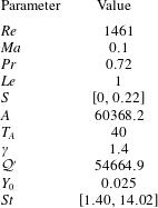
In the derivation of these equations (Poinsot & Veynante Reference Poinsot and Veynante2012), the dimensional variables, denoted with a hat, have been rendered non-dimensional using the reference quantities listed in table 1. This scaling produces five dimensionless parameters, also listed in table 1, that govern the flow, acoustics and reaction dynamics.
Definitions of the non-dimensional variables and parameters. The reference temperature
 $T_{0}$
, density
 $\unicode[STIX]{x1D70C}_{0}$
, velocity
 $U$
and mass fractions
 $Y_{0}$
stem from the values of the fresh gas in the inlet tube. Even though the mass fraction
 ${\hat{Y}}$
is already non-dimensional, dividing by the values in the fresh gases ensures that the new variable
 $Y$
ranges from one in the fresh gases to zero in the burnt gases. The constant
 $C_{P}$
denotes the heat capacity at constant pressure,
 $\unicode[STIX]{x1D707}$
represents the dynamic viscosity,
 $\unicode[STIX]{x1D706}$
is the thermal conductivity and
 $D$
stands for the diffusion coefficient. The radii
 $r_{in}$
and
 $r_{out}$
in the swirl number definition are the non-dimensional inner and outer radii of the inlet annulus, respectively.

Equations (2.1) and (2.2) represent conservation of mass and momentum, respectively. Owing to compressibility, we require an energy equation (2.3) which we take to be an equation for the total non-chemical energy,
 $$\begin{eqnarray}E={\displaystyle \frac{1}{2}}\boldsymbol{u}\boldsymbol{\cdot }\boldsymbol{u}+{\displaystyle \frac{P}{\unicode[STIX]{x1D70C}(\unicode[STIX]{x1D6FE}-1)}},\end{eqnarray}$$
given by the sum of the kinetic and internal energies per unit mass. The constant
 ${\mathcal{Q}}^{\prime }$
in (2.3) is the heat release per unit mass of fuel. The fuel mass fraction
 $Y$
evolves according to (2.4), and the reaction rate is explicitly given through an Arrhenius law
 $$\begin{eqnarray}\dot{\unicode[STIX]{x1D714}}_{f}=A\unicode[STIX]{x1D70C}Y_{0}Y\exp (-T_{a}/T),\end{eqnarray}$$
where
 $T_{a}$
is the activation temperature and
 $A$
is the Arrhenius constant.
In order to obtain the equations in this form, several assumptions had to be made. The reaction is taken to be very lean, hence only the fuel mass fraction
 $Y$
is required when calculating the reaction rate. The heat capacities of all species are assumed to be identical, and the gas is taken to be perfect, which establishes a relation between the pressure and the temperature. In our non-dimensional variables, this relation reads
 $$\begin{eqnarray}P={\displaystyle \frac{\unicode[STIX]{x1D70C}T}{\unicode[STIX]{x1D6FE}Ma^{2}}}.\end{eqnarray}$$
We further assume that the heat capacities, the Prandtl number and the Lewis number are constants with respect to temperature, but we allow the Reynolds number to vary according to Sutherland’s law for the viscosity (Sutherland Reference Sutherland1893). The diffusion coefficients of both species are taken to be equal, allowing us to use Fick’s law (Fick Reference Fick1995) to simplify the diffusion velocities in (2.4).
2.2 Numerical details
The numerical implementation of the above governing equations follows the outline given in Garnaud (Reference Garnaud2012) and Blanchard (Reference Blanchard2015), but is augmented to allow for swirling flows and three-dimensionality (non-zero azimuthal wavenumbers) in the linearised equations. It uses higher-order upwinded low-dissipation explicit schemes for the spatial derivatives (Berland et al. Reference Berland, Bogey, Marsden and Bailly2007), Krylov subspace time stepping and a zonal domain decomposition technique for parallelising the calculations.
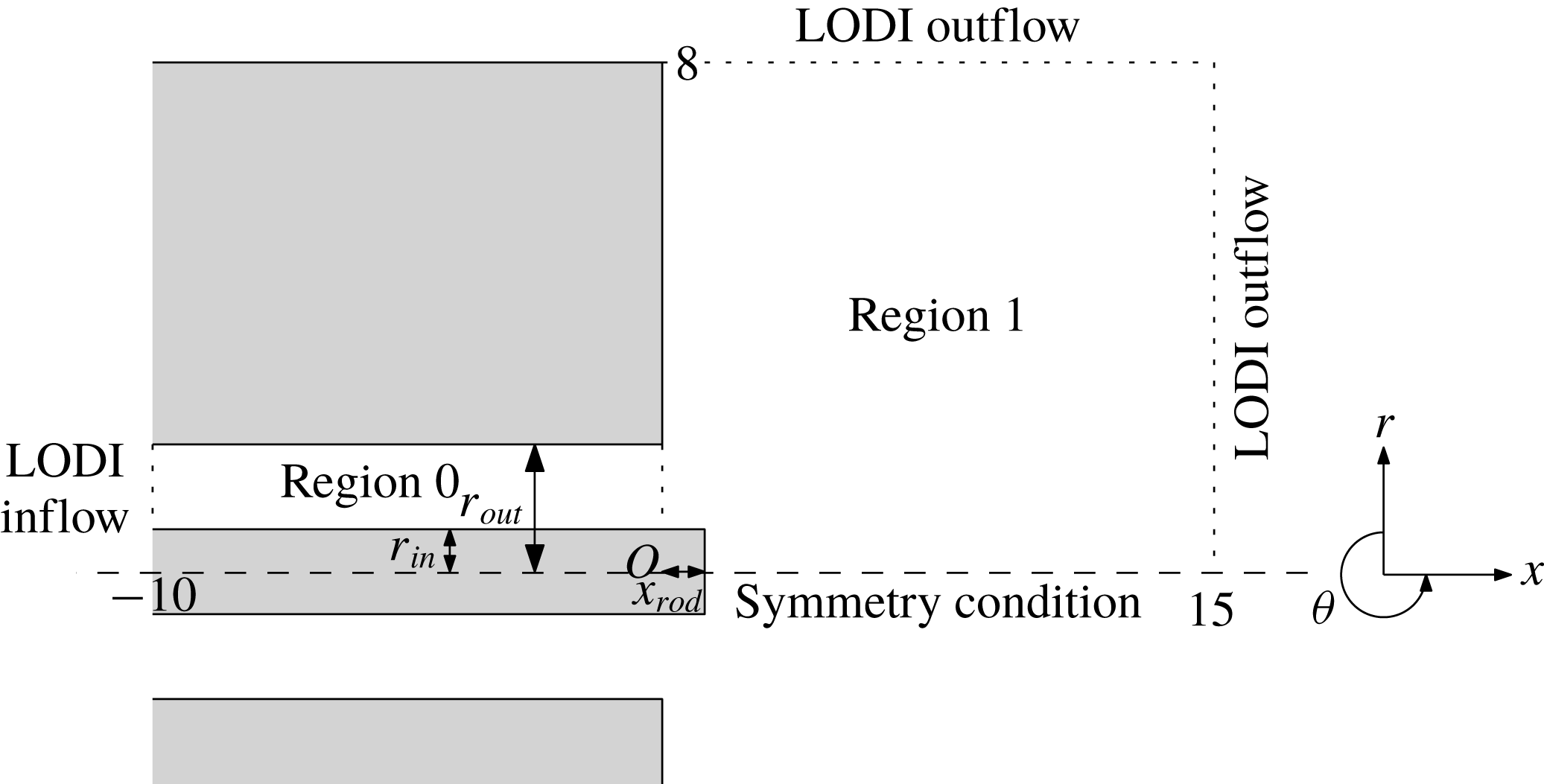
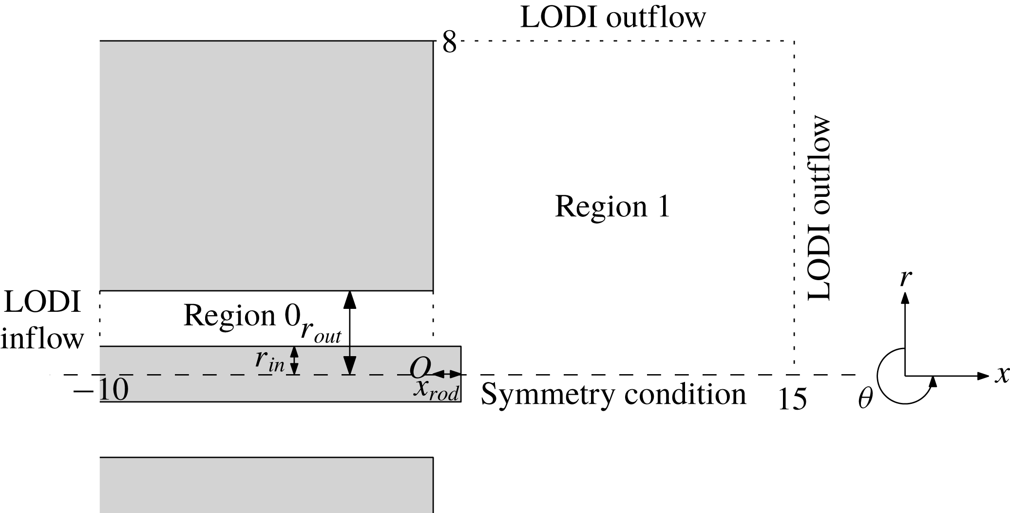
Figure 1 shows the numerical domain, which is divided into two distinct subregions. Region
 $0$
consists of an inlet annulus through which fresh gases propagate to region
 $1$
, a cylindrical combustion chamber. The central rod has radius
 $r_{in}$
and protrudes into region 1 by an amount
 $x_{rod}$
. The outer boundary of the inlet tube is at
 $r=r_{out}$
. Owing to the nature of the geometry, cylindrical polar coordinates are used, adopting the formulation given by Sandberg (Reference Sandberg2007).
For simplicity we recast the non-dimensional governing equations into
 $$\begin{eqnarray}{\displaystyle \frac{\unicode[STIX]{x2202}\boldsymbol{q}}{\unicode[STIX]{x2202}t}}=\boldsymbol{{\mathcal{N}}}(\boldsymbol{q}),\end{eqnarray}$$
where
 $\boldsymbol{{\mathcal{N}}}$
represents the right-hand side of (2.1)–(2.4) in conservative form, and the state
 $\boldsymbol{q}$
consists of the dynamic quantities
 $(\unicode[STIX]{x1D70C},\unicode[STIX]{x1D70C}u_{x},\unicode[STIX]{x1D70C}u_{r},\unicode[STIX]{x1D70C}u_{\unicode[STIX]{x1D703}},\unicode[STIX]{x1D70C}E,\unicode[STIX]{x1D70C}Y)^{\text{T}}$
. Locally one-dimensional inviscid (LODI) boundary conditions (Poinsot & Lele Reference Poinsot and Lele1992) are used for an inflow boundary condition in region
 $0$
, where fresh gases are being injected, and as an outflow condition in region
 $1$
to ensure an open combustion area with minimal wave reflections from the computational boundary. The absence of wave reflections has been checked by varying the downstream boundaries by one non-dimensional unit and recalculating the optimal gain for
 $S=0,~m=0,~\mathit{St}=4.21$
: a relative change in the optimal gain by
 ${\approx}0.1\,\%$
has been found, demonstrating that wave reflection from the edge of the computational domain does not significantly impact our analysis.
Sketch of the computational domain consisting of an annular inflow region (region
 $0$
) and an open combustion region (region
 $1$
). LODI boundary conditions are used at the inlet and the open boundaries of region
 $1$
.
A nonlinear solver determines an equilibrium solution to the axisymmetric version of (2.8), i.e. with
 $\unicode[STIX]{x2202}_{\unicode[STIX]{x1D703}}\equiv 0$
. During this solution process, selective frequency damping (Åkervik et al.
Reference Åkervik, Brandt, Henningson, Hœpffner, Marxen and Schlatter2006) is used for convergence acceleration. We denote these axisymmetric base-flow solutions by
 $\boldsymbol{q}_{0}$
with
 $\boldsymbol{{\mathcal{N}}}(\boldsymbol{q}_{0})=0$
. Based on these equilibrium states, we investigate the linear dynamics of swirling flames by considering perturbations about
 $\boldsymbol{q}_{0}$
. To this end, we linearise the nonlinear operator
 $\boldsymbol{{\mathcal{N}}}(\boldsymbol{q})$
about the base flow
 $\boldsymbol{q}_{0}$
to find the governing linear operator.
While the base flow is taken as axisymmetric, we allow for non-axisymmetric disturbances by considering flow fields of the form
 $\boldsymbol{q}(t,x,r,\unicode[STIX]{x1D703})=\boldsymbol{q}_{0}(x,r)+\boldsymbol{q}^{\prime }(t,x,r)\text{e}^{\text{i}m\unicode[STIX]{x1D703}}$
, where we have Fourier-transformed the linear variable
 $\boldsymbol{q}^{\prime }$
in the
 $\unicode[STIX]{x1D703}$
direction, introducing the integer azimuthal wavenumber
 $m$
. The full linear (discretised) operator
 $\unicode[STIX]{x1D63C}$
is given by
 $$\begin{eqnarray}\left.{\displaystyle \frac{\unicode[STIX]{x2202}\boldsymbol{{\mathcal{N}}}(\boldsymbol{q})}{\unicode[STIX]{x2202}\boldsymbol{q}}}\right|_{\boldsymbol{q}=\boldsymbol{q}_{0}}(\boldsymbol{q}^{\prime }\text{e}^{\text{i}m\unicode[STIX]{x1D703}})=\unicode[STIX]{x1D63C}(\boldsymbol{q}^{\prime }\text{e}^{\text{i}m\unicode[STIX]{x1D703}}).\end{eqnarray}$$
It will prove useful to instead consider the linear operator for azimuthal mode
 $m$
directly by writing
 $\unicode[STIX]{x1D63C}(\boldsymbol{q}^{\prime }\text{e}^{\text{i}m\unicode[STIX]{x1D703}})=\text{e}^{\text{i}m\unicode[STIX]{x1D703}}\unicode[STIX]{x1D63C}_{m}\boldsymbol{q}^{\prime }$
, i.e.
 $\unicode[STIX]{x1D63C}_{m}$
stands for the linear operator with azimuthal
 $\unicode[STIX]{x1D703}$
derivatives replaced by
 $\text{i}m$
multiplications. For our subsequent analysis, the linear operator adjoint to
 $\unicode[STIX]{x1D63C}_{m}$
is required. This latter operator
 $\unicode[STIX]{x1D63C}_{m}^{\text{H}}$
and the direct operator
 $\unicode[STIX]{x1D63C}_{m}$
are not explicitly formed (nor derived), but are rather defined by their action on respective flow fields via an automatic differentiation approach directly applied to the nonlinear routines; see Fosas de Pando, Sipp & Schmid (Reference Fosas de Pando, Sipp and Schmid2012) for details. The resulting operator
 $\unicode[STIX]{x1D63C}_{m}$
has been checked to be consistent with the nonlinear operator by a finite-difference scheme.
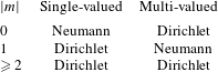
The centreline boundary conditions for single-valued and multi-valued quantities for different azimuthal wavenumbers
 $m$
.
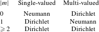
An important component in the linearised equations for each azimuthal mode is in the centreline boundary condition. In region
 $1$
at
 $r=0$
, the numerical implementation encounters a coordinate singularity. To correctly attend to this singularity, a staggered mesh is employed, thus avoiding a grid point directly at
 $r=0$
. Radial derivatives near
 $r=0$
are then evaluated by enforcing a symmetry condition across the centreline (Mohseni & Colonius Reference Mohseni and Colonius2000). The form of this symmetry condition is dependent on the azimuthal wavenumber
 $m$
under consideration (Constantinescu & Lele Reference Constantinescu and Lele2002). At the centreline, state variables fall into two categories: single-valued variables such as
 $\unicode[STIX]{x1D70C}$
,
 $u_{x}$
,
 $Y$
and
 $E$
, and multi-valued quantities such as
 $u_{r}$
and
 $u_{\unicode[STIX]{x1D703}}$
. The correct symmetry conditions for the continuation of these variables across the centreline are given in table 2.
2.3 Numerical optimal gains
The analysis of the swirling M-flame revolves around the concept of a frequency response or transfer function. To this end, we harmonically perturb the governing equations with a small force
 $\unicode[STIX]{x1D716}\,\boldsymbol{f}(x,r)$
(
 $\unicode[STIX]{x1D716}\ll 0$
) at an azimuthal wavenumber
 $m$
and temporal frequency
 $\unicode[STIX]{x1D714}$
,
 $$\begin{eqnarray}{\displaystyle \frac{\unicode[STIX]{x2202}\boldsymbol{q}}{\unicode[STIX]{x2202}t}}=\boldsymbol{{\mathcal{N}}}(\boldsymbol{q})+\unicode[STIX]{x1D716}\,\boldsymbol{f}_{m,\unicode[STIX]{x1D714}}\text{e}^{\text{i}m\unicode[STIX]{x1D703}}\text{e}^{\text{i}\unicode[STIX]{x1D714}t},\end{eqnarray}$$
and seek solutions in the form
 $\boldsymbol{q}(t,x,r,\unicode[STIX]{x1D703})=\boldsymbol{q}_{0}(x,r)+\boldsymbol{q}_{m}^{\prime }(t,x,r)\text{e}^{\text{i}m\unicode[STIX]{x1D703}}$
. Substituting this expression into (2.10) and separating out orders in
 $\unicode[STIX]{x1D716}$
, we obtain for the first two orders (
 $\unicode[STIX]{x1D716}^{0}$
and
 $\unicode[STIX]{x1D716}^{1}$
)
 $$\begin{eqnarray}\displaystyle \boldsymbol{{\mathcal{N}}}(\boldsymbol{q}_{0}) & = & \displaystyle 0,\end{eqnarray}$$
 $$\begin{eqnarray}\displaystyle {\displaystyle \frac{\unicode[STIX]{x2202}\boldsymbol{q}_{m}^{\prime }}{\unicode[STIX]{x2202}t}} & = & \displaystyle \unicode[STIX]{x1D63C}_{m}\boldsymbol{q}_{m}^{\prime }+\boldsymbol{f}_{m,\unicode[STIX]{x1D714}}\text{e}^{\text{i}\unicode[STIX]{x1D714}t}.\end{eqnarray}$$
 $\boldsymbol{q}_{0}$
to be a steady solution of the nonlinear governing equations, while (2.11b
) represents the forced, linear equations of motion for a perturbation at wavenumber
 $m$
. For stable
 $\unicode[STIX]{x1D63C}_{m}$
, we obtain bounded solutions, and, due to the linearity of the problem, the perturbation
 $\boldsymbol{q}_{m}^{\prime }$
will eventually respond at the forcing frequency
 $\unicode[STIX]{x1D714}$
. We hence can write
 $\boldsymbol{q}_{m}^{\prime }(t,x,r)=\bar{\boldsymbol{q}}_{m}(t,x,r)\text{e}^{\text{i}\unicode[STIX]{x1D714}t}$
, where we use the time-dependent variable
 $\bar{\boldsymbol{q}}_{m}$
to denote the driven response including transient effects. The long-time driven response (after transient effects have subsided) in
 $\boldsymbol{q}_{m,\unicode[STIX]{x1D714}}(x,r)=\bar{\boldsymbol{q}}_{m}(t\rightarrow \infty ,x,r)$
is determined as the steady solution of
 $$\begin{eqnarray}{\displaystyle \frac{\unicode[STIX]{x2202}\bar{\boldsymbol{q}}_{m}}{\unicode[STIX]{x2202}t}}+\text{i}\unicode[STIX]{x1D714}\bar{\boldsymbol{q}}_{m}=\unicode[STIX]{x1D63C}_{m}\bar{\boldsymbol{q}}_{m}+\boldsymbol{f}_{m,\unicode[STIX]{x1D714}},\end{eqnarray}$$
which is obtained by substituting the above expression for
 $\boldsymbol{q}_{m}^{\prime }$
into (2.11b
) and cancelling the exponential terms. Equation (2.12) presents a concise and computationally efficient way to obtain the driven response
 $\boldsymbol{q}_{m,\unicode[STIX]{x1D714}}(x,r)=\unicode[STIX]{x1D64D}_{m,\unicode[STIX]{x1D714}}\,\boldsymbol{f}_{m,\unicode[STIX]{x1D714}}$
given by the resolvent matrix
 $\unicode[STIX]{x1D64D}_{m,\unicode[STIX]{x1D714}}=(\text{i}\unicode[STIX]{x1D714}\unicode[STIX]{x1D644}-\unicode[STIX]{x1D63C}_{m})^{-1}$
.
The resolvent represents the transfer function that links a forcing shape
 $\boldsymbol{f}_{m,\unicode[STIX]{x1D714}}$
to its driven response
 $\boldsymbol{q}_{m,\unicode[STIX]{x1D714}}$
at frequency
 $\unicode[STIX]{x1D714}$
. We could choose a specific forcing shape and investigate the corresponding output and gain, defined as
 $\unicode[STIX]{x1D70E}_{m,\unicode[STIX]{x1D714}}=\Vert \boldsymbol{q}_{m,\unicode[STIX]{x1D714}}\Vert /\Vert \,\boldsymbol{f}_{m,\unicode[STIX]{x1D714}}\Vert$
for some norm
 $\Vert \cdot \Vert$
, but instead we seek the forcing that maximises the gain for a given frequency. In this manner, not only do we obtain the maximum possible gain for our system, but also, by investigating the structures of the forcing and output, we gain insight into dominant mechanisms that underly this amplification and exploit various processes (of hydrodynamic, acoustic, reactive type, or a combination thereof) within the full system.
For a measure of disturbance size, we choose the Chu norm (Chu Reference Chu1965), a compressible energy-based norm, and modify it to include reactive terms (see Blanchard Reference Blanchard2015). We have
 $$\begin{eqnarray}\Vert \boldsymbol{q}\Vert ^{2}={\displaystyle \frac{1}{2\unicode[STIX]{x03C0}}}\iiint _{\unicode[STIX]{x1D6FA}}\left[\unicode[STIX]{x1D70C}_{0}|\boldsymbol{u}^{\prime }|^{2}+{\displaystyle \frac{P_{0}|\unicode[STIX]{x1D70C}^{\prime }|^{2}}{\unicode[STIX]{x1D70C}_{0}^{2}}}+{\displaystyle \frac{\unicode[STIX]{x1D70C}_{0}^{2}(|T^{\prime }|^{2}+|Q^{\prime }Ma^{2}(\unicode[STIX]{x1D6FE}-1)Y_{0}Y^{\prime }|^{2})}{\unicode[STIX]{x1D6FE}^{2}(\unicode[STIX]{x1D6FE}-1)Ma^{4}P_{0}}}\right]\text{d}V,\end{eqnarray}$$
with
 $\text{d}V=r\,\text{d}r\,\text{d}x\,\text{d}\unicode[STIX]{x1D703}$
. Choosing an appropriate norm is a crucial step in our analysis, since all computed gains are dependent on this choice. By selecting a physically motivated norm, we ensure that we obtain physically relevant forcings and thus uncover pertinent mechanisms that describe the overall flame behaviour. The Chu norm, in the form given by (2.13), will allow us to compute the optimal gain by accounting for hydrodynamic, acoustic, thermal or reactive effects, without biasing towards any.
By translating the norm (2.13) into a corresponding weight matrix
 $\unicode[STIX]{x1D652}$
, we can define our discrete norm
 $\Vert \cdot \Vert$
as the norm induced by the inner product
 $\langle \boldsymbol{x},\boldsymbol{y}\rangle _{\unicode[STIX]{x1D652}}=\boldsymbol{x}^{\text{H}}\unicode[STIX]{x1D652}\boldsymbol{y}$
. We then link this norm to the standard vector
 $2$
-norm by employing a Cholesky decomposition of
 $\unicode[STIX]{x1D652}=\unicode[STIX]{x1D648}^{\text{H}}\unicode[STIX]{x1D648}$
. Our optimal gain problem can then be stated as finding the forcing given by
 $$\begin{eqnarray}\boldsymbol{f}_{m,\unicode[STIX]{x1D714}}^{opt}=\underset{\boldsymbol{f}_{m,\unicode[STIX]{x1D714}}}{\text{arg max}}{\displaystyle \frac{\Vert \unicode[STIX]{x1D648}\unicode[STIX]{x1D647}_{out}\boldsymbol{R}_{m,\unicode[STIX]{x1D714}}\unicode[STIX]{x1D647}_{in}\unicode[STIX]{x1D648}^{-1}\unicode[STIX]{x1D648}\,\boldsymbol{f}_{m,\unicode[STIX]{x1D714}}\Vert _{2}}{\Vert \unicode[STIX]{x1D648}\,\boldsymbol{f}_{m,\unicode[STIX]{x1D714}}\Vert _{2}}}.\end{eqnarray}$$
In the expression above, we have additionally introduced two windowing matrices
 $\unicode[STIX]{x1D647}_{out}$
and
 $\unicode[STIX]{x1D647}_{in}$
. These matrices act as masks to select (or deselect) specific regions of the computational domain or variables of interest for our forcing and output. For our case, we restrict the forcing to the region in the inlet tube with
 $-2.5\leqslant x\leqslant -0.5$
. The associated response will be confined to the burning area (
 $x>0$
) by appropriately choosing
 $\boldsymbol{L}_{out}$
. The solution to the above optimisation is obtained by the SVD as follows: the principal singular triplet of
 $\unicode[STIX]{x1D648}\boldsymbol{L}_{out}\boldsymbol{R}_{m,\unicode[STIX]{x1D714}}\boldsymbol{L}_{in}\unicode[STIX]{x1D648}^{-1}$
is
 $(\unicode[STIX]{x1D70E}_{m,\unicode[STIX]{x1D714}},\unicode[STIX]{x1D648}\boldsymbol{q}_{m,\unicode[STIX]{x1D714}}^{opt},\unicode[STIX]{x1D648}\,\boldsymbol{f}_{m,\unicode[STIX]{x1D714}}^{opt})$
, giving the optimal forced response as
 $\tilde{\boldsymbol{q}}_{m,\unicode[STIX]{x1D714}}^{opt}=\unicode[STIX]{x1D70E}_{m,\unicode[STIX]{x1D714}}\boldsymbol{q}_{m,\unicode[STIX]{x1D714}}^{opt}$
.
While the above expressions furnish a procedure to analyse the linear dynamics of the swirling M-flame, the computational steps to obtain the resolvent operator and the SVD are prohibitively expensive due to the many degrees of freedom in our discretised system. Instead, we approximate the multiplication of the discrete resolvent matrix with an arbitrary state vector
 $\boldsymbol{x}$
by the long-time integration of (2.12) with the forcing
 $\boldsymbol{f}_{m,\unicode[STIX]{x1D714}}=\boldsymbol{x}$
(and the initial condition
 $\boldsymbol{q}_{m}=0$
). Likewise, the action of the adjoint resolvent matrix on an adjoint state vector
 $\boldsymbol{x}^{\dagger }$
is given by the
 $\bar{\boldsymbol{f}}_{m}^{\dagger }$
component of the long-time integration of the adjoint equation to (2.12), given by
 $$\begin{eqnarray}\displaystyle & \displaystyle {\displaystyle \frac{\unicode[STIX]{x2202}\bar{\boldsymbol{q}}_{m}^{\dagger }}{\unicode[STIX]{x2202}t}}-\text{i}\unicode[STIX]{x1D714}\bar{\boldsymbol{q}}_{m}^{\dagger }=\unicode[STIX]{x1D63C}_{m}^{\text{H}}\bar{\boldsymbol{q}}_{m}^{\dagger }, & \displaystyle\end{eqnarray}$$
 $$\begin{eqnarray}\displaystyle & \displaystyle \frac{\unicode[STIX]{x2202}\bar{\boldsymbol{f}}_{m}^{\dagger }}{\unicode[STIX]{x2202}t}=\bar{\boldsymbol{q}}_{m}^{\dagger }, & \displaystyle\end{eqnarray}$$
 $\bar{\boldsymbol{q}}_{m}^{\dagger }(0)=\boldsymbol{x}^{\dagger }$
,
 $\bar{\boldsymbol{f}}_{m}^{\dagger }(0)=0$
. The time horizon
 $T$
for these integrations must be sufficiently large to ensure convergence to a steady solution, but reasonably small to keep simulation times within a feasible range. A final time of
 $T=10$
has been found to achieve this compromise.
2.4 Numerical sensitivity analysis
The computation of optimal gains using the direct–adjoint framework presented above, which is equivalent to evaluating the SVD of the resolvent operator, requires a substantial amount of resources. This means that, realistically, only a small number of frequencies can be calculated.
Moreover, one has to keep in mind that all computed gains are parameter-dependent, and, in order to assess the variation of preferred amplification behaviour with changes in one of the governing parameters (recall table 1), many more computations would be necessary. It is thus very important to extract a maximum of information from each calculation, to leverage direct and adjoint solutions, and to fully harness the expended computational effort. To this end, we will formulate a sensitivity-based technique to approximate variations in the frequency response (resolvent norm) with respect to changes in any parameter. This formulation stems from the realisation that adjoint variables are generalised sensitivities or gradients, and expressions for parametric sensitivities can be given in terms of weighted scalar products between the direct and adjoint solutions.
The underlying principle behind the parametric sensitivities is a first-order perturbation approach applied to the SVD with respect to the linearised operator (Fosas de Pando et al. Reference Fosas de Pando, Schmid and Lele2014). We generally have
 $$\begin{eqnarray}\unicode[STIX]{x1D6FF}\unicode[STIX]{x1D70E}=Re[\boldsymbol{u}^{\text{H}}\unicode[STIX]{x1D6FF}\unicode[STIX]{x1D646}\boldsymbol{v}],\end{eqnarray}$$
which relates first-order changes in the maximal singular value
 $\unicode[STIX]{x1D70E}$
(in our case, the optimal gain) to first-order changes in the underlying matrix
 $\unicode[STIX]{x1D646}$
, where
 $(\unicode[STIX]{x1D70E},\boldsymbol{u},\boldsymbol{v})$
stands for the principal singular triplet of
 $\unicode[STIX]{x1D646}$
. Using this relation with
 $\unicode[STIX]{x1D646}=\unicode[STIX]{x1D648}\unicode[STIX]{x1D647}_{out}\unicode[STIX]{x1D64D}_{m,\unicode[STIX]{x1D714}}\unicode[STIX]{x1D647}_{in}\unicode[STIX]{x1D648}^{-1}$
, we can derive the sensitivity with respect to, for example, the forcing frequency
 $\unicode[STIX]{x1D714}$
according to
 $$\begin{eqnarray}\displaystyle {\displaystyle \frac{\unicode[STIX]{x2202}\unicode[STIX]{x1D70E}_{m,\unicode[STIX]{x1D714}}}{\unicode[STIX]{x2202}\unicode[STIX]{x1D714}}} & = & \displaystyle Im[\langle \boldsymbol{q}_{m,\unicode[STIX]{x1D714}}^{opt},\unicode[STIX]{x1D647}_{out}\unicode[STIX]{x1D64D}_{m,\unicode[STIX]{x1D714}}\unicode[STIX]{x1D64D}_{m,\unicode[STIX]{x1D714}}\unicode[STIX]{x1D647}_{in}\,\boldsymbol{f}_{m,\unicode[STIX]{x1D714}}^{opt}\rangle _{\unicode[STIX]{x1D652}}].\end{eqnarray}$$
This simplified expression results from the fact that the frequency
 $\unicode[STIX]{x1D714}$
appears linearly and isolated from the linearised operator
 $\unicode[STIX]{x1D63C}_{m}$
.
To evaluate the sensitivity with respect to other parameters, representatively denoted by
 $\unicode[STIX]{x1D6FC}$
, we use the product rule to obtain
 $$\begin{eqnarray}\displaystyle {\displaystyle \frac{\unicode[STIX]{x2202}\unicode[STIX]{x1D70E}_{m,\unicode[STIX]{x1D714}}}{\unicode[STIX]{x2202}\unicode[STIX]{x1D6FC}}} & = & \displaystyle Re\left[\left\langle \boldsymbol{q}_{m,\unicode[STIX]{x1D714}}^{opt},\unicode[STIX]{x1D647}_{out}\unicode[STIX]{x1D64D}_{m,\unicode[STIX]{x1D714}}{\displaystyle \frac{\unicode[STIX]{x2202}\unicode[STIX]{x1D63C}_{m}}{\unicode[STIX]{x2202}\unicode[STIX]{x1D6FC}}}\unicode[STIX]{x1D64D}_{m,\unicode[STIX]{x1D714}}\unicode[STIX]{x1D647}_{in}\,\boldsymbol{f}_{m,\unicode[STIX]{x1D714}}^{opt}\right\rangle _{\!\unicode[STIX]{x1D652}}\right]\nonumber\\ \displaystyle & & \displaystyle +\,\unicode[STIX]{x1D70E}_{m,\unicode[STIX]{x1D714}}\,Re\left[\left\langle \unicode[STIX]{x1D648}\boldsymbol{q}_{m,\unicode[STIX]{x1D714}}^{opt},{\displaystyle \frac{\unicode[STIX]{x2202}\unicode[STIX]{x1D648}}{\unicode[STIX]{x2202}\unicode[STIX]{x1D6FC}}}\boldsymbol{q}_{m,\unicode[STIX]{x1D714}}^{opt}\right\rangle \right]\nonumber\\ \displaystyle & & \displaystyle -\,Re\left[\left\langle \boldsymbol{q}_{m,\unicode[STIX]{x1D714}}^{opt},\unicode[STIX]{x1D647}_{out}\unicode[STIX]{x1D64D}_{m,\unicode[STIX]{x1D714}}\unicode[STIX]{x1D647}_{in}\unicode[STIX]{x1D648}^{-1}{\displaystyle \frac{\unicode[STIX]{x2202}\unicode[STIX]{x1D648}}{\unicode[STIX]{x2202}\unicode[STIX]{x1D6FC}}}\,\boldsymbol{f}_{m,\unicode[STIX]{x1D714}}^{opt}\right\rangle _{\!\unicode[STIX]{x1D652}}\right].\end{eqnarray}$$
Equation (2.17) indicates that two resolvent calculations are required to determine the sensitivity with respect to the forcing frequency, while (2.18) shows that three resolvent calculations are sufficient to obtain the sensitivity with respect to each parameter. However, by first calculating the two quantities
 $$\begin{eqnarray}\unicode[STIX]{x1D753}_{m,\unicode[STIX]{x1D714}}^{\,f}=\unicode[STIX]{x1D64D}_{m,\unicode[STIX]{x1D714}}\unicode[STIX]{x1D647}_{in}\,\boldsymbol{f}_{m,\unicode[STIX]{x1D714}}^{opt},\quad \unicode[STIX]{x1D753}_{m,\unicode[STIX]{x1D714}}^{q}=\unicode[STIX]{x1D64D}_{m,\unicode[STIX]{x1D714}}^{\text{H}}\unicode[STIX]{x1D647}_{out}^{\text{H}}\unicode[STIX]{x1D652}^{\text{H}}\boldsymbol{q}_{m,\unicode[STIX]{x1D714}}^{opt},\end{eqnarray}$$
followed by rewriting the above sensitivities (2.17) and (2.18) in the form
 $$\begin{eqnarray}\displaystyle {\displaystyle \frac{\unicode[STIX]{x2202}\unicode[STIX]{x1D70E}_{m,\unicode[STIX]{x1D714}}}{\unicode[STIX]{x2202}\unicode[STIX]{x1D714}}} & = & \displaystyle Im[\langle \unicode[STIX]{x1D753}_{m,\unicode[STIX]{x1D714}}^{q},\unicode[STIX]{x1D753}_{m,\unicode[STIX]{x1D714}}^{\,f}\rangle ],\end{eqnarray}$$
 $$\begin{eqnarray}\displaystyle {\displaystyle \frac{\unicode[STIX]{x2202}\unicode[STIX]{x1D70E}_{m,\unicode[STIX]{x1D714}}}{\unicode[STIX]{x2202}\unicode[STIX]{x1D6FC}}} & = & \displaystyle Re\left[\left\langle \unicode[STIX]{x1D753}_{m,\unicode[STIX]{x1D714}}^{q},{\displaystyle \frac{\unicode[STIX]{x2202}\unicode[STIX]{x1D63C}_{m}}{\unicode[STIX]{x2202}\unicode[STIX]{x1D6FC}}}\unicode[STIX]{x1D753}_{m,\unicode[STIX]{x1D714}}^{\,f}\right\rangle \right]\nonumber\\ \displaystyle & & \displaystyle +\,\unicode[STIX]{x1D70E}_{m,\unicode[STIX]{x1D714}}\,Re\left[\left\langle \unicode[STIX]{x1D648}\boldsymbol{q}_{m,\unicode[STIX]{x1D714}}^{opt},{\displaystyle \frac{\unicode[STIX]{x2202}\unicode[STIX]{x1D648}}{\unicode[STIX]{x2202}\unicode[STIX]{x1D6FC}}}\boldsymbol{q}_{m,\unicode[STIX]{x1D714}}^{opt}\right\rangle \right]\nonumber\\ \displaystyle & & \displaystyle -\,Re\left[\left\langle \unicode[STIX]{x1D753}_{m,\unicode[STIX]{x1D714}}^{q},\unicode[STIX]{x1D647}_{in}\unicode[STIX]{x1D648}^{-1}{\displaystyle \frac{\unicode[STIX]{x2202}\unicode[STIX]{x1D648}}{\unicode[STIX]{x2202}\unicode[STIX]{x1D6FC}}}\,\boldsymbol{f}_{m,\unicode[STIX]{x1D714}}^{opt}\right\rangle \right]\!,\end{eqnarray}$$
we can reduce the number of resolvent calculations to just two for the sensitivity with respect to any parameter, namely the resolvent calculations contained in
 $\unicode[STIX]{x1D753}_{m,\unicode[STIX]{x1D714}}^{\,f}$
and
 $\unicode[STIX]{x1D753}_{m,\unicode[STIX]{x1D714}}^{q}$
. We identify the three terms of (2.21) as the variation in singular value
 $\unicode[STIX]{x1D70E}_{m,\unicode[STIX]{x1D714}}$
due to changes in (i) the governing linear operator, (ii) the norm of the output and (iii) the norm of the input, respectively.
The derivatives of
 $\unicode[STIX]{x1D63C}_{m}$
and
 $\unicode[STIX]{x1D648}$
are approximated by simple first-order finite differences according to
 $$\begin{eqnarray}{\displaystyle \frac{\unicode[STIX]{x2202}\unicode[STIX]{x1D63C}_{m}}{\unicode[STIX]{x2202}\unicode[STIX]{x1D6FC}}}={\displaystyle \frac{\unicode[STIX]{x1D63C}_{m}(\unicode[STIX]{x1D6FC}+\unicode[STIX]{x1D716})-\unicode[STIX]{x1D63C}_{m}(\unicode[STIX]{x1D6FC})}{\unicode[STIX]{x1D716}}},\quad {\displaystyle \frac{\unicode[STIX]{x2202}\unicode[STIX]{x1D648}}{\unicode[STIX]{x2202}\unicode[STIX]{x1D6FC}}}={\displaystyle \frac{\unicode[STIX]{x1D648}(\unicode[STIX]{x1D6FC}+\unicode[STIX]{x1D716})-\unicode[STIX]{x1D648}(\unicode[STIX]{x1D6FC})}{\unicode[STIX]{x1D716}}}.\end{eqnarray}$$
In the case where the two windowing matrices overlap, i.e. the product
 $\unicode[STIX]{x1D647}_{in}\unicode[STIX]{x1D647}_{out}\neq 0$
, we can attain all these sensitivities with no resolvent calculations, simply by perturbing the smallest singular value of the pseudo-inverse of
 $\unicode[STIX]{x1D646}$
, given by
 $\unicode[STIX]{x1D646}^{+}=\unicode[STIX]{x1D648}\unicode[STIX]{x1D647}_{in}^{\text{H}}\unicode[STIX]{x1D64D}_{m,\unicode[STIX]{x1D714}}^{-1}\unicode[STIX]{x1D647}_{out}^{\text{H}}\unicode[STIX]{x1D648}^{-1}$
. The relation
 $$\begin{eqnarray}\unicode[STIX]{x1D6FF}\left({\displaystyle \frac{1}{\unicode[STIX]{x1D70E}}}\right)=Re[\boldsymbol{v}^{\text{H}}\unicode[STIX]{x1D6FF}\unicode[STIX]{x1D646}^{+}\boldsymbol{u}]\end{eqnarray}$$
provides us with the formulae
 $$\begin{eqnarray}\displaystyle {\displaystyle \frac{1}{\unicode[STIX]{x1D70E}_{m,\unicode[STIX]{x1D714}}^{2}}}{\displaystyle \frac{\unicode[STIX]{x2202}\unicode[STIX]{x1D70E}_{m,\unicode[STIX]{x1D714}}}{\unicode[STIX]{x2202}\unicode[STIX]{x1D714}}} & = & \displaystyle Im[\langle \,\boldsymbol{f}_{m,\unicode[STIX]{x1D714}}^{opt},\unicode[STIX]{x1D647}_{in}^{\text{H}}\unicode[STIX]{x1D647}_{out}^{\text{H}}\boldsymbol{q}_{m,\unicode[STIX]{x1D714}}^{opt}\rangle _{\unicode[STIX]{x1D652}}],\end{eqnarray}$$
 $$\begin{eqnarray}\displaystyle {\displaystyle \frac{1}{\unicode[STIX]{x1D70E}_{m,\unicode[STIX]{x1D714}}^{2}}}{\displaystyle \frac{\unicode[STIX]{x2202}\unicode[STIX]{x1D70E}_{m,\unicode[STIX]{x1D714}}}{\unicode[STIX]{x2202}\unicode[STIX]{x1D6FC}}} & = & \displaystyle Re\left[\left\langle \,\boldsymbol{f}_{m,\unicode[STIX]{x1D714}}^{opt},\unicode[STIX]{x1D647}_{in}^{\text{H}}{\displaystyle \frac{\unicode[STIX]{x2202}\unicode[STIX]{x1D63C}_{m}}{\unicode[STIX]{x2202}\unicode[STIX]{x1D6FC}}}\unicode[STIX]{x1D647}_{out}^{\text{H}}\boldsymbol{q}_{m,\unicode[STIX]{x1D714}}^{opt}\right\rangle _{\!\unicode[STIX]{x1D652}}\right]\nonumber\\ \displaystyle & & \displaystyle -\,\frac{1}{\unicode[STIX]{x1D70E}_{m,\unicode[STIX]{x1D714}}}Re\left[\left\langle \unicode[STIX]{x1D648}\,\boldsymbol{f}_{m,\unicode[STIX]{x1D714}}^{opt},{\displaystyle \frac{\unicode[STIX]{x2202}\unicode[STIX]{x1D648}}{\unicode[STIX]{x2202}\unicode[STIX]{x1D6FC}}}\,\boldsymbol{f}_{m,\unicode[STIX]{x1D714}}^{opt}\right\rangle \right]\nonumber\\ \displaystyle & & \displaystyle +\,Re\left[\left\langle \,\boldsymbol{f}_{m,\unicode[STIX]{x1D714}}^{opt},\unicode[STIX]{x1D647}_{in}^{\text{H}}\unicode[STIX]{x1D64D}_{m,\unicode[STIX]{x1D714}}^{-1}\unicode[STIX]{x1D647}_{out}^{\text{H}}\unicode[STIX]{x1D648}^{-1}{\displaystyle \frac{\unicode[STIX]{x2202}\unicode[STIX]{x1D648}}{\unicode[STIX]{x2202}\unicode[STIX]{x1D6FC}}}\boldsymbol{q}_{m,\unicode[STIX]{x1D714}}^{opt}\right\rangle _{\!\unicode[STIX]{x1D652}}\right]\!.\end{eqnarray}$$
For the case of non-overlapping windows, the above formulae do not produce sensitivities, as (2.24) yields zero due to the direct product of the windowing matrices. Physically, the primary source of sensitivity arises from areas where the forcing overlaps with the output. In the case of the direct expression (2.21), the resolvent maps the forcing onto the output, taking advantage of an overlap of the forcing with the output; in the case of the pseudo-inverse technique no such overlap exists. A simplified version of (2.24) and (2.25), ignoring the effects of a change in input and/or output norm, has previously been used and verified by Fosas de Pando & Schmid (Reference Fosas de Pando and Schmid2017). It should be noted that the above method of efficiently extracting parametric sensitivity information is not limited to optimal forcing studies. Any similar study that is based on an SVD to find an optimal gain, and corresponding input and output structures, can benefit from the same techniques.
3 Optimal gains
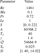
For our study we have chosen parameter values that yield as realistic a flame behaviour as possible whilst keeping the computational time reasonable. To achieve this, we use the values shown in table 3. The most prominent compromise that had to be made is the low Reynolds number and the large Mach number compared to experimental values (Blanchard et al.
Reference Blanchard, Schuller, Sipp and Schmid2015), yielding a large velocity upstream of the combustion zone of
 $35~\text{m}~\text{s}^{-1}$
and a small outer radius of the inlet at 0.64 mm. With our choice of chemical parameters, we reach a flame speed of
 $S_{d}=2.9~\text{m}~\text{s}^{-1}$
and a flame width of 0.007 mm, which amounts to approximately 1 % of the inlet-tube outer radius. Despite a discrepancy between parameters and values typically observed in real configurations, Blanchard et al. (Reference Blanchard, Schuller, Sipp and Schmid2015) showed that – for parameter values similar to ours – transfer functions could be obtained that match experimental results with acceptable accuracy. Although this agreement is not quantitatively accurate for all considered frequencies, the discrepancies are suggested to be due to the simple one-step, one-species chemical model used. A more sophisticated model with multiple species and reaction products is expected to produce more accurate results. An investigation into this issue, however, goes beyond the scope of this paper. Instead, we conclude from this verification that our model is consistent with the flame dynamics of earlier studies and captures the main features of its linear behaviour qualitatively well. The same former study also argued that, although the resulting flame speed is rather high for flames burnt in air, it constitutes a far more reasonable value for oxy-flames. The swirl number is kept in a low to moderate regime, certainly before the onset of vortex breakdown. This choice has been made to isolate the effect of increased mean-flow swirl on the gain, without the vortex breakdown mechanism (and the associated bifurcation of the mean-flow velocity profile) in play. Simulations are carried out for swirling and non-swirling cases and for forcing frequencies of
 $\unicode[STIX]{x1D714}\in \{1,2,3,4,6,10\}$
. Instead of the frequency, a Strouhal number, defined as
 $$\begin{eqnarray}\mathit{St}={\displaystyle \frac{\unicode[STIX]{x1D714}(r_{out}-r_{in})}{2\unicode[STIX]{x03C0}S_{d}/U}},\end{eqnarray}$$
is used to present our results. This definition of the Strouhal number differs from the one traditionally used in non-reactive fluid problems (see e.g. Garnaud et al. Reference Garnaud, Lesshafft, Schmid and Huerre2013), but is instead defined to allow for direct comparison with combustion experiments (Schuller, Durox & Candel Reference Schuller, Durox and Candel2003; Blanchard et al. Reference Blanchard, Schuller, Sipp and Schmid2015).
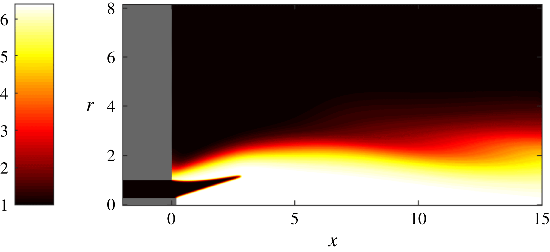
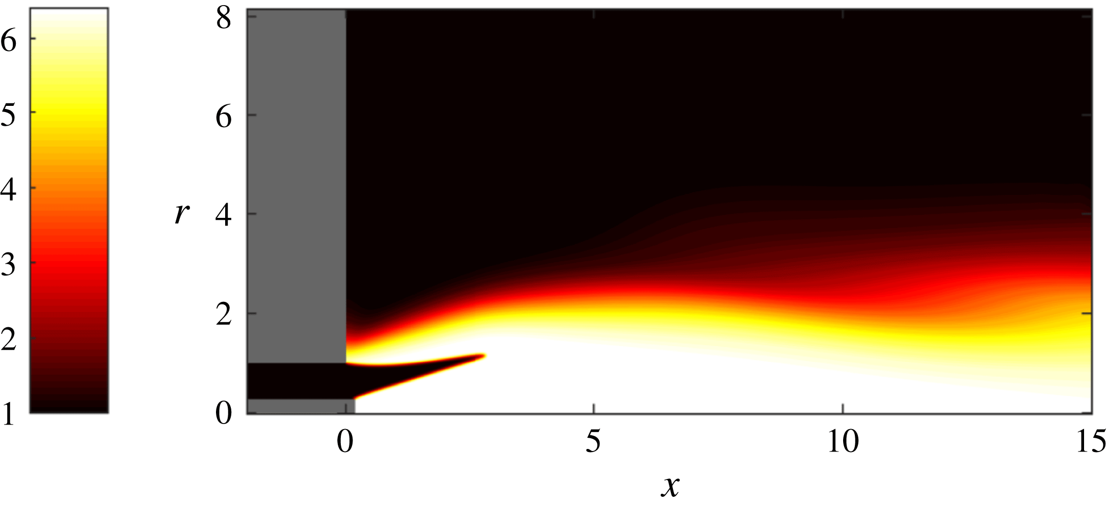
Isocontours of the non-dimensional temperature of a non-swirling base flow. The flame is attached at both the central rod and the outer inlet wall, producing its characteristic M-shape.
Parameter values used in our study.
3.1 No mean-flow swirl
We start by considering the optimal gains for an M-flame with no mean-flow swirl, which commences by finding a steady solution to the nonlinear axisymmetric equation. This base flow, visualised by the temperature field in figure 2, represents the equilibrium point about which the governing equations are linearised to find the Jacobian matrix
 $\unicode[STIX]{x1D63C}_{m}$
and its adjoint
 $\unicode[STIX]{x1D63C}_{m}^{\text{H}}$
. The optimal gains can then be computed using the above expressions; more specifically, the Lanczos SVD routine is utilised from the SLEPC library (Hernandez, Roman & Vidal Reference Hernandez, Roman and Vidal2005).
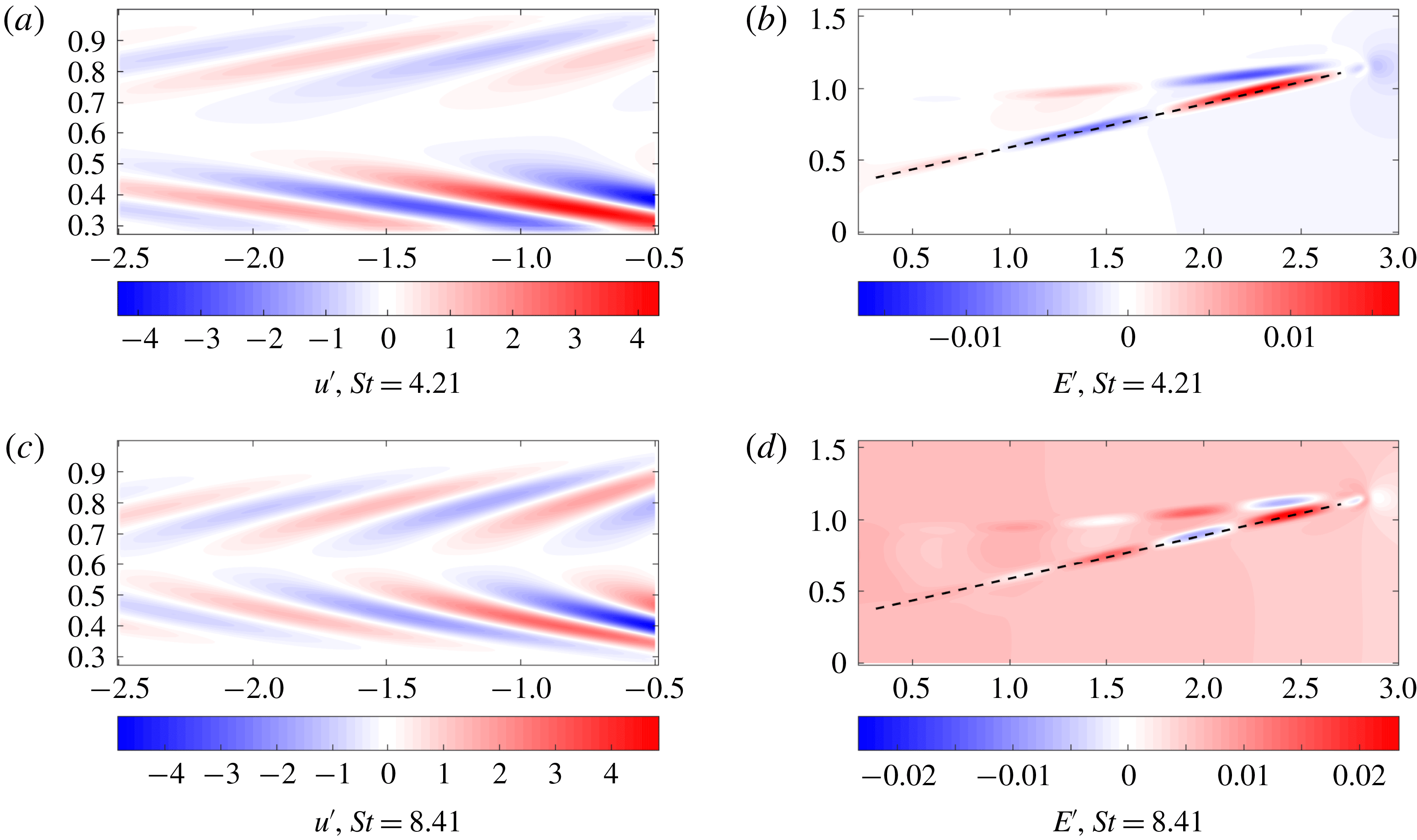
The optimal forcing and output are shown for
 $\mathit{St}=4.21,~8.41$
and
 $S=0,~m=0$
. The
 $u^{\prime }$
velocity component of the forcing is shown and the output is represented via the energy
 $E^{\prime }$
. The dotted line in the output panels indicates where data are taken from for the subsequent wave-speed calculation (see main text). For an animation of the above structures, see the supplementary movies 1–4 available at https://doi.org/10.1017/jfm.2018.793.

Figure 3 presents the optimal forcing and associated response at two forcing frequencies for
 $m=0$
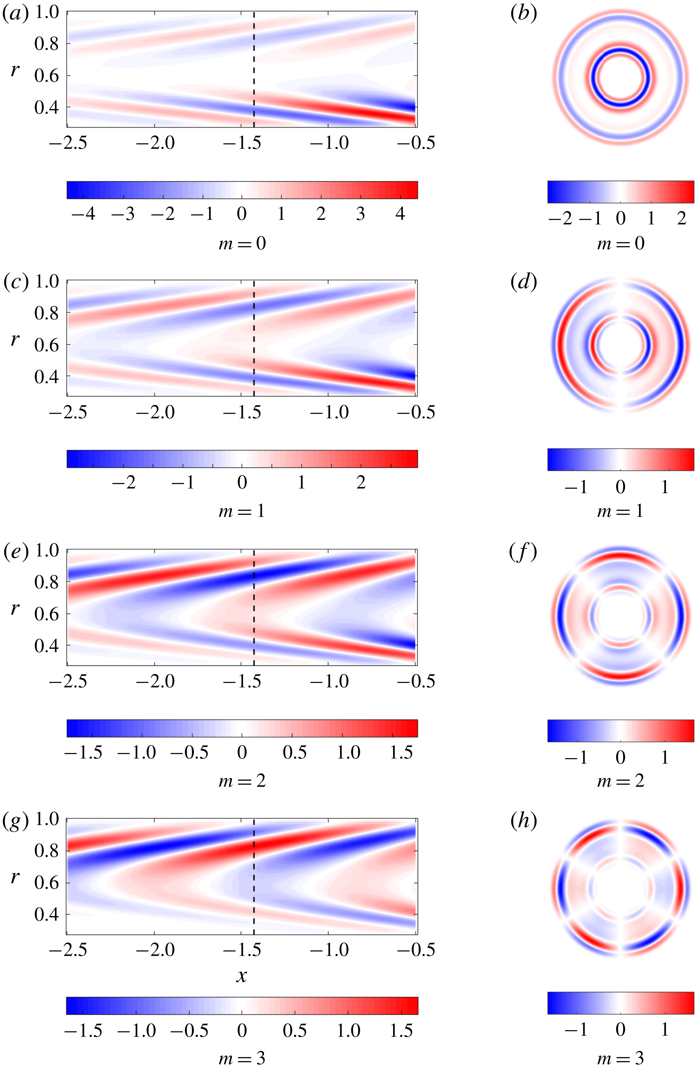
. The spatial structures for all state variables are similar and differ mainly in magnitude; hence, the shape of the optimal input and output is illustrated for only one representative variable. We note that the forcing consists of perturbations tilted against the mean flow, which generates as an output a wave confined to the flame front. This observation is typical of the Orr mechanism (Orr Reference Orr1907) in which perturbations aligned against the shear are advected by the mean flow and tilted by the mean shear (see Roy & Govindarajan (Reference Roy and Govindarajan2010) for more details). This energy amplification mechanism unravels as follows: First, the perturbations rotate, from their initial alignment against the shear, into the shear, extracting energy from the mean flow via Reynolds stresses. By overturning the perturbation structures, energy is scattered back to the mean flow via the same Reynolds-stress-based transfer process. The structures continue to be stretched by the mean shear, until dissipation dominates the final stage and diffuses the filaments. Ignoring viscous effects, the energy amplification due to the Orr mechanism can also be explained as a manifestation of Kelvin’s theorem: the circulation about a contour enclosing the initial structure (tilted against the shear) is conserved as the contour is advected by the mean flow. As the contour shortens due to advection, the velocity along it has to increase to preserve circulation. Beyond this point of maximum velocity, the contour again stretches in the shear field, and the associated velocity diminishes accordingly. Overall, we observe a transient amplification of velocity (energy), followed by ultimate decay. This process – combined with the typical flame mechanism of turning velocity perturbations into heat release at the flame front – underlies the mechanism that yields the optimal gain. For other azimuthal wavenumbers, the addition of azimuthal velocity in the optimal forcing causes a blending of the Orr mechanism with a lift-up mechanism, which utilises azimuthal shear to further contribute to the optimal gain. This blending can be seen in figure 4 where the slanted forcing (linked to the Orr mechanism) becomes less pronounced for higher azimuthal wavenumbers.
Increasing the forcing frequency decreases the wavelength of the forcing and of the output, and centres the forcing towards the middle of the annulus. This is exactly what was seen by Blanchard (Reference Blanchard2015), who used a non-swirling version of the numerical code to calculate the optimal gains for
 $m=0$
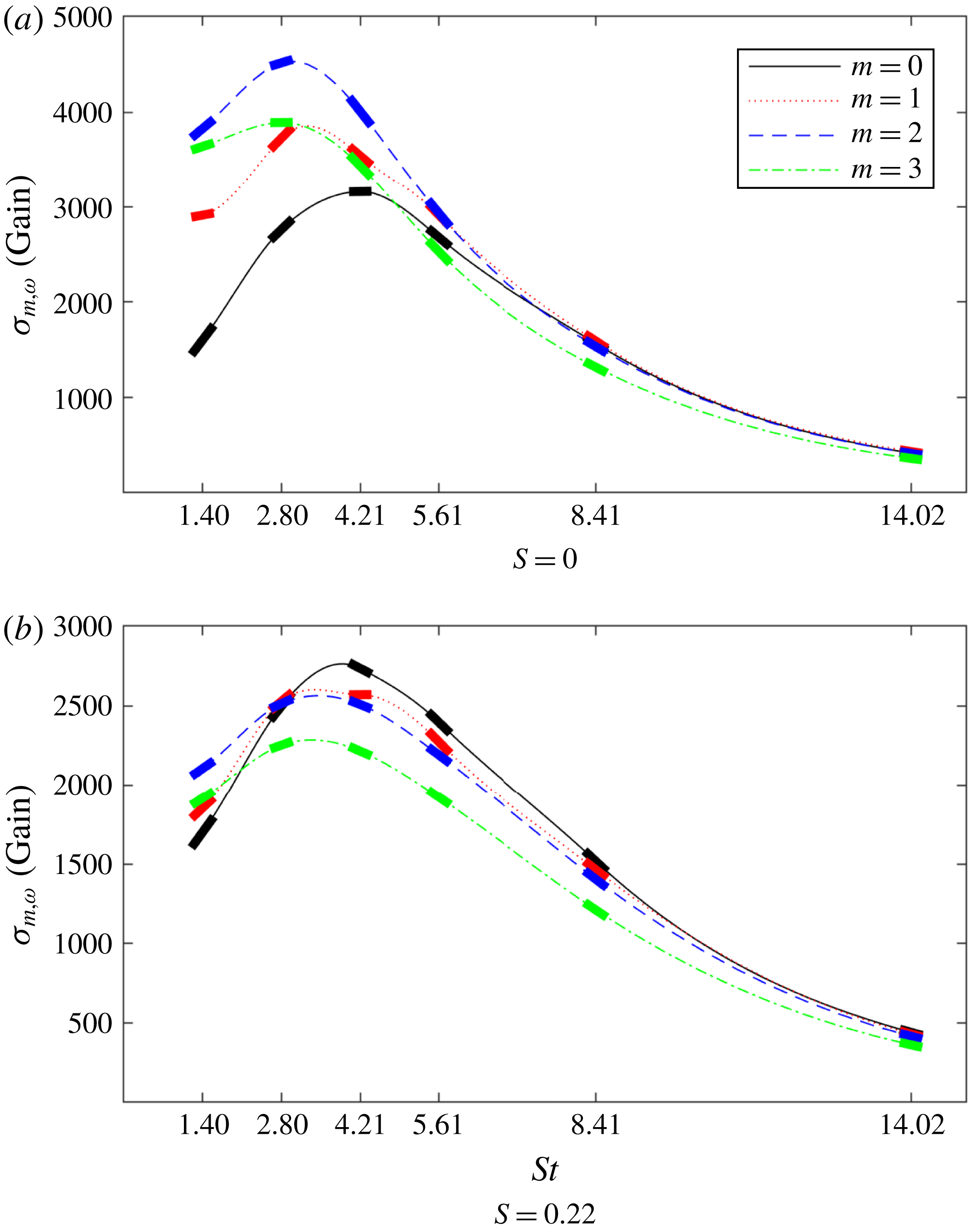
. We can also use his case to verify the growth-frequency curve shown in figure 5(a) for
 $m=0$
.
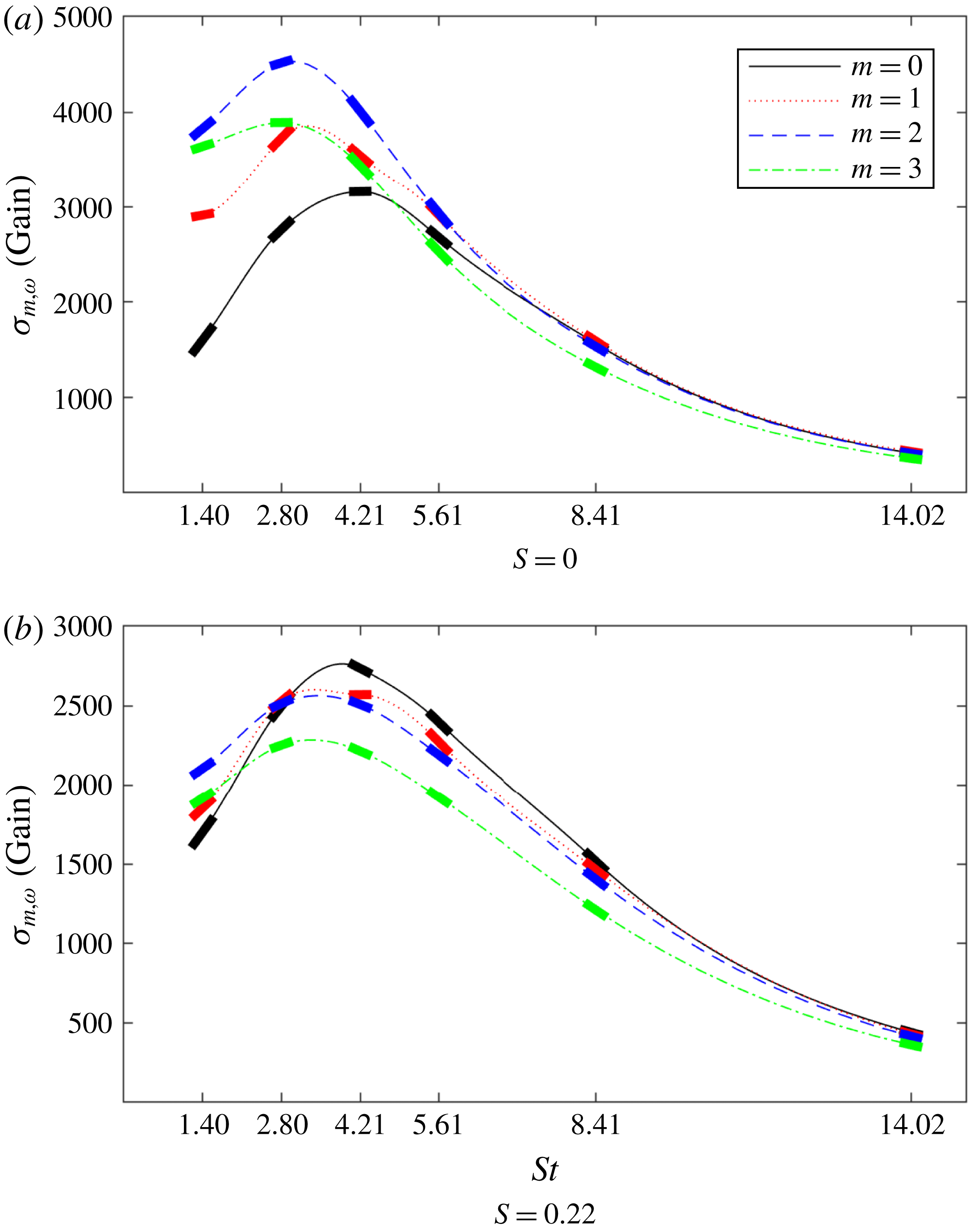
Figure 5(a) shows that increasing the azimuthal wavenumber
 $m$
has a positive effect on the peak gain up to the second mode. At first glance, this may seem odd since
 $m=1$
modes are commonly the most easily excitable owing to the fact that only they can support a non-zero radial velocity at the centreline (see Garnaud et al.
Reference Garnaud, Lesshafft, Schmid and Huerre2013, for example). However, for an M-flame configuration, the flame front is confined away from the centreline, resulting in a low radial mean-shear region near the centreline and hence no advantage for the
 $m=1$
mode to extract energy from the mean flow. It can be hypothesised that a V-flame would show similar behaviour to an M-flame due to the flame front location being similar. In the case of other flame shapes, such as, for example, the conical flame whose flame front crosses the centreline, the
 $m=1$
mode should be more prominent, as the optimal forcing mechanism now has the opportunity to properly exploit this mode’s unique property.
Besides observing the spatial structure of the forcing and output, it is equally important to determine the flow variables that contribute substantially to the optimal gain; this type of analysis is performed by splitting the norm into its constituent parts. We find that the forcing consists nearly exclusively of velocity perturbations, with negligible amounts of fuel mass fraction, temperature and density fluctuations. In contrast, the optimal output contains
 ${\approx}42\,\%$
of each temperature and fuel mass fraction perturbations, with density fluctuations accounting for the remainder. It is not surprising that mass fraction and temperature fluctuations contribute nearly equal amounts to the optimal gain, as the two are physically linked and our selected norm has been designed to reflect this fact (Blanchard Reference Blanchard2015). The observed distribution of state variables in the optimal output structures suggests that pressure fluctuations (via unsteady heat release) are the primary output quantity. This is commonplace and typical of thermoacoustic mechanisms in which velocity perturbations cause unsteady heat release, which subsequently yields acoustic pressure fluctuations. While this mechanism has often been advanced as the primary thermoacoustic process, our analysis has not biased towards this scenario, but rather included all flow variables and their combinations as ingredients for an optimal amplification mechanism. In this effort, it is found that, although longitudinal velocity perturbations are pivotal in producing optimal gains for
 $m=0$
, azimuthal and radial perturbations become progressively important for higher wavenumbers.
The longitudinal velocity component of the optimal forcing is shown for
 $\mathit{St}=4.21$
and
 $S=0.22$
for all wavenumbers. The dotted line shows where the plot is revolved around the axis to produce its corresponding polar plot. This clearly shows the azimuthal structures for the optimal forcing.

Optimal frequency response gains versus forcing frequency for two values of swirl. The thick solid line segments for each forcing frequency indicate the computed gradients from the parametric sensitivity analysis.
Indeed, for
 $m=3$
the contribution of azimuthal velocity components outranks the longitudinal components in the optimal forcing structure. Clearly, this finding would have been overlooked without an unbiased computational approach. Here, we shall recall that all results depend on the chosen norm. While we have found that, for our choice of norm, the optimal response is related to thermoacoustics, special care must be taken when interpreting results in the context of thermoacoustic instabilities. Thermoacoustic instability mechanisms depend not only on the amplification of certain variables but also on the phase relationship between pressure and heat release fluctuations. As our norm does not directly contain this information, the gains and output shapes shown in this study do not necessarily link to a thermoacoustic instability.
The dominance of structures with
 $m=2$
can now be explained. As noted in the previous paragraph, the forcing consists mainly of velocity perturbations. For the axisymmetric case (
 $m=0$
), these velocity perturbations are entirely concentrated in the longitudinal and radial directions, but for
 $m>0$
we also obtain azimuthal contributions. The axisymmetric structures develop in the absence of an azimuthal pressure gradient and azimuthal mean-velocity gradients; this same situation also prevents
 $w^{\prime }$
perturbations from reaching the flame front and deforming it. For
 $m>0$
we break axisymmetry, and non-axisymmetric perturbations are sufficiently sustained to induce hydrodynamic disturbances at the flame front. Moreover, for a non-zero azimuthal wavenumber
 $m$
, we obtain an
 $O(m)$
azimuthal advection and an
 $O(m^{2})$
azimuthal diffusion; hence, we expect a tradeoff between an increased azimuthal velocity due to advection and diminished velocities due to viscous diffusion. Clearly, for
 $m=2$
this tradeoff is in favour of intensifying the frequency response gain. Starting with
 $m=3$
, the balance apparently tips in favour of diffusive effects, and we expect to see a further decrease in peak gain for higher azimuthal wavenumbers as diffusion becomes even more dominant.
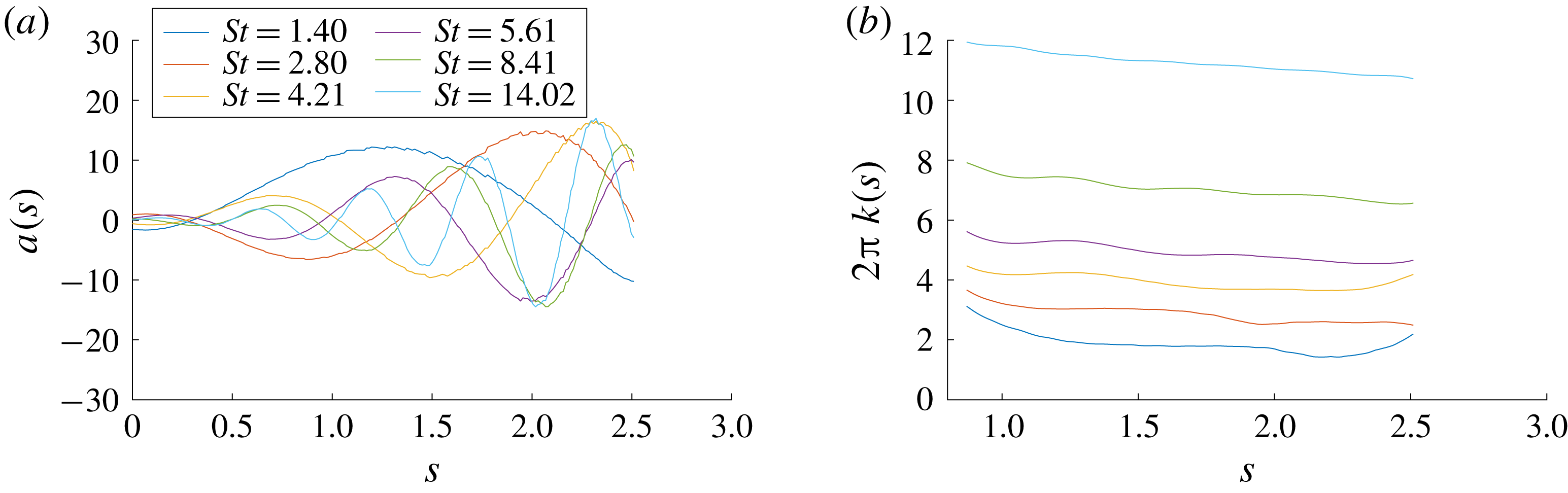
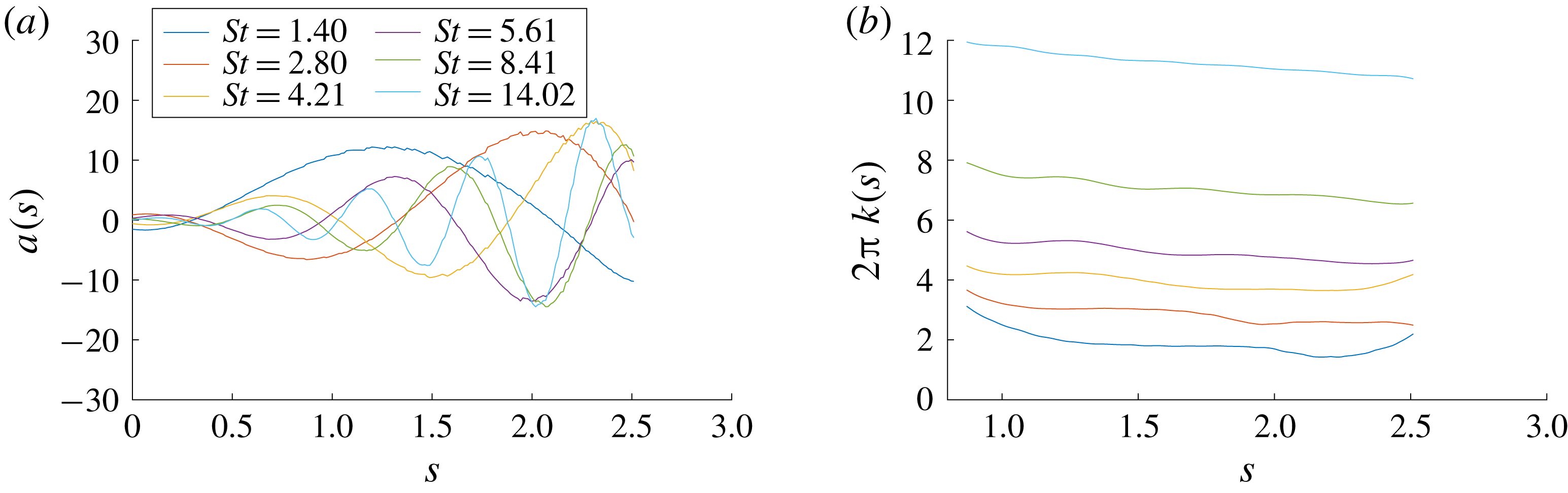
We can see from figure 3(b,d) that the optimal output consists of waves that advect down the flame front. The amplitudes of these waves are shown in figure 6(a). Using these series, as well as the corresponding series for the other frequencies, we can calculate the wavenumber for each forcing frequency using a Hilbert transform approach. To this end, we use the fact that a complex signal
 $z(s)$
along the linear (dashed) path can be generated from a real signal according to
 $$\begin{eqnarray}z(s)=a(s)+\text{i}{\mathcal{H}}\{a(s)\}=A(s)\exp (\text{i}\unicode[STIX]{x1D719}(s)),\quad {\mathcal{H}}\{a(s)\}=\unicode[STIX]{x2A0D}_{-\infty }^{\infty }{\displaystyle \frac{a(s-\unicode[STIX]{x1D709})}{\unicode[STIX]{x03C0}\unicode[STIX]{x1D709}}}\,\text{d}\unicode[STIX]{x1D709},\end{eqnarray}$$
with
 $s$
denoting the coordinate along the path and
 $a$
the amplitude of the signal. The imaginary part of
 $z$
consists of the Hilbert transform
 ${\mathcal{H}}$
of the same signal. From the phase
 $\unicode[STIX]{x1D719}(s)$
of this expression, we can then determine the local wavenumber
 $2\unicode[STIX]{x03C0}k(s)=\text{d}\unicode[STIX]{x1D719}(s)/\text{d}s$
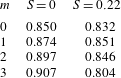
by simple differentiation. Computationally, this procedure can be improved upon by applying windowing techniques along the path, to circumvent excessive end effects from finite integration limits. Figure 6(b) shows the resulting local wavenumbers along the dashed paths in figure 3(b,d). All examined Strouhal numbers show a rather constant wavenumber along the flame front, with only minor shortening of the scales towards the flame tip for only the lowest Strouhal number. This finding supports the conclusion that the propagation of perturbations from the flame base towards the flame tip shows little dispersion and occurs at a non-dimensional phase speed of
 $c_{p}\approx 0.85$
. Animations of this associated perturbation dynamics based on linearised simulations corroborate this finding.
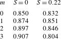
The phase speed has also been calculated for higher azimuthal wavenumbers and for increased mean-flow swirl, discussed more in § 3.2; the values are collected in table 4. We observe that the phase speed varies only slightly with
 $m$
, for either case of mean-flow swirl. This observation suggests that the propagation of perturbations towards the flame tip exhibits only a negligible amount of dispersion and that the azimuthal dependence of the perturbation is approximately preserved as it advances towards the flame tip.
The phase speed
 $c_{p}$
for all azimuthal wavenumbers, with and without mean-flow swirl.
3.2 Increased mean-flow swirl
By calculating a new base flow with a higher swirl number, we can next investigate the effect of increased mean-flow swirl on the optimal gains. We note that the new base flow has a similar M-flame temperature profile to that shown in figure 2. As a consequence, we will mostly see the effects due to the increase in swirl rather than the effects of a radically different base flow.
Figure 5(b), displaying the frequency response gains for various azimuthal wavenumbers and a non-zero swirl number, shows that there is a complete reordering in the peak gains, with
 $m=0$
giving the largest peak gain and all subsequent wavenumbers showing a decrease. The reordering is to be expected due to the
 $O(m^{2})$
diffusive effect now involving the mean-flow swirl. Owing to the presence of an azimuthal velocity in the base flow itself, the total energy exhibits increased diffusive effects, meaning that increasing
 $m$
results in decreased temperature perturbations at the flame front. If this were the only effect, we would still expect
 $m=0$
to be relatively similar to the non-swirling case; but instead we see a decrease in its gain, hinting that other physical mechanisms are at play. This issue will be further investigated in § 4.4. The composition of the optimal forcing and output are similar to the non-swirling case, indicating that the same processes for producing the optimal gain are at play. However, contrary to the non-swirling case, longitudinal velocity perturbations remain the dominant part of the forcing for all wavenumbers.
Spatial signal along the flame front, to be processed into a wave-speed value for
 $S=0$
,
 $m=0$
. The lines along which the data are obtained are shown as dashed lines in figure 3(b,d).
4 Parametric sensitivity analysis
4.1 Sensitivity with respect to the forcing frequency
In figure 5 we have shown the gradients of the gains with respect to swirl as bold line segments at each computed frequency, calculated using (2.20). By using not only the gain at each frequency but also its gradient, we are able to connect subsequent evaluation points using cubic polynomials, resulting in a smooth and continuous curve (cubic spline) for the frequency response gain. Access to the sensitivity with respect to frequency not only enables us to accurately cover a large range of frequencies by carrying out SVDs at only a few selected points, but also allows us to employ adaptive techniques in selecting the next evaluation point. For example, running a simulation for
 $\mathit{St}=2.80$
and
 $\mathit{St}=5.61$
for
 $m=0$
and
 $S=0$
, figure 5(a) shows nearly the same gain for each case; without further gradient information, this might suggest a flat region in the gain curve. However, by efficiently calculating the frequency sensitivity for both these points, a sign change is observed, suggesting that the gain curve attains a maximum between these selected frequencies. This potential maximum can be estimated by fitting a cubic spline between these two points and can be evaluated by computing an SVD at this estimated point. In the above case, the maximum can be confirmed, as can be seen in figure 5(a) with a maximum at
 $St=4.21$
.
4.2 Sensitivity with respect to the Reynolds number
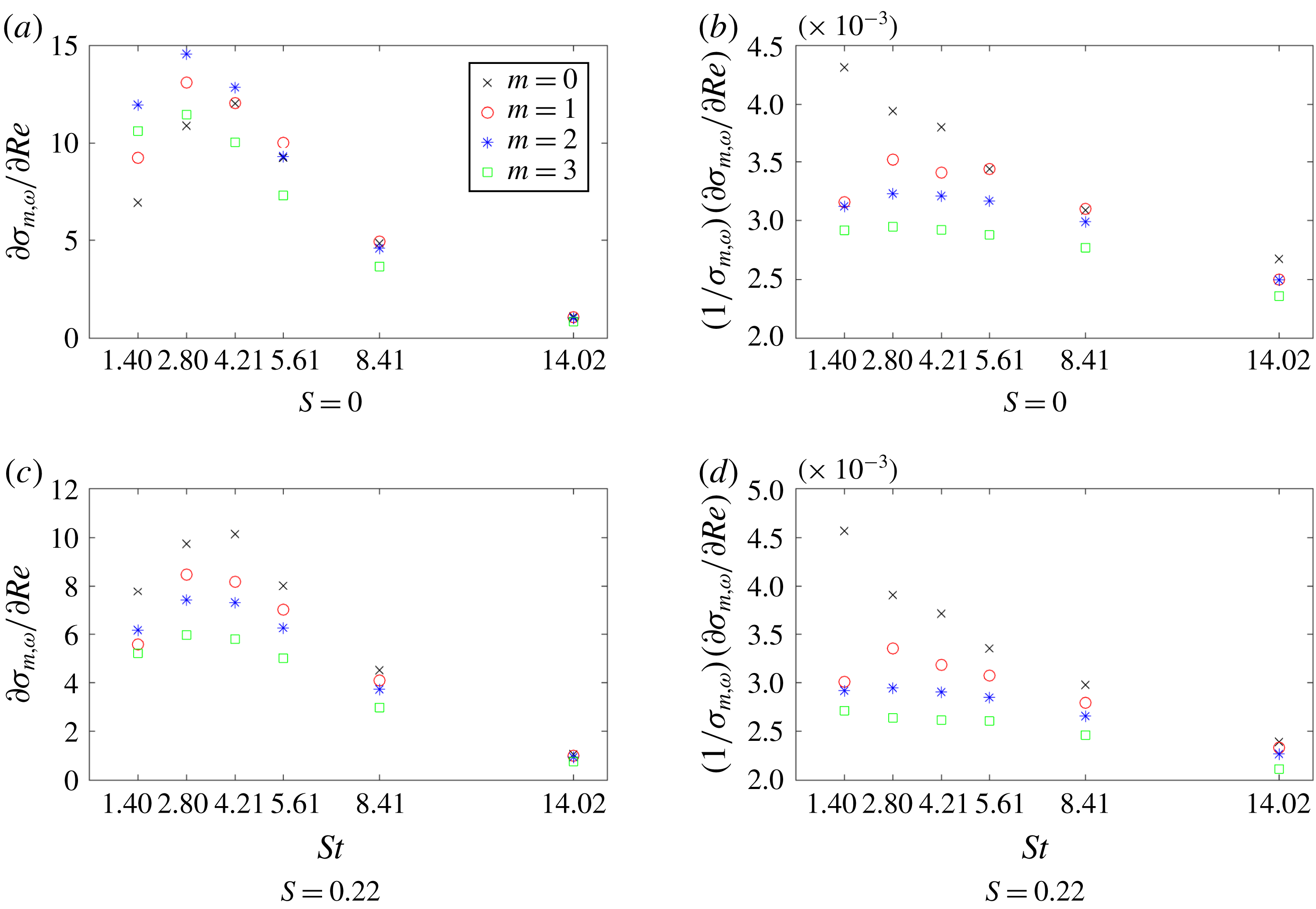
After calculating the sensitivity with respect to the forcing frequency for a better representation of the gain curve, we now proceed to determine the sensitivities with respect to the governing parameters of the problem. First, we compute the sensitivity with respect to the Reynolds number using (2.21). In our analysis, we make the additional assumption that a small change in Reynolds number does not change the base flow appreciably; in other words, only the influence of Reynolds number changes on the perturbations is considered. This constrains the variation in Reynolds number to its effect via the equations and neglects effects due to changes in the norm. As a consequence, we compute the derivatives (2.22) by keeping the base flow constant.
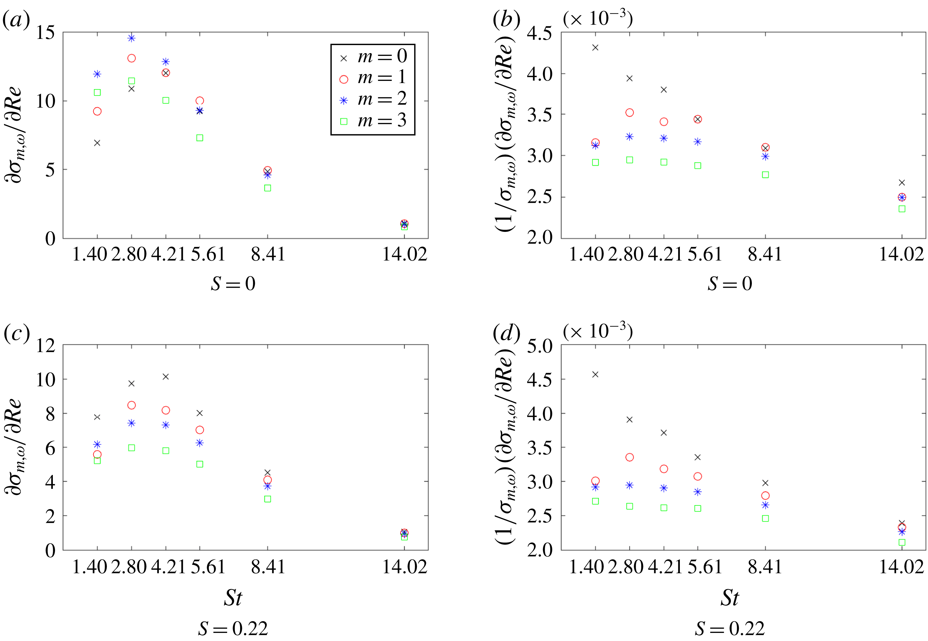
Figure 7 clearly shows that increasing the Reynolds number amplifies the peak gain across all wavenumbers. This is easily explained by the fact that Reynolds number changes occur as a viscous effect for both the velocity and the temperature, but since temperature is more abundant in the optimal response, it is the decreased temperature dissipation for an increased Reynolds number that is responsible for the majority of the contribution to the sensitivity. We can also see that Reynolds-number changes enlarge the gain in proportion to its original value for both the swirling and non-swirling case, i.e. a higher gain shows more significant increases. This will favour gain distributions with sharper peaks, concentrating the optimal frequencies to a more narrow region.
Sensitivity of the optimal gain with respect to the Reynolds number for
 $S=0$
and
 $S=0.22$
.
4.3 Sensitivity with respect to the Mach number
We next consider the sensitivity with respect to the Mach number. Again, we assume a constant base flow, but now consider the effect of changes in norm due to the explicit dependence of the Chu norm on the Mach number. In contrast to the sensitivity with respect to the Reynolds number, where only one physical mechanism has been involved, changes in the Mach number instigate corresponding variations via multiple processes.
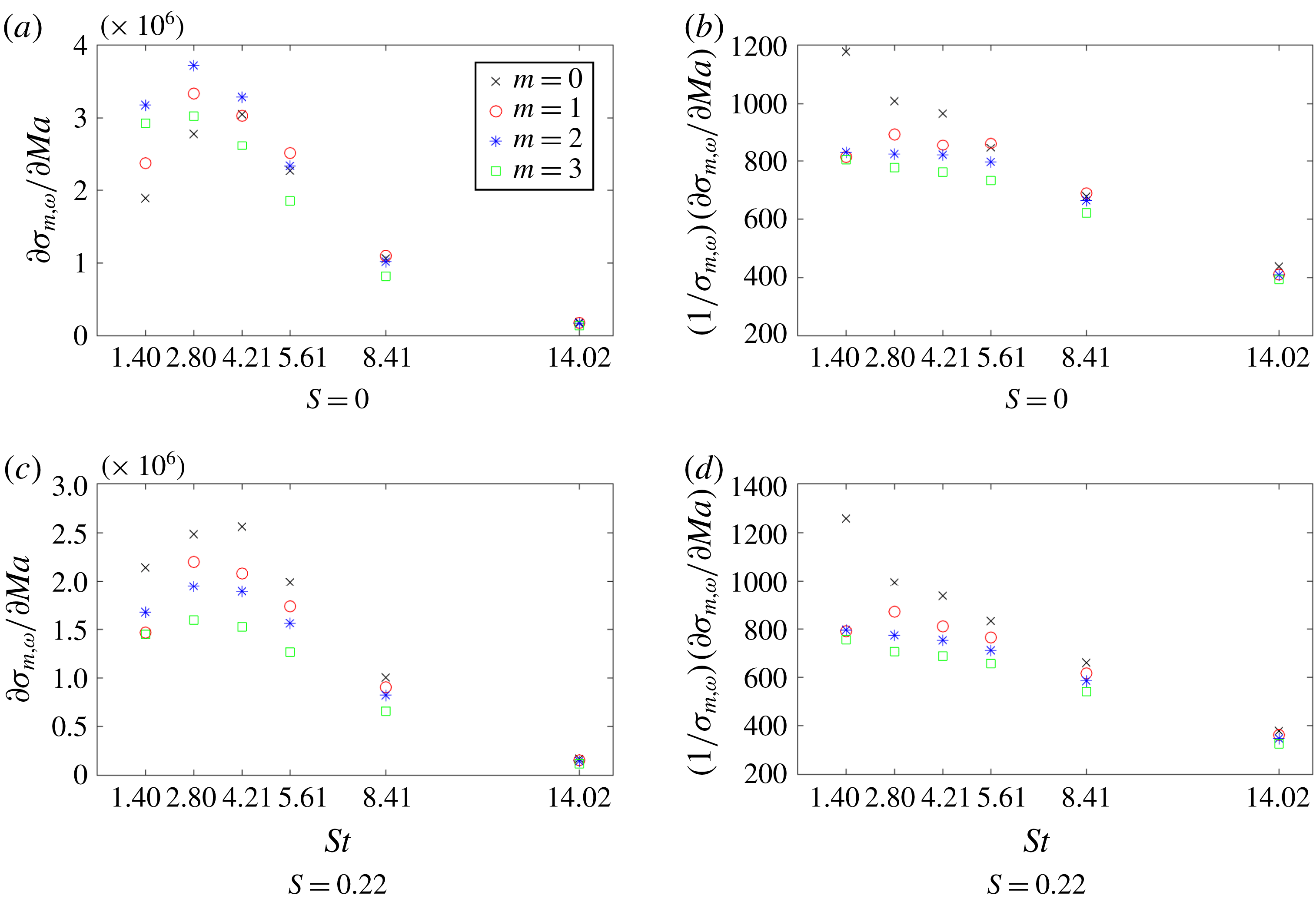
Sensitivity of optimal gain with respect to the Mach number for
 $S=0$
and
 $S=0.22$
.
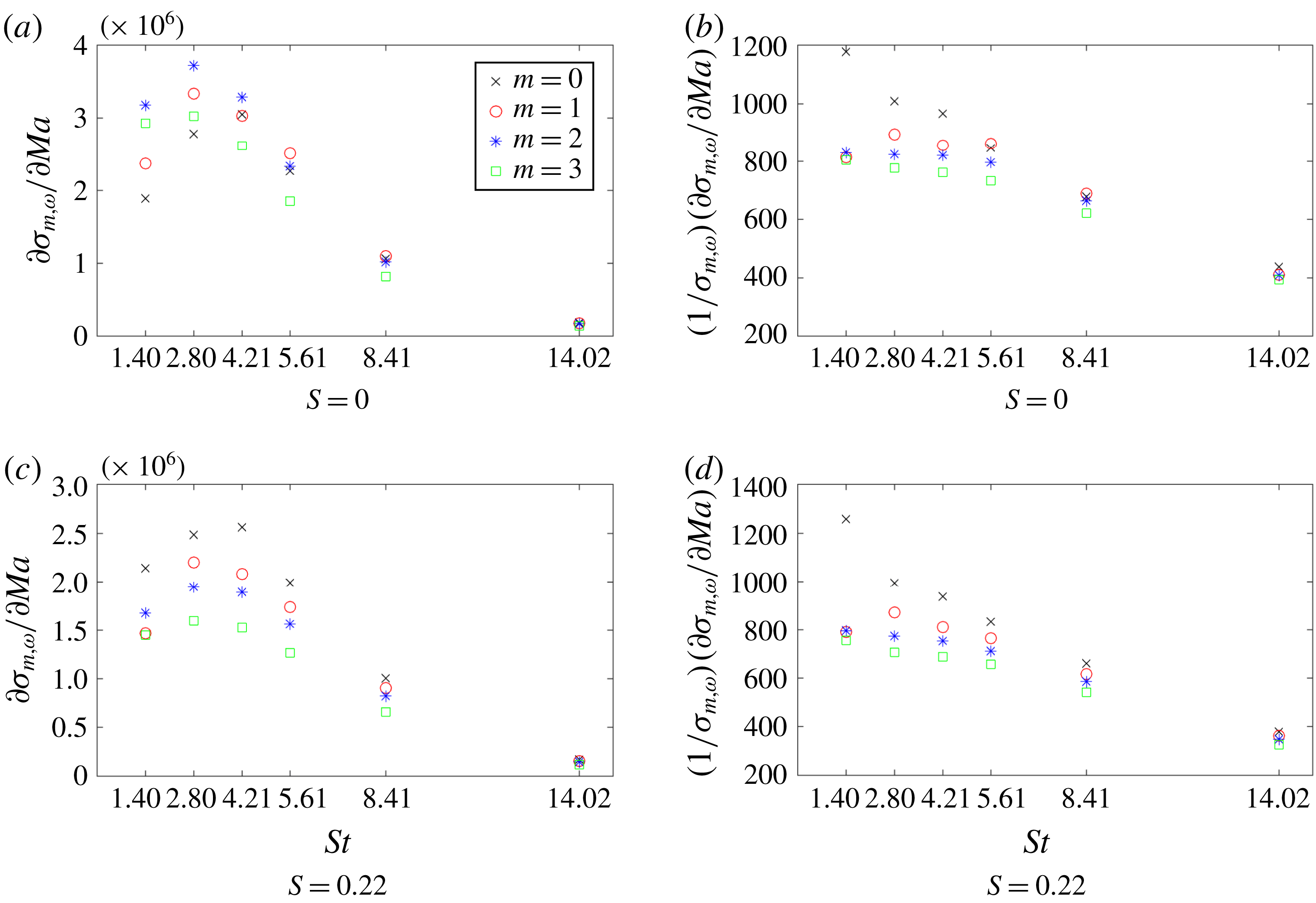
We see from figure 8 that, similar to the previous case, positive Mach-number changes are acting as amplifiers of the peak gains. This amplification is many orders of magnitude larger than in the Reynolds-number case, however, showing that the frequency response output is highly sensitive to changes in the Mach number. Even though we now consider effects due to the change in the norm, the relative contribution of this effect to the overall sensitivity is found to be rather negligible. In other optimal forcing studies, such as the work of Fosas de Pando & Schmid (Reference Fosas de Pando and Schmid2017), the Mach number is shown to be responsible for mode shifting rather than simple amplification. This mode shifting is reflected in a sign change in the sensitivity at a maximum or minimum of the peak gain and is caused by a modification of the acoustic travel time, thus causing the optimal forcing to move out of phase with the optimal input. The reason we do not see this mode-switching behaviour in our case is due to the fact that the mechanism responsible for the optimal gain is based on hydrodynamic rather than acoustic disturbances.
Reynolds-number and Mach-number sensitivities (see figures 7 and 8) show similar behaviour, except for the magnitude, as both the Reynolds and Mach numbers appear in the coefficient of the temperature diffusion in the energy equation (2.3); therefore, they both produce similar contributions to the sensitivity – except that their effects are
 $O(Re^{-1})\approx 7\times 10^{-4}$
and
 $O(Ma^{-2})\approx 1\times 10^{2}$
, respectively, giving rise to a difference of six orders in magnitude.
4.4 Sensitivity with respect to the swirl number
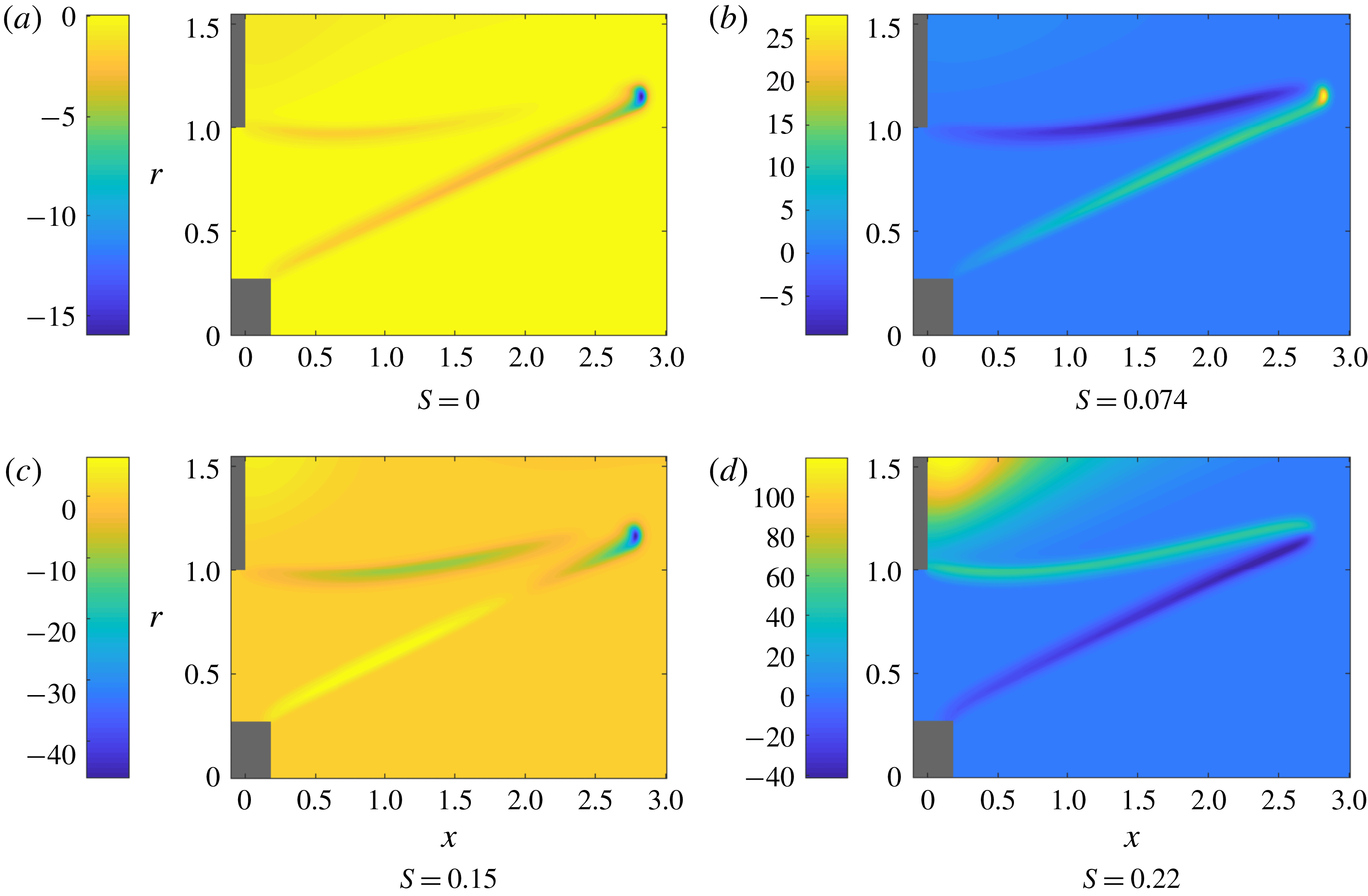
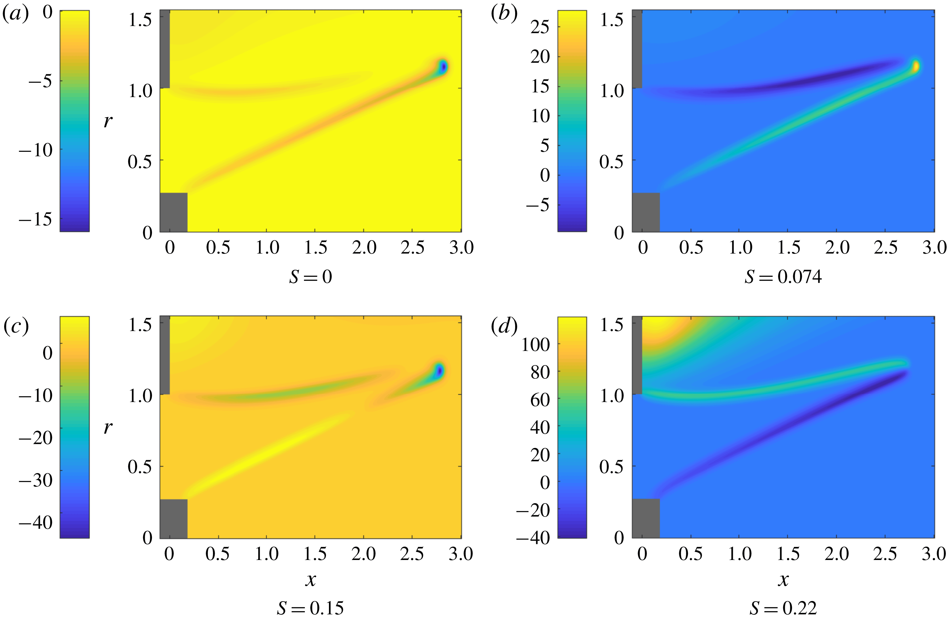
Similarly to the cases above, we can calculate the sensitivity with respect to the swirl number using (2.21). However, unlike the previous examples, changes in swirl number manifest themselves not via terms in the linearised equations but entirely via the base flow; this means that we must consider base-flow changes when computing the derivatives (2.2). New base flows with slightly higher swirl numbers have been determined for this purpose. The temperature component of the base-flow derivatives for various swirl numbers is displayed in figure 10. Besides a rather uniform influence along the flame front, it shows a concentration of sensitivity amplitudes at the flame tip; sensitivities with respect to other variables display similar qualitative behaviour.
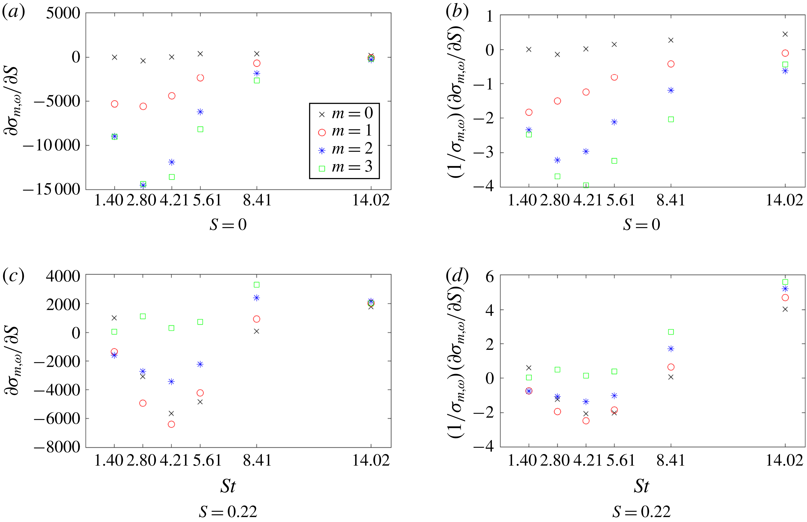
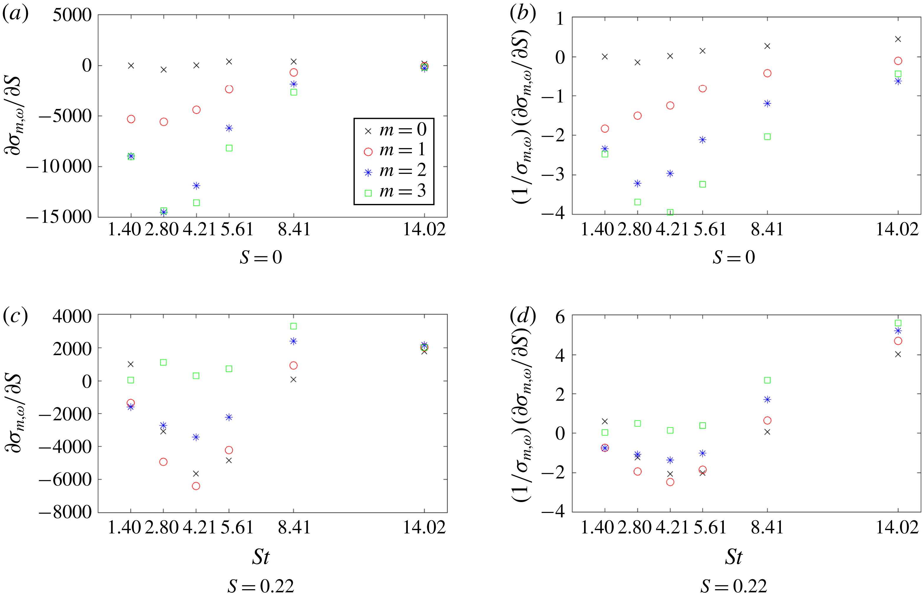
Sensitivity of the optimal gain with respect to the swirl number for
 $S=0$
and
 $S=0.22$
.
Temperature component of the derivative of the base flow with respect to the swirl number, shown for four different swirl numbers.
Frequency response gain versus swirl number for all considered wavenumbers and
 $\mathit{St}=4.21$
. The thick solid line segments represent the gradient at that point. The plot is interpolated between consecutive calculated gains using cubic Hermite splines to match both the values and gradients.
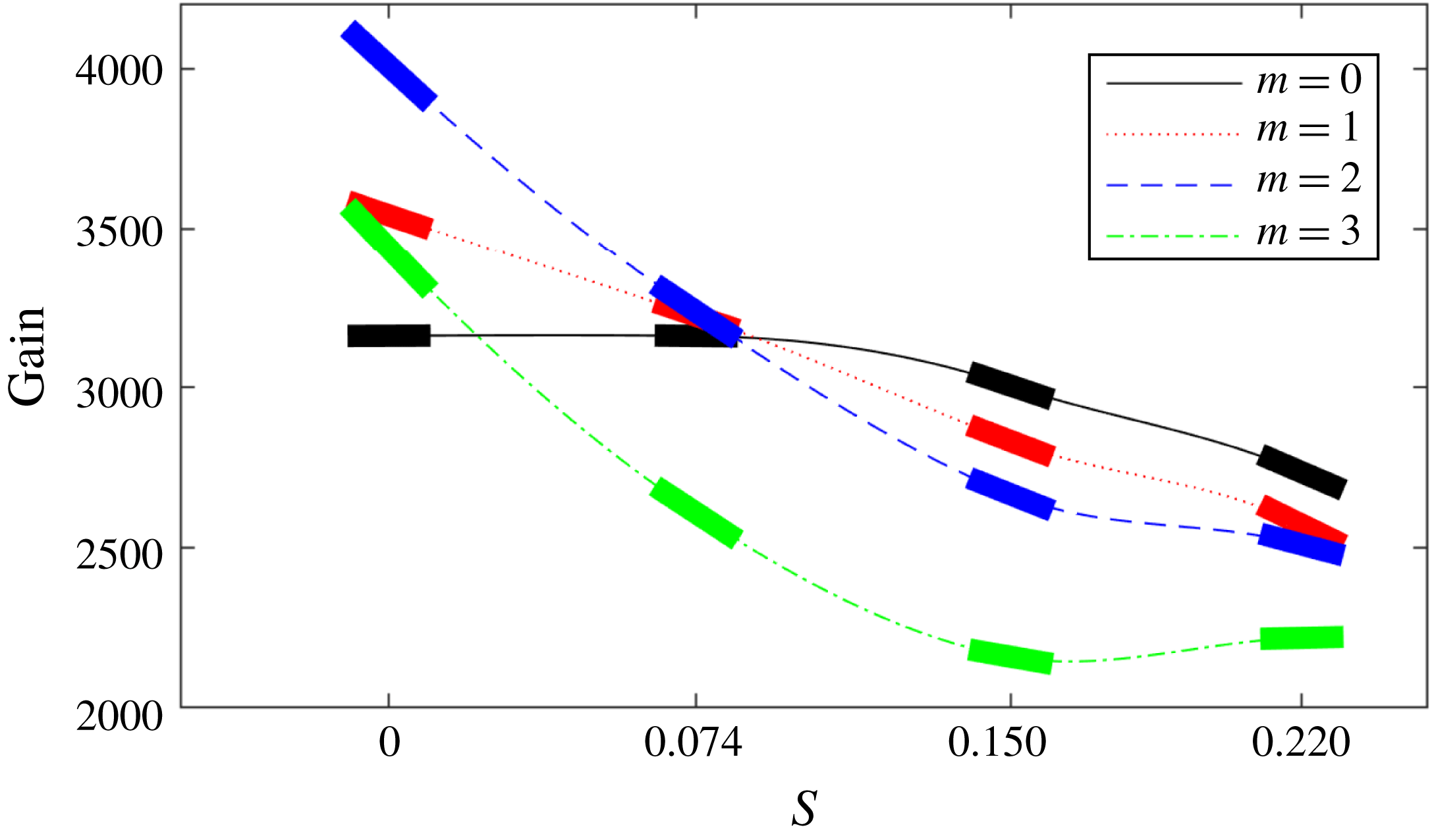
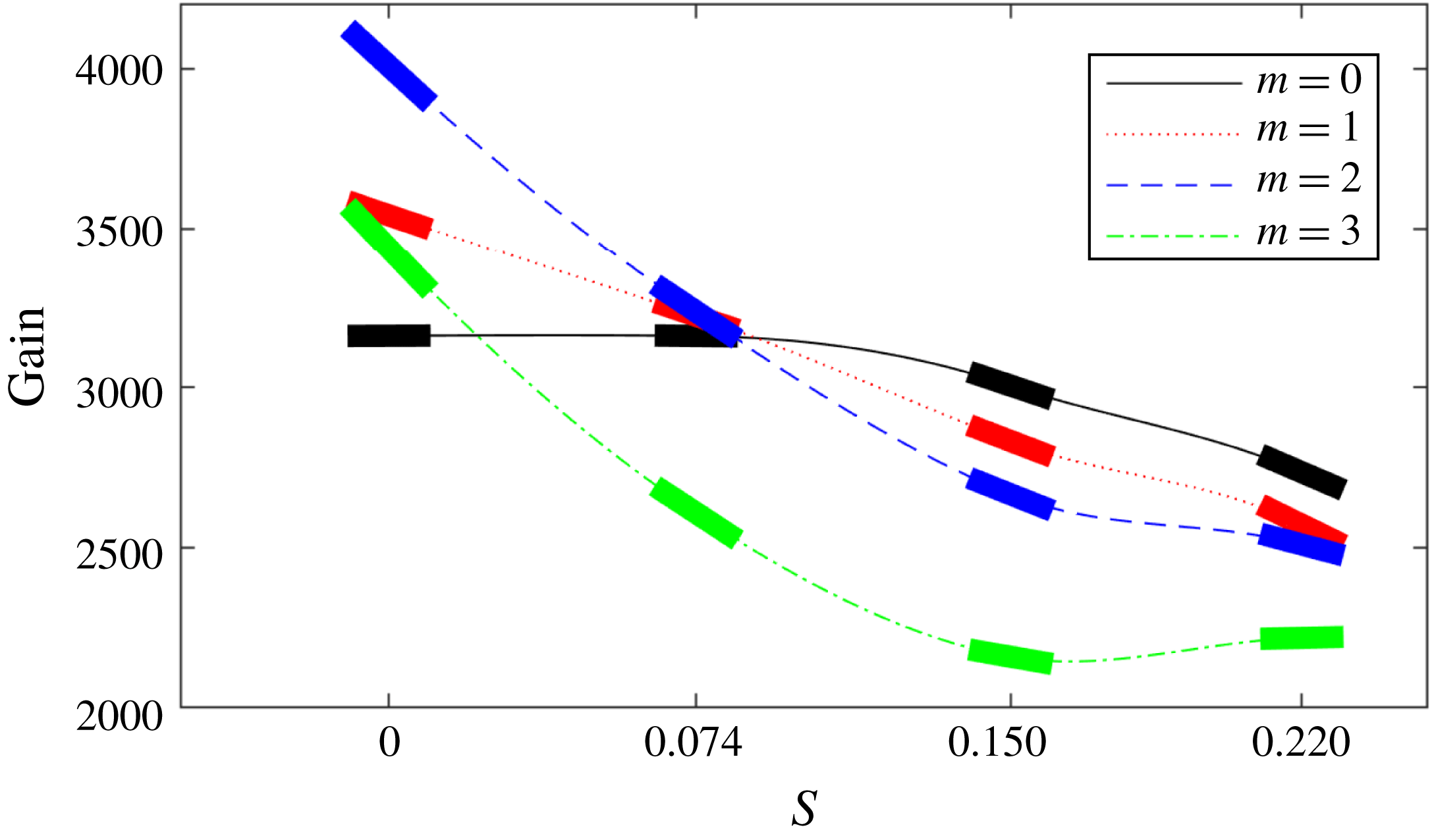
Figure 9(a), attained for zero swirl, reconfirms the behaviour shown previously: axisymmetric (
 $m=0$
) modes are characterised by smaller sensitivities when compared to non-axisymmetric, higher modes. The case of non-zero mean-flow swirl, shown in figure 9(c), reveals a more interesting behaviour. First, all modes are now displaying an increase in gain for high Strouhal numbers. In addition, for the Strouhal numbers where the peak gains have been found, we observe a decrease for all modes, except the
 $m=3$
mode, which exhibits a slight increase. Nonetheless, these effects are small compared to the sensitivities we saw in the non-swirling case. The axisymmetric (
 $m=0$
) and shift (
 $m=1$
) modes are showing the greatest sensitivity. This can be directly related to our earlier observations where we argued that the
 $O(m^{2})$
diffusive effects involving the mean-flow swirl in the base flow are responsible for the observed decrease in the peak gains. However, this argument cannot explain the decrease in the axisymmetric (
 $m=0$
) mode.
We can note from figure 11 that for
 $\mathit{St}=4.21$
the gain for all wavenumbers behaves linearly across the range
 $0\leqslant S\leqslant 0.09$
. As discussed in § 3.1, this tendency can be attributed to azimuthal diffusion terms. In fact, the constant nature of the
 $m=0$
mode throughout this range provides further evidence, as this mode is not affected by azimuthal diffusion. Beyond this range, the behaviour for all modes begins to change in a nonlinear manner. This latter behaviour must then be ascribed to nonlinear changes in the base flow as the
 $m=0$
mode starts to be damped. Figure 10 shows that, as we add swirl, there are drastic and fundamental variations in the base flow at the flame front; these variations and the corresponding gradients become larger as the swirl is increased further. For low swirl, the bulk of the base-flow sensitivity arises at the flame tip, but as swirl increases we notice a shift towards locations of high sensitivity along the entire flame front, leading to substantial base-flow changes for small increases in swirl. It is these more complicated changes in the base flow, observed at higher swirl numbers, that give rise to the above-mentioned nonlinear behaviour, such as the damping of the axisymmetric (
 $m=0$
) mode.
4.5 Validation of swirl sensitivities
The validation of gain sensitivities with respect to the Reynolds number has been reported earlier (Skene & Schmid Reference Skene and Schmid2017). A sensitivity analysis with respect to the Mach number will follow the same conceptual steps, since both parameters enter directly through the linearised governing equations. Gradients with respect to the swirl number proceed along a different path, involving changes in the base flow that bring about changes in the frequency response. For this reason, we test our adjoint-based sensitivities by predicting the frequency response gain at a swirl number of
 $S=0.074$
using the expansion
 $$\begin{eqnarray}\unicode[STIX]{x1D70E}_{pred.}\big|_{S=0.074}\approx \unicode[STIX]{x1D70E}\big|_{S=0}+0.074{\displaystyle \frac{\unicode[STIX]{x2202}\unicode[STIX]{x1D70E}}{\unicode[STIX]{x2202}S}}\bigg|_{S=0}.\end{eqnarray}$$
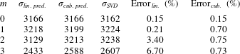
Table 5 summarises the results of our test. We see that the adjoint-based sensitivities are able to acceptably predict the decrease in gain experienced by increasing the swirl for all azimuthal wavenumbers. The relative prediction error is more accurate for lower wavenumbers (with values far less than 1 %); for higher azimuthal wavenumbers, the relative error rises to a few per cent. For predictions of the frequency response gain at higher swirl numbers, we have to recall the nonlinear behaviour discussed in the previous section. Consequently, a linear extrapolation, based on (4.1), is expected to deteriorate in accuracy in this parameter regime. In this case, we replace the extrapolation approach by an interpolation approach: more specifically, we harness the gain values at specific Strouhal numbers together with their adjoint-based gradients with respect to the swirl number to construct a cubic Hermite spline between these two evaluation points. Evaluating the spline at
 $S=0.15$
produces an estimate for the gain at this Strouhal number. In this manner we are able to better capture the nonlinear gain–swirl relation for higher swirl numbers. Table 5 verifies that the above cubic Hermite interpolation technique produces predictions with relative errors less than 1 %, even for the higher azimuthal wavenumbers.
Predicted gains
 $\unicode[STIX]{x1D70E}_{lin.\,pred.}$
and
 $\unicode[STIX]{x1D70E}_{cub.\,pred.}$
, actual gains
 $\unicode[STIX]{x1D70E}_{SVD}$
and relative errors for
 $S=0.074$
. The predictions are made using linear extrapolation or cubic Hermite interpolation. The corresponding errors are shown for both cases.

This above validation case also brings out an important point in our parametric sensitivity analysis: the inclusion of gradient effects stemming from changes in the chosen norm. If we examine the swirl sensitivity at
 $\mathit{St}=4.21$
for the axisymmetric case (
 $m=0$
), we find a value of
 $\unicode[STIX]{x2202}\unicode[STIX]{x1D70E}/\unicode[STIX]{x2202}S\approx 41$
, suggesting a very minor susceptibility to changes in swirl (see figure 9
a). This small value is obtained owing to a cancellation between an increase in gain of
 $1585$
directly from the equation and a decrease in gain of
 $1544$
due to associated changes in the norm. In addition, we can state that the bulk of the decrease in gain due to the norm stems from the norm of the output. This is not entirely surprising as the output is three orders of magnitude larger than the forcing. If we had not included the effect due to changes in the norm, we would have grossly overpredicted a change in gain due to variations in the swirl number. As an aside, this also stresses the importance and motivates the use of physically relevant norms to measure output quantities. In the above example, using the convenient, but unphysical,
 $2$
-norm would suggest sensitivities that would not be observed under realistic conditions.
5 Conclusions
A linear study of flame behaviour, based on the compressible Navier–Stokes equations with a simple, one-step irreversible chemical reaction, has been conducted to assess the response behaviour to harmonic forcing for an M-flame configuration. While FTFs are commonly applied to relate velocity perturbations to heat-release fluctuations, the approach taken in our study has been based on optimal frequency response gains given by the norm of the resolvent operator. This type of analysis not only determines the gain, but also identifies the input and output structure of the optimal amplification process and thus provides insight into preferred physical mechanisms. In our study, special emphasis has been put on the influence of base-flow swirl on the frequency response. We determined that for no base-flow swirl the
 $m=2$
azimuthal mode dominates due to the most favourable balance of azimuthal advection to viscous diffusion. We could further demonstrate that in the axisymmetric case (
 $m=0$
) the Orr mechanism is responsible for producing the largest gains, with velocity perturbations in the inlet being converted into mass fraction and hence temperature disturbances on the flame front. The addition of base-flow swirl reduces the output norm proportionally to
 $m$
and causes a reordering of the modes in terms of frequency response, to where the axisymmetric mode is most easily amplified. In the low-swirl regime this effect appears to be linear, causing the gain for the axisymmetric mode to stay constant. But as the swirl number increases, even to only moderate values, nonlinear changes in the base flow at the flame front cause nonlinear changes in the swirl–gain response, reducing the gain in the
 $m=0$
mode as well.
A second and equally important objective of our study was the demonstration of an adjoint-based sensitivity analysis for a highly parametrised fluid problem and the development of numerical techniques to extract a maximum of information over a maximum of parameter space with a minimum of computational effort. Our study achieves this by expanding upon previous work to include sensitivity effects stemming from direct parameter dependences in the chosen norm and to generalise the techniques to input and output quantities that do not spatially overlap. Sensitivities with respect to the forcing frequency and any other physical parameter of the system can be obtained from generic gradient information, contained in the adjoint variables. The efficient evaluation of frequency sensitivity has been shown to greatly aid in decreasing the number of required simulations and in detecting all pertinent maxima and minima in the frequency response curve. For sensitivities with respect to any governing parameter – in our specific case the Reynolds, Mach and swirl numbers – gradient information was shown to be useful in two distinct ways. First, as a way of extrapolating our results from a reference case to higher or lower values of that particular parameter for reasonable accuracy. Second, as a way of interpolating our results between two reference values of the gain. In either case, we gain valuable information about the response surface in parameter space at very reduced cost. This is particularly important for fluids problems (like ours) that are governed by many important parameters that would not otherwise allow an exhaustive parameter study. In addition, both techniques can be used for an adaptive exploration of parameter space, where subsequent simulations are chosen based on the sensitivity information found so far. By interpolating the gains between computed values, coarser arrays of simulations are needed to cover a larger range of parameters or frequencies.
Acknowledgements
We would like to thank the HPC service at Imperial College London for providing the computational resources used for this study. An EPSRC PhD Fellowship and support from the Marie Curie International Training Network ‘SSeMID: Stability and Sensitivity Methods for Industrial Design’ of the European Union are gratefully acknowledged. M. F. de Pando is thanked for stimulating and fruitful discussions.
Supplementary movies
Supplementary movies are available at https://doi.org/10.1017/jfm.2018.793.