1. Introduction and Background

To discuss the response of the Greenland ice sheet to global warming and its contribution to sea-level rise using a numeri-cal ice-sheet model, it is necessary to investigate several uncertainties related to the model itself. The uncertainties arise from imperfect modeling of physical processes such as basal sliding, ice stiffness, ablation and calving (Reference Ritz, Fabre and LetréguillyRitz and others, 1997). Moreover, numerical procedures such as model resolution affect the uncertainties (Reference Ritz, Fabre and LetréguillyRitz and others, 1997). Reference Hindmarsh and PayneHindmarsh and Payne (1996) and Reference Huybrechts and PayneHuybrechts and others (1996) have shown using an ideal isothermal ice-sheet model that the numerical procedure itself introduces a certain margin of error into simulation. This paper therefore discusses how simulation of the response of the ice sheet to warming is influenced by the numerical structure employed.

Ice-sheet models can be divided into two main groups based on the numerical methods used for mass-balance calculations (Reference Hindmarsh and PayneHindmarsh and Payne, 1996; Reference Huybrechts and PayneHuybrechts and others, 1996). Typically, the mass-balance equation in the flux form,

(1)

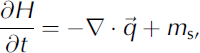
is rewritten in diffusion form as follows:

(2)

where H is the ice thickness, b is the bedrock elevation, is the ice-flux vector and m _s is the surface mass-balance term (accumulation minus ablation). The term D is a non-linear diffusion term that is calculated under the shallow-ice approximation as follows:

(3)

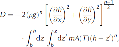
where ρ is the ice density, g is gravity acceleration, h is surface elevation, A is the temperature-dependent rate factor, and m is the enhancement factor. The ice flux is evaluated in terms of D as

(4)

In the horizontal discretization of Equation (1), the q term is typically evaluated on the mid x points. Thus, using the second-order central difference and the staggered grid system, the evolution of thickness at gridpoint (i,j) requires four terms: and D_{i , j + 1}/₂, as given by Equation (2). In one of the methods presented in Reference Hindmarsh and PayneHindmarsh and Payne (1996), D_{i+ 1} 2,j is evaluated directly using a staggered grid as follows:

(5)

where

(6)

(7)

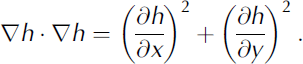
In another method, D_{i +1}/₂,j is evaluated by the average of two adjacent gridpoints, as given by

(8)

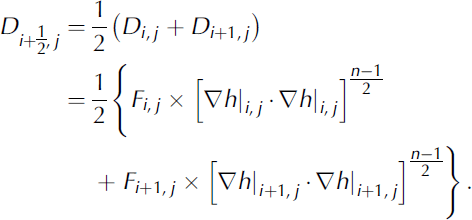
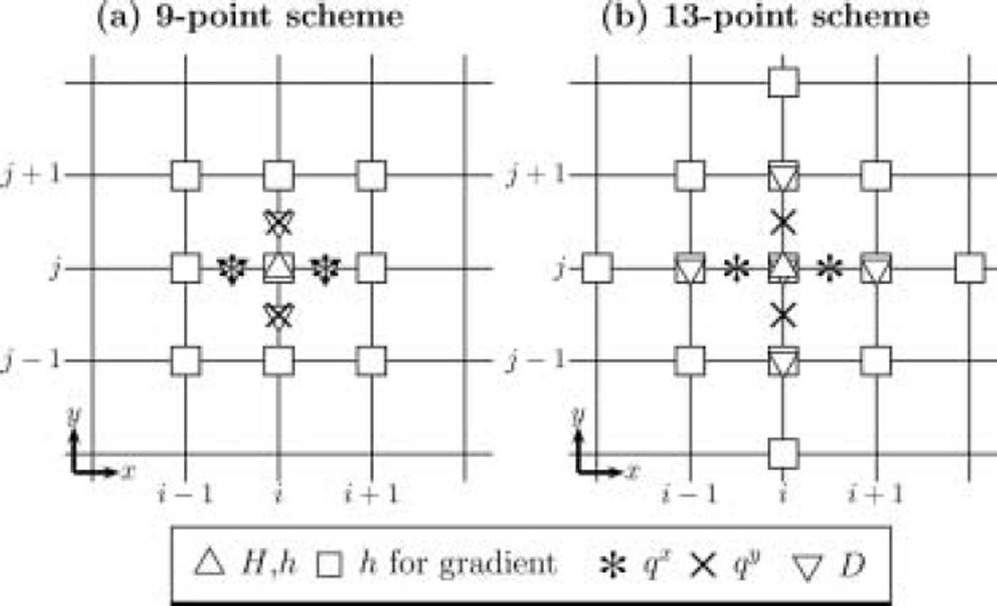
A similar treatment can also be used for D_{i , j} +1/2. Adopting the second-order central difference for computation of the surface gradient, the first method uses a total of 9 adjacent points to compute one gridpoint, whereas the second method uses 13 points. Thus, the two methods are referred to here as the 9-point scheme and the 13-point scheme, respectively. The two methods are illustrated in Figure 1. The 9-point scheme, deriving from the method of Reference MahaffyMahaffy (1976), is mass-conserving but has poor stability properties. In contrast, the 13-point scheme, derived originally from Reference HuybrechtsHuybrechts (1992), is stable for much larger time-steps (Reference Huybrechts and PayneHuybrechts and others, 1996), but opinions differ on its mass-conservation properties (Reference Hindmarsh and PayneHindmarsh and Payne (1996) maintain that it is mass-conserving, while Reference Huybrechts and PayneHuybrechts and others (1996) state that it is not). The present study compares the two schemes without discussing the relative performance. Reference Hindmarsh and PayneHindmarsh and Payne (1996) reported that for an isothermal ice-sheet model the 9-point scheme overestimates the steady-state thickness while the 13-point scheme gives an underestimate compared to the analytical (exact) solution.

Fig. 1.

Models for evaluation of D. Indices i and j are grid number of the model domain in the x and y axes, respectively. Symbols are gridpoints to evaluate each term. The term H is ice thickness, h is surface elevation, q_x and q^y are horizontal flux, and D is the nonlinear diffusion term (see text).

It is important to note that in both cases the error increases towards the margin. As ablation is generally active near the margin due to the higher temperatures that occur at lower elevation, the simulated response is directly affected by the error near the margin. This becomes a particularly important consideration in global warming experiments with elevation–ablation feedback, i.e. the lower the elevation the more melting occurs. Sensitivity experiments have been conducted by a number of authors for the Greenland ice sheet under spatially uniform background warming (Reference Letréguilly, Huybrechts and ReehLetréguilly and others, 1991; Reference Abe-OuchiAbe-Ouchi, 1993; Reference Fabre, Letréguilly, Ritz and MangeneyFabre and others, 1995; Reference GreveGreve, 2000), and it has generally been shown that the ice sheet exhibits a non-linear response to temperature shifts, with warming of 5–6K required to reach complete melting of the Greenland ice sheet. However, these previous analyses adopted only one of the numerical schemes without comparison with alternative schemes. For example, Reference Abe-OuchiAbe-Ouchi (1993) employed an analogous two-dimensional 9-point scheme, while Reference Letréguilly, Huybrechts and ReehLetréguilly and others (1991) and Reference GreveGreve (2000) applied a 13-point scheme.

Reference Huybrechts and PayneHuybrechts and others (1996) discussed the differences between simulations using two different schemes for ten isothermal models under ideal boundary conditions and geometry. However, ablation is a function of position only, and not affected by changes in elevation. Moreover, the time-step and vertical resolution can be chosen arbitrarily by individual modelers. Thus, there has been no direct comparison between two models of three-dimensional and thermomechanical coupling for a given scenario. In the present study, two different schemes are employed for simulation of the response of the Greenland ice sheet to global warming in order to evaluate the uncertainties in the simulated response due solely to the numerical scheme applied.

2. Model Description

The ice-sheet model used in the present work is a standard three-dimensional shallow-ice approximation model similar to that presented in Reference SaitoSaito (2002) and Reference Saito and Abe-OuchiSaito and Abe-Ouchi (2004). The model computes the evolution of ice thickness, bedrock and ice temperature under the prescribed scenario of climate forcing. The semi-implicit scheme (Reference Hindmarsh and PayneHindmarsh and Payne, 1996) is applied for solving the mass-balance equation (2).

The dependence of ice rheology on the computed ice temperature is given by Reference HuybrechtsHuybrechts (1992):

(9)

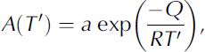
where T’ is the absolute temperature corrected for the dependence of the melting point on pressure (Reference PatersonPaterson, 1994), and a and Q are given by

(10, 11)

(12, 13)

The bedrock and surface topography compiled by Reference Letréguilly, Huybrechts and ReehLetréguilly and others (1991) is employed on a 20 km grid spacing using a polar stereographic projection. This topography dataset is distributed as part of the European Ice Sheet Modelling Initiative (EISMINT) for comparison of the Greenland ice sheet (coordinated by C. Ritz; see Reference HuybrechtsHuybrechts, 1998). The horizontal model domain spans 1640 ×2800 km² with a grid resolution of 20km in both horizontal coordinate directions (83 × 141 gridpoints). The vertical grid is divided equally into 30 levels. Different time-steps are employed for solving the dynamic evolution (At = 4.0years) and the thermodynamic evolution (At = 20.0years). The dynamics of the ice shelf and the grounding line are not included in the present model. The lateral boundary is decided by a floating condition by which any part of the ice sheet that floats due to its own buoyancy is immediately cut off. The geothermal heat flux for the boundary condition of thermodynamics is set at a constant value of 42 mW m–² throughout the experiments (Reference LeeLee, 1970). The ice enhancement factor is set at 3, and basal sliding is ignored. Changes in the elevation of the glacier bed under the load of the ice are calculated using an equation expressing the local isostatic rebound with a time constant of 3000 years (Reference Turcotte and SchubertTurcotte and Schubert, 1982). Monthly observed data compiled by Reference Calanca, Gilgen, Ekholm and OhmuraCalanca and others (2000) are used for the annual surface temperature, which is perturbed according to both the warming scenario and local surface elevation changes in terms of the prescribed lapse rate of 6.5 Kkm–¹. Computation took about 20 min per 50 kyr on a Hitachi SR8000 supercomputer.

The second part of the present model calculates the surface mass balance in two parts, accumulation and ablation, which are parameterized separately. Surface accumulation follows the present observation compiled by Reference Calanca, Gilgen, Ekholm and OhmuraCalanca and others (2000). It is assumed that there is no change in the accumulation distribution. Although ablation depends on the details of the energy balance at the ice-sheet surface, it is not possible to apply full energy-balance calculations over the entire model domain at every time-step. Therefore, ablation is parameterized by a simple function relating surface temperature to the ablation (the physical basis for this parameterization has been discussed by Reference OhmuraOhmura (2001)). The function in this paper assumes the following relation between summer temperature TJJA at the surface and ablation a _bl (in mmw.e. a^-1):

(14)

based on extensive observations in Greenland (Reference Ohmura, Wild and BengtssonOhmura and others, 1996). Equation (14) indicates that a _bl = 0 when T _JJA ≤ -2°C, and captures the observed features well. Ablation calculation requires the mean summer temperature or time series of surface temperature. In the present work, monthly observed data compiled by Reference Calanca, Gilgen, Ekholm and OhmuraCalanca and others (2000) were used for the reference temperature, which was then perturbed by warming and local elevation change. Most previous studies have used the positive-degree-day method (Reference Letréguilly, Huybrechts and ReehLetreguilly and others, 1991), and Reference SaitoSaito (2002) has discussed the difference between the two parameterizations. Although the results of the simulations using the two parameterizations differ, the main conclusion of this paper is not significantly affected.

3. Experiment and Results

The initial condition for the sensitivity studies was defined as the observed surface and bedrock topographies and an isothermal ice sheet. Using this initial condition, a simulation with fixed topography and free thermodynamics was conducted first under the present climate-forcing condition for 100 kyr. Then, using the final state of that simulation as the new initial condition, a further simulation with free topography was run for 100 kyr. The final state of this second simulation was then used as the initial condition for all sensitivity studies. Initial conditions were prepared using this model for each of the two numerical schemes.

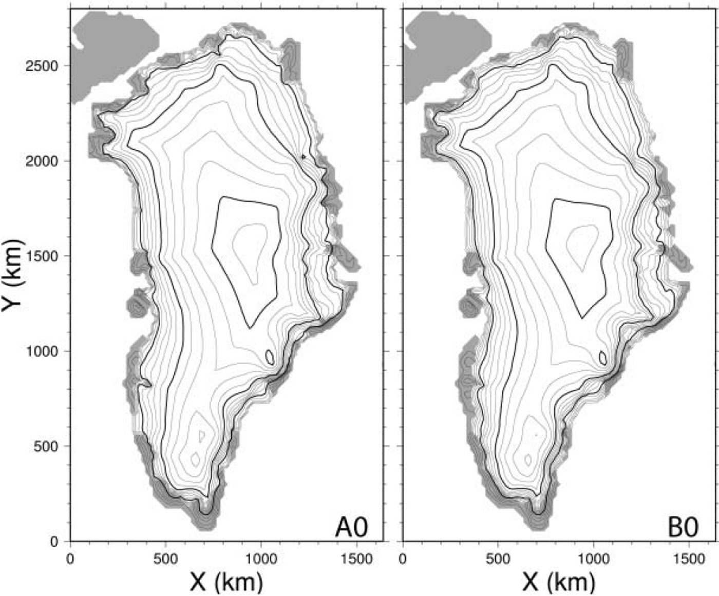
Uniform stepwise warming, where a spatially constant perturbation is applied suddenly to the initial condition, was adopted for all sensitivity studies. Experiments A and B were performed using the 9-point and 13-point scheme, respectively. A total of nine sensitivity experiments were conducted for each numerical scheme, with warming of +0, + 1 , . . . , + 8 K (referred to as experiments A0, A 1 , . . . , A8 etc.). All sensitivity studies were run for 50 kyr, sufficient to reach a steady state. Figure 2 shows the results for the control experiments A0 and B0. In both cases, the surface elevation (highest position) is well simulated compared to the observations. However, while the model simulates the observed features in the interior region quite well, the elevation (or thickness) near the margin is overestimated by 400m or more. The ice-sheet coverage is also overestimated by the simulation, which produces an overextension of the ice sheet at the northeast and southwest margins. Thus, the ice-sheet volume is also overestimated. The steady-state volumes indicated by A0 and B0 are 3.58 × 106 and 3.45 × 106 km , respectively, 38% and 33% higher than the present measured value of 2.6 × 106km (obtained from Reference Allison, Barry and GoodisonAllison and others, 2006).

Fig. 2.

Final state reached in the control experiments A0 (left) and B0 (right). Surface topography is shown in contour intervals of 200 m (thin) and 1000 m (thick), with ice-free land indicated by shading.

This overestimation is a common feature of many numerical simulations of the Greenland ice sheet (Reference Ritz, Fabre and LetréguillyRitz and others, 1997). Reference Ritz, Fabre and LetréguillyRitz and others (1997) concluded that a high ablation rate is necessary to obtain good agreement between the simulations and observations. However, other parameters may also have an effect. For example, ignoring basal sliding tends to produce thicker ice-sheet margins, and the presence of ice streams lowers the ice stiffness and increases the ice flux due to higher-order stress effects (not introduced under the shallow-ice approximation), basal sliding and larger strain heating. However, these effects cannot be represented in the present model. Unknown parameters such as geothermal heat flux or enhancement factors are also difficult to express as a single parameter for all of Greenland. Furthermore, the present ice sheet may not necessarily be in a steady state, and may in fact be in transition responding to past climate variability. All or some of these effects may cause an overall bias in the result. For the purposes of the present study, however, these overestimations are not important. Figure 3 shows the difference between the surface elevations reached in the final state (50 kyr) in the two control experiments A0 and B0 (B0 minus A0 is shown). As explained by Reference Hindmarsh and PayneHindmarsh and Payne (1996) using an isothermal ice-sheet model, the 13-point scheme gives a solution in which the surface elevation near the margin is lower, in this case by >200 m. On the other hand, the difference in interior regions is very small.

Fig. 3.

Difference between the surface topography of experiments B0 and A0 in the final state.

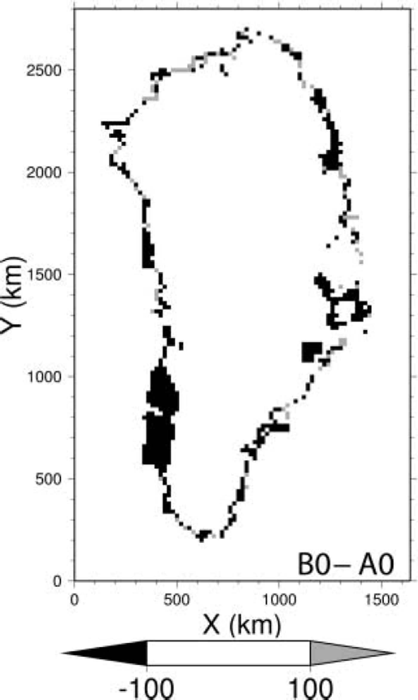
Figure 4 shows the final surface topography obtained by experiments A3 and A7. The response patterns of the Greenland ice sheet to uniform warming in both cases are generally similar, revealing a fragile region in the southwest between the two summits. The ice sheet separates into two parts under relatively small warming of 3K, while under higher forcing of around +5 K the southern part disappears entirely, leaving only the northern area. With further forcing, the northern region also begins to disappear, finally leaving only a small area on the higher mountains in the east. Although the mass-balance parameterizations differ, the results of this paper are comparable to those obtained in previous studies (Reference Letréguilly, Huybrechts and ReehLetréguilly and others, 1991).

Fig. 4.

Final results of A3 (left) and A7 (right), showing surface topography in contour intervals of 200 m (thin) and 1000 m (thick). Ice-free land is shaded.

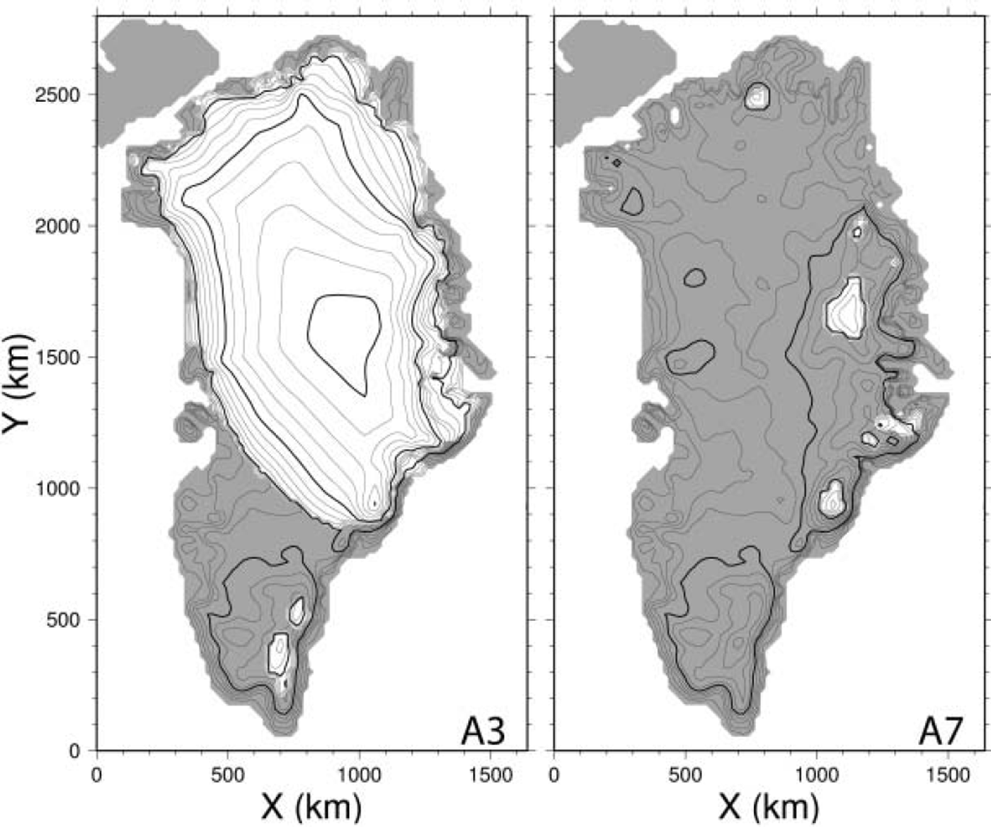
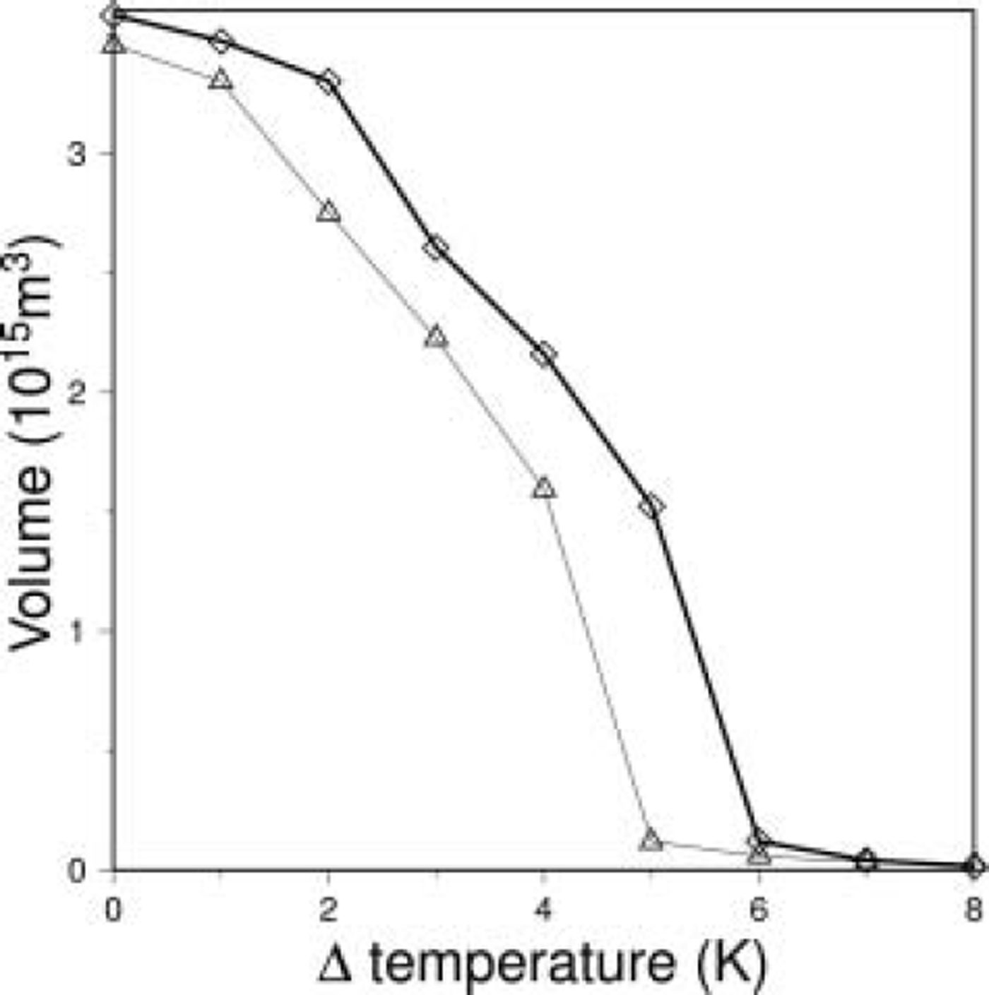
Figure 5 shows the final volume (50 kyr) obtained by these experiments. Although the volume change is modest for small temperature shifts, the gradient of volume decrease becomes steeper with increasing temperature shift. The gradient becomes steepest with 5 K warming, and almost all the ice melts with higher warming. However, while warming of 5 K results in a loss of approximately half the volume of the Greenland ice sheet in A5, the same warming causes most of the ice sheet to disappear in B5 (Fig. 6). The uncertainty of the temperature perturbation that causes most of the ice sheet to disappear is about 1 K.

Fig. 5.

Final volume change in response to warming scenarios. Thick and thin lines are the results of experiment A and B series, respectively.

Fig. 6.

Final result of 5 K warming for experiments A5 (left) and B5 (right), showing surface topography in contour intervals of 200 m (thin) and 1000 m (thick). Ice-free land is shaded.

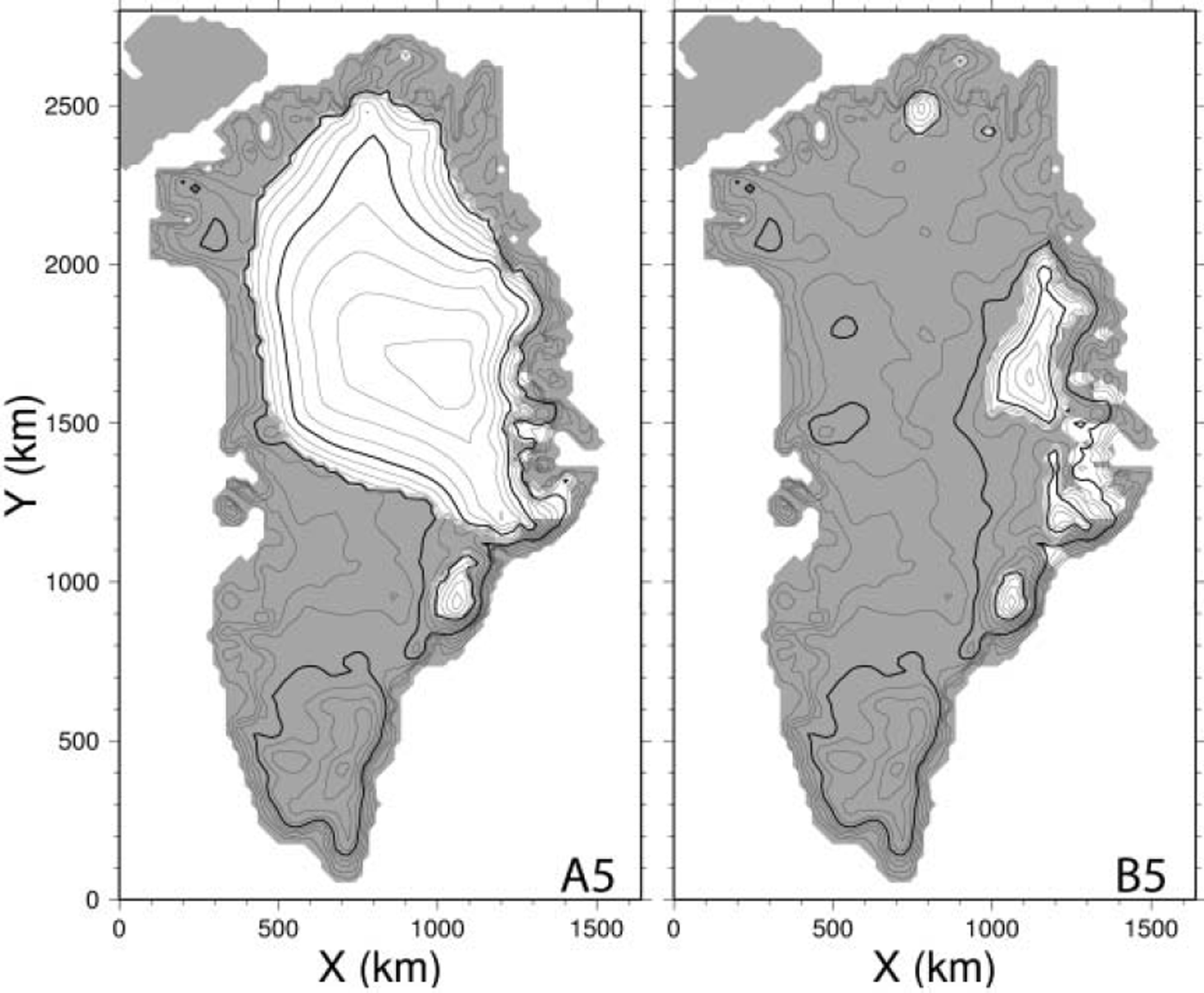
The major reason for the difference in the response is the difference between the two control experiments. As ablation is most where the elevation is lowest (e.g. the margin), the sensitivity to warming increases as the surface elevation decreases. As a result of elevation–ablation feedback, the higher margin in A0 compared to B0 offsets the simulated response by about 1 K.

The uncertainty evaluated in this paper is limited to models with horizontal resolution of 20 km. As explained by Reference Hindmarsh and PayneHindmarsh and Payne (1996) using an isothermal ice-sheet model, the solutions obtained by these two methods approach the exact solution from opposite sides at the high horizontal resolution employed here.

The volume–temperature diagram (Fig. 5) for the present Greenland ice sheet will shift leftwards (in the direction of lower temperature): As the elevation of the margin is overestimated in all of the cases examined in this study, the response will also be underestimated in all of the present cases. Moreover, the change in surface albedo due to the expansion of ice-free land may increase the sensitivity of the response. However, even if these processes are included in the model, a degree of uncertainty remains in either of these numerical analyses of the sensitivity of the ice-sheet volume to global warming.

4. Conclusion

The response of the Greenland ice sheet to global warming was evaluated using a three-dimensional ice-sheet model and two different numerical schemes in order to determine the sensitivity of the simulation to the numerical procedure employed. It was shown that the response of the Greenland ice sheet is influenced strongly by this difference in the numerical structure adopted for thickness evolution. In estimation of the contribution of ice-sheet melting to future sea-level rise, the steady state differs by as much as a factor of two under the same climate-change scenario (+5K in this study). Thus, the uncertainty in the temperature perturbation required for a certain volume change is about 1 K in the 2–5 K warming range. As the realistic range of future and past warming is within this range, careful interpretation of simulated volume change is required, and the adequacy of the numerical scheme employed should be considered in more detail. These topics will be addressed in future research.