

Introduction
The Nearctic leafhopper Scaphoideus titanus Ball (Hemiptera: Cicadellidae) was accidentally introduced in Europe in the 1950s (Bonfils and Schvester Reference Bonfils and Schvester1960; Schvester et al. Reference Schvester, Carle and Moutous1961). Southwestern and southern European grapevine growing areas were invaded before southeastern European regions that were colonised in the past decade only (Magud and Toševski Reference Magud and Toševski2004; Budinščak et al. Reference Budinščak, Križanac, Mikec, Seljak and Škorić2005; Zeisner Reference Zeisner2005; Der et al. Reference Der, Koczor, Zsolnai, Ember, Kolber and Bertaccini2007; Avremov et al. Reference Avremov, Ivanova and Laginova2011; Chireceanu et al. Reference Chireceanu, Ploaie, Gutue, Nicolae, Stan and Comsa2011). Currently, S. titanus occurs through most of southern Europe, from Portugal to Romania and Bulgaria, but the area of distribution is still expanding.
Scaphoideus titanus is the vector of the ‘Candidatus Phytoplasma vitis’, a Phytoplasma of the Elm Yellows or 16Sr-V group, an A2 quarantine pest for EPPO causing the Flavescence dorée (FD), an economically very important grapevine plant disease displaying a crisis-recovery-relapse cycle (European and Mediterranean Plant Protection Organization/Commonwealth Agricultural Bureau International 1996). In an area newly invaded by S. titanus, FD infestations follow with a time delay of several years if vector control measures are undertaken and less if not (Steffek et al. Reference Steffek, Reisenzein and Zeisner2007). Once present, the number of FD infected vine plants may increase tenfold every year and reach 80–100% within a few years, if no insect control is undertaken (European and Mediterranean Plant Protection Organization/Commonwealth Agricultural Bureau International 1996).
For these reasons, S. titanus control in FD uninfected vineyards and both S. titanus and FD control in FD-infected vineyards have become important components of vineyard pest management systems since the 1960s (Carle and Schvester Reference Carle and Schvester1964). In FD-infected areas, both the disease and the vector are usually subjected to compulsory control measures, including mandatory insecticide sprayings and mandatory uprooting of symptomatic vines and abandoned vineyards. Despite these measures, the FD is still spreading through southern Europe. In the last 10 years, new FD outbreaks have been reported from Serbia (Duduk et al. Reference Duduk, Botti, Ivanović, Krstić, Dukić and Bertaccini2004), Switzerland (Gugerli et al. Reference Gugerli, Besse, Colombi, Ramel, Rigotti and Cazelles2006), Slovenia (Seljak and Orešek Reference Seljak and Orešek2007), Portugal (De Sousa et al. Reference De Sousa, Casati, Cardoso, Baltazar, Durante and Quaglino2010), Romania (Irimia et al. Reference Irimia, Ulea and Balau2010), Croatia (Šeruga Musić et al. Reference Šeruga Musić, Škorić, Haluška, Križanac, Plavec and Mikec2011), and Austria (Reisenzein and Steffek Reference Reisenzein and Steffek2011).
Efficient management strategies and tactics target S. titanus densities and disease transmitting capacities by delaying the spread of FD infections, halting an ongoing FD epidemics and retarding an FD relapse. To increase the efficiency of S. titanus control, Rigamonti et al. (Reference Rigamonti, Jermini, Fuog and Baumgärtner2011) took into account the univoltine development and designed a phenology model simulating the successive occurrences of egg hatching, of nymphal instar presence and adult emergence. From the standpoint of supervised pest control, the model became a useful tool for the adaptive management of populations inhabiting vineyards in southern Switzerland (Jermini et al. Reference Jermini, Trivellone, Cara and Baumgärtner2013; Prevostini et al. Reference Prevostini, Taddeo, Balac, Rigamonti, Baumgärtner and Jermini2013). The focus on the period from egg hatching to adult emergence takes into account an important part of the dynamics of S. titanus but has limitations when seeking better insight into within- and between-generation processes to design integrated pest management systems on solid ecological ground. Specifically, the model by Rigamonti et al. (Reference Rigamonti, Jermini, Fuog and Baumgärtner2011) excludes diapause development of overwintering eggs as well as adult survival and reproduction.
The scope of this paper is to design, parametrise, and validate an age-structured multigeneration model representing multiannual infestation patterns of S. titanus populations. The model is based on theories on poikilothermic development and age-structured population dynamics that determine the explicative properties of the model. Field observations and published data provide the basis for model parameter estimation. Since the purpose of the model is to represent multiannual infestation patterns, model validation procedures test the model's predictive capabilities by comparing simulated patterns with long-term grapevine plant infestation data. In addition, the sensitivity of the final output to model parameter changes is tested for guiding future research work.
Methods
Scaphoideus titanus is a univoltine species whose individuals pass through different life stages according to the insect poikilothermic development mode in temperate countries: the eggs hatch in spring and the egg stage is followed by five nymphal instars that, in summer, develop into adults. Eggs overwinter in diapause, which is a state of low activity associated with reduced morphogenesis, increased resistance to environmental extremes, and altered or reduced behavioural activity, mediated by hormones (Nechols et al. Reference Nechols, Tauber, Tauber and Masaki1999). Diapause is mainly but not exclusively controlled by a combination of temperature and photoperiod (Tauber and Tauber Reference Tauber and Tauber1976; Tauber et al. Reference Tauber, Tauber and Masaki1986; Leather et al. Reference Leather, Walters and Bale1993; Nechols et al. Reference Nechols, Tauber, Tauber and Masaki1999). Nevertheless, we focus on temperature as driving variable for diapause development.
In the present model, the development of S. titanus has been divided into four morphologically and physiologically different life stages (nymphs, adults, diapausing eggs, post-diapausing eggs). To facilitate model description and provide easy access to the supportive literature, the following methodological sections briefly refer to (1) stochastic cohort development, (2) poikilothermic cohort development with model parameter estimation, (3) simulation model development, (4) validation, and (5) sensitivity probe.
Stochastic cohort development
If the variability in developmental time is high relative the mean developmental time, a stochastic model may be appropriate to model cohort development (Di Cola et al. Reference Di Cola, Gilioli and Baumgärtner1999). The time-varying distributed delay of Vansickle (Reference Vansickle1977) is applied to model the development of S. titanus nymphs (j = 1), adults (j = 2), diapausing eggs (j = 3), and post-diapausing eggs (j = 4). Manetsch (Reference Manetsch1976), Plant and Wilson (Reference Plant and Wilson1986), Di Cola et al. (Reference Di Cola, Gilioli and Baumgärtner1999), and Severini (Reference Severini2009) contributed to the development of the distributed delay theory in an ecological context. In Manetsch's (Reference Manetsch1976) and Vansickle's (Reference Vansickle1977) notation, the model applied to the j-th life stage is represented by:
 $$ no{ {\frac{{d{{r}_{ji}}(t)}}{{dt}}\, = \,\frac{{{{k}_j}}}{{DE{{L}_j}(t)}}\left\bigg[ {{{r}_{ji\,{\rm{ - }}\,1}}(t)}\, \right }\cr \qquad\qquad\left {\rm{ - }}\,{{r}_{ji}}(t)\left( {{\rm{1}}\, + \,A{{R}_j}(t)\frac{{DE{{L}_j}(t)}}{{{{k}_j}}}\, + \,\frac{{d\,DE{{L}_j}(t)}}{{{{k}_j}dt}}} \right)} \right] \cr (1)$$
 $$j\, = \,{\rm{1,}}\,{\rm{2,}}\,{\rm{3,}}\,{\rm{4}}$$
 $$i\, = \,{\rm{1,}}\,{\rm{2,}} \ldots {\rm{, }}\ {{k}_j}{}$$
where t is time (days), rji (t) is the transition rate of the i-th substage in the j-th life stage, kj is the number of delay substages in the j-th life stage, DELj (t) is the time dependent developmental time (days) in absence of losses in the j-th life stage, and ARj (t) is the time dependent proportional changes or attrition in the j-th life stage. In the case under study, the entry rate r 11(t) into the nymphal stage is represented by an initialisation function in the first year and by the exit rate of the post-diapausing eggs in the succeeding years. The exit rate of the nymphal stage becomes the entry rate r 21(t) into the adult stage; the oviposition is the entry rate r 31(t) into the diapausing eggs stage, whose exit rate is the entry rate r 41(t) into post-diapausing egg development.
According to Manetsch (Reference Manetsch1976) and Vansickle (Reference Vansickle1977), the occurrence Qj (t) of each life stage can be obtained from
 $${{Q}_j}(t)\, = \,\mathop{\sum}\limits_{i\, = \,{\rm{1}}}^{{{k}_j}} {\frac{{DEL{{\,}_j}(t)}}{{{{k}_j}}}\,{{r}_{ji}}(t)} \eqno (2)$$
For constant conditions, Vansickle (Reference Vansickle1977) defines the relationships between kj , DELj and ARj as follows:
 $$ {{k}_j}\, = \,\frac{{{\rm{\rmu }}_{j}^{{\rm{2}}} }}{{s_{j}^{{\rm{2}}} }} \eqno (3\rm {a})$$
 $$DE{{L}_j}\, = \,{{{\rm{\rmu }}}_j}\,{{{\rm{{\repsilon}}}}_j}^{{\left( {{\rm{ - }}\,\frac{{\rm{1}}}{{{{k}_j}}}} \right)}} \eqno (3\rm {b})$$
 $$A{{R}_j}\, = \,{{k}_j}\left[ {\frac{{\rm{1}}}{{{{{\rm{\rmu }}}_j}}}\,{\rm{ - }}\,\frac{{\rm{1}}}{{DE{{L}_j}}}} \right]\eqno (3\rm {c})$$
where μ j is the observed developmental time, sj 2 is the variance, and ε j is the stage-specific survival.
Poikilothermic cohort development
Developmental rates and variance. Between the stage-specific lower j Tl and the upper j Tu thresholds, the developmental rate zj (T) of nymphs and diapausing eggs, and the senescence rate of adults is represented by the curvilinear model of Brière et al. (Reference Brière, Pracros, Le Roux and Pierre1999). However, a linear model is used to describe the developmental rate of post-diapausing eggs above the lower and below the upper thresholds; if 4 Tl > T > 4 Tu , the rate z4 (T) is equal to 0.001:
 $$ no {{\rm{0}}{\rm{.01}}\!\leq {{z}_j}(T)\, = &\,{{{\rm{\alpha }}}_j}\,T\,(T\,{\rm{ - }}\,{\pre}^{j}{{T}_l})\,{{\left( {{\pre}^{j}{{T}_u}\,{\rm{ - }}\,T} \right)}^{{{{\rm{\rbeta }}}_j}}} \; \; \; \; \cr &{\rm{for}}\ j\, = \,{\rm{1,}}\,{\rm{2,}}\,{\rm{3}} (4\rm{a}) \eqno $$
 $$ no {{\rm{0}}{\rm{.001}}\!\leq {{z}_j}(T)\, = \,{{{\rm{\alpha }}}_j}(T\,{\rm{ - }}\,{\pre}^{j}{{T}_l})\; \; \; \; {\rm{for}}\ {}j\, = \,{\rm{4}} (4{\rm b})\eqno $$
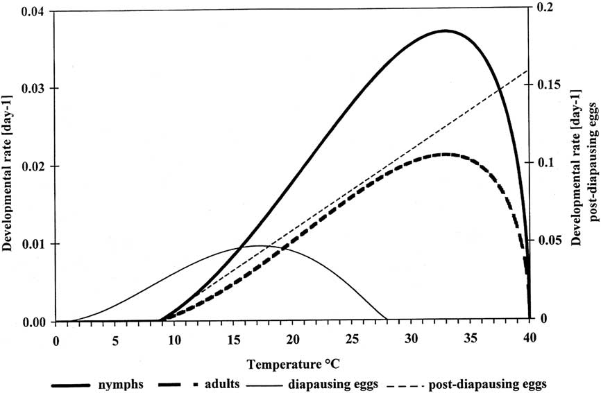
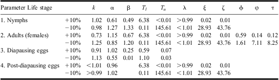
where α j and β j are parameters. For nymphs and post-diapausing eggs, the estimation procedures and the values for α j , β 1 , j Tl , j Tu are given in Rigamonti et al. (Reference Rigamonti, Jermini, Fuog and Baumgärtner2011). For adults, Bressan et al. (Reference Bressan, Girolami and Boudon-Padieu2005) provide data on the senescence rate and associated variance at 26 °C; at temperatures different from 26 °C, the senescence rate is assumed to be proportional to the developmental rate of nymphs (Table 1). Post-diapause development time of eggs was estimated to be 196.6-day degrees above the lower and below the upper thresholds (Rigamonti et al. Reference Rigamonti, Jermini, Fuog and Baumgärtner2011). The inverse of 196.6 is equal to α4 reported in Table 1. For diapausing eggs, the development rate parameters α3, β3 3 Tl , and 3 Tu were calculated as follows.
Parameter estimates for the time varying distributed delay-based model simulating the pluriannual infestation patterns of Scaphoideus titanus on grapevine plants, with reference to the relevant equations detailed in the text

aObtained from Rigamonti et al. (Reference Rigamonti, Jermini, Fuog and Baumgärtner2011).
bObtained in this paper from field experiments.
cObtained from expert opinions.
dObtained from Bressan et al. (Reference Bressan, Girolami and Boudon-Padieu2005).
na = not applicable.
To initialise the model, a cumulative Weibull frequency distribution was fitted to the normalised egg hatching data observed in cages set up in 2008 in a vineyard located at Contone, southern Switzerland (Rigamonti et al. Reference Rigamonti, Jermini, Fuog and Baumgärtner2011). The post-diapause development time of 196.6 day-degrees and the Weibull frequency distribution given in Rigamonti et al. (Reference Rigamonti, Jermini, Fuog and Baumgärtner2011) allow the calculation of the calendar days on which 0.1%, 25%, 50%, 75%, and 99.9% of egg groups terminated diapause in 2008. The below described simulation model was used to calculate the cumulative oviposition patterns and obtain the calendar days on which 0.1%, 25%, 50%, 75%, and 99.9% of egg groups entered diapause in the preceding year (2007). For each of the five groups, the duration (days) from diapause entry to diapause termination can be computed. Importantly, for each group the respective rate sum detailed by Curry and Feldman (Reference Curry and Feldman1987) can be calculated. Accordingly, the fraction dt of the mean development that has occurred after D days is:
 $${{d}_t}\, = \,\frac{{\rm{1}}}{n}\mathop{\sum}\limits_{s\, = \,{\rm{1}}}^{nD} {z({{T}_s})} \eqno (5)$$
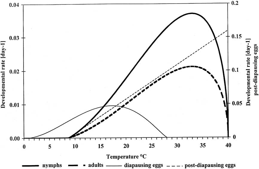
where n = 24 time increments per day, Ts is the discrete environmental temperature measurements for the s-th time increment obtained at the nearby Magadino weather station, nD is the number of increments in D days. Once dt is equal to 1 the development of a life stage is completed. Using initially α1 for α3, different combinations of β3, 3 Tl and 3 Tu produced different group means and variances. The smallest coefficient of variability among the group means yielded the estimates for β3, 3 Tl and 3 Tu , while α3 was finally obtained by equating the sum of equation [4a] equal to 1. The parameter values for the stage-specific developmental rates for all life stages are given in Table 1, while the response to temperature is depicted in Figure 1.
Illustration of temperature-dependent developmental rates for diapausing eggs, post-diapausing eggs, nymphs, and senescence rates of adults of the grape leafhopper Scaphoideus titanus. In the temperature range delimited by the lower and upper thresholds a linear model was applied to post-diapausing eggs, while the curvilinear model of Brière et al. (Reference Brière, Pracros, Le Roux and Pierre1999) was used for all other life stages (the parameter estimates are given in Table 1, the developmental rates below and above the thresholds are given in the text).
The estimates for kj have been obtained from the literature or expert opinions. Specifically, the experiments of Rigamonti et al. (Reference Rigamonti, Jermini, Fuog and Baumgärtner2011) and the data reported by Bressan et al. (Reference Bressan, Girolami and Boudon-Padieu2005) provide a series of means and variances in development times for nymphs as well as senescence of adult females, respectively. The mean ratio of the squared means to the variance given in equation [3a] is used to estimate for kj . For diapausing and post-diapausing eggs, however, expert opinion was considered for setting the values to 25 (Table 1).
Survivorship. All life stages except diapausing eggs are affected by intrinsic mortality and low temperatures. Nymphs and adults survival is also affected by a lack of food during grapevine plant dormancy. The stage specific intrinsic survival ε j in equation [3b] is tentatively set to 1 for diapausing eggs and represented by a Beta distribution for the other life stages:
 $$no {{\rm{0}}{\rm{.001}}\!\leq {{{\rm{{\repsilon}}}}_j}\left( T \right)\, = &\,{{{\rm{\rlambda }}}_j}\,{{\left( {T\,{\rm{ - }}\,{\pre}^{j}{{T}_{l}}}} \right)}^{{{{\rm{\rxi }}}_j}}} \,{{\left( {{\pre}^{j}{{T}_u}\,{\rm{ - }}\,T} \right)}^{^{{{{{\rm{\rvarsigma }}}_{_{j} }}}} }} \; \; \; \; \cr &{\rm{for}}\ {}j\, = \,{\rm{1,}}\,{\rm{2,}}\,{\rm{4}} (6{\rm a})$$
 $${{{\rm{{\repsilon}}}}_j}(T)\, = \,{\rm{1}}{\rm{.0}}\; \; \; \; {\rm{for}}\ j\, = \,{\rm{3}}\eqno (6{\rm b})$$
where λ j , ξ j and ζ j are parameters that were estimated on the basis of expert opinions regarding the shape and the level of survivorship between the lower and upper thresholds, assumed to correspond to the respective development thresholds (Table 1).
For the cultivar Pinot noir, Wermelinger et al. (Reference Wermelinger, Candolfi and Baumgärtner1992) reported bud break once 35.8 day-degrees have been accumulated after 1 January above the 10 °C threshold for plant development. In southern Switzerland, the beginning of leaf discolouration is generally observed around Julian day 290. Between this day and bud break in the succeeding year, the plant is assumed to be dormant causing a proportional daily loss rate of μ p = 0.5 among nymphs and adults.
Temperatures below the lower developmental threshold j Tl are responsible for a proportional loss rate of 0.75 < μ T = 0.75 (1.0–0.1149T) for all life stages except diapausing eggs. Expert opinion was considered in the estimation of μ p and μ T . The loss rates μ p and μ T are added to the attrition term ARj (t) of equation [1].
Oviposition. According to Curry and Feldman (Reference Curry and Feldman1987), the reproduction rate for the i-th instar is the product of the reproductive profile fi , i.e. the relative age-specific fecundity rate in the i-th substage, and the temperature-dependent reproductive potential F(T), i.e. the total number of eggs laid by a female conditioned on her living throughout the oviposition period. To represent fi , we make use of the information provided by Schvester et al. (Reference Schvester, Moutous and Carle1962), Vidano (Reference Vidano1964), and Bressan et al. (Reference Bressan, Girolami and Boudon-Padieu2005) indicating that females pass through a 10 days pre-reproductive period (corresponding to i = 1, 2), a 10 days reproductive period (corresponding to i = 3, 4), to that we tentatively add a 60 days post-reproductive phase (corresponding to 4 < i ≤ 8). For each substage in the reproductive period (i = 3, 4), the relative age-specific fecundity rate per day is 0.5 and 0 otherwise. To obtain F(T) we first calculate the relative reproductive potential m(T) as:
 $$\quad\quad\quadno {m(T)\, = &#x0026;\,{\rm{\rvarphi }}\,{{\left( {T\,{\rm{ - }}\,{\pre}^{{\rm{2}}}{{T}_l}} \right)}^\rphi } \,{{\left( {{\pre}^{{\rm{2}}}{{T}_u}\,{\rm{ - }}\,T} \right)}^{\rm{\rtau }}} \; \; \; \; \cr &#x0026;{\rm{for}}{{\ }^{\rm{2}}} {{T}_l}\,{\rm{ \lt }}T\,{\rm{ \lt }}\,{{}^{\rm{2}}} {{T}_u}{\rm{,}} \quad\quad\quad\quad\ (7)$$
with m(T) = 0 for T ≤ 2 Tl or T ≥ 2 Tu . The estimates for the parameters φ, ϕ and τ are based on expert opinion on temperature effects on fecundity. To obtain F(T),m (T) is multiplied by the total number of 14.58 eggs per female laid at 26 °C (Bressan et al. Reference Bressan, Girolami and Boudon-Padieu2005). Subsequently, the sum of the products fi F(T) over the 3rd and 4th substage is related to the daily aging process and multiplied by the occurrence of females, that is Q 2(t) of equation [2] times the sex ratio of 0.5 (Curry and Feldman, Reference Curry and Feldman1987). The estimates for the parameters of equation [7] are given in Table 1.
Simulation model development
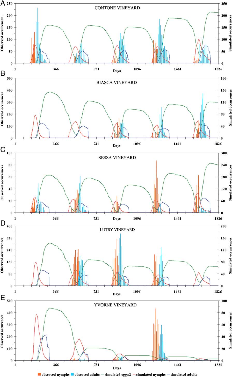
Manetsch (Reference Manetsch1976) and Abkin and Wolf (Reference Abkin and Wolf1976) describe the methodology for discretising equation [1] to simulate a delay process where losses, accretions, and delay length varies over time. To assure stability and nonnegative flow rate, a time increment Δt of 1 hour was adequate. In each time increment, the mean temperature is calculated by forcing a cosine function through daily temperature minima and maxima measured at locations and during years of interest (Bianchi et al. Reference Bianchi, Baumgärtner, Delucchi and Rahalivavololona1990). Curry and Feldman (Reference Curry and Feldman1987) explain in detail how to incorporate discrete environmental temperature measurements Ti into survival and development functions. The model is initialised with a cumulative input equal to 100 obtained from the Weibull function. For each time increment, instantaneous values for μ j , ε j and DELj of equation 3a, 3b, 3c are calculated. Likewise, instantaneous mortality and oviposition rates are computed. The model written in the Pascal programming language calculates the daily occurrences of diapausing eggs, post-diapausing eggs, nymphs, and adults that appear as outputs in Figures 2 and 3.
The simulated (lines) and observed (bars) occurrences of Scaphoideus titanus life stages on grapevine plants in vineyards located in southern and western Switzerland (A: Contone vineyard, B: Biasca vineyard, C: Sessa vineyard, D: Lutry vineyard, E: Yvorne vineyard). Occasional data were obtained in a monitoring program carried out in FD free zones. The nymphs were obtained through the beating tray method, while yellow sticky traps yielded information on adult presence. The simulated egg occurrences correspond to literature information mentioned in the text. Note that in Figure 2B the observed nymph occurrences are multiplied by ten. Note also that in the Sessa vineyard in 2008 and 2009 adult monitoring was discontinued in the early summer.

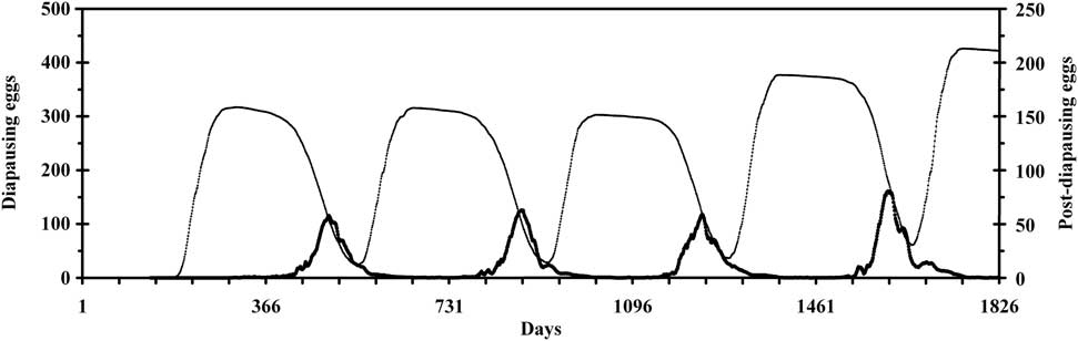
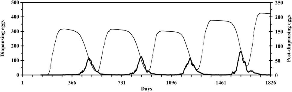
The simulated occurrences of Scaphoideus titanus diapausing (thin line) and post-diapausing (thick line) eggs on grapevine plants in the Contone vineyard (southern Switzerland).
To illustrate the application of time distributed delay simulation models in ecology, the reader is referred to Welch et al. (Reference Welch, Croft, Brunner and Michels1978); Fouque and Baumgärtner (Reference Fouque and Baumgärtner1996), Gutierrez (Reference Gutierrez1996), Di Cola et al. (Reference Di Cola, Gilioli and Baumgärtner1999), Wearing et al. (Reference Wearing, Rohani, Cameron and Sait2004), Samietz et al. (Reference Samietz, Graf, Höhn, Schaub and Höpli2007), Arthur et al. (Reference Arthur, Yang and Wilson2011), and Gutierrez et al. (Reference Gutierrez, Ponti, Cooper, Gilioli, Baumgärtner and Duso2012), for example.
Model validation
In agreement with the purpose of the model (Rykiel Reference Rykiel1996), predicted infestation patterns were visually compared with long-term data on infestation patterns in several vineyards. The model produces, distributed over the simulation time period, infestation relative to the initial input. The dynamics of these infestations represent here the calculated infestation patterns.
Over a period of five years, from 2006 to 2010, nymph and adult occurrences were occasionally monitored in five vineyards located in western Switzerland (Yvorne, Lutry) and southern Switzerland (Contone, Biasca, Sessa). The vineyards are located in FD-free zones. Data on nymphs were obtained through the beating tray method, while yellow sticky traps yielded information on adult presence. The details on the sampling technique have been reported in a previous paper (Rigamonti et al. Reference Rigamonti, Jermini, Fuog and Baumgärtner2011). These counts taken through time represent here the observed infestation pattern.
The daily maximum and minimum temperatures for the vineyards during the period under study were approximated by using the recordings of the Swiss Federal Office of Meteorology and Climatology (MeteoSwiss) made at the Aigle, Pully, Magadino, Comprovasco, and Lugano stations, respectively.
Sensitivity probe
The variation in the output of the model, restricted to the occurrence of diapausing eggs on the last day of the five years simulation period, is apportioned to a 10% change in the estimates of the parameters listed in Table 1, with the exception of the fecundity that is tested through the parameter φ. Since the development of all nondiapausing life stages is constraint by the same upper and lower thresholds, the 10% change is simultaneously applied to post-diapausing eggs, nymphs, and adults. The test consists in changing one-factor-at-a-time. The results are expressed as relative occurrences (RO), i.e. as occurrences relative to the occurrences obtained in the standard model with the parameter estimates given in Table 1.
Results and discussion
The temperature dependencies of stage-specific developmental and senescence rates between the lower and upper thresholds are illustrated in Figure 1. For nondiapausing life stages, the lower threshold of 8.7 °C reported in Table 1 is slightly lower than the threshold of 10 °C for plant development (Wermelinger et al. Reference Wermelinger, Baumgärtner and Gutierrez1991, Reference Wermelinger, Candolfi and Baumgärtner1992). Remarkably, the developmental rates of diapausing eggs are lower, and the curve is shifted to a lower temperature range than observed for post-diapausing eggs, nymphs, and adults (Table 1). The shifting of the developmental and the concomitant reduction of the lower and upper temperature thresholds have been hypothesised for and observed in many diapausing insects, including the corn earworm Helicoverpa zea (Boddie) (Lepidoptera: Noctuidae) (Logan et al. Reference Logan, Stinner, Rabb and Bacheler1979) and the European grape moth Lobesia botrana (Denis and Schiffermüller) (Lepidoptera: Tortricidae) (Baumgärtner et al. Reference Baumgärtner, Gutierrez, Pesolillo and Severini2012). Noteworthy, the developmental rate of diapausing eggs at 20 °C is much higher than at 5 °C, as reported by Chuche and Thiery (Reference Chuche and Thièry2012).
The model is built on the basis of poikilothermic cohort development, with temperature-dependent developmental rate, survival, and fecundity functions, treated by Curry and Feldman (Reference Curry and Feldman1987); the diapause theory conceptualised by Nechols et al. (Reference Nechols, Tauber, Tauber and Masaki1999); and stochastic development of age-structured populations according to Plant and Wilson (Reference Plant and Wilson1986), Gutierrez (Reference Gutierrez1996), and Di Cola et al. (Reference Di Cola, Gilioli and Baumgärtner1999). A model built on these basic elements has, in our view, satisfactory explicative qualities.
According to Rykiel (Reference Rykiel1996) the purpose of the model is decisive for validation procedure selection. A monitoring program for supervised management of S. titanus made available occasional data from several vineyards. In this program, the monitoring of nymphs was discontinued once adults appeared in sticky traps. No attempt was made to record egg hatching in winter and no data were collected in the presence of diapausing eggs. Moreover, sticky trap catches of adults are affected by weather conditions. These limitations affect the model predictions and field observation comparisons. However, for the purpose of the work, which is the representation of multiannual infestation patterns, the available monitoring information appears to be sufficient for model validation (see subsequent section). A model designed for representing population densities, however, would require more reliable data for validation, changes in model input and a possible revision of mortality functions. Moreover, such a model should include dispersal including the passage of young nymphs through the vineyard floor vegetation (Trivellone et al. Reference Trivellone, Baumgärtner, Linder, Cara, Delabays and Jermini2011).
According to Figures 2A–2E, the model generally represents the observed five years infestation pattern at the five locations in a satisfactory manner. Specifically, the correspondence between field observations and the predicted occurrences of nymphs, the presence of adults, and the appearance of the combined diapausing and post-diapausing eggs is adequate. The simulated egg deposition period coincides with the occurrence of gravid females observed by Cravedi et al. (Reference Cravedi, Mazzoni and Cervato1993) in northern Italian vineyards. The duration of adult presence is also satisfactorily represented by the model, while the predicted nymph occurrence lasts for a longer time period then observed in the field.
The model predicts the beginning of diapause termination as early as in October and the continuing termination of diapause for a small number of eggs throughout the winter. However, the survival of post-diapausing eggs is negatively affected by low winter temperatures. Nymphs not only suffer from the effect of low temperatures but also from a lack of food prior to bud break. In mild winters and at locations with frequent temperatures between 5 °C and 10 °C the plant dormancy effect is particularly high. Under these conditions, the disruption of the phenological synchrony between S. titanus and the plant could have a significant effect on infestation patterns. Importantly, the model predicts an overlapping in the occurrence of newly laid eggs and diapausing eggs from the previous year. As a result, diapausing eggs are always present in the vineyards (Fig. 3).
Since here the developed model adequately represents the data in FD uninfested vineyards, it is qualified with satisfactory predictive qualities and assumed to hold the promise for further improve adaptive management of S. titanus populations (Jermini et al. Reference Jermini, Trivellone, Cara and Baumgärtner2013; Prevostini et al. Reference Prevostini, Taddeo, Balac, Rigamonti, Baumgärtner and Jermini2013).
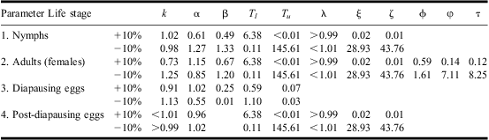
Table 2 shows the RO of diapausing eggs on the last day of the five years simulation period in response to a 10% changes in parameter values. Accordingly, the model output is most sensitive to changes in the upper threshold ( J Tu ) and in the shape parameters (ξ J and ζ J ) of the beta distribution for the temperature-dependent survivorship. On the other hand, the model is least sensitive to the 10% variation in the shape parameter of the development function (kJ ) and the level of survivorship λ J . The small variation of RO in response to the shape parameter (kJ ) of the development function and the level of survival (λ j ) was not expected, considering the importance given to those parameters in traditional life table studies. Apparently, the model is sensitive to 10% changes in parameters whose estimates are based on expert opinions rather than experimentation (Table 1). Sensitivity analysis is the study of how the uncertainty in the output of a mathematical model or system can be apportioned to different sources of uncertainty in its inputs (Saltelli et al. Reference Saltelli, Ratto, Andres, Campolongo, Cariboni and Gatelli2008). Since in our case experts did not provide any information on uncertainties, the sensitivity study deals with parameter estimates with both known and unknown reliability. Therefore, we refrained from conducting a comprehensive sensitivity analysis, including the changing of more than one-factor-at-a-time, and limit the work to a sensitivity probe providing guidance for future research to increase the robustness of the model. For example, experimental work on high temperature effects on development and survival may yield parameters estimates with uncertainties.
Results of the sensitivity probe, which yields the RO of diapausing eggs on the last day of the five years simulation period in response to 10% changes in model parameters (RO refers to the occurrence of diapausing eggs in relation to the standard model with parameter estimates given in Table 1; since the same upper ( j Tu ) and lower ( j Tl ) developmental thresholds have been used for all non-diapausing life stages, the respective sensitivity test is carried out simultaneously for eggs, nymphs, and adults)
RO, relative occurrence.
The model estimates and the field observations indicate similar infestation patterns at all locations (Figs. 2A–2D) with the exception of Yvorne (Fig. 2E). The predicted decreasing infestation levels in the Yvorne vineyard (Fig. 2E) is in contrast to the respective field observations. Presumably, the discrepancy between predictions and observations is due to the use of unrepresentative weather data from the distant and topographically differently positioned Aigle station. From the response of the predicted infestation patterns to relatively cooler climates, as apparently in the case of the Aigle data, we conjecture that S. titanus is approaching the northern limit for distributions (Rigamonti et al. Reference Rigamonti, Trivellone, Jermini and Baumgärtner2013). Since the species extends through the United States of America into Canada (Commonwealth Agricultural Bureau International 1992), a critical evaluation of this result is a prerequisite for sketching out the possible area of distribution in Europe. Such a project may benefit from the weather data bank of Yang et al. (Reference Yang, Wilson and Wang2010) and the methodology used by Gutierrez et al. (Reference Gutierrez, Ponti, Cooper, Gilioli, Baumgärtner and Duso2012) to assess the invasive potential of L. botrana in North America.
The Weibull input function as well as the developmental rate function of diapausing eggs have been parametrised, and the model has been validated in a narrow range of ecological conditions relative to the inhabited zones in North America and Europe (Commonwealth Agricultural Bureau International 1992). To extend the applicability of the model, it may be necessary to account for other environmental factors than temperature such as humidity and photoperiod. In particular, the diapause theory predicts that diapause is mainly but not exclusively controlled by a combination of temperature and photoperiod (Tauber and Tauber Reference Tauber and Tauber1976; Tauber et al. Reference Tauber, Tauber and Masaki1986; Leather et al. Reference Leather, Walters and Bale1993; Nechols et al. Reference Nechols, Tauber, Tauber and Masaki1999).
Acknowledgements
The Swiss Federal Office of Meteorology and Climatology (MeteoSwiss), Zurich, Switzerland, kindly made available weather data from the Aigle, Pully, Magadino, Comprovasco, and Lugano stations. The technical assistance of Drs. Silvia Bellion, Silvia Salini, and Alessio Pavarino is greatly appreciated. The authors are grateful to anonymous reviewers for comments leading to substantial improvements of the paper.