




1 Introduction
The challenge to describe the physics of turbulent flows comes not only from the wide range of scales involved, but also from the spatial organization of the flow, which is responsible for the coupling between scales (Monin & Yaglom Reference Monin and Yaglom1975; Frisch Reference Frisch1995; Pope Reference Pope2000). One manifestation of this complex structure is the emergence of tubes, where the magnitude of the vorticity vector  $\unicode[STIX]{x1D74E}=\unicode[STIX]{x1D735}\times \boldsymbol{U}$ is very high (Siggia Reference Siggia1981; Douady, Couder & Brachet Reference Douady, Couder and Brachet1991; Jimenez et al. Reference Jimenez, Wray, Saffman and Rogallo1993; Ishihara et al. Reference Ishihara, Kaneda, Yosokawa, Itakura and Uno2007; Buaria et al. Reference Buaria, Pumir, Bodenschatz and Yeung2019). The amplification of vorticity results from its nonlinear coupling with the rate-of-strain tensor,
 $\unicode[STIX]{x1D668}=\frac{1}{2}(\unicode[STIX]{x1D662}+\unicode[STIX]{x1D662}^{\text{T}})$, where
 $\unicode[STIX]{x1D662}=\unicode[STIX]{x1D735}\boldsymbol{U}$ is the velocity gradient tensor (Frisch Reference Frisch1995; Tsinober Reference Tsinober2009).
Much of the experimental investigation of turbulent flows has relied on the investigation of the velocity structure functions, defined as the moments of the difference between the component of flow velocity,  $\boldsymbol{U}$, at two spatial points separated by a distance
 $\boldsymbol{x}$ along a spatial direction (say
 $x$):
 $D_{n}(x)=\langle (U(x)-U(0))^{n}\rangle$. While this quantity, defined with the help of two spatial points, is accessible from wind tunnel experiments (Comte-Bellot & Corrsin Reference Comte-Bellot and Corrsin1966; Pope Reference Pope2000; Bodenschatz et al. Reference Bodenschatz, Bewley, Nobach, Sinhuber and Xu2014) and provides a very useful characterization of the scaling properties of the flow, it does not provide much information on the structural aspects of the velocity field. This deficiency is particularly important in the context of modelling the energy flux acting at small scales below the filtering scale in a large-eddy simulation approach (Borue & Orszag Reference Borue and Orszag1998; Tao, Katz & Meneveau Reference Tao, Katz and Meneveau2002; Van der Bos et al. Reference Van der Bos, Tao, Meneveau and Katz2002; Meneveau Reference Meneveau2011; Johnson & Meneveau Reference Johnson and Meneveau2018). A possible approach to studying simultaneously the structural and the scaling aspects of turbulence consists in considering the velocity at four points separated by a distance
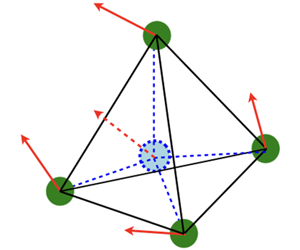
 $R_{0}$ forming a regular tetrad (Chertkov, Pumir & Shraiman Reference Chertkov, Pumir and Shraiman1999). How such a tetrad deforms as the fluid particles move with the flow reveals interesting properties of the flow (Pumir, Shraiman & Chertkov Reference Pumir, Shraiman and Chertkov2000; Biferale et al. Reference Biferale, Boffetta, Celani, Devenish, Lanotte and Toschi2005; Naso & Pumir Reference Naso and Pumir2005; Xu, Ouellette & Bodenschatz Reference Xu, Ouellette and Bodenschatz2008; Hackl, Yeung & Sawford Reference Hackl, Yeung and Sawford2011; Meneveau Reference Meneveau2011; Xu, Pumir & Bodenschatz Reference Xu, Pumir and Bodenschatz2011; Naso & Godeferd Reference Naso and Godeferd2012; Devenish Reference Devenish2013; Devenish & Thomson Reference Devenish and Thomson2013; Sawford, Pope & Yeung Reference Sawford, Pope and Yeung2013; Naso Reference Naso2019). Here, we focus on the perceived velocity gradient tensor (PVGT),
 $\unicode[STIX]{x1D648}$, obtained from the velocity differences over the distance between the four points defining the tetrad. The PVGT can be viewed as an extension of the velocity gradient tensor to length scales beyond the dissipation range (Chevillard & Meneveau Reference Chevillard and Meneveau2006; Meneveau Reference Meneveau2011; Jucha et al. Reference Jucha, Xu, Pumir and Bodenschatz2014; Johnson & Meneveau Reference Johnson and Meneveau2016; Xu, Pumir & Bodenschatz Reference Xu, Pumir and Bodenschatz2016). Other attempts to study the velocity gradient beyond the dissipative scale include the velocity gradient coarse-grained over a spherical volume following a fluid particle trajectory (Meneveau & Lund Reference Meneveau and Lund1994), and the velocity gradient obtained from the velocities of fluid particles within a sphere centred at a target fluid particle (Lüthi et al. Reference Lüthi, Ott, Berg and Mann2007). As we stress in this work, the study of the PVGT provides some information on the relative role of vorticity and strain as a function of scales, and also on their dynamics.
As shown, for example, by Pumir, Bodenschatz & Xu (Reference Pumir, Bodenschatz and Xu2013), strong similarities exist between the properties of the PVGT and those of the true velocity gradient  $\unicode[STIX]{x1D662}$. Nonetheless, there are important differences between the two quantities. One of them comes from the incompressibility condition, which is not satisfied by
 $\unicode[STIX]{x1D648}$:
 $\text{tr}(\unicode[STIX]{x1D648})\neq 0$, except in the limit
 $R_{0}\rightarrow 0$, where
 $\unicode[STIX]{x1D648}$ reduces to
 $\unicode[STIX]{x1D662}$. This leads to quantitative differences in the properties of
 $\unicode[STIX]{x1D662}$ and
 $\unicode[STIX]{x1D648}$, which we analyse in this work.
Specifically, we decompose the PVGT as  $\unicode[STIX]{x1D648}=\unicode[STIX]{x1D64E}+\unicode[STIX]{x1D652}+\frac{1}{3}\text{tr}(\unicode[STIX]{x1D648})\,\unicode[STIX]{x1D644}$, where
 $\unicode[STIX]{x1D64E}$ and
 $\unicode[STIX]{x1D652}$ are the symmetric and antisymmetric parts of
 $\unicode[STIX]{x1D648}$, respectively, and
 $\unicode[STIX]{x1D644}$ is the identity tensor. We establish here the evolution equations for
 $\unicode[STIX]{x1D648}$,
 $\unicode[STIX]{x1D64E}$ and
 $\unicode[STIX]{x1D652}$. The equations for the quadratic invariants of
 $\unicode[STIX]{x1D648}$,
 $\text{tr}(\unicode[STIX]{x1D64E}^{2})$ and
 $\text{tr}(\unicode[STIX]{x1D652}^{2})$, differ from the corresponding invariants of
 $\unicode[STIX]{x1D662}$ via terms involving the traces of powers of
 $\unicode[STIX]{x1D648}$. In the case of homogeneous turbulence in incompressible flows, the averaged values of
 $\text{tr}(\unicode[STIX]{x1D662}^{2})$ and
 $\text{tr}(\unicode[STIX]{x1D662}^{3})$ are exactly zero (Betchov Reference Betchov1956). In fact, these relations allow one to express the second and third invariants of
 $\unicode[STIX]{x1D662}$ in terms of
 $\langle \text{tr}(\unicode[STIX]{x1D668}^{2})\rangle$ and
 $\langle \text{tr}(\unicode[STIX]{x1D668}^{3})\rangle$ only. The deviation from the incompressibility (
 $\text{tr}(\unicode[STIX]{x1D648})\neq 0$) makes the situation more complicated for the PVGT. In this work, we generalize the exact relations obtained in Betchov (Reference Betchov1956) to the PVGT when the flow is homogeneous and isotropic, and, together with the dynamic equations for
 $\unicode[STIX]{x1D648}$, we discuss quantitatively the production of strain rate and vorticity. Overall, we find that strain rate prevails over vorticity in the inertial range.
In technical terms, we show how to express the second- and third-order moments of the tensor  $\unicode[STIX]{x1D648}$ in terms of the second- and third-order correlation functions of the fluctuating velocity. In the case of an isotropic flow, this leads in turn to explicit asymptotic forms for most of the second and third moments of
 $\unicode[STIX]{x1D648}$ in terms of the velocity structure functions. We stress that, whereas the original work of Betchov (Reference Betchov1956) relied only on the incompressibility and homogeneity of the flow, the generalized relations are derived in this work by assuming that the flow is homogeneous and isotropic.
This work is organized as follows. In § 2, we recall the definition of  $\unicode[STIX]{x1D648}$, which is based on a general tetrad with arbitrary shape, and derive its evolution equation from the Navier–Stokes equations. Then § 3 generalizes the properties of the second and third moments of the true velocity gradient,
 $\unicode[STIX]{x1D662}$, to the PVGT,
 $\unicode[STIX]{x1D648}$, constructed from regular tetrahedra, and provides exact expressions for all the quantities involved, in the spirit of Betchov (Reference Betchov1956), valid only for homogeneous and isotropic flows. Whereas our analysis relates most of these moments to the well-documented two-point longitudinal structure functions of the second and third order (Frisch Reference Frisch1995), the vortex stretching term also involves the genuine three-point correlation function, with three points on an equilateral triangle. In § 4, we express the correlations involving the PVGT,
 $\unicode[STIX]{x1D648}$, and the fluid acceleration, appearing in the dynamics of the second and third moments of
 $\unicode[STIX]{x1D648}$, in terms of the two-point velocity structure functions
 $D_{n}(r)$. Last, with the help of direct numerical simulation (DNS) data at several Reynolds numbers, we analyse in § 5 the various terms in the equations for strain and vorticity production, and show the prevalence of strain over vorticity production in the inertial range. Finally, § 6 presents our concluding remarks.
2 The perceived velocity gradient tensor
In this section, we discuss the definition of the PVGT  $\unicode[STIX]{x1D648}$ based on four fluid points in the flow, and derive the equation of evolution for
 $\unicode[STIX]{x1D648}$. Our approach is completely general, and can be applied to tetrahedra of any shape. We will restrict ourselves to regular tetrahedra, defined by a set of four points separated from each other by a size
 $R_{0}$ only in later sections.
2.1 Elementary construction of the perceived velocity gradient tensor
We first introduce the convention used in this work. The construction of the PVGT used here closely follows previous work (Xu et al. Reference Xu, Pumir and Bodenschatz2011; Pumir et al. Reference Pumir, Bodenschatz and Xu2013). Consider four fluid particles in a homogeneous turbulent flows. We compute the PVGT  $\unicode[STIX]{x1D648}$ as follows. Denoting the positions and velocities of the four points in the laboratory frame by
 $\boldsymbol{X}^{\unicode[STIX]{x1D6FC}}$ and
 $\boldsymbol{U}^{\unicode[STIX]{x1D6FC}}$ (
 $\unicode[STIX]{x1D6FC}=1,2,3,4$), respectively, we introduce the coordinates
 $\boldsymbol{x}^{\unicode[STIX]{x1D6FC}}$ with respect to the centre of mass,
 $\boldsymbol{x}^{\unicode[STIX]{x1D6FC}}=\boldsymbol{X}^{\unicode[STIX]{x1D6FC}}-\boldsymbol{X}^{0}$, where
 $\boldsymbol{X}^{0}=\frac{1}{4}\sum _{\unicode[STIX]{x1D6FC}=1}^{4}\boldsymbol{X}^{\unicode[STIX]{x1D6FC}}$, and the reduced velocity,
 $\boldsymbol{u}^{\unicode[STIX]{x1D6FC}}=\boldsymbol{U}^{\unicode[STIX]{x1D6FC}}-\boldsymbol{U}^{0}$, where
 $\boldsymbol{U}^{0}=\frac{1}{4}\sum _{\unicode[STIX]{x1D6FC}=1}^{4}\boldsymbol{U}^{\unicode[STIX]{x1D6FC}}$. The PVGT
 $\unicode[STIX]{x1D648}$, based on the four points of the tetrahedron, is defined by
 $$\begin{eqnarray}x_{j}^{\unicode[STIX]{x1D6FC}}\unicode[STIX]{x1D614}_{ji}=u_{i}^{\unicode[STIX]{x1D6FC}}\quad \text{for }\unicode[STIX]{x1D6FC}=1,2,3,4,\end{eqnarray}$$
or equivalently, after multiplying both terms of (2.1) by  $x_{k}^{\unicode[STIX]{x1D6FC}}$, and summing over
 $\unicode[STIX]{x1D6FC}$,
 $$\begin{eqnarray}\unicode[STIX]{x1D614}_{ij}=\unicode[STIX]{x1D628}_{ik}^{-1}\unicode[STIX]{x1D6EF}_{kj},\end{eqnarray}$$
where the tensors  $\unicode[STIX]{x1D65C}$ and
 $\unicode[STIX]{x1D729}$ are defined by
 $$\begin{eqnarray}\unicode[STIX]{x1D628}_{ij}\equiv \mathop{\sum }_{\unicode[STIX]{x1D6FC}=1}^{4}x_{i}^{\unicode[STIX]{x1D6FC}}x_{j}^{\unicode[STIX]{x1D6FC}}\quad \text{and}\quad \unicode[STIX]{x1D6EF}_{ij}\equiv \mathop{\sum }_{\unicode[STIX]{x1D6FC}=1}^{4}x_{i}^{\unicode[STIX]{x1D6FC}}u_{j}^{\unicode[STIX]{x1D6FC}}.\end{eqnarray}$$
When the tetrahedron is regular, the tensor  $\unicode[STIX]{x1D65C}$ is isotropic,
 $\unicode[STIX]{x1D628}_{ij}=\frac{1}{3}\,\text{tr}(\unicode[STIX]{x1D65C})\unicode[STIX]{x1D6FF}_{ij}$, with trace
 $\text{tr}(\unicode[STIX]{x1D65C})=\frac{3}{2}R_{0}^{2}$, where
 $R_{0}$ is the distance between any two points forming the tetrahedron. For a tetrahedron with arbitrary shape, we extend the definition of the scale
 $R_{0}$ to it by using
 $$\begin{eqnarray}R_{0}^{2}\equiv \frac{2}{3}\,\text{tr}(\unicode[STIX]{x1D65C})=\frac{2}{3}\mathop{\sum }_{\unicode[STIX]{x1D6FC}=1}^{4}x_{i}^{\unicode[STIX]{x1D6FC}}x_{i}^{\unicode[STIX]{x1D6FC}}.\end{eqnarray}$$
It is important to note that, contrary to the velocity gradient tensor  $\unicode[STIX]{x1D662}$, which is always incompressible,
 $\text{tr}(\unicode[STIX]{x1D662})=0$, the PVGT is in general not incompressible,
 $\text{tr}(\unicode[STIX]{x1D648})\neq 0$. This reflects the observation that, at the level of the tetrad, the flow can locally lead to compression or expansion. In the following, we consider the trace of the tensor separately. We also consider the classical decomposition of the PVGT as a sum of its symmetric and antisymmetric parts,
 $$\begin{eqnarray}\unicode[STIX]{x1D614}_{ij}=\unicode[STIX]{x1D61A}_{ij}+\unicode[STIX]{x1D61E}_{ij}+{\textstyle \frac{1}{3}}\,\text{tr}(\unicode[STIX]{x1D648})\unicode[STIX]{x1D6FF}_{ij},\end{eqnarray}$$
where  $\unicode[STIX]{x1D61A}_{ij}=\frac{1}{2}(\unicode[STIX]{x1D614}_{ij}+\unicode[STIX]{x1D614}_{ji})-\frac{1}{3}\,\text{tr}(\unicode[STIX]{x1D648})\unicode[STIX]{x1D6FF}_{ij}$ and
 $\unicode[STIX]{x1D61E}_{ij}=\frac{1}{2}(\unicode[STIX]{x1D614}_{ij}-\unicode[STIX]{x1D614}_{ji})$. The
 $\unicode[STIX]{x1D64E}$ and
 $\unicode[STIX]{x1D652}$ terms in (2.5) describe the straining and rotational motions as perceived by the four points of the tetrad. The definition simplifies in the case of the true velocity gradient tensor to
 $\unicode[STIX]{x1D662}=\unicode[STIX]{x1D668}+\unicode[STIX]{x1D66C}$. Given the definitions used here, the PVGT
 $\unicode[STIX]{x1D648}$ reduces to the velocity gradient tensor
 $\unicode[STIX]{x1D662}$ when the size of the tetrahedron,
 $R_{0}$, is vanishingly small. In practice, this limit is reached when
 $R_{0}$ is smaller than the Kolmogorov length scale
 $\unicode[STIX]{x1D702}=(\unicode[STIX]{x1D708}^{3}/\unicode[STIX]{x1D700})^{1/4}$, where
 $\unicode[STIX]{x1D700}$ is the rate of kinetic energy dissipation per unit mass in the flow (Pumir et al. Reference Pumir, Bodenschatz and Xu2013).
2.2 Evolution equation for the perceived velocity gradient tensor
The equation of evolution for  $\unicode[STIX]{x1D648}$ can be derived from (2.1)–(2.3). Namely, taking the time derivatives of (2.2) and (2.3) in the frame attached to
 $\boldsymbol{X}_{0}$ and moving with the centre-of-mass velocity
 $\boldsymbol{U}_{0}$ yields
 $$\begin{eqnarray}\frac{\text{d}\unicode[STIX]{x1D628}_{ik}}{\text{d}t}\unicode[STIX]{x1D614}_{kj}+\unicode[STIX]{x1D628}_{ik}\frac{\text{d}\unicode[STIX]{x1D614}_{kj}}{\text{d}t}=\frac{\text{d}\unicode[STIX]{x1D6EF}_{ij}}{\text{d}t}=\mathop{\sum }_{\unicode[STIX]{x1D6FC}=1}^{4}u_{i}^{\unicode[STIX]{x1D6FC}}u_{j}^{\unicode[STIX]{x1D6FC}}+\mathop{\sum }_{\unicode[STIX]{x1D6FC}=1}^{4}x_{i}^{\unicode[STIX]{x1D6FC}}a_{j}^{\unicode[STIX]{x1D6FC}},\end{eqnarray}$$
where  $\boldsymbol{a}^{\unicode[STIX]{x1D6FC}}$ is the accelerations of fluid particles relative to the centre of mass, which is related to the acceleration in the laboratory frame
 $\boldsymbol{A}^{\unicode[STIX]{x1D6FC}}$ by
 $\boldsymbol{a}^{\unicode[STIX]{x1D6FC}}=\boldsymbol{A}^{\unicode[STIX]{x1D6FC}}-\frac{1}{4}\sum _{\unicode[STIX]{x1D6FD}=1}^{4}\boldsymbol{A}^{\unicode[STIX]{x1D6FD}}$. The Navier–Stokes equation express that
 $$\begin{eqnarray}\boldsymbol{A}^{\unicode[STIX]{x1D6FC}}=\frac{\text{d}\boldsymbol{U}^{\unicode[STIX]{x1D6FC}}}{\text{d}t}=-\unicode[STIX]{x1D735}P^{\unicode[STIX]{x1D6FC}}+\boldsymbol{F}^{\unicode[STIX]{x1D6FC}}+\unicode[STIX]{x1D708}\unicode[STIX]{x1D6FB}^{2}\boldsymbol{U}^{\unicode[STIX]{x1D6FC}},\end{eqnarray}$$
where  $\boldsymbol{F}$ is the external body force per unit mass.
In (2.6) we can rewrite the term  $\sum _{\unicode[STIX]{x1D6FC}=1}^{4}u_{i}^{\unicode[STIX]{x1D6FC}}u_{j}^{\unicode[STIX]{x1D6FC}}$ in terms of
 $\unicode[STIX]{x1D648}$ and
 $\unicode[STIX]{x1D65C}$ as
 $$\begin{eqnarray}\mathop{\sum }_{\unicode[STIX]{x1D6FC}=1}^{4}u_{i}^{\unicode[STIX]{x1D6FC}}u_{j}^{\unicode[STIX]{x1D6FC}}=\mathop{\sum }_{\unicode[STIX]{x1D6FC}=1}^{4}x_{k}^{\unicode[STIX]{x1D6FC}}\unicode[STIX]{x1D614}_{ki}x_{n}^{\unicode[STIX]{x1D6FC}}\unicode[STIX]{x1D614}_{nj}=\unicode[STIX]{x1D614}_{ki}\unicode[STIX]{x1D628}_{kn}\unicode[STIX]{x1D614}_{nj}=\unicode[STIX]{x1D648}^{\text{T}}\unicode[STIX]{x1D65C}\unicode[STIX]{x1D648}.\end{eqnarray}$$
Differentiating  $\unicode[STIX]{x1D65C}$, as defined by (2.3), with respect to time, leads to
 $$\begin{eqnarray}\frac{\text{d}\unicode[STIX]{x1D65C}}{\text{d}t}=\unicode[STIX]{x1D65C}\unicode[STIX]{x1D648}+\unicode[STIX]{x1D648}^{\text{T}}\unicode[STIX]{x1D65C}.\end{eqnarray}$$
Then substituting (2.8) and (2.9) into (2.6) leads to, after some elementary algebra,
 $$\begin{eqnarray}\displaystyle \frac{\text{d}\unicode[STIX]{x1D648}}{\text{d}t} & = & \displaystyle \unicode[STIX]{x1D65C}^{-1}[-\unicode[STIX]{x1D65C}\unicode[STIX]{x1D648}^{2}-\unicode[STIX]{x1D648}^{\text{T}}\unicode[STIX]{x1D65C}\unicode[STIX]{x1D648}+\unicode[STIX]{x1D648}^{\text{T}}\unicode[STIX]{x1D65C}\unicode[STIX]{x1D648}+\unicode[STIX]{x1D643}/\text{tr}(\unicode[STIX]{x1D65C}^{-1})]=-\unicode[STIX]{x1D648}^{2}+\unicode[STIX]{x1D72B}\unicode[STIX]{x1D643}\nonumber\\ \displaystyle & = & \displaystyle -\unicode[STIX]{x1D648}^{2}+\unicode[STIX]{x1D72B}\unicode[STIX]{x1D643}^{p}+\unicode[STIX]{x1D72B}\unicode[STIX]{x1D643}^{\unicode[STIX]{x1D708}}+\unicode[STIX]{x1D72B}\unicode[STIX]{x1D643}^{\,f}.\end{eqnarray}$$
Here the tensor  $\unicode[STIX]{x1D72B}=\unicode[STIX]{x1D65C}^{-1}/\text{tr}(\unicode[STIX]{x1D65C}^{-1})$ was introduced by Chertkov et al. (Reference Chertkov, Pumir and Shraiman1999) and
 $\unicode[STIX]{x1D643}$ is defined by
 $$\begin{eqnarray}\unicode[STIX]{x1D60F}_{ij}=\text{tr}(\unicode[STIX]{x1D65C}^{-1})\mathop{\sum }_{\unicode[STIX]{x1D6FC}=1}^{4}x_{i}^{\unicode[STIX]{x1D6FC}}a_{j}^{\unicode[STIX]{x1D6FC}}=\unicode[STIX]{x1D60F}_{ij}^{p}+\unicode[STIX]{x1D60F}_{ij}^{\unicode[STIX]{x1D708}}+\unicode[STIX]{x1D60F}_{ij}^{\,f},\end{eqnarray}$$
in which  $\unicode[STIX]{x1D60F}_{ij}^{p}$,
 $\unicode[STIX]{x1D60F}_{ij}^{\unicode[STIX]{x1D708}}$ and
 $\unicode[STIX]{x1D60F}_{ij}^{\,f}$ are the contributions to
 $\unicode[STIX]{x1D60F}_{ij}$ from the components of
 $\boldsymbol{a}^{\unicode[STIX]{x1D6FC}}$ corresponding to the pressure gradient, the viscous forces and the external forcing; see (2.7). Equation (2.10) is very reminiscent of the evolution equation of
 $\unicode[STIX]{x1D662}$ (Meneveau Reference Meneveau2011):
 $$\begin{eqnarray}\frac{\text{d}\unicode[STIX]{x1D662}}{\text{d}t}=-\unicode[STIX]{x1D662}^{2}-\boldsymbol{{\mathcal{H}}}^{p}+\unicode[STIX]{x1D708}\unicode[STIX]{x1D6FB}^{2}\unicode[STIX]{x1D662}+\unicode[STIX]{x1D735}\boldsymbol{F},\end{eqnarray}$$
where  $\boldsymbol{{\mathcal{H}}}^{p}$ is the pressure Hessian,
 ${\mathcal{H}}_{ij}^{p}=\unicode[STIX]{x2202}_{i}\unicode[STIX]{x2202}_{j}p$. The strong resemblance between equations (2.10) and (2.12) is a direct consequence of the Navier–Stokes equations themselves. Namely, the quadratic nonlinear terms in (2.10) and (2.12) are identical, and the terms
 $\unicode[STIX]{x1D72B}\unicode[STIX]{x1D643}^{p}$,
 $\unicode[STIX]{x1D72B}\unicode[STIX]{x1D643}^{\unicode[STIX]{x1D708}}$ and
 $\unicode[STIX]{x1D72B}\unicode[STIX]{x1D643}^{\,f}$ in (2.10) represent the pressure Hessian, the viscous diffusion and the gradient of the external forcing in (2.12), respectively.
To simplify the notation in the analysis, we denote throughout the rest of the text the trace of a tensor by a bar over the tensor:
 $$\begin{eqnarray}\overline{\unicode[STIX]{x1D654}}\equiv \text{tr}(\unicode[STIX]{x1D654}).\end{eqnarray}$$
Decomposing  $\unicode[STIX]{x1D648}$ as in (2.5), we readily obtain the equations for
 $\overline{\unicode[STIX]{x1D648}}$,
 $\unicode[STIX]{x1D64E}$ and
 $\unicode[STIX]{x1D652}$:
 $$\begin{eqnarray}\displaystyle & \displaystyle \frac{\text{d}\overline{\unicode[STIX]{x1D648}}}{\text{d}t}=-\left(\overline{\unicode[STIX]{x1D64E}^{2}}+\overline{\unicode[STIX]{x1D652}^{2}}+\frac{1}{3}\overline{\unicode[STIX]{x1D648}}^{2}\right)+\overline{\unicode[STIX]{x1D72B}\unicode[STIX]{x1D643}}, & \displaystyle\end{eqnarray}$$
 $$\begin{eqnarray}\displaystyle & \displaystyle \frac{\text{d}\unicode[STIX]{x1D64E}}{\text{d}t}=-\unicode[STIX]{x1D64E}^{2}-\unicode[STIX]{x1D652}^{2}-\frac{2}{3}\overline{\unicode[STIX]{x1D648}}\unicode[STIX]{x1D64E}+\frac{1}{3}(\overline{\unicode[STIX]{x1D64E}^{2}}+\overline{\unicode[STIX]{x1D652}^{2}})\unicode[STIX]{x1D644}+\frac{1}{2}[\unicode[STIX]{x1D72B}\unicode[STIX]{x1D643}+(\unicode[STIX]{x1D72B}\unicode[STIX]{x1D643})^{\text{T}}]-\frac{1}{3}\overline{\unicode[STIX]{x1D72B}\unicode[STIX]{x1D643}}\,\unicode[STIX]{x1D644}, & \displaystyle\end{eqnarray}$$
 $$\begin{eqnarray}\displaystyle & \displaystyle \frac{\text{d}\unicode[STIX]{x1D652}}{\text{d}t}=-\unicode[STIX]{x1D64E}\unicode[STIX]{x1D652}-\unicode[STIX]{x1D652}\unicode[STIX]{x1D64E}-\frac{2}{3}\overline{\unicode[STIX]{x1D648}}\unicode[STIX]{x1D652}+\frac{1}{2}[\unicode[STIX]{x1D72B}\unicode[STIX]{x1D643}-(\unicode[STIX]{x1D72B}\unicode[STIX]{x1D643})^{\text{T}}], & \displaystyle\end{eqnarray}$$
where we recall that  $\unicode[STIX]{x1D644}$ refers to the identity tensor. The evolution equations for
 $\unicode[STIX]{x1D662}$ and
 $\unicode[STIX]{x1D648}$ differ in several important ways. The first important difference is that
 $\overline{\unicode[STIX]{x1D648}}$ is, in general, non-zero. This is made explicit in the decomposition (2.5), and results in terms involving
 $\overline{\unicode[STIX]{x1D648}}$ in (2.15) and (2.16). The second difference comes from the appearance of a pressure term
 $\overline{\unicode[STIX]{x1D72B}\unicode[STIX]{x1D643}^{p}-(\unicode[STIX]{x1D72B}\unicode[STIX]{x1D643}^{p})^{\text{T}}}$ in the equation for
 $\unicode[STIX]{x1D652}$ through the term
 $\overline{\unicode[STIX]{x1D72B}\unicode[STIX]{x1D643}-(\unicode[STIX]{x1D72B}\unicode[STIX]{x1D643})^{\text{T}}}$, while the pressure does not contribute to the equation for the antisymmetric part
 $\unicode[STIX]{x1D66C}$ of the velocity gradient tensor
 $\unicode[STIX]{x1D662}$:
 $$\begin{eqnarray}\frac{\text{d}\unicode[STIX]{x1D66C}}{\text{d}t}=-\unicode[STIX]{x1D668}\unicode[STIX]{x1D66C}-\unicode[STIX]{x1D66C}\unicode[STIX]{x1D668}+\unicode[STIX]{x1D708}\unicode[STIX]{x1D6FB}^{2}\unicode[STIX]{x1D66C}+\frac{1}{2}[\unicode[STIX]{x1D735}\boldsymbol{F}-(\unicode[STIX]{x1D735}\boldsymbol{F})^{\text{T}}].\end{eqnarray}$$
This effect of pressure originates from the finite difference approximation, and the term  $\overline{\unicode[STIX]{x1D72B}\unicode[STIX]{x1D643}^{p}-(\unicode[STIX]{x1D72B}\unicode[STIX]{x1D643}^{p})^{\text{T}}}$ reduces to zero only in the
 $R_{0}\rightarrow 0$ limit. Last, the coupling between the evolution of
 $\unicode[STIX]{x1D648}$ and the geometry, through the tensor
 $\unicode[STIX]{x1D65C}$, leads to the most significant difference. As a result of this coupling, the evolution of
 $\unicode[STIX]{x1D648}$ is not determined by (2.10) alone, as the shape and size of the tetrads evolve along with
 $\unicode[STIX]{x1D648}$.
Taking into account these deformations is essential in the understanding of the physics of the PVGT (Pumir et al. Reference Pumir, Bodenschatz and Xu2013). In particular, equations (2.15) and (2.16) provide a way to investigate the production of strain rate and vorticity, and their dependence on scale. To quantify the production of vorticity and strain, we will particularly focus on the equations for the invariants  $\langle \overline{\unicode[STIX]{x1D64E}^{2}}\rangle$ and
 $\langle \overline{\unicode[STIX]{x1D652}^{2}}\rangle$, where the brackets
 $\langle \cdot \rangle$ denote an ensemble average over many tetrads with the same geometry in the flow. Multiplying (2.15) by
 $\unicode[STIX]{x1D64E}$, taking the trace and using the relation
 $\overline{\unicode[STIX]{x1D64E}}=0$, we obtain
 $$\begin{eqnarray}\displaystyle \frac{1}{2}\frac{\text{d}\langle \overline{\unicode[STIX]{x1D64E}^{2}}\rangle }{\text{d}t}=-\langle \overline{\unicode[STIX]{x1D64E}^{3}}\rangle -\langle \overline{\unicode[STIX]{x1D652}\unicode[STIX]{x1D64E}\unicode[STIX]{x1D652}}\rangle -\frac{2}{3}\langle \overline{\unicode[STIX]{x1D648}}\,\overline{\unicode[STIX]{x1D64E}^{2}}\rangle +\langle \overline{\unicode[STIX]{x1D72B}\unicode[STIX]{x1D643}\unicode[STIX]{x1D64E}}\rangle . & & \displaystyle\end{eqnarray}$$
Similarly, multiplying (2.16) by  $\unicode[STIX]{x1D652}$ leads to
 $$\begin{eqnarray}\frac{1}{2}\frac{\text{d}\langle \overline{\unicode[STIX]{x1D652}^{2}}\rangle }{\text{d}t}=-2\langle \overline{\unicode[STIX]{x1D652}\unicode[STIX]{x1D64E}\unicode[STIX]{x1D652}}\rangle -\frac{2}{3}\langle \overline{\unicode[STIX]{x1D648}}\,\overline{\unicode[STIX]{x1D652}^{2}}\rangle +\langle \overline{\unicode[STIX]{x1D72B}\unicode[STIX]{x1D643}\unicode[STIX]{x1D652}}\rangle .\end{eqnarray}$$
For tetrads of size  $R_{0}$ much smaller than the Kolmogorov scale
 $\unicode[STIX]{x1D702}$, equation (2.19) reduces to the well-known equation for the evolution of enstrophy:
 $$\begin{eqnarray}\frac{\text{d}\langle \frac{1}{2}\unicode[STIX]{x1D74E}^{2}\rangle }{\text{d}t}=-\frac{\text{d}\langle \,\overline{\unicode[STIX]{x1D66C}^{2}}\,\rangle }{\text{d}t}=4\langle \overline{\unicode[STIX]{x1D66C}\unicode[STIX]{x1D668}\unicode[STIX]{x1D66C}}\rangle +\unicode[STIX]{x1D708}\langle \unicode[STIX]{x1D74E}\boldsymbol{\cdot }\unicode[STIX]{x1D6FB}^{2}\unicode[STIX]{x1D74E}\rangle +\langle \unicode[STIX]{x1D74E}\boldsymbol{\cdot }\unicode[STIX]{x1D735}\times \boldsymbol{F}\rangle ,\end{eqnarray}$$
where the vorticity  $\unicode[STIX]{x1D74E}$ is related to the antisymmetric part of
 $\unicode[STIX]{x1D662}$ by
 $\unicode[STIX]{x1D638}_{ij}=-\frac{1}{2}\unicode[STIX]{x1D716}_{ijk}\unicode[STIX]{x1D714}_{k}$, with
 $\unicode[STIX]{x1D716}_{ijk}$ being the permutation tensor. We have made explicit use in (2.20) of the relation
 $\unicode[STIX]{x1D74E}^{2}=-2\overline{\unicode[STIX]{x1D66C}^{2}}$, and we further note that
 $\overline{\unicode[STIX]{x1D66C}\unicode[STIX]{x1D668}\unicode[STIX]{x1D66C}}=\frac{1}{4}\unicode[STIX]{x1D74E}\boldsymbol{\cdot }\unicode[STIX]{x1D668}\boldsymbol{\cdot }\unicode[STIX]{x1D74E}$.
The coupling between the PVGT and the geometry, i.e. terms  $\langle \overline{\unicode[STIX]{x1D72B}\unicode[STIX]{x1D643}\unicode[STIX]{x1D64E}}\rangle$ and
 $\langle \overline{\unicode[STIX]{x1D72B}\unicode[STIX]{x1D643}\unicode[STIX]{x1D652}}\rangle$, implies that the averages of the time derivatives of the quadratic invariants,
 $-\unicode[STIX]{x1D652}^{2}$ and
 $\unicode[STIX]{x1D64E}^{2}$, over many identical tetrads in the flow, are not zero, even if the flow is statistically stationary: vorticity or strain can grow, as measured by following an initially regular Lagrangian tetrad of size
 $R_{0}$. This property is interesting in its own right, as it allows us to characterize enstrophy and strain production as a function of scale.
As was the case for the velocity gradient tensor (Betchov Reference Betchov1956), a systematic analysis of the invariants of the PVGT,  $\unicode[STIX]{x1D648}$, helps in the understanding of the dynamics of vorticity and strain rate, as we document in the following section when
 $\unicode[STIX]{x1D648}$ is based on regular tetrahedra. We stress that the relations established below are derived under the assumption that the turbulent fluctuations are locally isotropic, whereas the original Betchov derivation was based only on incompressibility and homogeneity.
3 Betchov relations generalized to the PVGT based on regular tetrahedra
In addition to the identity  $\overline{\unicode[STIX]{x1D662}}\equiv \text{tr}(\unicode[STIX]{x1D662})=0$, which simply results from incompressibility, it was established (Townsend Reference Townsend1951; Betchov Reference Betchov1956) that, in homogeneous flows,
 $$\begin{eqnarray}\langle \overline{\unicode[STIX]{x1D662}^{2}}\rangle =\langle \overline{\unicode[STIX]{x1D662}^{3}}\rangle =0.\end{eqnarray}$$
These equalities result from elementary algebraic manipulations, and lead to the following identities:
 $$\begin{eqnarray}\displaystyle & \displaystyle \langle \overline{\unicode[STIX]{x1D668}^{2}}\rangle =-\langle \overline{\unicode[STIX]{x1D66C}^{2}}\rangle ={\textstyle \frac{1}{2}}\langle \unicode[STIX]{x1D74E}^{2}\rangle , & \displaystyle\end{eqnarray}$$
 $$\begin{eqnarray}\displaystyle & \displaystyle \langle \overline{\unicode[STIX]{x1D668}^{3}}\rangle =-3\langle \overline{\unicode[STIX]{x1D66C}\unicode[STIX]{x1D668}\unicode[STIX]{x1D66C}}\rangle =-{\textstyle \frac{3}{4}}\langle \unicode[STIX]{x1D74E}\boldsymbol{\cdot }\unicode[STIX]{x1D668}\boldsymbol{\cdot }\unicode[STIX]{x1D74E}\rangle . & \displaystyle\end{eqnarray}$$
Equation (3.2) connects the amplitudes of vorticity and the rate of strain, while (3.3), remarkably, relates the rate of generation of enstrophy,  $\langle \unicode[STIX]{x1D74E}\boldsymbol{\cdot }\unicode[STIX]{x1D668}\boldsymbol{\cdot }\unicode[STIX]{x1D74E}\rangle$, see (2.20), to the properties of the rate of strain. Namely, equation (3.3) expresses the mean rate of generation of enstrophy in terms of the eigenvalues of
 $\unicode[STIX]{x1D668}$, i.e.
 $\unicode[STIX]{x1D706}_{1}$,
 $\unicode[STIX]{x1D706}_{2}$ and
 $\unicode[STIX]{x1D706}_{3}$ (ordered such that
 $\unicode[STIX]{x1D706}_{1}\geqslant \unicode[STIX]{x1D706}_{2}\geqslant \unicode[STIX]{x1D706}_{3}$):
 $\langle \unicode[STIX]{x1D74E}\boldsymbol{\cdot }\unicode[STIX]{x1D668}\boldsymbol{\cdot }\unicode[STIX]{x1D74E}\rangle =-4\langle \unicode[STIX]{x1D706}_{1}\unicode[STIX]{x1D706}_{2}\unicode[STIX]{x1D706}_{3}\rangle$. Enstrophy production implies that
 $\langle \unicode[STIX]{x1D706}_{1}\unicode[STIX]{x1D706}_{2}\unicode[STIX]{x1D706}_{3}\rangle <0$, so the intermediate eigenvalue
 $\unicode[STIX]{x1D706}_{2}$ is preferentially positive (Betchov Reference Betchov1956; Tsinober Reference Tsinober2009).
In the rest of this section, assuming the flow to be statistically homogeneous and isotropic, we will extend relations (3.2) and (3.3) to the PVGT  $\unicode[STIX]{x1D648}$ obtained from regular tetrahedra.
The first step will be to establish relations between quantities  $\overline{\unicode[STIX]{x1D648}^{n}}$ for
 $n=2$ and
 $3$, generalizing (3.1). Based on equations (2.2), (2.3) and (3.4), we systematically reduce the moments of
 $\unicode[STIX]{x1D648}$ to elementary moments of the velocity fluctuations at two or three points. We note that, for regular tetrads, equation (2.2) reduces to the simple form
 $\unicode[STIX]{x1D648}=(2/R_{0}^{2})\unicode[STIX]{x1D729}$, where
 $\unicode[STIX]{x1D729}$ is defined by (2.3). We also note that, with our definitions, the averaged value of
 $\overline{\unicode[STIX]{x1D648}}$ vanishes,
 $$\begin{eqnarray}\langle \overline{\unicode[STIX]{x1D648}}\rangle =\frac{2}{R_{0}^{2}}\mathop{\sum }_{\unicode[STIX]{x1D6FC}=1}^{4}x_{i}^{\unicode[STIX]{x1D6FC}}\langle u_{i}^{\unicode[STIX]{x1D6FC}}\rangle =0,\end{eqnarray}$$
as a consequence of the homogeneous condition  $\langle u_{i}^{\unicode[STIX]{x1D6FC}}\rangle =0$ for any particle
 $\unicode[STIX]{x1D6FC}$ (
 $1\leqslant \unicode[STIX]{x1D6FC}\leqslant 4$) and for any component
 $i$ (
 $1\leqslant i\leqslant 3$). While the second- and third-order velocity correlation functions involving two points separated by a given distance have been extensively studied (Monin & Yaglom Reference Monin and Yaglom1975), it is interesting to note that the third-order moment of
 $\unicode[STIX]{x1D648}$ involves the undocumented third-order velocity correlation function involving velocities at three points forming an equilateral triangle, which we need to evaluate.
3.1 Second-order moments of  $M$

3.1.1 Generalized Betchov relations for the second moments
To simplify the notation, we denote the various second moments of  $\unicode[STIX]{x1D648}$ by
 $T_{2}^{p}$ (
 $1\leqslant p\leqslant 3$), defined as
 $$\begin{eqnarray}T_{2}^{1}=\langle \overline{\unicode[STIX]{x1D648}^{2}}\rangle ,\quad T_{2}^{2}=\langle \overline{\unicode[STIX]{x1D648}\unicode[STIX]{x1D648}^{\text{T}}}\rangle \quad \text{and}\quad T_{2}^{3}=\langle \overline{\unicode[STIX]{x1D648}}^{2}\rangle .\end{eqnarray}$$
The invariants such as  $\langle \overline{\unicode[STIX]{x1D64E}^{2}}\rangle$ and
 $\langle \overline{\unicode[STIX]{x1D652}^{2}}\rangle$ can be simply deduced from the equalities:
 $$\begin{eqnarray}T_{2}^{1}=\langle \overline{\unicode[STIX]{x1D64E}^{2}}\rangle +\langle \overline{\unicode[STIX]{x1D652}^{2}}\rangle +{\textstyle \frac{1}{3}}T_{2}^{3},\quad \text{and}\quad T_{2}^{2}=\langle \overline{\unicode[STIX]{x1D64E}^{2}}\rangle -\langle \overline{\unicode[STIX]{x1D652}^{2}}\rangle +{\textstyle \frac{1}{3}}T_{2}^{3}.\end{eqnarray}$$
To evaluate  $T_{2}^{p}$, we start with (2.3) and (3.4). An elementary calculation leads to
 $$\begin{eqnarray}\displaystyle T_{2}^{1} & = & \displaystyle \left\langle \frac{4}{R_{0}^{4}}\overline{\unicode[STIX]{x1D729}^{2}}\right\rangle =\left\langle \frac{4}{R_{0}^{4}}\left(\mathop{\sum }_{\unicode[STIX]{x1D6FC}=1}^{4}x_{i}^{\unicode[STIX]{x1D6FC}}u_{j}^{\unicode[STIX]{x1D6FC}}\right)\left(\mathop{\sum }_{\unicode[STIX]{x1D6FD}=1}^{4}x_{j}^{\unicode[STIX]{x1D6FD}}u_{i}^{\unicode[STIX]{x1D6FD}}\right)\!\right\rangle \nonumber\\ \displaystyle & = & \displaystyle \frac{4}{R_{0}^{4}}(4x_{i}^{1}\langle u_{i}^{1}u_{j}^{1}\rangle x_{j}^{1}+12x_{i}^{1}\langle u_{i}^{2}u_{j}^{1}\rangle x_{j}^{2}),\end{eqnarray}$$
 $$\begin{eqnarray}\displaystyle T_{2}^{2} & = & \displaystyle \langle \overline{\unicode[STIX]{x1D648}\unicode[STIX]{x1D648}^{\text{T}}}\rangle =\frac{2}{R_{0}^{2}}\left\langle \overline{\unicode[STIX]{x1D648}^{\text{T}}\frac{R_{0}^{2}}{2}\unicode[STIX]{x1D644}\unicode[STIX]{x1D648}}\right\rangle =\frac{2}{R_{0}^{2}}\langle \overline{\unicode[STIX]{x1D648}^{\text{T}}\unicode[STIX]{x1D65C}\unicode[STIX]{x1D648}}\rangle \nonumber\\ \displaystyle & = & \displaystyle \frac{2}{R_{0}^{2}}\left\langle \mathop{\sum }_{\unicode[STIX]{x1D6FC}=1}^{4}u_{i}^{\unicode[STIX]{x1D6FC}}u_{i}^{\unicode[STIX]{x1D6FC}}\right\rangle =\frac{8}{R_{0}^{2}}\langle u_{i}^{1}u_{i}^{1}\rangle ,\end{eqnarray}$$
 $$\begin{eqnarray}\displaystyle T_{2}^{3} & = & \displaystyle \left\langle \frac{4}{R_{0}^{4}}\overline{\unicode[STIX]{x1D729}}^{2}\right\rangle =\left\langle \frac{4}{R_{0}^{4}}\left(\mathop{\sum }_{\unicode[STIX]{x1D6FC}=1}^{4}x_{i}^{\unicode[STIX]{x1D6FC}}u_{i}^{\unicode[STIX]{x1D6FC}}\right)\left(\mathop{\sum }_{\unicode[STIX]{x1D6FD}=1}^{4}x_{j}^{\unicode[STIX]{x1D6FD}}u_{j}^{\unicode[STIX]{x1D6FD}}\right)\!\right\rangle \nonumber\\ \displaystyle & = & \displaystyle \frac{4}{R_{0}^{4}}(4x_{i}^{1}\langle u_{i}^{1}u_{j}^{1}\rangle x_{j}^{1}+12x_{i}^{1}\langle u_{i}^{1}u_{j}^{2}\rangle x_{j}^{2}).\end{eqnarray}$$
To obtain the expressions of  $T_{2}^{p}$ in terms of the velocity correlations in the equations above, we used the symmetry between the vertices of a regular tetrahedron and the isotropy of the flow field, which lead to, for example,
 $x_{i}^{1}\langle u_{i}^{1}u_{j}^{1}\rangle x_{j}^{1}=x_{i}^{2}\langle u_{i}^{2}u_{j}^{2}\rangle x_{j}^{2}$ and
 $x_{i}^{1}\langle u_{i}^{1}u_{j}^{2}\rangle x_{j}^{2}=x_{i}^{3}\langle u_{i}^{3}u_{j}^{4}\rangle x_{j}^{4}$, and similar expressions by permuting the indices of the velocity
 $\boldsymbol{u}^{\unicode[STIX]{x1D6FC}}$ and position,
 $\boldsymbol{x}^{\unicode[STIX]{x1D6FD}}$. We also note that the fourth equality in (3.8) results from (2.8). The second moments
 $T_{2}^{p}$ are therefore expressed in terms of the two-point velocity correlation functions
 $\langle u_{i}^{1}u_{j}^{1}\rangle$ and
 $\langle u_{i}^{1}u_{j}^{2}\rangle$. To proceed, we note that, for homogeneous and isotropic velocity fields, the correlation tensor
 $\langle u_{i}(\mathbf{0})u_{j}(\boldsymbol{r})\rangle$ can be expressed as (see equation (12.30) of Monin & Yaglom (Reference Monin and Yaglom1975))
 $$\begin{eqnarray}\langle u_{i}(\mathbf{0})u_{j}(\boldsymbol{r})\rangle =\mathscr{F}_{1}\hat{r}_{i}\hat{r}_{j}+\mathscr{F}_{2}\unicode[STIX]{x1D6FF}_{ij},\end{eqnarray}$$
where  $\mathscr{F}_{1}$ and
 $\mathscr{F}_{2}$ are scalar functions of
 $r$ (
 $r=|\boldsymbol{r}|$) and
 $\hat{\boldsymbol{r}}$ is the unit vector in the
 $\boldsymbol{r}$ direction. This implies, in particular, that
 $\langle u_{i}(\mathbf{0})u_{j}(\boldsymbol{r})\rangle$ is symmetric in its indices
 $i$ and
 $j$, and therefore that
 $x_{i}^{1}\langle u_{i}^{1}u_{j}^{2}\rangle x_{j}^{2}=x_{i}^{1}\langle u_{i}^{2}u_{j}^{1}\rangle x_{j}^{2}$. Then from (3.7) and (3.9), we conclude that
 $T_{2}^{1}=T_{2}^{3}$, or in other words
 $$\begin{eqnarray}\langle \overline{\unicode[STIX]{x1D648}^{2}}\rangle =\langle \overline{\unicode[STIX]{x1D648}}^{2}\rangle .\end{eqnarray}$$
Substituting in (3.6) leads to
 $$\begin{eqnarray}\langle \overline{\unicode[STIX]{x1D64E}^{2}}\rangle =-\langle \overline{\unicode[STIX]{x1D652}^{2}}\rangle +{\textstyle \frac{2}{3}}\langle \overline{\unicode[STIX]{x1D648}}^{2}\rangle .\end{eqnarray}$$
Equations (3.11) and (3.12) can be viewed as generalizations of (3.1) and (3.2) to the PVGT, for which  $\overline{\unicode[STIX]{x1D648}}\neq 0$. Obviously, equations (3.11) and (3.12) reduce to the classical expressions when
 $R_{0}$ is in the dissipative range, where
 $\overline{\unicode[STIX]{x1D648}}=0$.
3.1.2 Expression of the second moments in terms of two-point structure functions
For isotropic turbulent flows, the correlation functions  $\langle u_{i}^{\unicode[STIX]{x1D6FC}}u_{j}^{\unicode[STIX]{x1D6FD}}\rangle$ that appear in (3.7)–(3.9) can in fact be systematically expressed in terms of the second-order longitudinal velocity structure function
 $$\begin{eqnarray}D_{2}(r)=\langle [(\boldsymbol{U}(\boldsymbol{r})-\boldsymbol{U}(\mathbf{0}))\boldsymbol{\cdot }\hat{\boldsymbol{r}}]^{2}\rangle ,\end{eqnarray}$$
where  $\boldsymbol{U}$ is the fluctuating turbulent velocity as defined in § 2.1. The velocity correlation tensor
 $\mathscr{R}_{ij}(\boldsymbol{r})=\langle U_{i}(\boldsymbol{x})U_{j}(\boldsymbol{x}+\boldsymbol{r})\rangle$ can be written as (cf. § 6.2.1 of Davidson (Reference Davidson2015) and equations (12.29) and (13.69) of Monin & Yaglom (Reference Monin and Yaglom1975))
 $$\begin{eqnarray}\displaystyle \mathscr{R}_{ij}(\boldsymbol{r}) & = & \displaystyle \mathscr{R}_{1}\hat{r}_{i}\hat{r}_{j}+\mathscr{R}_{2}\unicode[STIX]{x1D6FF}_{ij}\end{eqnarray}$$
 $$\begin{eqnarray}\displaystyle & = & \displaystyle \frac{\hat{r}_{i}\hat{r}_{j}}{4}rD_{2}^{\prime }(r)+\left[\frac{1}{3}\langle U^{2}\rangle -\frac{D_{2}(r)}{2}-\frac{r}{4}D_{2}^{\prime }(r)\right]\unicode[STIX]{x1D6FF}_{ij},\end{eqnarray}$$
where the prime denotes the derivative with respect to  $r$. Recall the relation between
 $\boldsymbol{u}$ and
 $\boldsymbol{U}$,
 $\boldsymbol{u}^{\unicode[STIX]{x1D6FC}}=\boldsymbol{U}^{\unicode[STIX]{x1D6FC}}-\frac{1}{4}(\sum _{\unicode[STIX]{x1D6FD}=1}^{4}\boldsymbol{U}^{\unicode[STIX]{x1D6FD}})$, and also that
 $\langle U_{i}^{1}U_{j}^{1}\rangle =\frac{1}{3}\langle U^{2}\rangle \unicode[STIX]{x1D6FF}_{ij}$ and
 $\langle U_{i}^{1}U_{j}^{2}\rangle =\mathscr{R}_{ij}(\boldsymbol{r}^{12})=\mathscr{R}_{ij}(\boldsymbol{x}^{2}-\boldsymbol{x}^{1})$, with
 $\boldsymbol{r}^{\unicode[STIX]{x1D6FC}\unicode[STIX]{x1D6FD}}\equiv \boldsymbol{x}^{\unicode[STIX]{x1D6FD}}-\boldsymbol{x}^{\unicode[STIX]{x1D6FC}}$. The correlations appearing in equations (3.7)–(3.9) can thus be expressed as
 $$\begin{eqnarray}\displaystyle \langle u_{i}^{1}u_{i}^{1}\rangle & = & \displaystyle \left\langle \!\left(U_{i}^{1}-\frac{1}{4}\mathop{\sum }_{\unicode[STIX]{x1D6FD}=1}^{4}U_{i}^{\unicode[STIX]{x1D6FD}}\right)\left(U_{i}^{1}-\frac{1}{4}\mathop{\sum }_{\unicode[STIX]{x1D6FD}=1}^{4}U_{i}^{\unicode[STIX]{x1D6FD}}\right)\!\right\rangle \nonumber\\ \displaystyle & = & \displaystyle \langle U_{i}^{1}U_{i}^{1}\rangle -\frac{2}{4}(\langle U_{i}^{1}U_{i}^{1}\rangle +3\langle U_{i}^{1}U_{i}^{2}\rangle )+\frac{1}{16}(4\langle U_{i}^{1}U_{i}^{1}\rangle +12\langle U_{i}^{1}U_{i}^{2}\rangle )\nonumber\\ \displaystyle & = & \displaystyle \frac{3}{4}\langle U^{2}\rangle -\frac{3}{4}\langle U_{i}^{1}U_{i}^{2}\rangle =\frac{3}{4}\langle U^{2}\rangle -\frac{3}{4}(\mathscr{R}_{1}+3\mathscr{R}_{2})\nonumber\\ \displaystyle & = & \displaystyle \frac{9}{8}D_{2}(R_{0})+\frac{3}{8}R_{0}D_{2}^{\prime }(R_{0}),\end{eqnarray}$$
 $$\begin{eqnarray}\displaystyle x_{i}^{1}\langle u_{i}^{1}u_{j}^{1}\rangle x_{j}^{1} & = & \displaystyle x_{i}^{1}\left\langle \!\left(U_{i}^{1}-\frac{1}{4}\mathop{\sum }_{\unicode[STIX]{x1D6FD}=1}^{4}U_{i}^{\unicode[STIX]{x1D6FD}}\right)\left(U_{j}^{1}-\frac{1}{4}\mathop{\sum }_{\unicode[STIX]{x1D6FD}=1}^{4}U_{j}^{\unicode[STIX]{x1D6FD}}\right)\!\right\rangle x_{j}^{1}\nonumber\\ \displaystyle & = & \displaystyle \frac{3}{4}x_{i}^{1}\langle U_{i}^{1}U_{j}^{1}\rangle x_{j}^{1}-\frac{6}{4}x_{i}^{1}\langle U_{i}^{1}U_{j}^{2}\rangle x_{j}^{1}+\frac{6}{16}x_{i}^{1}\langle U_{i}^{1}U_{j}^{2}\rangle x_{j}^{1}+\frac{6}{16}x_{i}^{1}\langle U_{i}^{2}U_{j}^{3}\rangle x_{j}^{1}\nonumber\\ \displaystyle & = & \displaystyle \frac{1}{4}\langle U^{2}\rangle x_{i}^{1}x_{i}^{1}-\frac{9}{8}x_{i}^{1}x_{j}^{1}\mathscr{R}_{ij}(\boldsymbol{x}^{2}-\boldsymbol{x}^{1})+\frac{3}{8}x_{i}^{1}x_{j}^{1}\mathscr{R}_{ij}(\boldsymbol{x}^{3}-\boldsymbol{x}^{2})\nonumber\\ \displaystyle & = & \displaystyle \frac{3}{32}\langle U^{2}\rangle R_{0}^{2}-\frac{9}{8}(x_{i}^{1}x_{j}^{1}\hat{r}_{i}^{12}\hat{r}_{j}^{12}\mathscr{R}_{1}+x_{i}^{1}x_{i}^{1}\mathscr{R}_{2})+\frac{3}{8}(x_{i}^{1}x_{j}^{1}\hat{r}_{i}^{23}\hat{r}_{j}^{23}\mathscr{R}_{1}+x_{i}^{1}x_{i}^{1}\mathscr{R}_{2})\nonumber\\ \displaystyle & = & \displaystyle \left(\frac{3}{32}\langle U^{2}\rangle -\frac{9}{32}\mathscr{R}_{1}-\frac{9}{32}\mathscr{R}_{2}\right)R_{0}^{2}=\frac{9}{64}D_{2}(R_{0})R_{0}^{2}\end{eqnarray}$$
and
 $$\begin{eqnarray}\displaystyle x_{i}^{1}\langle u_{i}^{1}u_{j}^{2}\rangle x_{j}^{2} & = & \displaystyle x_{i}^{1}\left\langle \!\left(U_{i}^{1}-\frac{1}{4}\mathop{\sum }_{\unicode[STIX]{x1D6FD}=1}^{4}U_{i}^{\unicode[STIX]{x1D6FD}}\right)\left(U_{j}^{2}-\frac{1}{4}\mathop{\sum }_{\unicode[STIX]{x1D6FD}=1}^{4}U_{j}^{\unicode[STIX]{x1D6FD}}\right)\!\right\rangle x_{j}^{2}\nonumber\\ \displaystyle & = & \displaystyle -\frac{1}{4}x_{i}^{1}\langle U_{i}^{1}U_{j}^{1}\rangle x_{j}^{2}+\frac{5}{8}x_{i}^{1}\langle U_{i}^{1}U_{j}^{2}\rangle x_{j}^{2}-\frac{8}{16}x_{i}^{1}\langle U_{i}^{1}U_{j}^{3}\rangle x_{j}^{2}+\frac{1}{8}x_{i}^{1}\langle U_{i}^{3}U_{j}^{4}\rangle x_{j}^{2}\nonumber\\ \displaystyle & = & \displaystyle -\frac{1}{12}\langle U^{2}\rangle x_{i}^{1}x_{i}^{2}+\frac{5}{8}x_{i}^{1}x_{j}^{2}\mathscr{R}_{ij}(\boldsymbol{r}^{12})-\frac{1}{2}x_{i}^{1}x_{j}^{2}\mathscr{R}_{ij}(\boldsymbol{r}^{13})+\frac{1}{8}x_{i}^{1}x_{j}^{2}\mathscr{R}_{ij}(\boldsymbol{r}^{34})\nonumber\\ \displaystyle & = & \displaystyle \frac{1}{96}\langle U^{2}\rangle R_{0}^{2}+\frac{5}{8}x_{i}^{1}x_{j}^{2}\hat{r}_{i}^{12}\hat{r}_{j}^{12}\mathscr{R}_{1}-\frac{1}{2}x_{i}^{1}x_{j}^{2}\hat{r}_{i}^{13}\hat{r}_{j}^{13}\mathscr{R}_{1}+\frac{1}{8}x_{i}^{1}x_{j}^{2}\hat{r}_{i}^{34}\hat{r}_{j}^{34}\mathscr{R}_{1}+\frac{1}{4}x_{i}^{1}x_{i}^{2}\mathscr{R}_{2}\nonumber\\ \displaystyle & = & \displaystyle \left(\frac{1}{96}\langle U^{2}\rangle -\frac{5}{32}\mathscr{R}_{1}-\frac{1}{32}\mathscr{R}_{2}\right)R_{0}^{2}\nonumber\\ \displaystyle & = & \displaystyle \left[\frac{1}{64}D_{2}(R_{0})-\frac{1}{32}R_{0}D_{2}^{\prime }(R_{0})\right]R_{0}^{2}.\end{eqnarray}$$
In the derivation of the results above, we made explicit use of the symmetry of the regular tetrahedron, and of the flow isotropy, as done in equations (3.7)–(3.9). A crucial element in our derivation is the geometric factors such as  $x_{i}^{\unicode[STIX]{x1D6FC}}x_{j}^{\unicode[STIX]{x1D6FD}}\hat{r}_{i}^{\unicode[STIX]{x1D6FE}\unicode[STIX]{x1D6FF}}\hat{r}_{j}^{\unicode[STIX]{x1D6FE}\unicode[STIX]{x1D6FF}}$, which can be expanded to multiplications of
 $x_{i}^{\unicode[STIX]{x1D6FC}}x_{i}^{\unicode[STIX]{x1D6FD}}$, or the inner product between
 $\boldsymbol{x}^{\unicode[STIX]{x1D6FC}}$ and
 $\boldsymbol{x}^{\unicode[STIX]{x1D6FD}}$. These quantities can be evaluated by taking into account that the tetrad under consideration is regular and that the coordinates of the vertices
 $\boldsymbol{x}^{\unicode[STIX]{x1D6FC}}$ can be expressed, up to a rotation, as
 $(\pm 1/2,0,-1/(2\sqrt{2}))R_{0}$ and
 $(0,\pm 1/2,1/(2\sqrt{2}))R_{0}$, which leads to
 $$\begin{eqnarray}\boldsymbol{x}^{\unicode[STIX]{x1D6FC}}\boldsymbol{\cdot }\boldsymbol{x}^{\unicode[STIX]{x1D6FD}}=\left\{\begin{array}{@{}ll@{}}\frac{3}{8}R_{0}^{2},\quad & \text{when }\unicode[STIX]{x1D6FC}=\unicode[STIX]{x1D6FD},\\ -\frac{1}{8}R_{0}^{2},\quad & \text{when }\unicode[STIX]{x1D6FC}\neq \unicode[STIX]{x1D6FD}.\end{array}\right.\end{eqnarray}$$
Expanding  $x_{i}^{\unicode[STIX]{x1D6FC}}x_{j}^{\unicode[STIX]{x1D6FD}}\hat{r}_{i}^{\unicode[STIX]{x1D6FE}\unicode[STIX]{x1D6FF}}\hat{r}_{j}^{\unicode[STIX]{x1D6FE}\unicode[STIX]{x1D6FF}}$ in terms of
 $x_{i}^{\unicode[STIX]{x1D6FC}}x_{i}^{\unicode[STIX]{x1D6FD}}$, one obtains the following identities:
 $$\begin{eqnarray}x_{i}^{\unicode[STIX]{x1D6FC}}x_{j}^{\unicode[STIX]{x1D6FD}}\hat{r}_{i}^{\unicode[STIX]{x1D6FE}\unicode[STIX]{x1D6FF}}\hat{r}_{j}^{\unicode[STIX]{x1D6FE}\unicode[STIX]{x1D6FF}}=\left\{\begin{array}{@{}ll@{}}\frac{1}{4}R_{0}^{2},\quad & \text{if }\unicode[STIX]{x1D6FE}\neq \unicode[STIX]{x1D6FF}\text{ and }(\unicode[STIX]{x1D6FC},\unicode[STIX]{x1D6FD})=(\unicode[STIX]{x1D6FE},\unicode[STIX]{x1D6FE})\text{ or }(\unicode[STIX]{x1D6FC},\unicode[STIX]{x1D6FD})=(\unicode[STIX]{x1D6FF},\unicode[STIX]{x1D6FF}),\\ -\frac{1}{4}R_{0}^{2},\quad & \text{if }\unicode[STIX]{x1D6FE}\neq \unicode[STIX]{x1D6FF}\text{ and }(\unicode[STIX]{x1D6FC},\unicode[STIX]{x1D6FD})=(\unicode[STIX]{x1D6FE},\unicode[STIX]{x1D6FF})\text{ or }(\unicode[STIX]{x1D6FC},\unicode[STIX]{x1D6FD})=(\unicode[STIX]{x1D6FF},\unicode[STIX]{x1D6FE}),\\ 0,\quad & \text{otherwise}.\end{array}\right.\end{eqnarray}$$
With the help of these expressions, equations (3.7)–(3.9) reduce to
 $$\begin{eqnarray}\langle \overline{\unicode[STIX]{x1D648}}^{2}\rangle =\langle \overline{\unicode[STIX]{x1D648}^{2}}\rangle =\frac{1}{R_{0}^{2}}\left(3D_{2}(R_{0})-\frac{3}{2}R_{0}D_{2}^{\prime }(R_{0})\right)\end{eqnarray}$$
and
 $$\begin{eqnarray}\langle \overline{\unicode[STIX]{x1D648}\unicode[STIX]{x1D648}^{\text{T}}}\rangle =\frac{1}{R_{0}^{2}}(9D_{2}(R_{0})+3R_{0}D_{2}^{\prime }(R_{0})).\end{eqnarray}$$
The expressions above can be further simplified by using the scaling properties of  $D_{2}(r)$. In the inertial range of scales,
 $D_{2}(r)=C_{2}(\unicode[STIX]{x1D700}r)^{2/3}$, so (3.22) and (3.21) together with (3.6) lead to
 $$\begin{eqnarray}\displaystyle \left.\begin{array}{@{}c@{}}\displaystyle \langle \overline{\unicode[STIX]{x1D648}}^{2}\rangle =\langle \overline{\unicode[STIX]{x1D648}^{2}}\rangle =2\frac{D_{2}(R_{0})}{R_{0}^{2}},\\ \displaystyle \langle \overline{\unicode[STIX]{x1D648}\unicode[STIX]{x1D648}^{\text{T}}}\rangle =11\frac{D_{2}(R_{0})}{R_{0}^{2}},\\ \displaystyle \langle \overline{\unicode[STIX]{x1D64E}^{2}}\rangle =\frac{35}{6}\frac{D_{2}(R_{0})}{R_{0}^{2}},\\ \displaystyle \langle \overline{\unicode[STIX]{x1D652}^{2}}\rangle =-\frac{9}{2}\frac{D_{2}(R_{0})}{R_{0}^{2}},\end{array}\right\} & & \displaystyle\end{eqnarray}$$
all for  $\unicode[STIX]{x1D702}\ll R_{0}\ll L$. In the dissipative range of scales,
 $D_{2}(r)$ reduces to
 $D_{2}(r)=\langle (m_{11})^{2}\rangle r^{2}$, which yields
 $$\begin{eqnarray}\displaystyle \left.\begin{array}{@{}c@{}}\displaystyle \langle \overline{\unicode[STIX]{x1D648}}^{2}\rangle =\langle \overline{\unicode[STIX]{x1D648}^{2}}\rangle =0,\\ \displaystyle \langle \overline{\unicode[STIX]{x1D648}\unicode[STIX]{x1D648}^{\text{T}}}\rangle =15\frac{D_{2}(R_{0})}{R_{0}^{2}}=15\langle (m_{11})^{2}\rangle ,\\ \displaystyle \langle \overline{\unicode[STIX]{x1D64E}^{2}}\rangle =-\langle \overline{\unicode[STIX]{x1D652}^{2}}\rangle =\frac{15}{2}\frac{D_{2}(R_{0})}{R_{0}^{2}}=\frac{15}{2}\langle (m_{11})^{2}\rangle ,\end{array}\right\} & & \displaystyle\end{eqnarray}$$
for  $R_{0}\ll \unicode[STIX]{x1D702}$. As anticipated, one recovers in this limit the classical Betchov relations, equations (3.1) and (3.2).
3.2 Third-order moments of $\unicode[STIX]{x1D648}$

We now turn to the third-order moments of  $\unicode[STIX]{x1D648}$. As was the case for the second-order moments, we introduce the notation
 $T_{3}^{p}$ as
 $$\begin{eqnarray}T_{3}^{1}=\langle \overline{\unicode[STIX]{x1D648}}^{3}\rangle ,\quad T_{3}^{2}=\langle \overline{\unicode[STIX]{x1D648}^{2}\unicode[STIX]{x1D648}^{\text{T}}}\rangle ,\quad T_{3}^{3}=\langle \overline{\unicode[STIX]{x1D648}^{2}}\,\overline{\unicode[STIX]{x1D648}}\rangle ,\quad T_{3}^{4}=\langle \overline{\unicode[STIX]{x1D648}\unicode[STIX]{x1D648}^{\text{T}}}\,\overline{\unicode[STIX]{x1D648}}\rangle ,\quad \text{and}\quad T_{3}^{5}=\langle \overline{\unicode[STIX]{x1D648}^{3}}\rangle .\end{eqnarray}$$
We note that, using the decomposition of  $\unicode[STIX]{x1D648}$, the quantities
 $T_{3}^{p}$ are related to moments of
 $\unicode[STIX]{x1D64E}$,
 $\unicode[STIX]{x1D652}$ and
 $\overline{\unicode[STIX]{x1D648}}$ as
 $$\begin{eqnarray}\displaystyle & \displaystyle T_{3}^{1}=\langle \overline{\unicode[STIX]{x1D648}}^{3}\rangle =\langle \overline{\unicode[STIX]{x1D648}}^{3}\rangle , & \displaystyle\end{eqnarray}$$
 $$\begin{eqnarray}\displaystyle & \displaystyle T_{3}^{2}=\langle \overline{\unicode[STIX]{x1D648}^{2}\unicode[STIX]{x1D648}^{\text{T}}}\rangle =\langle \overline{\unicode[STIX]{x1D64E}^{3}}\rangle -\langle \overline{\unicode[STIX]{x1D652}\unicode[STIX]{x1D64E}\unicode[STIX]{x1D652}}\rangle +\langle \overline{\unicode[STIX]{x1D64E}^{2}}\,\overline{\unicode[STIX]{x1D648}}\rangle -{\textstyle \frac{1}{3}}\langle \overline{\unicode[STIX]{x1D652}^{2}}\,\overline{\unicode[STIX]{x1D648}}\rangle +{\textstyle \frac{1}{9}}\langle \overline{\unicode[STIX]{x1D648}}^{3}\rangle , & \displaystyle\end{eqnarray}$$
 $$\begin{eqnarray}\displaystyle & \displaystyle T_{3}^{3}=\langle \overline{\unicode[STIX]{x1D648}^{2}}\,\overline{\unicode[STIX]{x1D648}}\rangle =\langle \overline{\unicode[STIX]{x1D64E}^{2}}\,\overline{\unicode[STIX]{x1D648}}\rangle +\langle \overline{\unicode[STIX]{x1D652}^{2}}\,\overline{\unicode[STIX]{x1D648}}\rangle +{\textstyle \frac{1}{3}}\langle \overline{\unicode[STIX]{x1D648}}^{3}\rangle , & \displaystyle\end{eqnarray}$$
 $$\begin{eqnarray}\displaystyle & \displaystyle T_{3}^{4}=\langle \overline{\unicode[STIX]{x1D648}\unicode[STIX]{x1D648}^{\text{T}}}\,\overline{\unicode[STIX]{x1D648}}\rangle =\langle \overline{\unicode[STIX]{x1D64E}^{2}}\,\overline{\unicode[STIX]{x1D648}}\rangle -\langle \overline{\unicode[STIX]{x1D652}^{2}}\,\overline{\unicode[STIX]{x1D648}}\rangle +{\textstyle \frac{1}{3}}\langle \overline{\unicode[STIX]{x1D648}}^{3}\rangle , & \displaystyle\end{eqnarray}$$
 $$\begin{eqnarray}\displaystyle & \displaystyle T_{3}^{5}=\langle \overline{\unicode[STIX]{x1D648}^{3}}\rangle =\langle \overline{\unicode[STIX]{x1D64E}^{3}}\rangle +3\langle \overline{\unicode[STIX]{x1D652}\unicode[STIX]{x1D64E}\unicode[STIX]{x1D652}}\rangle +\langle \overline{\unicode[STIX]{x1D64E}^{2}}\,\overline{\unicode[STIX]{x1D648}}\rangle +\langle \overline{\unicode[STIX]{x1D652}^{2}}\,\overline{\unicode[STIX]{x1D648}}\rangle +{\textstyle \frac{1}{9}}\langle \overline{\unicode[STIX]{x1D648}}^{3}\rangle . & \displaystyle\end{eqnarray}$$
In homogeneous and isotropic turbulent flows, the corresponding quantities for  $R_{0}$ in the dissipation range (
 $R_{0}\lesssim \unicode[STIX]{x1D702}$), obtained by substituting
 $\unicode[STIX]{x1D648}$ by
 $\unicode[STIX]{x1D662}$ in the above definitions, all reduce to zero, except for
 $T_{3}^{2}$.
We now show that the quantities  $T_{3}^{1}$,
 $T_{3}^{3}$ and
 $T_{3}^{5}$ are in fact related through a simple relation, which is a property of
 $\unicode[STIX]{x1D648}$ for homogeneous and isotropic turbulence. This relation provides us with a generalization of the Betchov relation, equation (3.3), for
 $\unicode[STIX]{x1D662}$ in homogeneous flows.
To proceed, we express, as done in § 3.1, the moments of the quantities  $T_{3}^{p}$ in terms of geometric factors such as
 $x_{i}^{\unicode[STIX]{x1D6FC}}x_{j}^{\unicode[STIX]{x1D6FD}}x_{k}^{\unicode[STIX]{x1D6FE}}$, multiplied by the third-order velocity correlation function, taken at two spatial points,
 $\mathscr{S}_{ijk}(\boldsymbol{r})=\langle U_{i}(\boldsymbol{x})U_{j}(\boldsymbol{x})U_{k}(\boldsymbol{x}+\boldsymbol{r})\rangle$, and the third-order velocity correlation function evaluated at three different spatial points forming an equilateral triangle,
 $\mathscr{Q}_{ijk}(\boldsymbol{\unicode[STIX]{x1D702}},\unicode[STIX]{x1D743})=\langle U_{i}(\boldsymbol{x})U_{j}(\boldsymbol{x}+\boldsymbol{\unicode[STIX]{x1D702}})U_{k}(\boldsymbol{x}+\unicode[STIX]{x1D743})\rangle$. For incompressible isotropic fields, the third-order correlation at two spatial points,
 $\mathscr{S}_{ijk}$, can be expressed as (cf. § 6.2.1 of Davidson (Reference Davidson2015) and equations (12.120) and (13.80) of Monin & Yaglom (Reference Monin and Yaglom1975))
 $$\begin{eqnarray}\displaystyle \mathscr{S}_{ijk}(\boldsymbol{r})\! & = & \displaystyle \!\mathscr{S}_{1}\hat{r}_{i}\hat{r}_{j}\hat{r}_{k}+\mathscr{S}_{2}(\hat{r}_{i}\unicode[STIX]{x1D6FF}_{jk}+\hat{r}_{j}\unicode[STIX]{x1D6FF}_{ik})+\mathscr{S}_{3}\hat{r}_{k}\unicode[STIX]{x1D6FF}_{ij}\end{eqnarray}$$
 $$\begin{eqnarray}\displaystyle \! & = & \displaystyle \!\frac{1}{6}\!\left[\frac{D_{3}(r)-rD_{3}^{\prime }(r)}{2}\hat{r}_{i}\hat{r}_{j}\hat{r}_{k}+\frac{2D_{3}(r)+rD_{3}^{\prime }(r)}{4}(\hat{r}_{i}\unicode[STIX]{x1D6FF}_{jk}+\hat{r}_{j}\unicode[STIX]{x1D6FF}_{ik})-\frac{D_{3}(r)}{2}\hat{r}_{k}\unicode[STIX]{x1D6FF}_{ij}\right]\!,\qquad \quad\end{eqnarray}$$
where  $D_{3}(r)=\langle [(\boldsymbol{U}(\boldsymbol{r})-\boldsymbol{U}(\mathbf{0}))\boldsymbol{\cdot }\hat{\boldsymbol{r}}]^{3}\rangle$ is the third-order longitudinal velocity structure function. On the other hand, the three-point correlation function
 $\mathscr{Q}_{ijk}$ is not so well known. Its general expression (see § 12.5 of Monin & Yaglom (Reference Monin and Yaglom1975)) is given by
 $$\begin{eqnarray}\displaystyle \mathscr{Q}_{ijk}(\boldsymbol{\unicode[STIX]{x1D702}},\unicode[STIX]{x1D743}) & = & \displaystyle \mathscr{Q}_{1}\hat{\unicode[STIX]{x1D702}}_{i}\hat{\unicode[STIX]{x1D702}}_{j}\hat{\unicode[STIX]{x1D702}}_{k}+\mathscr{Q}_{2}\hat{\unicode[STIX]{x1D702}}_{i}\unicode[STIX]{x1D6FF}_{jk}+\mathscr{Q}_{3}\hat{\unicode[STIX]{x1D702}}_{j}\unicode[STIX]{x1D6FF}_{ik}\nonumber\\ \displaystyle & & \displaystyle +\,\mathscr{Q}_{4}\hat{\unicode[STIX]{x1D702}}_{k}\unicode[STIX]{x1D6FF}_{ij}+\mathscr{Q}_{5}\hat{\unicode[STIX]{x1D702}}_{i}\hat{\unicode[STIX]{x1D702}}_{j}\hat{\unicode[STIX]{x1D709}}_{k}+\mathscr{Q}_{6}\hat{\unicode[STIX]{x1D702}}_{i}\hat{\unicode[STIX]{x1D709}}_{j}\hat{\unicode[STIX]{x1D702}}_{k}+\mathscr{Q}_{7}\hat{\unicode[STIX]{x1D709}}_{i}\hat{\unicode[STIX]{x1D702}}_{j}\hat{\unicode[STIX]{x1D702}}_{k}\nonumber\\ \displaystyle & & \displaystyle +\,\mathscr{Q}_{8}\hat{\unicode[STIX]{x1D709}}_{i}\hat{\unicode[STIX]{x1D709}}_{j}\hat{\unicode[STIX]{x1D702}}_{k}+\mathscr{Q}_{9}\hat{\unicode[STIX]{x1D709}}_{i}\hat{\unicode[STIX]{x1D702}}_{j}\hat{\unicode[STIX]{x1D709}}_{k}+\mathscr{Q}_{10}\hat{\unicode[STIX]{x1D702}}_{i}\hat{\unicode[STIX]{x1D709}}_{j}\hat{\unicode[STIX]{x1D709}}_{k}+\mathscr{Q}_{11}\hat{\unicode[STIX]{x1D709}}_{i}\hat{\unicode[STIX]{x1D709}}_{j}\hat{\unicode[STIX]{x1D709}}_{k}\nonumber\\ \displaystyle & & \displaystyle +\,\mathscr{Q}_{12}\hat{\unicode[STIX]{x1D709}}_{i}\unicode[STIX]{x1D6FF}_{jk}+\mathscr{Q}_{13}\hat{\unicode[STIX]{x1D709}}_{j}\unicode[STIX]{x1D6FF}_{ik}+\mathscr{Q}_{14}\hat{\unicode[STIX]{x1D709}}_{k}\unicode[STIX]{x1D6FF}_{ij},\end{eqnarray}$$
where the  $\mathscr{Q}_{n}$ are scalar functions of
 $|\unicode[STIX]{x1D743}|$,
 $|\boldsymbol{\unicode[STIX]{x1D702}}|$ and
 $\unicode[STIX]{x1D743}\boldsymbol{\cdot }\boldsymbol{\unicode[STIX]{x1D702}}$. Using the symmetric conditions
 $\mathscr{Q}_{ijk}(\boldsymbol{\unicode[STIX]{x1D702}},\unicode[STIX]{x1D743})=\mathscr{Q}_{ikj}(\unicode[STIX]{x1D743},\boldsymbol{\unicode[STIX]{x1D702}})=\mathscr{Q}_{jik}(-\boldsymbol{\unicode[STIX]{x1D702}},\unicode[STIX]{x1D743}-\boldsymbol{\unicode[STIX]{x1D702}})$, and noting that, for a regular tetrahedron,
 $|\unicode[STIX]{x1D743}|=|\boldsymbol{\unicode[STIX]{x1D702}}|=|\unicode[STIX]{x1D743}-\boldsymbol{\unicode[STIX]{x1D702}}|=R_{0}$ and
 $\unicode[STIX]{x1D743}\boldsymbol{\cdot }\boldsymbol{\unicode[STIX]{x1D702}}=\unicode[STIX]{x1D743}\boldsymbol{\cdot }(\unicode[STIX]{x1D743}-\boldsymbol{\unicode[STIX]{x1D702}})=\frac{1}{2}R_{0}^{2}$ (the three points involved in the definition of
 $\mathscr{Q}_{ijk}$ form an equilateral triangle), we can reduce the
 $\mathscr{Q}_{n}$ appearing in (3.33) to only three independent scalar functions:
 $$\begin{eqnarray}\displaystyle \mathscr{Q}_{ijk}(\boldsymbol{\unicode[STIX]{x1D702}},\unicode[STIX]{x1D743}) & = & \displaystyle \mathscr{Q}_{1}\hat{\unicode[STIX]{x1D702}}_{i}\hat{\unicode[STIX]{x1D702}}_{j}\hat{\unicode[STIX]{x1D702}}_{k}+\mathscr{Q}_{2}\hat{\unicode[STIX]{x1D702}}_{i}\unicode[STIX]{x1D6FF}_{jk}-2\mathscr{Q}_{2}\hat{\unicode[STIX]{x1D702}}_{j}\unicode[STIX]{x1D6FF}_{ik}\nonumber\\ \displaystyle & & \displaystyle +\,\mathscr{Q}_{2}\hat{\unicode[STIX]{x1D702}}_{k}\unicode[STIX]{x1D6FF}_{ij}+\mathscr{Q}_{5}\hat{\unicode[STIX]{x1D702}}_{i}\hat{\unicode[STIX]{x1D702}}_{j}\hat{\unicode[STIX]{x1D709}}_{k}-{\textstyle \frac{1}{2}}\mathscr{Q}_{1}\hat{\unicode[STIX]{x1D702}}_{i}\hat{\unicode[STIX]{x1D709}}_{j}\hat{\unicode[STIX]{x1D702}}_{k}-(\mathscr{Q}_{1}+\mathscr{Q}_{5})\hat{\unicode[STIX]{x1D709}}_{i}\hat{\unicode[STIX]{x1D702}}_{j}\hat{\unicode[STIX]{x1D702}}_{k}\nonumber\\ \displaystyle & & \displaystyle -\,{\textstyle \frac{1}{2}}\mathscr{Q}_{1}\hat{\unicode[STIX]{x1D709}}_{i}\hat{\unicode[STIX]{x1D709}}_{j}\hat{\unicode[STIX]{x1D702}}_{k}+\mathscr{Q}_{5}\hat{\unicode[STIX]{x1D709}}_{i}\hat{\unicode[STIX]{x1D702}}_{j}\hat{\unicode[STIX]{x1D709}}_{k}-(\mathscr{Q}_{1}+\mathscr{Q}_{5})\hat{\unicode[STIX]{x1D702}}_{i}\hat{\unicode[STIX]{x1D709}}_{j}\hat{\unicode[STIX]{x1D709}}_{k}\nonumber\\ \displaystyle & & \displaystyle +\,\mathscr{Q}_{1}\hat{\unicode[STIX]{x1D709}}_{i}\hat{\unicode[STIX]{x1D709}}_{j}\hat{\unicode[STIX]{x1D709}}_{k}+\mathscr{Q}_{2}\hat{\unicode[STIX]{x1D709}}_{i}\unicode[STIX]{x1D6FF}_{jk}+\mathscr{Q}_{2}\hat{\unicode[STIX]{x1D709}}_{j}\unicode[STIX]{x1D6FF}_{ik}-2\mathscr{Q}_{2}\hat{\unicode[STIX]{x1D709}}_{k}\unicode[STIX]{x1D6FF}_{ij}.\end{eqnarray}$$
Substituting equations (3.31) and (3.34) into (3.25) allows us to express  $T_{3}^{p}$ in terms of scalar functions
 $\mathscr{S}_{n}$ and
 $\mathscr{Q}_{n}$. Here we show briefly the derivation of
 $T_{3}^{5}$ as an example:
 $$\begin{eqnarray}\displaystyle T_{3}^{5} & = & \displaystyle \left\langle \frac{8}{R_{0}^{6}}\overline{\unicode[STIX]{x1D729}^{3}}\right\rangle =\left\langle \frac{8}{R_{0}^{6}}\left(\mathop{\sum }_{\unicode[STIX]{x1D6FC}=1}^{4}x_{i}^{\unicode[STIX]{x1D6FC}}u_{j}^{\unicode[STIX]{x1D6FC}}\right)\left(\mathop{\sum }_{\unicode[STIX]{x1D6FD}=1}^{4}x_{j}^{\unicode[STIX]{x1D6FD}}u_{k}^{\unicode[STIX]{x1D6FD}}\right)\left(\mathop{\sum }_{\unicode[STIX]{x1D6FE}=1}^{4}x_{k}^{\unicode[STIX]{x1D6FE}}u_{i}^{\unicode[STIX]{x1D6FE}}\right)\!\right\rangle \nonumber\\ \displaystyle & = & \displaystyle \left\langle \frac{8}{R_{0}^{6}}\left(\mathop{\sum }_{\unicode[STIX]{x1D6FC}=1}^{4}x_{i}^{\unicode[STIX]{x1D6FC}}(U_{j}^{\unicode[STIX]{x1D6FC}}-U_{j}^{0})\right)\left(\mathop{\sum }_{\unicode[STIX]{x1D6FD}=1}^{4}x_{j}^{\unicode[STIX]{x1D6FD}}(U_{k}^{\unicode[STIX]{x1D6FD}}-U_{k}^{0})\right)\left(\mathop{\sum }_{\unicode[STIX]{x1D6FE}=1}^{4}x_{k}^{\unicode[STIX]{x1D6FE}}(U_{i}^{\unicode[STIX]{x1D6FE}}-U_{i}^{0})\right)\!\right\rangle \nonumber\\ \displaystyle & = & \displaystyle \left\langle \frac{8}{R_{0}^{6}}\left(\mathop{\sum }_{\unicode[STIX]{x1D6FC}=1}^{4}x_{i}^{\unicode[STIX]{x1D6FC}}U_{j}^{\unicode[STIX]{x1D6FC}}\right)\left(\mathop{\sum }_{\unicode[STIX]{x1D6FD}=1}^{4}x_{j}^{\unicode[STIX]{x1D6FD}}U_{k}^{\unicode[STIX]{x1D6FD}}\right)\left(\mathop{\sum }_{\unicode[STIX]{x1D6FE}=1}^{4}x_{k}^{\unicode[STIX]{x1D6FE}}U_{i}^{\unicode[STIX]{x1D6FE}}\right)\!\right\rangle \nonumber\\ \displaystyle & = & \displaystyle \frac{8}{R_{0}^{6}}(4x_{i}^{1}x_{j}^{1}x_{k}^{1}\langle U_{i}^{1}U_{j}^{1}U_{k}^{1}\rangle +36x_{i}^{1}x_{j}^{1}x_{k}^{2}\langle U_{j}^{1}U_{k}^{1}U_{i}^{2}\rangle +24x_{i}^{1}x_{j}^{2}x_{k}^{3}\langle U_{j}^{1}U_{k}^{2}U_{i}^{3}\rangle )\nonumber\\ \displaystyle & = & \displaystyle \frac{8}{R_{0}^{6}}[36\mathscr{S}_{jki}(\boldsymbol{x}^{2}-\boldsymbol{x}^{1})x_{i}^{1}x_{j}^{1}x_{k}^{2}+24\mathscr{Q}_{jki}(\boldsymbol{x}^{2}-\boldsymbol{x}^{1},\boldsymbol{x}^{3}-\boldsymbol{x}^{1})]x_{i}^{1}x_{j}^{2}x_{k}^{3}\nonumber\\ \displaystyle & = & \displaystyle \frac{8}{R_{0}^{6}}\left[36\times \left(\frac{1}{8}\mathscr{S}_{1}+\frac{1}{4}\mathscr{S}_{2}+\frac{1}{16}\mathscr{S}_{3}\right)+24\times \left(\frac{3}{16}\mathscr{Q}_{1}-\frac{3}{16}\mathscr{Q}_{2}-\frac{1}{8}\mathscr{Q}_{5}\right)\right]\times R_{0}^{3}\nonumber\\ \displaystyle & = & \displaystyle (36\mathscr{S}_{1}+72\mathscr{S}_{2}+18\mathscr{S}_{3}+36\mathscr{Q}_{1}-36\mathscr{Q}_{2}+24\mathscr{Q}_{5})/R_{0}^{3}.\end{eqnarray}$$
When obtaining the result above, for the first three equalities, we simply substituted in the definition of  $T_{3}^{5}$ and expanded the expression. The fourth equality relies on the identity
 $\sum _{\unicode[STIX]{x1D6FC}=1}^{4}x_{i}^{\unicode[STIX]{x1D6FC}}=0$ for any single tetrad. For the fifth equality, we used the isotropy of the velocity field and the symmetry between the vertices of the tetrahedra. The sixth equality comes from the definitions of
 $\mathscr{S}_{ijk}$ and
 $\mathscr{Q}_{ijk}$ and the isotropy of the flow field so that the third-order moment of the single-point velocity fluctuation
 $\langle U_{i}^{1}U_{j}^{1}U_{k}^{1}\rangle$ vanishes. The seventh equality is obtained by substituting in equations (3.31) and (3.34) the expressions for
 $\mathscr{S}_{ijk}$ and
 $\mathscr{Q}_{ijk}$, and evaluating the geometric factors such as
 $\hat{r}_{i}\hat{r}_{j}\hat{r}_{k}x_{i}^{1}x_{j}^{1}x_{k}^{1}$,
 $\hat{r}_{i}\unicode[STIX]{x1D6FF}_{jk}x_{i}^{1}x_{j}^{1}x_{k}^{1}$,
 $\hat{\unicode[STIX]{x1D709}}_{i}\hat{\unicode[STIX]{x1D709}}_{j}\hat{\unicode[STIX]{x1D709}}_{k}x_{i}^{1}x_{j}^{1}x_{k}^{1}$, etc., which are all proportional to
 $R_{0}^{3}$. The last equality is obtained by rearranging the terms.
Other  $T_{3}^{p}$ are obtained in a similar way. Among all the steps involved, the evaluation of the geometric factors like
 $\hat{r}_{i}\hat{r}_{j}\hat{r}_{k}x_{i}^{1}x_{j}^{1}x_{k}^{1}$ involve some cumbersome algebra. We determined those expressions using formal calculation with MATLAB. The script is available upon request. In summary, the results are
 $$\begin{eqnarray}\displaystyle \left.\begin{array}{@{}rcl@{}}T_{3}^{1}\; & =\; & (36\mathscr{S}_{1}+36\mathscr{S}_{2}+54\mathscr{S}_{3}+72\mathscr{Q}_{2}-48\mathscr{Q}_{5})/R_{0}^{3},\\ T_{3}^{2}\; & =\; & (30\mathscr{S}_{1}+108\mathscr{S}_{2}+42\mathscr{S}_{3}+3\mathscr{Q}_{1}-24\mathscr{Q}_{2}+6\mathscr{Q}_{5})/R_{0}^{3},\\ T_{3}^{3}\; & =\; & (36\mathscr{S}_{1}+60\mathscr{S}_{2}+30\mathscr{S}_{3}+24\mathscr{Q}_{1})/R_{0}^{3},\\ T_{3}^{4}\; & =\; & (30\mathscr{S}_{1}+84\mathscr{S}_{2}+66\mathscr{S}_{3}-6\mathscr{Q}_{1}+48\mathscr{Q}_{2}-12\mathscr{Q}_{5})/R_{0}^{3},\\ T_{3}^{5}\; & =\; & (36\mathscr{S}_{1}+72\mathscr{S}_{2}+18\mathscr{S}_{3}+36\mathscr{Q}_{1}-36\mathscr{Q}_{2}+24\mathscr{Q}_{5})/R_{0}^{3}.\end{array}\right\} & & \displaystyle\end{eqnarray}$$
With these expressions, we note that the quantities  $T_{3}^{1}$,
 $T_{3}^{3}$ and
 $T_{3}^{5}$ are related by
 $\frac{1}{2}T_{3}^{1}-\frac{3}{2}T_{3}^{3}+T_{3}^{5}=0$, i.e.
 $$\begin{eqnarray}\langle \overline{\unicode[STIX]{x1D648}^{3}}\rangle ={\textstyle \frac{3}{2}}\langle \overline{\unicode[STIX]{x1D648}^{2}}\,\overline{\unicode[STIX]{x1D648}}\rangle -{\textstyle \frac{1}{2}}\langle \overline{\unicode[STIX]{x1D648}}^{3}\rangle .\end{eqnarray}$$
Substitution of equations (3.26), (3.28) and (3.30) into (3.37) yields
 $$\begin{eqnarray}\langle \overline{\unicode[STIX]{x1D64E}^{3}}\rangle =-3\langle \overline{\unicode[STIX]{x1D652}\unicode[STIX]{x1D64E}\unicode[STIX]{x1D652}}\rangle +{\textstyle \frac{1}{2}}\langle \overline{\unicode[STIX]{x1D648}}\,\overline{\unicode[STIX]{x1D648}^{2}}\rangle -{\textstyle \frac{5}{18}}\langle \overline{\unicode[STIX]{x1D648}}^{3}\rangle .\end{eqnarray}$$
Equations (3.37) and (3.38) generalize the Betchov relations to the PVGT. They reduce to the classical expressions (3.1) and (3.3) when  $R_{0}$ is in the dissipative range of scales (
 $R_{0}\lesssim \unicode[STIX]{x1D702}$).
We note that, contrary to the second-order moments  $T_{2}^{p}$, defined by (3.5), which could be explicitly expressed in terms of the well-studied second-order velocity structure function, the invariants
 $T_{3}^{p}$ cannot be reduced to the corresponding third-order structure function of the velocity difference between two points. Instead, they involve the three-point correlation functions based on three points forming an equilateral triangle, as shown by (3.36).
4 Mixed second-order invariants of $\unicode[STIX]{x1D648}$ and $\unicode[STIX]{x1D72B}\unicode[STIX]{x1D643}$


The evolution equations of the strain and enstrophy based on the PVGT, namely, equations (2.18) and (2.19), involve not only the third-order invariants of  $\unicode[STIX]{x1D648}$ due to nonlinearity, but also the mixed invariants of
 $\unicode[STIX]{x1D648}$ and
 $\unicode[STIX]{x1D72B}\unicode[STIX]{x1D643}$, which can be expressed in terms of
 $\langle \overline{\unicode[STIX]{x1D648}\unicode[STIX]{x1D72B}\unicode[STIX]{x1D643}}\rangle$,
 $\langle \overline{\unicode[STIX]{x1D648}(\unicode[STIX]{x1D72B}\unicode[STIX]{x1D643})^{\text{T}}}\rangle$ and
 $\langle \overline{\unicode[STIX]{x1D648}}\,\overline{\unicode[STIX]{x1D72B}\unicode[STIX]{x1D643}}\rangle$. The terms involved in (2.18) and (2.19) for the evolution of the strain and enstrophy, respectively
 $\langle \overline{\unicode[STIX]{x1D72B}\unicode[STIX]{x1D643}\unicode[STIX]{x1D64E}}\rangle$ and
 $\langle \overline{\unicode[STIX]{x1D72B}\unicode[STIX]{x1D643}\unicode[STIX]{x1D652}}\rangle$, can be readily deduced from these terms, via the relations
 $$\begin{eqnarray}\langle \overline{\unicode[STIX]{x1D72B}\unicode[STIX]{x1D643}\unicode[STIX]{x1D64E}}\rangle ={\textstyle \frac{1}{2}}\langle \overline{\unicode[STIX]{x1D648}\unicode[STIX]{x1D72B}\unicode[STIX]{x1D643}}\rangle +{\textstyle \frac{1}{2}}\langle \overline{\unicode[STIX]{x1D648}(\unicode[STIX]{x1D72B}\unicode[STIX]{x1D643})^{\text{T}}}\rangle -{\textstyle \frac{1}{3}}\langle \overline{\unicode[STIX]{x1D648}}\,\overline{\unicode[STIX]{x1D72B}\unicode[STIX]{x1D643}}\rangle\end{eqnarray}$$
and
 $$\begin{eqnarray}\langle \overline{\unicode[STIX]{x1D72B}\unicode[STIX]{x1D643}\unicode[STIX]{x1D652}}\rangle ={\textstyle \frac{1}{2}}\langle \overline{\unicode[STIX]{x1D648}\unicode[STIX]{x1D72B}\unicode[STIX]{x1D643}}\rangle -{\textstyle \frac{1}{2}}\langle \overline{\unicode[STIX]{x1D648}(\unicode[STIX]{x1D72B}\unicode[STIX]{x1D643})^{\text{T}}}\rangle .\end{eqnarray}$$
As we now demonstrate, these terms can also be represented by the third-order longitudinal structure function  $D_{3}(r)$. Expanding these terms by their definitions leads to
 $$\begin{eqnarray}\displaystyle & \displaystyle \langle \overline{\unicode[STIX]{x1D648}(\unicode[STIX]{x1D72B}\unicode[STIX]{x1D643})^{\text{T}}}\rangle =\frac{8}{R_{0}^{2}}\langle u_{i}^{1}a_{i}^{1}\rangle , & \displaystyle\end{eqnarray}$$
 $$\begin{eqnarray}\displaystyle & \displaystyle \langle \overline{\unicode[STIX]{x1D648}}\,\overline{\unicode[STIX]{x1D72B}\unicode[STIX]{x1D643}}\rangle =\frac{4}{R_{0}^{4}}(4x_{i}^{1}\langle u_{i}^{1}a_{j}^{1}\rangle x_{j}^{1}+12x_{i}^{1}\langle u_{i}^{1}a_{j}^{2}\rangle x_{j}^{2}), & \displaystyle\end{eqnarray}$$
 $$\begin{eqnarray}\displaystyle & \displaystyle \langle \overline{\unicode[STIX]{x1D648}\unicode[STIX]{x1D72B}\unicode[STIX]{x1D643}}\rangle =\frac{4}{R_{0}^{4}}(4x_{i}^{1}\langle u_{i}^{1}a_{j}^{1}\rangle x_{j}^{1}+12x_{i}^{1}\langle a_{i}^{2}u_{j}^{1}\rangle x_{j}^{2}), & \displaystyle\end{eqnarray}$$
in which the correlation between the reduced velocity  $\boldsymbol{u}^{\unicode[STIX]{x1D6FC}}$ and the reduced acceleration
 $\boldsymbol{a}^{\unicode[STIX]{x1D6FD}}$ can be related to the velocity–acceleration correlation function
 $\mathscr{L}_{ij}(\boldsymbol{r})=\langle U_{i}(\boldsymbol{x})A_{j}(\boldsymbol{x}+\boldsymbol{r})\rangle$ through definitions
 $\boldsymbol{u}^{\unicode[STIX]{x1D6FC}}=\boldsymbol{U}^{\unicode[STIX]{x1D6FC}}-\frac{1}{4}\sum _{\unicode[STIX]{x1D6FD}=1}^{4}\boldsymbol{U}^{\unicode[STIX]{x1D6FD}}$ and
 $\boldsymbol{a}^{\unicode[STIX]{x1D6FC}}=\boldsymbol{A}^{\unicode[STIX]{x1D6FC}}-\frac{1}{4}\sum _{\unicode[STIX]{x1D6FD}=1}^{4}\boldsymbol{A}^{\unicode[STIX]{x1D6FD}}$. We also note that, for isotropic flows,
 $\mathscr{L}_{ij}$ can be written as
 $$\begin{eqnarray}\mathscr{L}_{ij}(\boldsymbol{r})=\mathscr{L}_{1}\hat{r}_{i}\hat{r}_{j}+\mathscr{L}_{2}\unicode[STIX]{x1D6FF}_{ij},\end{eqnarray}$$
in which  $\mathscr{L}_{1}$ and
 $\mathscr{L}_{2}$ are scalar functions of
 $r$. With the help of (4.6), and using the symmetry of the vertices of the regular tetrads, we can evaluate the correlations involving
 $\langle u_{i}^{\unicode[STIX]{x1D6FC}}a_{j}^{\unicode[STIX]{x1D6FD}}\rangle$ in terms of the velocity–acceleration correlation function as
 $$\begin{eqnarray}\displaystyle & \displaystyle \langle u_{i}^{1}a_{i}^{1}\rangle ={\textstyle \frac{3}{4}}\langle U_{i}A_{i}\rangle -{\textstyle \frac{3}{4}}(\mathscr{L}_{1}+3\mathscr{L}_{2}), & \displaystyle\end{eqnarray}$$
 $$\begin{eqnarray}\displaystyle & \displaystyle x_{i}^{1}\langle u_{i}^{1}a_{j}^{1}\rangle x_{j}^{1}=({\textstyle \frac{3}{32}}\langle U_{i}A_{i}\rangle -{\textstyle \frac{9}{32}}\mathscr{L}_{1}-{\textstyle \frac{9}{32}}\mathscr{L}_{2})R_{0}^{2}, & \displaystyle\end{eqnarray}$$
 $$\begin{eqnarray}\displaystyle & \displaystyle x_{i}^{1}\langle u_{j}^{1}a_{i}^{2}\rangle x_{j}^{2}=({\textstyle \frac{1}{96}}\langle U_{i}A_{i}\rangle -{\textstyle \frac{5}{32}}\mathscr{L}_{1}-{\textstyle \frac{1}{32}}\mathscr{L}_{2})R_{0}^{2}. & \displaystyle\end{eqnarray}$$
The stationarity of the flow implies that  $\langle U_{i}A_{i}\rangle =\text{d}\langle U^{2}\rangle /\text{d}t=0$. We also note that the symmetry between the indices
 $i$ and
 $j$ leads to
 $\langle u_{i}^{1}a_{j}^{2}\rangle =\langle a_{i}^{2}u_{j}^{1}\rangle$.
To proceed, we need to derive tractable expressions for  $\mathscr{L}_{1}$ and
 $\mathscr{L}_{2}$. To that end, we decompose the acceleration
 $\boldsymbol{A}$ as a sum of a local part
 $\unicode[STIX]{x2202}\boldsymbol{U}/\unicode[STIX]{x2202}t$, plus a convective part
 $\boldsymbol{U}\boldsymbol{\cdot }\unicode[STIX]{x1D735}\boldsymbol{U}$. This leads to
 $$\begin{eqnarray}\displaystyle \mathscr{L}_{ij}(\boldsymbol{r}) & = & \displaystyle \langle U_{i}(\boldsymbol{x})A_{j}(\boldsymbol{x}+\boldsymbol{r})\rangle \nonumber\\ \displaystyle & = & \displaystyle \left\langle U_{i}(\boldsymbol{x})\frac{\unicode[STIX]{x2202}U_{j}(\boldsymbol{x}+\boldsymbol{r})}{\unicode[STIX]{x2202}t}\right\rangle +\left\langle U_{i}(\boldsymbol{x})U_{k}(\boldsymbol{x}+\boldsymbol{r})\frac{\unicode[STIX]{x2202}U_{j}(\boldsymbol{x}+\boldsymbol{r})}{\unicode[STIX]{x2202}(\boldsymbol{x}+\boldsymbol{r})_{k}}\right\rangle \nonumber\\ \displaystyle & = & \displaystyle \left\langle U_{i}(\boldsymbol{x})\frac{\unicode[STIX]{x2202}U_{j}(\boldsymbol{x}+\boldsymbol{r})}{\unicode[STIX]{x2202}t}\right\rangle +\frac{\unicode[STIX]{x2202}}{\unicode[STIX]{x2202}r_{k}}\langle U_{i}(\boldsymbol{x})U_{k}(\boldsymbol{x}+\boldsymbol{r})U_{j}(\boldsymbol{x}+\boldsymbol{r})\rangle .\end{eqnarray}$$
The first term on the right-hand side vanishes, since
 $$\begin{eqnarray}\displaystyle 0 & = & \displaystyle \frac{\unicode[STIX]{x2202}}{\unicode[STIX]{x2202}t}\langle U_{i}(\boldsymbol{x})U_{j}(\boldsymbol{x}+\boldsymbol{r})\rangle =\left\langle U_{i}(\boldsymbol{x})\frac{\unicode[STIX]{x2202}U_{j}(\boldsymbol{x}+\boldsymbol{r})}{\unicode[STIX]{x2202}t}\right\rangle +\left\langle \frac{\unicode[STIX]{x2202}U_{i}(\boldsymbol{x})}{\unicode[STIX]{x2202}t}U_{j}(\boldsymbol{x}+\boldsymbol{r})\right\rangle \nonumber\\ \displaystyle & = & \displaystyle 2\left\langle U_{i}(\boldsymbol{x})\frac{\unicode[STIX]{x2202}U_{j}(\boldsymbol{x}+\boldsymbol{r})}{\unicode[STIX]{x2202}t}\right\rangle ,\end{eqnarray}$$
where the last equality comes from isotropy. Finally, since  $\langle U_{i}(\boldsymbol{x})U_{k}(\boldsymbol{x}+\boldsymbol{r})U_{j}(\boldsymbol{x}+\boldsymbol{r})\rangle =\mathscr{S}_{jki}(-\boldsymbol{r})$, we obtain from (4.10),
 $$\begin{eqnarray}\mathscr{L}_{ij}(\boldsymbol{r})=\frac{\unicode[STIX]{x2202}}{\unicode[STIX]{x2202}r_{k}}\mathscr{S}_{jki}(-\boldsymbol{r}).\end{eqnarray}$$
Substituting equations (3.31) and (3.32) into the expression above, elementary manipulations lead to
 $$\begin{eqnarray}\displaystyle \mathscr{L}_{ij}(\boldsymbol{r}) & = & \displaystyle \mathscr{L}_{1}\hat{r}_{i}\hat{r}_{j}+\mathscr{L}_{2}\unicode[STIX]{x1D6FF}_{ij}\nonumber\\ \displaystyle & = & \displaystyle \left(\frac{-2\mathscr{S}_{1}}{r}-\mathscr{S}_{1}^{\prime }+\frac{\mathscr{S}_{2}}{r}-\mathscr{S}_{2}^{\prime }+\frac{\mathscr{S}_{3}}{r}-\mathscr{S}_{3}^{\prime }\right)\hat{r}_{i}\hat{r}_{j}+\left(\frac{-3\mathscr{S}_{2}}{r}-\mathscr{S}_{2}^{\prime }-\frac{\mathscr{S}_{3}}{r}\right)\unicode[STIX]{x1D6FF}_{ij}\nonumber\\ \displaystyle & = & \displaystyle \left(\frac{-D_{3}(r)}{6r}+\frac{D_{3}^{\prime }(r)}{6}+\frac{D_{3}^{\prime \prime }(r)r}{24}\right)\hat{r}_{i}\hat{r}_{j}+\left(\frac{-D_{3}(r)}{6r}-\frac{D_{3}^{\prime }(r)}{4}-\frac{D_{3}^{\prime \prime }(r)r}{24}\right)\unicode[STIX]{x1D6FF}_{ij}.\nonumber\\ \displaystyle & & \displaystyle\end{eqnarray}$$
Therefore, substituting equations (4.7)–(4.9) and (4.13) into equations (4.3)–(4.5), we obtain
 $$\begin{eqnarray}\displaystyle & \displaystyle \langle \overline{\unicode[STIX]{x1D648}(\unicode[STIX]{x1D72B}\unicode[STIX]{x1D643})^{\text{T}}}\rangle =\frac{4D_{3}(R_{0})}{R_{0}}+\frac{7D_{3}^{\prime }(R_{0})}{2}+\frac{D_{3}^{\prime \prime }(R_{0})R_{0}}{2}, & \displaystyle\end{eqnarray}$$
 $$\begin{eqnarray}\displaystyle & \displaystyle \langle \overline{\unicode[STIX]{x1D648}\unicode[STIX]{x1D72B}\unicode[STIX]{x1D643}}\rangle =\langle \overline{\unicode[STIX]{x1D648}}\,\overline{\unicode[STIX]{x1D72B}\unicode[STIX]{x1D643}}\rangle =\frac{3D_{3}(R_{0})}{R_{0}}-\frac{D_{3}^{\prime }(R_{0})}{2}-\frac{D_{3}^{\prime \prime }(R_{0})R_{0}}{4}. & \displaystyle\end{eqnarray}$$
Equations (4.14) and (4.15) can be further simplified by using the scaling properties of the structure function  $D_{3}(r)$. For
 $R_{0}$ in the inertial range of scales, the celebrated four-fifths law,
 $D_{3}(R_{0})=-\frac{4}{5}\unicode[STIX]{x1D700}R_{0}$, implies that
 $$\begin{eqnarray}\langle \overline{\unicode[STIX]{x1D648}(\unicode[STIX]{x1D72B}\unicode[STIX]{x1D643})^{\text{T}}}\rangle =\frac{15D_{3}(R_{0})}{2R_{0}^{3}}=\frac{-6\unicode[STIX]{x1D700}}{R_{0}^{2}}\end{eqnarray}$$
and
 $$\begin{eqnarray}\langle \overline{\unicode[STIX]{x1D648}\unicode[STIX]{x1D72B}\unicode[STIX]{x1D643}}\rangle =\langle \overline{\unicode[STIX]{x1D648}}\,\overline{\unicode[STIX]{x1D72B}\unicode[STIX]{x1D643}}\rangle =\frac{5D_{3}(R_{0})}{2R_{0}^{3}}=\frac{-2\unicode[STIX]{x1D700}}{R_{0}^{2}}.\end{eqnarray}$$
When  $R_{0}$ is in the dissipative range,
 $D_{3}(R_{0})=\langle (m_{11})^{3}\rangle R_{0}^{3}$, which leads to
 $$\begin{eqnarray}\langle \overline{\unicode[STIX]{x1D648}(\unicode[STIX]{x1D72B}\unicode[STIX]{x1D643})^{\text{T}}}\rangle =\frac{35D_{3}(R_{0})}{2R_{0}^{3}}=\frac{35}{2}\langle (m_{11})^{3}\rangle\end{eqnarray}$$
and
 $$\begin{eqnarray}\langle \overline{\unicode[STIX]{x1D648}\unicode[STIX]{x1D72B}\unicode[STIX]{x1D643}}\rangle =\langle \overline{\unicode[STIX]{x1D648}}\,\overline{\unicode[STIX]{x1D72B}\unicode[STIX]{x1D643}}\rangle =0.\end{eqnarray}$$
It is interesting to recall that the acceleration  $\boldsymbol{A}^{\unicode[STIX]{x1D6FC}}$ can be decomposed as a sum of the pressure gradient, viscous dissipation and external forcing, see (2.7). The mixed second-order invariants of
 $\unicode[STIX]{x1D648}$ and
 $\unicode[STIX]{x1D72B}\unicode[STIX]{x1D643}$ considered in this section can be divided into three parts, corresponding to the contribution from the external forcing term, the pressure gradient term and the viscous term. We expect the viscous term to dominate the other two, especially when the length scale is much smaller than the integral scale
 $L$. The arguments are that, first,
 $\langle U_{i}(\boldsymbol{x})\unicode[STIX]{x1D735}_{j}P(\boldsymbol{x}+\boldsymbol{r})\rangle =0$ due to isotropy and incompressibility (von Kármán & Howarth Reference von Kármán and Howarth1938) and, second, the external force
 $\boldsymbol{F}^{\unicode[STIX]{x1D6FC}}$ is imposed on the large scale and varies moderately in the region we consider; thus
 $\boldsymbol{f}^{\unicode[STIX]{x1D6FC}}=\boldsymbol{F}^{\unicode[STIX]{x1D6FC}}-\frac{1}{4}\sum _{\unicode[STIX]{x1D6FD}=1}^{4}\boldsymbol{F}^{\unicode[STIX]{x1D6FD}}\approx 0$, which leads to
 $\langle u_{i}^{\unicode[STIX]{x1D6FC}}f_{j}^{\unicode[STIX]{x1D6FD}}\rangle \approx 0$.
5 Verification of the theoretical predictions: DNS results
In this section we examine the theoretical results derived in §§ 2–4, using DNS data. In addition to checking our derivation, numerical data provide useful information on  $T_{3}^{p}$, the third moments of
 $\unicode[STIX]{x1D648}$ (see (3.25)), which depend on a largely undocumented three-point velocity correlation function; see § 3.2.
Three different datasets with Reynolds number  $R_{\unicode[STIX]{x1D706}}=166$, 406 and 610 are used. The
 $R_{\unicode[STIX]{x1D706}}=166$ dataset was generated by using a spectral code, run on the cluster at ENS Lyon with a
 $384^{3}$ spatial resolution. The other two sets were downloaded from the Johns Hopkins University database (Li et al. Reference Li, Perlman, Wan, Yang, Meneveau, Burns, Chen, Szalay and Eyink2008; Yeung, Donzis & Sreenivasan Reference Yeung, Donzis and Sreenivasan2012). In order to construct the PVGT from regular tetrahedra with various sizes, we note that four points out of the eight vertices of a cube form a regular tetrahedron if every two of them are on a surface diagonal line, which provides a convenient approach to extract data points forming tetrahedra from a regular cubic grid out of the simulation domain. The smallest tetrad size
 $R_{0,min}$ that can be reached is then
 $\sqrt{2}$ times the grid spacing. Tetrads with sizes in integer numbers of
 $R_{0,min}$ can also be obtained without interpolation. The eight vertices of a cube form two tetrahedra with different orientations, so the number of tetrahedra that one can construct from
 $N$ grid points is equal to
 $2N$, using the periodic boundary conditions of the numerical simulations. For dataset
 $R_{\unicode[STIX]{x1D706}}=166$ we extract
 $384^{3}$ data points from two different snapshots, which results in statistics of
 $2\times 384^{3}\approx 1.1\times 10^{8}$ for each orientation and
 $R_{0,min}/\unicode[STIX]{x1D702}\approx 2.8$. For the other two Reynolds numbers, we extract
 $512^{3}$ data points from one single snapshot, which allows us to obtain statistics with
 $512^{3}\approx 1.3\times 10^{8}$ data points for each orientation and
 $R_{0,min}/\unicode[STIX]{x1D702}\approx 6.3$ at
 $R_{\unicode[STIX]{x1D706}}=406$ and
 $R_{0,min}/\unicode[STIX]{x1D702}\approx 12.5$ at
 $R_{\unicode[STIX]{x1D706}}=610$. To check the statistical convergence, we compared the values obtained from two different tetrahedron orientations, and in all cases they differ by no more than a few per cent.
Generalized Betchov relations (3.12) and (3.38): (a) left-hand side (squares) and right-hand side (crosses) of (3.12); (b) negative values of left-hand side (squares) and right-hand side (crosses) of (3.38). The values of  $3\langle \overline{\unicode[STIX]{x1D652}\unicode[STIX]{x1D64E}\unicode[STIX]{x1D652}}\rangle$ (diamonds) are also shown in (b) for comparison. All terms are made dimensionless by using the time scale
 $t_{0}\equiv (R_{0}^{2}/\unicode[STIX]{x1D700})^{1/3}$. In both panels, the results obtained at Reynolds numbers
 $R_{\unicode[STIX]{x1D706}}=610$, 406 and 166 are shown by the solid blue, red dotted and dark-green dashed lines, respectively.

Figure 1(a) and 1(b) verify the generalized Betchov relations, equations (3.12) and (3.38), respectively. Namely, the left-hand (square symbols) and right-hand (cross symbols) sides of (3.12) and (3.38), made dimensionless by using the Kolmogorov time scale corresponding to the tetrad size,  $t_{0}\equiv (R_{0}^{2}/\unicode[STIX]{x1D700})^{1/3}$, are plotted. For (3.38), we actually plotted the negative values of both sides, as
 $\langle \overline{\unicode[STIX]{x1D64E}^{3}}\rangle <0$. Our results show that the two sets of symbols superpose almost perfectly for both second- and third-order quantities. The imbalance between the two sides of the equation, clearly visible at large values of
 $R_{0}/\unicode[STIX]{x1D702}$ in the case of the third-order moments, is very likely to be due to the residual large-scale anisotropy, since the equations have been derived under the explicit assumption of homogeneity and isotropy of the flow. Moreover, we note that, when normalized by
 $t_{0}$, the results at the two higher Reynolds numbers,
 $R_{\unicode[STIX]{x1D706}}=406$ and
 $610$, collapse well for
 $R_{0}$ smaller than the integral length scale
 $L$. This is an indication that the properties of the inertial range dynamics studied here with the PVGT are indeed universal for high-Reynolds-number turbulence. The finite Reynolds-number effect is evident from the systematic variations of the curves when
 $R_{\unicode[STIX]{x1D706}}$ decreases.
Figure 1(b) also shows the values of the term corresponding to vortex stretching,  $3\langle \overline{\unicode[STIX]{x1D652}\unicode[STIX]{x1D64E}\unicode[STIX]{x1D652}}\rangle$, shown with diamond symbols. One can see that, in the dissipative range, this quantity is identical to
 $-\langle \overline{\unicode[STIX]{x1D64E}^{3}}\rangle$ as implied by (3.3). At larger values of
 $R_{0}$,
 $3\langle \overline{\unicode[STIX]{x1D652}\unicode[STIX]{x1D64E}\unicode[STIX]{x1D652}}\rangle$ is only slightly smaller than
 $-\langle \overline{\unicode[STIX]{x1D64E}^{3}}\rangle$ (we will return to this ratio; see figure 2d). This indicates that the relation between the third moment of strain and vortex stretching, established in (3.3), provides a good approximation even in the inertial range.
The DNS results for the second- and third-order invariants of  $\unicode[STIX]{x1D648}$. In all panels, blue solid, red dotted and dark-green dashed curves indicate Reynolds numbers
 $R_{\unicode[STIX]{x1D706}}=610$, 406 and 166, respectively. (a) Values of
 $\langle \overline{\unicode[STIX]{x1D648}}^{2}\rangle$ (crosses),
 $-\langle \overline{\unicode[STIX]{x1D652}^{2}}\rangle$ (diamonds) and
 $\langle \overline{\unicode[STIX]{x1D64E}^{2}}\rangle$ (squares), all normalized by
 $D_{2}(R_{0})/R_{0}^{2}$, at different scale
 $R_{0}/\unicode[STIX]{x1D702}$. The straight lines show the theoretical predictions:
 $\langle \overline{\unicode[STIX]{x1D64E}^{2}}\rangle =-\langle \overline{\unicode[STIX]{x1D652}^{2}}\rangle =15/2$ (thin solid line) and
 $\langle \overline{\unicode[STIX]{x1D648}}^{2}\rangle =0$ (thick solid line) in the dissipative range, and
 $\langle \overline{\unicode[STIX]{x1D64E}^{2}}\rangle =35/6$ (thin dashed line),
 $-\langle \overline{\unicode[STIX]{x1D652}^{2}}\rangle =9/2$ (thin dotted line) and
 $\langle \overline{\unicode[STIX]{x1D648}}^{2}\rangle =2$ (thin dot-dashed line) in the inertial range. (b) Change of the ratio
 $-\langle \overline{\unicode[STIX]{x1D64E}^{2}}\rangle /\langle \overline{\unicode[STIX]{x1D652}^{2}}\rangle$ with
 $R_{0}/\unicode[STIX]{x1D702}$. The thin solid and the dotted lines show the predicted values of
 $1$ and
 $35/27$ in the dissipative and inertial ranges. (c) Values of
 $\langle \overline{\unicode[STIX]{x1D648}}^{3}\rangle$ (squares) and
 $\langle \overline{\unicode[STIX]{x1D648}}\,\overline{\unicode[STIX]{x1D648}^{2}}\rangle$ (diamonds), normalized by
 $D_{3}(R_{0})/R_{0}^{3}$, at different scale
 $R_{0}/\unicode[STIX]{x1D702}$. (d) Dependence of the ratio
 $\langle \overline{\unicode[STIX]{x1D64E}^{3}}\rangle /\langle \overline{\unicode[STIX]{x1D652}\unicode[STIX]{x1D64E}\unicode[STIX]{x1D652}}\rangle$ as a function of scale
 $R_{0}/\unicode[STIX]{x1D702}$. The solid line is the theoretical value
 $-3$ in the dissipative range.

Further insight into the generalized Betchov relations can be obtained by comparing the various terms in (3.12) and (3.38). Figure 2(a) shows the terms in (3.12), all made dimensionless by dividing by  $D_{2}(R_{0})/R_{0}^{2}$. The horizontal lines correspond to the exact values in the dissipative or the inertial range, as predicted by the calculations in § 3.1.2; see (3.21)–(3.23). For values of
 $R_{0}\lesssim 4\unicode[STIX]{x1D702}$, the values of
 $\langle \overline{\unicode[STIX]{x1D648}}^{2}\rangle$,
 $\langle \overline{\unicode[STIX]{x1D64E}^{2}}\rangle$ and
 $\langle \overline{\unicode[STIX]{x1D652}^{2}}\rangle$ agree with the asymptotic limit predicted in the dissipative range. Similarly, for
 $R_{0}\gtrsim 50\unicode[STIX]{x1D702}$, these quantities follow the predicted behaviour in the inertial range. The relatively small value of
 $\langle \overline{\unicode[STIX]{x1D648}}^{2}\rangle$, compared to either of
 $\langle \overline{\unicode[STIX]{x1D64E}^{2}}\rangle$ or
 $\langle \overline{\unicode[STIX]{x1D652}^{2}}\rangle$, ensures that the ratio
 $-\langle \overline{\unicode[STIX]{x1D64E}^{2}}\rangle /\langle \overline{\unicode[STIX]{x1D652}^{2}}\rangle$ does not deviate by more than
 ${\sim}30\,\%$ with respect to
 $1$. As shown in figure 2(b), the ratio
 $-\langle \overline{\unicode[STIX]{x1D64E}^{2}}\rangle /\langle \overline{\unicode[STIX]{x1D652}^{2}}\rangle$ increases monotonically from 1 in the dissipative range to the predicted value of
 $35/27$ when
 $R_{0}$ increases in the inertial range. We stress that, at the level of the PVGT, for
 $R_{0}$ above the dissipative range, or
 $R_{0}\gtrsim 10\unicode[STIX]{x1D702}$, strain dominates over enstrophy.
The values of  $\langle \overline{\unicode[STIX]{x1D648}}^{3}\rangle$ and
 $\langle \overline{\unicode[STIX]{x1D648}}\,\overline{\unicode[STIX]{x1D648}}^{2}\rangle$, made dimensionless by dividing by
 $D_{3}(R_{0})/R_{0}^{3}$, are shown in figure 2(c). Note that
 $D_{3}(R_{0})<0$, so the positive values in the figure imply that the two quantities shown are in fact negative. As expected from the fact that
 $\unicode[STIX]{x1D648}$ reduces to
 $\unicode[STIX]{x1D662}$ when
 $R_{0}$ is in the dissipative range, and from incompressibility, the third-order moments of
 $\unicode[STIX]{x1D648}$, shown in figure 2(c), appear to decay to zero in the dissipative range, for
 $R_{0}\lesssim 4\unicode[STIX]{x1D702}$. On the other hand, for
 $30\unicode[STIX]{x1D702}\lesssim R_{0}\lesssim L$, both
 $\langle \overline{\unicode[STIX]{x1D648}}^{3}\rangle$ and
 $\langle \overline{\unicode[STIX]{x1D648}}\,\overline{\unicode[STIX]{x1D648}}^{2}\rangle$ approximately show a plateau when
 $R_{\unicode[STIX]{x1D706}}\gtrsim 400$. This is not surprising, since the correlation functions
 $\mathscr{Q}_{i}$ in (3.36) are expected to scale with the same exponent as
 $D_{3}$ in the inertial range. In the same spirit, the ratio between
 $\langle \overline{\unicode[STIX]{x1D64E}^{3}}\rangle$ and
 $\langle \overline{\unicode[STIX]{x1D652}\unicode[STIX]{x1D64E}\unicode[STIX]{x1D652}}\rangle$ decreases from the theoretical prediction
 $-3$ in the dissipative range to another constant value, approximately equal to
 $-3.7$, in the inertial range. Although this ratio determined numerically in the inertial range differs slightly from that predicted by the original Betchov relation in the dissipative range, equation (3.3), the qualitative picture is unchanged: the positive value of (perceived) vortex stretching
 $\langle \overline{\unicode[STIX]{x1D652}\unicode[STIX]{x1D64E}\unicode[STIX]{x1D652}}\rangle >0$, corresponds to
 $\langle \overline{\unicode[STIX]{x1D64E}^{3}}\rangle <0$.
The DNS results for the mixed second-order invariants of  $\unicode[STIX]{x1D648}$ and
 $\unicode[STIX]{x1D72B}\unicode[STIX]{x1D643}$ at
 $R_{\unicode[STIX]{x1D706}}=406$. (a) Values of
 $\langle \overline{\unicode[STIX]{x1D648}(\unicode[STIX]{x1D72B}\unicode[STIX]{x1D643})^{\text{T}}}\rangle$ (crosses),
 $\langle \overline{\unicode[STIX]{x1D648}\unicode[STIX]{x1D72B}\unicode[STIX]{x1D643}}\rangle$ (pluses) and
 $\langle \overline{\unicode[STIX]{x1D648}}\,\overline{\unicode[STIX]{x1D72B}\unicode[STIX]{x1D643}}\rangle$ (diamonds) normalized by
 $D_{3}(R_{0})/R_{0}^{3}$. (b) Contributions of the pressure gradient term (blue pluses), viscous term (magenta diamonds) and external forcing (black triangles) to
 $\langle \overline{\unicode[STIX]{x1D648}(\unicode[STIX]{x1D72B}\unicode[STIX]{x1D643})^{\text{T}}}\rangle$ and their sum (red crosses), all normalized by
 $D_{3}(R_{0})/R_{0}^{3}$. (c) Same as (b), but for
 $\langle \overline{\unicode[STIX]{x1D648}\unicode[STIX]{x1D72B}\unicode[STIX]{x1D643}}\rangle$. (d) Same as (b), but for
 $\langle \overline{\unicode[STIX]{x1D648}}\,\overline{\unicode[STIX]{x1D72B}\unicode[STIX]{x1D643}}\rangle$. The straight lines are theoretical predictions in the inertial range for
 $\langle \overline{\unicode[STIX]{x1D648}(\unicode[STIX]{x1D72B}\unicode[STIX]{x1D643})^{\text{T}}}\rangle$ (
 $=15/2$, dotted line) and
 $\langle \overline{\unicode[STIX]{x1D648}\unicode[STIX]{x1D72B}\unicode[STIX]{x1D643}}\rangle =\langle \overline{\unicode[STIX]{x1D648}}\,\overline{\unicode[STIX]{x1D72B}\unicode[STIX]{x1D643}}\rangle$ (
 $=5/2$, dashed line).

Figure 3 presents the values of the mixed second-order invariants of  $\unicode[STIX]{x1D648}$ and
 $\unicode[STIX]{x1D72B}\unicode[STIX]{x1D643}$, determined only from the
 $R_{\unicode[STIX]{x1D706}}=406$ flow. (The external forcing terms in the
 $R_{\unicode[STIX]{x1D706}}=166$ and
 $R_{\unicode[STIX]{x1D706}}=610$ cases are not available, so making the analysis of the
 $\unicode[STIX]{x1D72B}\unicode[STIX]{x1D643}$ term impossible in these two cases.) The smallest value of
 $R_{0}\approx 6.3\unicode[STIX]{x1D702}$ does not allow us to explore directly the dissipative range. On the other hand, our results are compatible with the existence of a plateau in the inertial range of scales for
 $\langle \overline{\unicode[STIX]{x1D648}\unicode[STIX]{x1D72B}\unicode[STIX]{x1D643}}\rangle$ and for
 $\langle \overline{\unicode[STIX]{x1D648}}\,\overline{\unicode[STIX]{x1D72B}\unicode[STIX]{x1D643}}\rangle$, consistent with the values predicted; see § 4. The possible existence of a plateau for
 $\langle \overline{\unicode[STIX]{x1D648}(\unicode[STIX]{x1D72B}\unicode[STIX]{x1D643})^{\text{T}}}\rangle$, however, is at best suggested by the inflection point in figure 3.
In figure 3(b), (c) and (d), we decompose the values of the mixed invariants into three parts, corresponding to the force, pressure and viscous terms. Consistent with our previous analysis, when  $R_{0}\ll L$, the contributions from the external force and the pressure gradient terms are negligible. The situation changes when
 $R_{0}\simeq L$, which is likely to be a consequence of the flow anisotropy at scales comparable to the size of the simulation domain.
Magnitudes of terms in the equation for the rate of production of (a) strain, equation (2.18), and (b) vorticity, equation (2.19). All terms are made dimensionless by dividing by  $D_{3}(R_{0})/R_{0}^{3}$ (note that
 $D_{3}(R_{0})<0$). The dashed horizontal line in panel (a) is the theoretical prediction in the inertial range for
 $\langle \overline{\unicode[STIX]{x1D72B}\unicode[STIX]{x1D643}\unicode[STIX]{x1D64E}}\rangle$ (
 $=25/6$), and the dotted horizontal line in panel (b) is the prediction for
 $\langle \overline{\unicode[STIX]{x1D72B}\unicode[STIX]{x1D643}\unicode[STIX]{x1D652}}\rangle$ (
 $=5/2$).

Finally, figure 4 shows the terms in the equation for the rate of production of strain and vorticity obtained from PVGT based on regular tetrads, i.e. equations (2.18) and (2.19). Note that the rates of production for quantities from PVGT are non-zero even in statistically stationary turbulence because the tetrads evolve in size and shape as the fluid particles forming the tetrads move in the flow. The data shown in figure 4 are from DNS at  $R_{\unicode[STIX]{x1D706}}=406$. All the terms in these two equations are made dimensionless by dividing by
 $D_{3}(R_{0})/R_{0}^{3}$. We multiplied the various contributions by
 $\pm 1$ to make all the quantities positive (note that
 $D_{3}(R_{0})$ is negative). As an example, we plot
 $\langle \overline{\unicode[STIX]{x1D64E}^{3}}\rangle R_{0}^{3}/D_{3}(R_{0})$ instead of
 $-\langle \overline{\unicode[STIX]{x1D64E}^{3}}\rangle R_{0}^{3}/D_{3}(R_{0})$ that appears in (2.18). Note that since
 $\langle \overline{\unicode[STIX]{x1D64E}^{2}}\rangle >0$ and
 $\langle \overline{\unicode[STIX]{x1D652}^{2}}\rangle <0$, the DNS data shown in figure 4 indicate that
 $\text{d}\langle \overline{\unicode[STIX]{x1D64E}^{2}}\rangle /\text{d}t>0$ and
 $\text{d}\langle \overline{\unicode[STIX]{x1D652}^{2}}\rangle /\text{d}t<0$, i.e. the magnitudes of both strain and vorticity are increasing. From figure 4(a), we see that the largest contribution to the production of strain comes from
 $-\langle \overline{\unicode[STIX]{x1D64E}^{3}}\rangle$, with additional small positive contribution from the term
 $-\frac{2}{3}\langle \overline{\unicode[STIX]{x1D648}}\,\overline{\unicode[STIX]{x1D64E}^{2}}\rangle$. The term
 $\langle \overline{\unicode[STIX]{x1D72B}\unicode[STIX]{x1D643}\unicode[STIX]{x1D64E}}\rangle$, on the other hand, acts against the production of strain. This contribution describes the action of other forces against the deformation of the tetrads, and, as we noted when discussing figure 3, is mostly due to the viscous dissipation. Expressing
 $\langle \overline{\unicode[STIX]{x1D72B}\unicode[STIX]{x1D643}\unicode[STIX]{x1D64E}}\rangle =(\langle \overline{\unicode[STIX]{x1D72B}\unicode[STIX]{x1D643}\unicode[STIX]{x1D648}}\rangle +\langle \overline{\unicode[STIX]{x1D72B}\unicode[STIX]{x1D643}\,\unicode[STIX]{x1D648}^{\text{T}}}\rangle )/2-\langle \overline{\unicode[STIX]{x1D648}}\overline{\unicode[STIX]{x1D72B}\unicode[STIX]{x1D643}}\rangle /3$ and using equations (4.16) and (4.17) leads to the prediction that
 $\langle \overline{\unicode[STIX]{x1D72B}\unicode[STIX]{x1D643}\unicode[STIX]{x1D64E}}\rangle \times R_{0}^{3}/D_{3}=25/6$ in the inertial range, which is well supported by the data shown in figure 4(a). In addition, the vortex stretching term,
 $\langle \overline{\unicode[STIX]{x1D652}\unicode[STIX]{x1D64E}\unicode[STIX]{x1D652}}\rangle$, also provides a negative contribution to the rate of change of
 $\langle \overline{\unicode[STIX]{x1D64E}^{2}}\rangle$.
Figure 4(b) shows all the contributions to the equation of evolution of enstrophy, equation (2.19). As expected, the main positive contribution is the vortex stretching term  $\langle \overline{\unicode[STIX]{x1D652}\unicode[STIX]{x1D64E}\unicode[STIX]{x1D652}}\rangle$. The term originating from the non-zero value of
 $\overline{\unicode[STIX]{x1D648}}$,
 $-\frac{2}{3}\langle \overline{\unicode[STIX]{x1D648}}\,\overline{\unicode[STIX]{x1D652}^{2}}\rangle$, is negligibly small over the entire range of
 $R_{0}$ explored. In the inertial range, the forcing term
 $\langle \overline{\unicode[STIX]{x1D72B}\unicode[STIX]{x1D643}\unicode[STIX]{x1D652}}\rangle$ can be expressed, by using (4.2), and by substituting the expressions (4.16) and (4.17), as
 $$\begin{eqnarray}-\langle \overline{\unicode[STIX]{x1D72B}\unicode[STIX]{x1D643}\unicode[STIX]{x1D652}}\rangle =\frac{1}{2}(\langle \overline{\unicode[STIX]{x1D648}(\unicode[STIX]{x1D72B}\unicode[STIX]{x1D643})^{\text{T}}}\rangle -\langle \overline{\unicode[STIX]{x1D648}\unicode[STIX]{x1D72B}\unicode[STIX]{x1D643}}\rangle )=\frac{1}{2}\left(\frac{15}{2}-\frac{5}{2}\right)\frac{D_{3}}{R_{0}^{3}}=\frac{5}{2}\frac{D_{3}}{R_{0}^{3}}=-\frac{2\unicode[STIX]{x1D700}}{R_{0}^{2}}.\end{eqnarray}$$
This can be rewritten as  $-\langle \overline{\unicode[STIX]{x1D72B}\unicode[STIX]{x1D643}\unicode[STIX]{x1D652}}\rangle R_{0}^{3}/D_{3}=\frac{5}{2}$. This predicted value is in very good agreement with the numerical data shown in figure 4(b). Consistent with the notion that a positive vortex stretching is a part of the turbulent cascade, we observe that the generation of perceived enstrophy is positive. As a consequence,
 $-\langle \overline{\unicode[STIX]{x1D64E}^{3}}\rangle$ should be greater than zero, which says that the intermediate eigenvalue of
 $\unicode[STIX]{x1D64E}$ is preferentially positive.
As the terms in the equation for the rate of production of strain and vorticity,  $\frac{1}{2}\,\text{d}\langle \overline{\unicode[STIX]{x1D64E}^{2}}\rangle /\text{d}t$ and
 $-\frac{1}{2}\,\text{d}\langle \overline{\unicode[STIX]{x1D652}^{2}}\rangle /\text{d}t$, are shown in the two panels of figure 4 with the same normalization, they could thus be compared directly. We note that, except in the dissipative range when
 $R_{0}\lesssim \unicode[STIX]{x1D702}$, strain production is much larger than enstrophy production, approximately by a factor of
 $3$ in the inertial range. (Note that the vertical ranges of the two panels are different.) As already noted, the evolution of strain and enstrophy measured with regular tetrads of size
 $R_{0}$ does not give rise to a closed, stationary problem, as the shape and size of the tetrads evolve with time, an effect that has to be taken into account in a consistent description of the problem (Pumir et al. Reference Pumir, Bodenschatz and Xu2013). The excess of strain production, compared to that of vorticity production, is nonetheless consistent with the excess of strain over enstrophy when
 $R_{0}$ is in the inertial range, as clearly seen in our prediction (3.23) and from data shown in figure 2(b). Thus, our results at a finite scale, with
 $R_{0}$ in the inertial range, consistently point to an excess of strain, compared to enstrophy.
6 Discussion and concluding remarks
In this article, we have established exact equations for the evolution of the perceived velocity gradient tensor (PVGT),  $\unicode[STIX]{x1D648}$, constructed from four points in the fluid, forming a tetrahedron of size
 $R_{0}$ in a homogeneous turbulent flow. Starting from the incompressible Navier–Stokes equations, we derived the evolution equation of the rate of strain and enstrophy of the PVGT. One important aspect in the present work is that we explicitly took into account the trace of
 $\unicode[STIX]{x1D648}$, which is not identically zero when the size of the tetrad is outside the dissipative range. The usual decomposition of
 $\unicode[STIX]{x1D648}$ in terms of its symmetric,
 $\unicode[STIX]{x1D64E}$, and antisymmetric,
 $\unicode[STIX]{x1D652}$, components has to be generalized to take into account the non-zero
 $\overline{\unicode[STIX]{x1D648}}\equiv \text{tr}(\unicode[STIX]{x1D648})$; see (2.5).
We extended the well-known Betchov relations between invariants of the velocity gradient tensor,  $\unicode[STIX]{x1D662}$, to the PVGT
 $\unicode[STIX]{x1D648}$. While the Betchov relations were originally derived under the assumptions that the flow is homogeneous and incompressible, our extension requires a further assumption of isotropy, and, in addition, we restrict ourselves to the PVGT
 $\unicode[STIX]{x1D648}$ constructed from four points forming a regular tetrad with lateral size
 $R_{0}$. The extended Betchov relations allowed us to relate the norms of strain
 $\langle \overline{\unicode[STIX]{x1D64E}^{2}}\rangle$ and enstrophy
 $-\langle \overline{\unicode[STIX]{x1D652}^{2}}\rangle$ in the flow, as well as vortex stretching
 $\langle \overline{\unicode[STIX]{x1D652}\unicode[STIX]{x1D64E}\unicode[STIX]{x1D652}}\rangle$ and the third moment of strain,
 $\langle \overline{\unicode[STIX]{x1D64E}^{3}}\rangle$, defined at any scale
 $R_{0}$. Our analytic results are confirmed by DNS results for homogeneous and isotropic flows. When
 $R_{0}$ is in the inertial range, the ratio
 $-\langle \overline{\unicode[STIX]{x1D64E}^{2}}\rangle /\langle \overline{\unicode[STIX]{x1D652}^{2}}\rangle$ is approximately
 $1.3$ (compared to
 $1$ in the dissipative range, see figure 2b), in excellent agreement with our theoretical value of
 $35/27$ (see (3.23)). We also demonstrated numerically that, in the inertial range of scales, the production of strain significantly exceeds that of enstrophy.
In technical terms, our derivation consists in reducing the moments of order up to three of the PVGT, based on four points forming a regular tetrahedron, to elementary two- and three-point velocity correlations/structure functions. In the case of homogeneous and isotropic turbulence, while the two-point correlations and structure functions have been extensively studied, theoretically, numerically and experimentally, much less is known about the correlation function of velocities involving three different points. Our analysis of the third moment of  $\unicode[STIX]{x1D648}$ requires some information about the three-point velocity correlation for three points forming an equilateral triangle. We hope that our work can motivate further investigation of these three-point velocity correlations and structure functions (Mydlarski et al. Reference Mydlarski, Pumir, Shraiman, Siggia and Warhaft1998; Yao et al. Reference Yao, Fang, Lv, Wu and Lu2014; Wu et al. Reference Wu, Fang, Shao and Lu2018).
The generalization of the Betchov relations to the PVGT for scales  $R_{0}$ in the inertial range of turbulent flows allows us to draw interesting conclusions on the relative role of strain and vorticity in the case of homogeneous and isotropic flows. These results, taken together, suggest the prevalence of strain over vorticity at the level of
 $\unicode[STIX]{x1D648}$, an effect anticipated several times (Tsinober Reference Tsinober2009), and recently studied using alternative approaches (Carbone & Bragg Reference Carbone and Bragg2020; Johnson Reference Johnson2020). The description in terms of the PVGT may therefore lead to insight previously difficult to obtain, at the inertial range of scales. A challenging question would be to understand whether the results derived by algebraic manipulations of the equations obtained here could be understood from elementary terms, as the evolution of a tetrahedron is simply due to turbulent transport.
The general approach discussed here offers several interesting possibilities of extension. In this work, we have derived general equations for  $\unicode[STIX]{x1D648}$, valid without any particular condition on the flow except homogeneity. It would be interesting to study flows with a non-trivial large-scale structure, such as a shear or straining. A good control on how the large-scale structure of the flow affects the properties of
 $\unicode[STIX]{x1D648}$ at smaller scales is of interest not only for fundamental reasons, but also for improving large-eddy simulation strategies (Meneveau & Katz Reference Meneveau and Katz2000).
Acknowledgements
We acknowledge financial support from the National Science Foundation of China (NSFC) under grant no. 11672157. A.P. received support from the IDEXLyon project (Contract no. ANR-16-IDEX-0005) under University of Lyon auspices. We are very grateful to A. Bragg for many fruitful discussions.
Declaration of interests
The authors report no conflict of interest.



