3.1. Particle transport in the convection cell

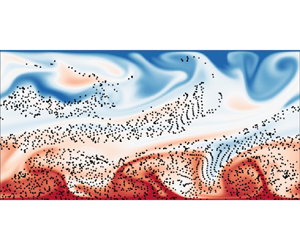
In figure 2, we show snapshots of temperature fields at various wall-shear Reynolds numbers $Re_w$ from 2-D simulations, and the corresponding movie can be viewed in supplementary movie 1. These snapshots are taken when half of the total particles remain suspended in the convection cell. The canonical RB convection (see figure 2a–c) consists of two large-scale rolls rotating in opposite directions. At lower $Re_w$ (see figure 2d–f), the horizontal wall-shear effects are weak, and the dominant flow patterns are similar to those in the canonical RB convection. As the wall shear increases, the large-scale rolls undergo horizontal expansion, eventually leading to a transition into the zonal flow state (see figure 2g–i). Zonal flows are primarily horizontal flows typically aligned with the rotation axis in rotating systems (Goluskin et al. Reference Goluskin, Johnston, Flierl and Spiegel2014; Zhang et al. Reference Zhang, Van Gils, Horn, Wedi, Zwirner, Ahlers, Ecke, Weiss, Bodenschatz and Shishkina2020; Lin & Jackson Reference Lin and Jackson2021) or along a specific direction in non-rotating systems (Wang et al. Reference Wang, Chong, Stevens, Verzicco and Lohse2020b; Winchester, Dallas & Howell Reference Winchester, Dallas and Howell2021; Jin et al. Reference Jin, Wu, Zhang, Liu and Zhou2022). These flows exhibit large-scale, coherent structures that can span the entire system and are often associated with banded structures in the flow field. Previous 2-D studies on zonal flow were primarily conducted in convection cells with free-slip boundaries, which do not exert shear stress to slow down the fluid, and the periodicity of the flow system allows for a horizontal mean flow (Goluskin et al. Reference Goluskin, Johnston, Flierl and Spiegel2014; Wang et al. Reference Wang, Chong, Stevens, Verzicco and Lohse2020b; Winchester et al. Reference Winchester, Dallas and Howell2021). In contrast, our work shows that moving boundaries induce a horizontal mean flow, forming the zonal flow. The overall trend in the 2-D flow pattern is similar to that in convection cells with rough shearing walls (Jin et al. Reference Jin, Wu, Zhang, Liu and Zhou2022).

Figure 2.

Typical instantaneous temperature fields (contours) and particle positions (black dots, sizes artificially increased for better flow visualization) from 2-D simulations at (a–c) $Re_w = 0$, (d–f) $Re_w = 2000$ and (g–i) $Re_w = 6000$, with $Ra=10^{8}$. Particle density is fixed as ${\rho _p}= 3000$ kg m$^{-3}$, with diameters of (a,d,g) ${d_p} = 5\,\mathrm {\mu }$m, (b,e,h) ${d_p}=20\,\mathrm {\mu }$m and (c, f,i) ${d_p} = 80\,\mathrm {\mu }$m. Corresponding Stokes numbers are (a) $St = 4.86 \times 10^{-4}$, (b) $St = 7.78 \times 10^{-3}$, (c) $St = 1.25 \times 10^{-1}$, (d) $St = 6.64 \times 10^{-4}$, (e) $St = 1.06 \times 10^{-2}$, ( f) $St = 1.70 \times 10^{-1}$, (g) $St = 3.93 \times 10^{-4}$, (h) $St = 6.29 \times 10^{-3}$ and (i) $St = 1.01 \times 10^{-1}$.

Regarding particle movement, the combined effects of particle diameter and particle density are reflected in the dimensionless Stokes number. For clarity of presentation, most results in this paper are shown at a fixed particle density but with varying particle diameters to present small, medium and large Stokes number cases. Particles with small $St$ (see figure 2a,d,g) are randomly distributed throughout the convection cell. These particles quickly adapt to changes in the surrounding flow, with little to no aggregation. For medium $St$ (see figure 2b,e,h), we observe a greater concentration of particles over upwelling areas, with downwelling regions displaying fewer particles. This counterintuitive observation aligns with our previous findings (Xu et al. Reference Xu, Tao, Shi and Xi2020) and independent research by Patočka et al. (Reference Patočka, Calzavarini and Tosi2020, Reference Patočka, Tosi and Calzavarini2022). The physical interpretation is that, for particles circulating within large-scale rolls in the convection cell, when they approach the bottom boundary beneath downwellings, they are likely to be carried by the fast-moving edges of the rolls toward regions beneath upwellings. In these upwelling regions, particles may enter areas with slower flow due to small-scale irregularities caused by new plume generation. These low-velocity regions increase the likelihood of particle sedimentation, leading to an accumulation of particles beneath the upwellings. In sheared convection cells, horizontal shear forces facilitate particle lateral dispersion, which is particularly apparent in figure 2(h). For large $St$ (see figure 2c, f,i), the inertia of the particles is dominant, causing them to settle and become nearly unresponsive to the carrier flow, similar to behaviour observed in quiescent fluid environments. As we will demonstrate later, even these large $St$ particles are slightly influenced by the turbulent flow.

In figure 3, we further show snapshots of the velocity component $v$ at the channel centre plane and particle positions from 3-D simulations, and the corresponding movie can be viewed in supplementary movie 2. In thermal convection, rising fluids are warmer and falling fluids are colder. At $Re_{w}=0$ and $Ra=10^{7}$, the flow structure resembles the canonical RB convection (Stevens et al. Reference Stevens, Blass, Zhu, Verzicco and Lohse2018). As $Re_{w}$ increases to 2000, the flow enters a transitional regime where the interaction between the imposed shear and buoyancy becomes significant. Large, elongated thermal plumes start to transform into thin, straight, elongated streaks aligned in the streamwise direction. Eventually, streamwise-oriented rolls are formed at $Re_{w}=4000$ (Pirozzoli et al. Reference Pirozzoli, Bernardini, Verzicco and Orlandi2017; Blass et al. Reference Blass, Zhu, Verzicco, Lohse and Stevens2020). To further elucidate the nature of these large-scale rolls, we present time-averaged streamlines coloured by the vertical velocity $v$, as shown in figure 4(a–c). At $Re_{w} = 0$, the averaged streamlines show a well-defined roll structure aligned in the spanwise direction. As $Re_{w}$ increases to 4000, the averaged streamlines transition to an organized pattern aligned with the streamwise direction. Additionally, we measure the velocity orientation $\theta$, defined as the angle between the projection of the velocity vector onto the $x$–$z$ plane and the positive $x$-axis. We calculate the probability density functions (p.d.f.s) of $\theta$ for fluid nodes in the region $0.1H \le y \le 0.9H$, and present their time evolution in figure 4(d–f). At $Re_{w}=0$, the p.d.f.s indicate high probability values consistently around $0^\circ$ and $180^\circ$, suggesting that the roll axes are predominantly aligned in the spanwise direction, without exhibiting complex motions as seen in an RB cell with a larger length-to-width aspect ratio (Vogt et al. Reference Vogt, Horn, Grannan and Aurnou2018; Li et al. Reference Li, Chen, Xu and Xi2022; Teimurazov et al. Reference Teimurazov, Singh, Su, Eckert, Shishkina and Vogt2023). At $Re_{w}=4000$, the p.d.f.s shift to show high probability values around ${\pm }90^\circ$, indicating that the roll axes are consistently aligned in the streamwise direction.

Figure 3.

Typical instantaneous slice of velocity component $v$ at the channel centre plane (contours) and particle positions (black dots, sizes artificially increased for better flow visualization, here 0.8 % of suspended particles are shown for clarity) from 3-D simulations at (a–c) $Re_w = 0$, (d–f) $Re_w = 2000$ and (g–i) ${Re_w = 4000}$, with $Ra=10^{7}$. Particle density is fixed as ${\rho _p}= 3000$ kg m$^{-3}$, with diameters of (a,d,g) ${d_p} = 5\,\mathrm {\mu }$m, (b,e,h) ${d_p}=20\,\mathrm {\mu }$m and (c, f,i) ${d_p} = 80\,\mathrm {\mu }$m. Corresponding Stokes numbers are (a) $St = 7.05 \times 10^{-4}$, (b) $St = 1.13 \times 10^{-2}$, (c) $St = 1.80 \times 10^{-1}$, (d) $St = 7.70 \times 10^{-4}$, (e) $St = 1.23 \times 10^{-2}$, ( f) $St = 1.97 \times 10^{-1}$, (g) $St = 8.83 \times 10^{-4}$, (h) $St = 1.41 \times 10^{-2}$ and (i) $St = 2.26 \times 10^{-1}$.

Figure 4.

(a–c) Time-averaged streamlines coloured by the vertical velocity $v$, (d–f) time evolution of the p.d.f.s of the instantaneous velocity orientation $\theta$ at (a,d) $Re_w = 0$, (b,e) $Re_w = 2000$ and (c, f) $Re_w = 4000$, with $Ra=10^{7}$.

We then examine the global response parameters of the Nusselt number ($Nu$) and Reynolds number ($Re$) on the control parameter $Re_w$ in the 2-D flow system. Here, the heat transfer efficiency is calculated as $Nu = 1 + \sqrt {PrRa} {\langle v^*T^*\rangle _{V,t}}$, and the global flow strength of the convection is calculated as $Re = \sqrt {{{\langle \|\boldsymbol {u} \|^{2} \rangle }_{V,t}}} H/\nu _f$. Moreover, we consider the lateral and vertical components of $Re$, respectively, as $Re_{x} = \sqrt {{{\langle {u^2}\rangle }_{V,t}}} H/\nu _f$, $Re_{y} = \sqrt {{{\langle {v^2}\rangle }_{V,t}}} H/\nu _f$. Both $Nu$ and $Re$ exhibit sharp changes and abrupt transitions at $Re_w \simeq 1500$ with $Ra=10^7$ (see figure 5a,d), at $Re_w \simeq 5000$ with $Ra=10^8$ (see figure 5b,e), suggesting a threshold for the competition between wall shear and buoyancy that leads to changes in the flow state from LSCs to zonal flows in 2-D simulations. The heat transport behaviour in wall-sheared thermal turbulence is governed by the interaction between the buoyancy-driven LSC and the shear introduced by the moving walls. At higher wall shear, strong wall instabilities disrupt the large-scale rolls, which are crucial for carrying thermal energy away from the wall and efficiently transporting heat. When these large-scale structures are disrupted, small-scale turbulent motions become more prevalent, and the convective motions near the wall increase. However, these motions become more localized and less effective in transporting heat across larger vertical distances, thus decreasing the overall efficiency of heat transport. Regarding the velocity fields, LSCs exhibit both significant vertical and horizontal velocity components, while zonal flows in two dimensions show strong horizontal velocities with a lower vertical component. At a fixed Rayleigh number, when the wall shear becomes sufficiently strong, the flow transitions to laminar Couette flow, causing the vertical flow velocity component to become nearly zero. For a Rayleigh number of $10^{7}$, this transition occurs approximately at $Re_{w} \simeq 2000$ (see figure 5d); for a Rayleigh number of $10^{8}$, the transition happens at around $Re_{w} \simeq 8000$ (see figure 5e). At an even higher Rayleigh number of $10^{9}$, based on the results of Jin et al. (Reference Jin, Wu, Zhang, Liu and Zhou2022) and Xu et al. (Reference Xu, Xu and Xi2023), we speculate that the transitions to laminar Couette flow occurs at a much larger $Re_{w}$, beyond the parameter range explored in the present work.

Figure 5.

(a–c) Nusselt number and (d–f) Reynolds number as a function of $Re_w$: (a,d) with $Ra=10^{7}$, (b,e) with $Ra=10^{8}$, (c, f) with $Ra=10^{9}$.

We quantitatively describe the influence of wall shear on particle motion by analysing the p.d.f.s of their velocity components ($u_p$ and $v_p$), as shown in figure 6. For particles with small and medium $St$ (see figure 6a,b), the p.d.f.s of $u_p$ are characterized by a single peak centred around zero, exhibiting symmetry for $Re_w \lesssim 5000$, suggesting a substantial likelihood of particles circulating within the LSC of convective flows. As $Re_w$ increases to 6000, the p.d.f.s of $u_p$ change to a bimodal distribution with two peaks off zero value, which can be attributed to the horizontal drift of particles caused by the wall shear. In addition, with increasing $St$, the peak corresponding to the negative $u_p$ exceeds that of the positive, suggesting an increased likelihood for particle suspension in the lower domain of the cell due to sedimentation (note the bottom wall is moving in the negative $x$-direction). For large $St$ (see figure 6c), we can deduce that these particles are still minorly influenced by the turbulent flow because they exhibit horizontal motions with finite positive or negative $u_p$. Regarding the p.d.f.s of $v_p$, for small and medium $St$ (see figure 6d,e), their shapes are much narrower at $Re_w = 6000$ compared with those at lower $Re_w$, indicating attenuated vertical motions in the zonal flow. This trend becomes more pronounced for large $St$ (see figure 6f), where $v_p$ values are predominantly negative. This implies vertical updrafts are insufficient to counter the gravitational settling, preventing these particles from rising with the flow currents.

Figure 6.

The p.d.f.s of the particle velocity component (a–c) in the horizontal direction ($u_p$), and (d–f) in the vertical direction ($v_p$) with $Ra=10^{8}$. Particle density is fixed as ${\rho _p}= 3000$ kg m$^{-3}$, with diameters of (a,d) ${d_p} = 5\,\mathrm {\mu }$m, (b,e) ${d_p}=20\,\mathrm {\mu }$m and (c, f) ${d_p} = 80\,\mathrm {\mu }$m.

We examine the p.d.f.s of the particle Reynolds number $Re_{p} = {d_p}|{{\boldsymbol {u}}_f} - {{\boldsymbol {u}}_p}|/{\nu _f}$, as shown in figure 7. We can see from figure 7(a,b) that, for particles with small $St$, $Re_p$ is generally less than $10^{-3}$; for medium $St$, $Re_p$ is generally less than $10^{-1}$. In the presence of a pronounced LSC within the flow, the p.d.f.s of $Re_p$ manifest dual peaks, corresponding to the particles ascending or descending with the LSC. As wall shear increases, the $Re_p$ will also increase and exhibit enhanced intermittency. However, when $Re_w$ further increases up to 6000, $Re_p$ decreases and the p.d.f.s of $Re_p$ change from a bimodal to unimodal distribution. This shift is attributed to the decreased vertical velocity component $v_p$ of the particles within the convective flow, as evidenced by figure 6(d–f). For large $St$, $Re_p$ is as large as $Re_p\sim O(1)$ and spans a more extensive range, as shown in figure 7(c), which emphasizes the necessity of incorporating a drag correction factor $f(Re_{p})$ into the drag force calculations. We further plot the p.d.f.s of normalized particle Reynolds number $(Re_{p} - {\mu _{Re_{p}}})/{\sigma _{Re_{p}}}$, as shown in figure 7(d–f). For particles with small $St$ (see figure 7d), the p.d.f.s of $Re_p$ are close to the Gaussian distribution (denoted by the dashed line in the figure). However, with an increase in $Re_w$, the deviations in the tails of the p.d.f.s. become more pronounced, indicating more intermittency events due to the influence of wall shear. For medium $St$ (see figure 7e), the p.d.f.s generally follow the Gaussian distribution, although there appear to be deviations with heavier tails, which implies there are more instances of $Re_p$ values deviating from the mean. For large $St$ (see figure 7f), the p.d.f.s of $Re_p$ are distinctly different from a Gaussian distribution, indicating a distinct distribution pattern where particle motion is nearly unaffected by the turbulence.

Figure 7.

(a–c) The p.d.f.s of particle Reynolds number $Re_p$ and (d–f) the p.d.f.s of normalized particle Reynolds number $(Re_{p} - {\mu _{Re_{p}}})/{\sigma _{Re_{p}}}$ with $Ra=10^{8}$. Particle density is fixed as ${\rho _p}= 3000$ kg m$^{-3}$, with diameters of (a,d) ${d_p} = 5\,\mathrm {\mu }$m, (b,e) ${d_p}=20\,\mathrm {\mu }$m and (c, f) ${d_p} = 80\,\mathrm {\mu }$m. Dashed lines in (d–f) represent the Gaussian distribution.

Previous studies have shown that, even in homogeneous isotropic turbulence, the particles may not distribute homogeneously but exhibit clustering behaviour (Wang & Maxey Reference Wang and Maxey1993; Bosse, Kleiser & Meiburg Reference Bosse, Kleiser and Meiburg2006; Calzavarini et al. Reference Calzavarini, Kerscher, Lohse and Toschi2008). To identify the clustering behaviour of particles during their transport in the wall-sheared convection cell, we employ a quantitative analysis using Voronoï diagrams (Monchaux, Bourgoin & Cartellier Reference Monchaux, Bourgoin and Cartellier2010, Reference Monchaux, Bourgoin and Cartellier2012). A Voronoï cell is defined as a collection of points closer to its corresponding particle than to any other; thus, the area (or volume) of a Voronoï cell inversely correlates with local particle concentration. In figure 8, we show Voronoï diagrams for the particle distribution, corresponding to the instantaneous state presented in figure 2. For particles with small $St$ (see figure 8a,d,g), Voronoï cells are of similar size and relatively evenly distributed in space, indicating a low degree of aggregation. For medium $St$ (see figure 8b,e,h), the areas of their Voronoï polygon exhibit much higher variability, indicating an increased level of spatial inhomogeneity. For large $St$ (see figure 8c, f,i), large voids are formed at the upper part of the convection cell, containing few to no particles. This is because most particles settle down and do not circulate in the cell, as revealed by the predominantly negative $v_p$ velocity components shown in figure 6( f).

Figure 8.

Typical instantaneous Voronoï diagrams for particles at (a–c) $Re_w = 0$, (d–f) $Re_w = 2000$, (g–i) $Re_w = 6000$ with $Ra=10^{8}$. Particle density is fixed as ${\rho _p}= 3000$ kg m$^{-3}$, with diameters of (a,d,g) ${d_p} = 5\,\mathrm {\mu }$m, (b,e,h) ${d_p}=20\,\mathrm {\mu }$m and (c, f,i) ${d_p} = 80\,\mathrm {\mu }$m.

We then analyse the statistical distribution of the Voronoï cell area $A$. Figure 9 shows the p.d.f.s of the normalized Voronoï cell area $A/\langle A \rangle$, corresponding to the instantaneous state presented in figure 8. Here, $\langle A \rangle$ represents the mean value of $A$ at the current moment. For particles with small $St$ (see figure 9a), the Voronoï cells are randomly distributed throughout the flow field, and the distribution of their areas satisfies the $\varGamma$ distribution (Ferenc & Néda Reference Ferenc and Néda2007; Tagawa et al. Reference Tagawa, Mercado, Prakash, Calzavarini, Sun and Lohse2012)

(3.1)\begin{equation} f_d(m) = \frac{[(3d + 1)/2]^{(3d + 1)/2}}{\varGamma [(3d + 1)/2]} m^{(3d - 1)/2} \exp \left( - \frac{3d + 1}{2} m\right),\quad m = \frac{A}{\langle A \rangle}, \end{equation}

where $d = 2$ denotes the analysis in two dimensions. For medium $St$ (see figure 9b), the p.d.f.s have a peak near unity, yet exhibit pronounced tails indicative of larger Voronoï cell areas, deviating from the $\varGamma$ distribution. This deviation from the $\varGamma$ distribution signals a departure from randomness, indicative of local preferential concentration. For large $St$ (see figure 9c), the p.d.f.s exhibit more pronounced tails towards larger Voronoï cell areas, indicating intensified void formation.

Figure 9.

(a–c) The p.d.f.s of the normalized Voronoï cell area $A/\langle A \rangle$ corresponding to the instantaneous state presented in figure 8, and (d–f) time evolution of the standard deviation of the normalized Voronoï cell area. Panels show (a,d) ${d_p} = 5\,\mathrm {\mu }$m, (b,e) ${d_p}=20\,\mathrm {\mu }$m and (c, f) ${d_p} = 80\,\mathrm {\mu }$m.

Figure 9(d–f) further shows the time evolution of the standard deviation $\sigma$ of the normalized Voronoï cell area, serving as an indicator of spatial inhomogeneity. Due to particle deposition on the wall and constantly reducing particle numbers, the particles statistics cannot reach a statistically stationary state. Here, we only plot the time series from the initial state to the time at which half of the total particles remain suspended in the convection cell. For particles with small $St$ (see figure 9d), the standard deviation is the lowest, approaching the theoretical expectation for the $\varGamma$ distribution (i.e. $\sigma = 0.53$, denoted by the dash-dotted line). For medium $St$ (see figure 9e), the greatest clustering is observed as the standard deviation of their Voronoï area significantly exceeds 0.53. For large $St$ (see figure 9f), the clustering also occurs; however, the influence of variations in wall-shear strength $Re_w$ appears to be negligible in contrast to those with medium $St$.

Based on the above analysis, we arrive at the following mathematical model for the spatial distribution of particle concentration. We denote the initial concentration of particles as ${n_0} = {N_0}/(LHW)$, where $N_{0}$ is the initial number of particles laden in the fluid. We define the instantaneous particle line density averaged over a horizontal cross-section as $n(\tau,y) = N(\tau,y)/(LW)$ at a given time $\tau$ and height $y$, where $N(\tau,y)$ is the instantaneous particle number at time $\tau$ and height $y$. We also define the time-averaged local particle concentration over a horizontal cross-section and along the cell height as $\langle n(y) \rangle _{t}$, where the average $\langle {\cdot } \rangle _{t}$ is calculated over time $t$. In transient processes, the particle concentration changes over time, and the time-averaged concentration represents the overall behaviour of the particles during a specified time interval, which is crucial for understanding the long-term behaviour of the system, even when the process is not in a steady state.

For particles with small $St$, they are randomly distributed throughout the convection cell, and they exhibit an exponential decay rate as ${N(\tau )} = N_{0}\exp [ { -\tau }/( {H/{v_t}} ) ]$ (Martin & Nokes Reference Martin and Nokes1989), with $N(\tau )$ being the number of particles that remain laden in the convection cell at time $\tau$. Following the assumption of Martin & Nokes (Reference Martin and Nokes1989), turbulent convection ensures that particles are mixed homogeneously across the flow, which leads to $N(\tau,y)=N(\tau )/H$, and particle concentration is uniform across the horizontal plane of the fluid. Thus, at a given time $\tau$ and height $y$, the instantaneous particle line density $n(\tau,y)$ is

(3.2)\begin{equation} n(\tau,y) = \frac{N(\tau,y)}{LW} = \frac{N(\tau)}{LHW} = \frac{N_0 \exp \left( - \dfrac{\tau}{H/v_t} \right)}{LHW} = n_0 \exp \left( - \frac{\tau}{H/v_t} \right). \end{equation}

Then, the horizontal- and time-averaged local particle concentration, which represents the number density of particles suspended in the convection cell over a given time period and horizontal cross-section, for small $St$, is

(3.3)\begin{equation} \frac{\langle n(y)\rangle_t}{n_0}= \frac{\displaystyle\left( \int_0^t n(\tau, y)\,{\rm d}\tau \right) / t}{n_0} ={-} \frac{H}{v_t t} \left[ \exp \left( - \frac{t}{H / v_t} \right) - 1 \right]. \end{equation}

In the above, $\langle n( y ) \rangle _{t}$ is further normalized by initial concentration $n_0$.

For large $St$, sedimentation occurs almost independently of the carrier flow, analogous to settling behaviour of particles in quiescent fluid environments. Thus, we can ignore their lateral motion and simply assume they settle at a constant speed of terminal velocity $v_t$. From the initial state of uniform distribution, after a duration of $\tau$, the particle ensemble settles a vertical distance of $v_t \tau$. Thus, the instantaneous particle line density $n(\tau, y)$ is

(3.4)\begin{equation} n(\tau, y) = \begin{cases} 0, & H - v_t \tau < y \le H \\ n_0, & y \le H - v_t \tau . \end{cases} \end{equation}

We consider at the time $\tilde {t} \in [ {0,t} ]$ the instantaneous local particle concentration $n(\tilde {t}, y)$ that decreases from ${n_0}$ to 0 across a height interval $\tilde y$, where $\tilde y \in [ {H - {v_t}\tilde {t},H} ]$, resulting in $H - {v_t}\tilde t = \tilde y$. Thus, the horizontal- and time-averaged local particle concentration (further normalized by ${n_0}$), for large $St$, is

(3.5)\begin{equation} \frac{\langle n(y)\rangle_t}{n_0}= \frac{\displaystyle\left(\int_0^t n(\tau, y)\,{\rm d}\tau \right) / t}{n_0} = \begin{cases} \dfrac{\displaystyle\left(\int_0^{\tilde{t}} n_0 \, {\rm d}\tau \right) / t}{n_0} + \dfrac{\displaystyle\left(\int_{\tilde{t}}^t 0 \, {\rm d}\tau \right) / t}{n_0}, & H - v_t t \le y \le H \\ \dfrac{\displaystyle\left(\int_0^t n_0 \, {\rm d}\tau \right) / t}{n_0}, & y \le H - v_t t . \end{cases} \end{equation}

The above equation can be further simplified to

(3.6)\begin{equation} \frac{\langle n(y)\rangle_t}{n_0} = \begin{cases} \dfrac{H - y}{v_t t}, & H - v_t t \le y \le H \\ 1, & y \le H - v_t t . \end{cases} \end{equation}

We choose the time-average $\langle {\cdot } \rangle _{t_{1/2}}$ from the initial state up to the state when half of the total particles deposit on the wall (a duration referred to as half-life time $t_{1/2}$ from now on). For particles with small $St$, they exhibit an exponential deposition rate (Martin & Nokes Reference Martin and Nokes1989). The half-life time can be obtained by setting $N_s/N_0 = 1 - \exp [ { - t_{1/2}/( {H/{v_t}} )} ]=1/2$, which further gives $t_{1/2} = ( {H\ln 2} )/{v_t}$. Here, $N_{s}$ is the number of particles that have settled and deposited on the wall. Substituting this time duration into (3.3), we derive the horizontal- and time-averaged local particle concentration for small $St$ as

(3.7)\begin{equation} \frac{\langle n(y)\rangle_{t_{1/2}}}{n_0} = \frac{1}{2 \ln 2} . \end{equation}

For large $St$, the deposition rate on the wall follows a linear law as derived from Stokes’ law. The half-life time can be obtained by setting $N_s/N_0 = t_{1/2}/(H/v_{t})=1/2$, which further gives $t_{1/2} = 0.5H/{v_t}$. Substituting this into (3.6), we derive the horizontal- and time-averaged local particle concentration for large $St$ as

(3.8)\begin{equation} \frac{\langle n(y) \rangle_{t_{1/2}}}{n_0} =\begin{cases} 2\left( 1 - \dfrac{y}{H} \right), & 0.5H \le y \le H \\ 1, & y \le 0.5H . \end{cases} \end{equation}

In figure 10, we compare the theoretical estimations of ${\langle {n( y )} \rangle _{t_{1/2}}}/{n_0}$, namely (3.7) and (3.8), with both 2-D and 3-D simulation results. For particles with small $St$ (see figure 10a,d), the local particle concentration generally agrees with the theoretical predictions except for the discrepancy at $y > 0.8 H$. This discrepancy may be attributed to the finite $St$ effect (i.e. a small but not non-zero $St$), which results in a reduced particle presence in the upper boundary layer. At $Re_w = 6000$ in the 2-D simulations, the flow transitions from the LSC to zonal flow, thus the assumption of a spatially uniform particle concentration proposed by Martin & Nokes (Reference Martin and Nokes1989) may no longer be valid, leading to significant deviation from (3.7). Specifically, when the LSC transitions to a zonal flow state, the updrafts are significantly weakened. This weakening results in fewer particles drifting upwards and more particles settling down, leading to a higher particle concentration at the bottom of the zonal flow compared with the LSC state. For medium $St$ (see figure 10b,e), the absence of a corresponding model precludes a direct comparison; however, we provide a qualitative description of particle concentration. When the LSC is present, the local particle concentration appears to be consistent in the bulk region, but exhibits an increase with increasing $Re_w$ in the bottom boundary layer, implying that wall shear accelerates particle sedimentation. At $Re_w = 6000$ in the 2-D simulations, the changes in flow states lead to distinctly different profiles for the local particle concentration compared with those at lower $Re_w$. For large $St$ (see figure 10c, f), the local particle concentration generally agrees with the theoretical prediction (3.8) across all $Re_w$, highlighting again that the particles’ motion is nearly not affected by the turbulent flows of the carrier fluid (i.e. either LSC or zonal flow state). When the wall shear becomes sufficiently strong, the vertical flow velocity component weakens significantly. Since the settling velocity of particles is strongly influenced by the vertical flow velocity component, the settling velocity of particles then approaches that in a stationary flow field (i.e. the terminal velocity $v_{t}$). This explains why the concentration profile for $Re_{w} = 6000$ in figure 10(b) is similar to those in figure 10(c) for the 2-D simulation.

Figure 10.

Vertical profiles of the horizontal- and time-averaged local particle concentration obtained from (a–c) the 2-D simulation with $Ra=10^{8}$ and (d–f) the 3-D simulation with $Ra=10^{7}$. Particle density is fixed as ${\rho _p}= 3000$ kg m$^{-3}$, with diameters of (a,d) ${d_p} = 5\,\mathrm {\mu }$m, (b,e) ${d_p}=20\,\mathrm {\mu }$m and (c, f) ${d_p} = 80\,\mathrm {\mu }$m. The pink solid line in (a,d) corresponds to (3.7), and the blue solid line in (c, f) corresponds to (3.8).

3.2. Particle deposition on the wall

To quantify the particle deposition behaviour, we first examine the p.d.f.s of their deposition locations along the bottom wall, as shown in figure 11. In our simulations, the particles adhere to the wall upon contact, and we then mark them as deposited and record the contact position as the deposition location. For particles with small $St$ (see figure 11a), the deposition locations are uniformly distributed along the bottom wall, aligning with the assumption of a spatially uniform particle concentration. For medium $St$ (see figure 11b), there is pronounced aggregation behaviour for deposition positions along the bottom wall. With the increase of $Re_w$, the degree of aggregation weakens, possibly because wall shear causes the boundary layers to move horizontally, thereby dispersing the particles to deposit more evenly along the bottom wall. We also observed a correlation between the regions of particle accumulation on the bottom wall and the rising of hot plumes (compared with figure 2), as revealed in our previous findings (Xu et al. Reference Xu, Tao, Shi and Xi2020) and independent research by Patočka et al. (Reference Patočka, Calzavarini and Tosi2020, Reference Patočka, Tosi and Calzavarini2022). The accumulation of heavy particles beneath upwellings seems somewhat counterintuitive, as one might expect these particles to accumulate primarily beneath significant downwellings. For large $St$ (see figure 11c), the uniformity of the deposition pattern is restored, mainly attributed to the reduced influence of the carrier flow on these particles, resulting in an initial uniform distribution less affected by the carrier flow, unlike their low $St$ counterparts.

Figure 11.

The p.d.f.s of particle deposition locations along the bottom wall with $Ra=10^{8}$. Particle density is fixed as ${\rho _p}= 3000$ kg m$^{-3}$, with diameters of (a) ${d_p} = 5\,\mathrm {\mu }$m, (b) ${d_p}=20\,\mathrm {\mu }$m and (c) ${d_p} = 80\,\mathrm {\mu }$m.

We quantify the deposition ratio as the ratio of settled particles $N_s$ to the initial total number $N_0$, and plot the settling curve $N_s/N_0$ from 2-D simulations as shown in figure 12. For particles with small $St$, Martin & Nokes (Reference Martin and Nokes1989) predicted an exponential deposition rate ${N_s}/{N_0} = 1 - \exp [ { - t/({H/{v_t}} )} ]$, and our simulation results confirmed the theoretical prediction at $Re_w \le 4000$ (see figure 12a,d). However, departure from the expected exponential rate was observed at $Re_w = 6000$ (see figure 12g), where the LSC was absent and the flow state transitioned to zonal flow. The main reason is that Martin & Nokes (Reference Martin and Nokes1989) assumed convective velocities were negligible at the bottom boundary layer of the canonical convection cell; in contrast, in the strong wall-sheared convection, horizontal shear velocities persist in the boundary layer, resulting in the failure of the assumption and the deviation in the settling curve. For large $St$, a simple model assumes that these particles, being less influenced by the carrier flow, follow a linear deposition rate $N_s/N_0 = t/( {H/{v_t}} )$. We can see from figure 12(c, f,i) that our simulation results agree with the linear rate at $t < H/{v_t}$, yet deviations are observed at the tails of the settling curve, indicating that a longer time than $H/{v_t}$ is required for all the particles to eventually deposit on the wall. A possible explanation is that the carrier flow still has a subtle influence on particles with large $St$ (yet not infinitely large), and this influence becomes increasingly pronounced as time progresses. In figure 13, we further plot the settling curve $N_{s}/N_{0}$ from 3-D simulations. Overall, the 3-D simulation results reinforce the findings from the 2-D simulations that small $St$ particles settle with an exponential deposition ratio and large $St$ particles settle with a linear deposition ratio.

Figure 12.

Settling curves from 2-D simulations with $Ra=10^{8}$ at (a–c) $Re_w = 0$, (d–f) $Re_w = 2000$ and (g–i) $Re_w = 6000$. Particle density is fixed as ${\rho _p}= 3000$ kg m$^{-3}$, with diameters of (a,d,g) ${d_p} = 5\,\mathrm {\mu }$m, (b,e,h) ${d_p}=20\,\mathrm {\mu }$m and (c, f,i) ${d_p} = 80\,\mathrm {\mu }$m. The insets in (a,d,g) magnify differences between our new model and the exponential law, and insets in (c, f,i) magnify differences between our new model and the linear law.

Figure 13.

Settling curves from 3-D simulations with $Ra=10^{7}$ at (a–c) $Re_w = 0$, (d–f) $Re_w = 2000$ and (g–i) $Re_w = 4000$. Particle density is fixed as ${\rho _p}= 3000$ kg m$^{-3}$, with diameters of (a,d,g) ${d_p} = 5\,\mathrm {\mu }$m, (b,e,h) ${d_p}=20\,\mathrm {\mu }$m and (c, f,i) ${d_p} = 80\,\mathrm {\mu }$m. The insets in (a,d,g) magnify differences between our new model and the exponential law, and insets in (c, f,i) magnify differences between our new model and the linear law.

Despite existing simple models predicting particle deposition rates for small and large $St$, challenges arise for medium $St$ due to the complex particle–turbulence interactions. Examining the settling curves obtained from simulation, we develop the following model that comprises a linear settling stage succeeded by a nonlinear settling stage. We denote by $t_{s}$ the transient time from the linear to the nonlinear stage. At the early settling stage, particles initially released in the lower domain and in the downwelling areas tend to settle. To illustrate this, we conducted an a posteriori examination and marked the initial positions of particles that settle during the linear stage, as shown in figure 14(a–c). The particle drift equation (Patočka et al. Reference Patočka, Tosi and Calzavarini2022) gives $\boldsymbol {u}_{p}=\boldsymbol {u}_{f}+\boldsymbol {v}_{t}$ in the limit of $St \ll 1$, where $\boldsymbol {v}_{t}$ is the particle Stokes velocity. This equation indicates that particles subjected to updrafts settle at a speed of ${v_t} - {v_f}$, while those in downdrafts settle at ${v_t} + {v_f}$. Here, ${v_f}$ denotes the vertical flow speed at the particle's position. At this stage, the settling particles decrease height almost monotonically, without recirculating in the convection cell, as shown in figure 15(a–c). Assuming the same proportion of settling particles affected by the updraft in the lower domain and downdraft in the downwelling areas, then the numbers of $N_{up}$ and $N_{down}$ during $t \le {t_s}$ are

(3.9a,b)\begin{equation} N_{up} = \frac{N_0}{2} \frac{(v_t - v_f) tLW}{HLW},\quad N_{down} = \frac{N_0}{2} \frac{(v_t + v_f) tLW}{HLW}, \end{equation}

thus, at this settling stage, the deposition ratio (i.e. the fraction of particles that have deposited on the wall relative to the initial number of particles laden in the flow system) is

(3.10)\begin{equation} \frac{N_s}{N_0} = \frac{N_{up} + N_{down}}{N_0} = \frac{t}{H / v_t} . \end{equation}

The above relation indicates that the deposition ratio linearly increases with time, which is why we name it the linear stage.

Figure 14.

An a posteriori examination of the initial positions (black dots) for particles that have settled (a–c) during the linear stage and (d–f) during the nonlinear stage, alongside the corresponding instantaneous temperature fields (contours) at (a,d) $Re_w = 0$, (b,e) $Re_w = 2000$ and (c, f) $Re_w = 6000$, with $Ra=10^{8}$. Particle density is fixed as ${\rho _p}= 3000$ kg m$^{-3}$ and diameter is fixed as ${d_p}=20\,\mathrm {\mu }$m. Note this figure does not represent a ‘real’ instantaneous particle distribution within the convection cell.

Figure 15.

Example particle trajectories for those settled (a–c) during the linear stage and (d–f) during the nonlinear stage at (a,d) $Re_w = 0$, (b,e) $Re_w = 2000$ and (c, f) $Re_w = 6000$, with $Ra=10^{8}$. Particle density is fixed as ${\rho _p}= 3000$ kg m$^{-3}$ and diameter is fixed as ${d_p}=20\,\mathrm {\mu }$m. The trajectories are coloured according to the normalized suspension time of the particles. The blue circle marks the initial position and the red star marks the deposition position.

At the later nonlinear settling stage, particles initially released in the roll centre and upwelling areas tend to settle, as illustrated in figure 14(d–f). The particles circulate within the large-scale roll and may escape the circulation due to small-scale irregularities produced by the emergence of new plumes (Patočka et al. Reference Patočka, Calzavarini and Tosi2020). With the increase of wall shear, the lateral motion increases, making the particles more likely to escape the circulation, as shown in figure 15(d–f). Inspired by the stochastic model proposed by Denzel, Bragg & Richter (Reference Denzel, Bragg and Richter2023), we denote the time duration for a particle to complete the circulation as $t_c$ and the escape probability from the circulation as $\lambda _f$. The time decay rate of particle number $N$ in the convection cell is

(3.11)\begin{equation} {\rm d} N ={-} \lambda_f \frac{{\rm d} t}{t_c} N(t) \Rightarrow N(t) = C_0 \exp \left( - \frac{\lambda_f}{t_c} t \right), \end{equation}

thus, at the nonlinear settling stage, the deposition ratio is

(3.12)\begin{equation} \frac{N_s}{N_0} = \frac{N_0 - N}{N_0} = 1 - C_1 \exp \left( - \frac{\lambda_f}{t_c} t \right) = 1 - C_1 \exp \left( - \frac{C_2}{H / v_t} t \right), \end{equation}

where $C_1 = C_0/N_0$ and $C_2 = H\lambda _f/(v_t t_c)$ involves a combination of unknowns $t_c$ and $\lambda _f$.

In short, we propose a new model that describes the settling process via an early linear stage and a later nonlinear stage, written as

(3.13)\begin{equation} \frac{N_s}{N_0} = \begin{cases} \dfrac{t}{H / v_t}, & t \le t_s \\ 1 - C_1 \exp \left( - \dfrac{C_2}{H / v_t} t \right), & t \ge t_s. \end{cases} \end{equation}

Under the assumption of a smooth settling curve, namely $N_{s}/N_{0}$ is continuously changing at $t_{s}$, we then have ${C_1} = [ {1 - {t_s}/(H/{v_t})} ]/\exp [ { - {C_2}{t_s}/( {H/{v_t}} )} ]$. The determination of $t_s$ and $C_2$, essential for model closure, will be achieved by least square fitting of the settling curves.

Previously, in figures 12 and 13, we compared results from this newly developed model with 2-D and 3-D simulation results, respectively. Good agreement was observed for convective flows across various $Re_w$ and particles with a wide range of $St$. Although our original motivation was to propose a model to predict particle deposition rates for medium $St$, the simulation results indicate that our model is applicable for small and large $St$ as well. In figures 12 and 13, we also plot the predictions from the Patočka et al. model (denoted as the $f$ distribution) (Patočka et al. Reference Patočka, Calzavarini and Tosi2020, Reference Patočka, Tosi and Calzavarini2022). The key idea of the $f$ distribution is to describe particle settling as $\textrm {d} N/\textrm {d} t=-N(t)/(fH/v_{t})$, leading to a settling curve determined by $N(t)/N_{0}=\exp [-v_{t}t/(Hf)]$. We observe a clear departure in the settling curve, mainly because their model adopts a unified exponential solution to describe the settling process, whereas DNS results indicate a linear regime in the settling curves (see also in Patočka et al. (Reference Patočka, Calzavarini and Tosi2020), figure 3). As acknowledged by Patočka et al. (Reference Patočka, Calzavarini and Tosi2020), the imperfect fit of the observed settling curves is due to the fact that $f$ should be a function of time rather than remaining constant. This time dependency of $f$ results in a misfit between the $f$ distribution and the observed settling curves, with the largest error occurring for particles with a medium Stokes number. Nevertheless, Patočka et al.'s model is still useful for estimating the characteristic time of sedimentation, as discussed later in this paper.

For our new model to be fully closed and predictive, we still need to provide accurate modelling of the parameters $t_s$ and $C_2$. In figure 16, we plot $t_s$ and $C_2$ as a function of $St_{f}$ for various $Re_w$ in the 2-D cell with $Ra=10^{8}$. Here, we adopt $St_f$ rather than $St_K$ as the input parameter because $St_f$ is simpler to determine from the flow parameters, making it more convenient for modelling. In Appendix B we further examine the Rayleigh number dependence of such a relationship with $Ra=10^{7}$ and $10^{9}$. We can see from figure 16(a), for medium $St_{f}$ in the range of $10^{-3} \le St_{f} \le 10^{-2}$, the parameter $t_s$ can be empirically estimated as

(3.14)\begin{equation} \frac{t_s}{H/v_t} = \begin{cases} 0.47 \log_{10}(St_{f}) + 1.70, & \text{if large-scale roll} \\ 0.32 \log_{10}(St_{f}) + 1.50, & \text{if zonal flow} . \end{cases} \end{equation}

This implies that $t_s$ is minorly influenced by $Re_w$ when the convective flow state remains unchanged (either in the LSC or zonal flow state). Practically, to empirically estimate $t_{s}$ using the above equation, we should first determine the flow states, then $t_{s}$ can be empirically expressed as a function of the Stokes number. This $t_{s}$ value is essentially an ensemble-averaged value for all the particles. As for the parameter $C_2$ (see figure 16b), although its original definition is just a combination of unknowns of $t_c$ and $\lambda _f$, for the convenience of mathematical calculation, in the following, we will reveal the physical meaning of this parameter $C_2$.

Figure 16.

Dependence of the parameters (a) $t_s$ and (b) $C_2$ on the Stokes number $St$ for various wall-shear Reynolds numbers $Re_w$, with $Ra=10^{8}$. The black solid and dashed lines in (a) represent the empirical relations (3.14).

According to the particle mass conservation equation (Martin & Nokes Reference Martin and Nokes1989; Patočka et al. Reference Patočka, Tosi and Calzavarini2022), the particle deposition rate $\textrm {d} N/\textrm {d} t$ is equal to the decrease of particle flux $A_0 v_t n_{bnd}$ at the lower boundary, namely, $\textrm {d} N/\textrm {d} t = - A_0 v_t n_{bnd}$. Here, $A_0$ is the area (or length in the 2-D case) of the bottom boundary, and $n_{bnd}$ is the mean particle number concentration near the lower boundary. Because the particle deposition rate is

(3.15)\begin{equation} \frac{{\rm d} N}{{\rm d} t} =\begin{cases} - v_t L \dfrac{N_0}{LHW}, & t < t_s \\ - v_t L C_2 \dfrac{N(t)}{LHW}, & t \ge t_s \end{cases}=\begin{cases} - v_t L n_0, & t \le t_s \\ - v_t L C_2 \langle n(t) \rangle_{V}, & t \ge t_s \end{cases}, \end{equation}

where $\langle {n( t )} \rangle _{V} = N(t)/(LHW)$ is the instantaneous volume-averaged concentration, then we have

(3.16)\begin{equation} n_{bnd} = \begin{cases} n_0, & t \le t_s \\ C_2 \langle n(t) \rangle_{V}, & t \ge t_s. \end{cases} \end{equation}

The above analysis indicates that the parameter $C_2$ describes the ratio of mean particle number concentration near the lower boundary over the volume-averaged particle concentration during the nonlinear stage. From figure 17(a–c), we observe good agreement of the $C_2$ values calculated via (3.16) with those determined by least square fitting of the settling curves. Then, in figure 17(d–f), we show the settling curves by determining unknown parameters via empirical correlation (3.14) for $t_s$ and (3.16) for $C_2$ to close the model. In addition to determining unknown parameters via fitting DNS data, here, we highlight that using these relations provides an alternative solution to predicting the settling curves. Recent work by Denzel et al. (Reference Denzel, Bragg and Richter2023) also relies on DNS data to determine the input statistics of their model. The difference is that, in Denzel et al. (Reference Denzel, Bragg and Richter2023), the input parameters for their model are determined from the DNS data as a fit to the cubic splines of the discrete p.d.f.s. for those parameters, while the input parameters for our model are determined from the DNS data as a fit to the settling curves. More importantly, we also demonstrate prediction of the deposition ratio using empirical correlation (3.14) for $t_s$ and (3.16) for $C_2$ to close the model, which provides an alternative solution in addition to fitting DNS data to predict the settling curves.

Figure 17.

(a–c) The parameter $C_{2}$ as a function of $St$, determined from data fitting of the settling curves and (3.16). (d–f) Settling curves obtained by determining unknown parameters via (3.14) for $t_s$ and (3.16) for $C_2$, shown for (a,d) $Re_w = 0$, (b,e) $Re_w = 2000$ and (c, f) $Re_w = 6000$, with $Ra=10^{8}$. Particle density is fixed as $d_p = 3000$ kg m$^{-3}$ and diameter is fixed as $d_p = 20\,\mathrm {\mu }$m.

We finally evaluate our new model in predicting the average residence time $\overline {t_{res}} = \int _0^\infty {N( t )\,\textrm {d} t} /{N_0}$, which is the duration that particles spend within the carrier fluid before deposition onto the bottom wall. In figure 18, we plot the average residence time $\overline {{t_{res}}}$, further normalized by the free-fall time $t_f$. We can see that our new model is quantitatively accurate for all ranges of $St$. For $St\sim O(10^{-3})$, the average residence time can exceed the free-fall time $t_f$ by up to two orders of magnitude. Meanwhile, we calculate the eddy turnover time as $\tau _e = 2H/\sqrt {\langle {{v^2}} \rangle _{V,t}}$ (Sakievich, Peet & Adrian Reference Sakievich, Peet and Adrian2020), which is around 7.9 $t_{f}$ for $Ra=10^{7}$, 6.6 $t_f$ for $Ra=10^{8}$ and 5.5 $t_{f}$ for $Ra=10^{9}$ when the LSC is present. This suggests that $\overline {t_{res}}$ is one order of magnitude of higher than $\tau _e$ and the particles take an average of tens of circulations within the LSC, consistent with the observation of Denzel et al. (Reference Denzel, Bragg and Richter2023). With the increase of $St$, the particle residence time generally decreases. For $St \sim O(10^{-1})$, the average residence time of a solid particle is less than the free-fall time for a fluid parcel. Note that, for large $St$, the particles’ residence time is significantly influenced by their initial positions and velocities; in our simulations, the particles are initially stationary and uniformly distributed. From these results, we can also see that the $f$ distribution is useful for estimating the mean residence time $\overline {{t_{res}}} = \int _0^\infty {N( t )\,\textrm {d} t} /{N_0}=Hf/v_{t}$, which involves the averaged quantity of $f$ over the entire settling process. This averaging process smooths out the time-dependent variations, providing a good estimate of the mean residence time.

Figure 18.

Particle mean residence time $\overline {{t_{res}}}$ normalized by the free-fall time $t_f$, with (a–c) $Ra=10^{7}$, (d–f) $Ra=10^{8}$, (g–i) $Ra=10^{9}$, at (a) $Re_w = 0$, (b) $Re_w = 1000$, (c) $Re_w = 1500$, (d) $Re_w=0$, (e) $Re_w = 2000$, ( f) $Re_w = 6000$, (g) $Re_w=0$, (h) $Re_w = 9000$ and (i) $Re_w = 12\,000$.

In figure 19, we further plot the residence time normalized by the mean terminal time $H/{v_t}$ as a function of $St$ for various $Re_w$. We compare $\overline {{t_{res}}}$ with the theoretical values for particles with small $St$ and large $St$, respectively, where

(3.17)\begin{equation} \overline{t_{res}} = \begin{cases} \displaystyle\int_0^\infty \exp \left( - \dfrac{t}{H / v_t} \right) {\rm d} t = \dfrac{H}{v_t}, & \text{for small } St \\ \displaystyle\int_0^{H / v_t} \dfrac{t}{H / v_t} {\rm d} t = \dfrac{H}{2 v_t}, & \text{for large } St . \end{cases} \end{equation}

For medium $St$, the particles circulate within the LSC, leading to a much longer average residence time compared with the average terminal time. With the increase of $Ra$, the LSC becomes more unstable (Zhu et al. Reference Zhu, Mathai, Stevens, Verzicco and Lohse2018), and the locking of particles inside the LSC weakens progressively (Patočka et al. Reference Patočka, Tosi and Calzavarini2022). For example, at a low $Ra$ of $10^7$, the average residence time can be up to ten times longer than the average terminal time, due to a fraction of particles that are trapped inside the LSC, making the average value large; at a high $Ra$ of $10^{9}$, the average residence time is only slightly longer than the average terminal time. In addition, under the influence of wall shear, the LSC becomes unstable, leading to a decrease in the average residence time compared with the average terminal time. At $Ra=10^8$ and $Re_w = 6000$ in the 2-D simulations, the updrafts in the zonal flow are much weaker due to the absence of the uplifting force of the plumes. Consequently, we observe faster settling of particles (see figure 19f).

Figure 19.

Particle mean residence time $\overline {t_{res}}$ normalized by the mean terminal time $H/{v_t}$, with (a–c) ${Ra=10^{7}}$, (d–f) $Ra=10^{8}$ and (g–i) $Ra=10^{9}$, at (a) $Re_w = 0$, (b) $Re_w = 1000$, (c) $Re_w = 1500$, (d) $Re_w=0$, (e) $Re_w = 2000$, ( f) $Re_w = 6000$, (g) $Re_w=0$, (h) $Re_w = 9000$ and (i) $Re_w = 12\,000$.