1. Introduction
As is often the case in the study of complex systems, turbulence theory has flourished together with the development of laboratory and numerical methods. For homogeneous and isotropic turbulence (HIT), wind tunnel experiments (Taylor Reference Taylor1938; Shen & Warhaft Reference Shen and Warhaft2002) and numerical simulations in periodic boxes (Kaneda et al. Reference Kaneda, Ishihara, Yokokawa, Itakura and Uno2003; Buaria et al. Reference Buaria, Pumir, Bodenschatz and Yeung2019) have played central roles, allowing comparisons with the theory and pushing new ideas. Nonetheless, in non-homogeneous, or multiphase flows, we lack such benchmarks that would allow a much-needed comparison between theory, experiments and simulations.
In recent years, the von Kármán swirling flow in the laboratory (Mordant et al. Reference Mordant, Delour, Léveque, Arnéodo and Pinton2002; Mordant, Lévêque & Pinton Reference Mordant, Lévêque and Pinton2004; Poncet, Schiestel & Monchaux Reference Poncet, Schiestel and Monchaux2008; Volk et al. Reference Volk, Calzavarini, Verhille, Lohse, Mordant, Pinton and Toschi2008; Huck, Machicoane & Volk Reference Huck, Machicoane and Volk2017; Angriman, Mininni & Cobelli Reference Angriman, Mininni and Cobelli2020), and the akin Taylor–Green (TG) flow in numerical simulations (Green & Taylor Reference Green and Taylor1937; Mininni et al. Reference Mininni, Rosenberg, Reddy and Pouquet2011; Kreuzahler et al. Reference Kreuzahler, Schulz, Homann, Ponty and Grauer2014), have provided ways to reach large Reynolds numbers in non-isotropic, non-homogeneous and, in many cases, multiphase flow regimes. Comparisons of experiments and simulations showed that these flows, albeit differing in the forcing mechanism and boundary conditions, share geometrical (Mininni et al. Reference Mininni, Rosenberg, Reddy and Pouquet2011; Huck et al. Reference Huck, Machicoane and Volk2017; Angriman et al. Reference Angriman, Mininni and Cobelli2020), topological (Huck et al. Reference Huck, Machicoane and Volk2017; Angriman et al. Reference Angriman, Cobelli, Bourgoin, Huisman, Volk and Mininni2021) and statistical properties (Angriman et al. Reference Angriman, Mininni and Cobelli2020) in both Eulerian and Lagrangian frameworks.
A step forward in these comparisons, that would allow a better understating of flow geometries and that has applications in multiphase flows, is to study the geometrical properties of zeros and accumulation points (Goto & Vassilicos Reference Goto and Vassilicos2006, Reference Goto and Vassilicos2008; Monchaux, Bourgoin & Cartellier Reference Monchaux, Bourgoin and Cartellier2010; Fiabane et al. Reference Fiabane, Volk, Pinton, Monchaux, Cartellier and Bourgoin2013; Obligado et al. Reference Obligado, Teitelbaum, Cartellier, Mininni and Bourgoin2014; Mora et al. Reference Mora, Bourgoin, Mininni and Obligado2021). Moreover, the recent study by Mora et al. (Reference Mora, Bourgoin, Mininni and Obligado2021) has performed a combined analysis of nulls spatial properties and inertial particles clustering via Voronoï tessellations. The stagnation points, sampled by inertial particles, have also been used to characterize three-dimensional (3-D) geometrical properties of HIT flows using the Rice theorem (Ferran et al. Reference Ferran, Angriman, Mininni and Obligado2022). It is known that even in HIT, nulls of the velocity, vorticity and of the Lagrangian acceleration do not distribute homogeneously in space, forming clusters (Goto & Vassilicos Reference Goto and Vassilicos2006; Mora et al. Reference Mora, Bourgoin, Mininni and Obligado2021). In multiphase flows, certain particles tend to accumulate preferentially in the vicinity of some of these zeros, affecting their mean free path, and ultimately altering relevant physical processes such as droplet formation in clouds, mixing of chemicals and phase transitions. The effect of mean flows and of flow anisotropy and inhomogeneity in the clustering of nulls of the flow vector fields and of particles is unclear and requires further investigation.
Furthermore, not all particles cluster, and it is still uncertain what parameters govern this phenomenon. Very small (i.e. of the size of the Kolmogorov scale) heavy particles display clustering (Obligado et al. Reference Obligado, Volk, Mordant and Bourgoin2019). No clustering has been observed for small (below the Taylor microscale, but larger than the Kolmogorov scale) neutrally buoyant particles in experiments of HIT (Fiabane et al. Reference Fiabane, Zimmermann, Volk, Pinton and Bourgoin2012), but clustering has been reported for large particles with sizes comparable to the flow integral scale in von Kármán experiments (Machicoane et al. Reference Machicoane, Zimmermann, Fiabane, Bourgoin, Pinton and Volk2014, Reference Machicoane, López-Caballero, Fiabane, Pinton, Bourgoin, Burguete and Volk2016), and attributed to global preferential sampling of the particles of flow inhomogeneities. The intermediate regime, with neutrally buoyant particles of the size of the Taylor microscale has not been studied, and it is unclear whether clustering in such a regime would take place, and in that case whether it would be caused by large-scale flow sampling effects or by inertial clustering mechanisms associated with the existence of certain topological points in the turbulent flow.
In this work we perform a numerical and experimental study of the clustering properties of different single- and two-phase turbulent swirling flows. To this aim, we study and compare the topology of different flows at similar Reynolds numbers (HIT, a Taylor Green flow and a von Kármán experiment) using 3-D Voronoï tessellations of velocity stagnation points (STPS), zeros of the vorticity (WZEROs) and zeros of the Lagrangian acceleration (ZAPS), as well as the clustering of Taylor-scale neutrally buoyant particles (PART) in the von Kármán experiment. Finally, we compare the particles’ experimental results with numerical simulations using a minimal model of heavy point particles, to study whether the statistical properties of the clusters of Taylor-scale particles resemble known results of clustering mechanisms in inertial particles.
2. Description of the datasets and particle model
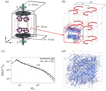
The von Kármán experiment (denoted herein as EXP) consists of two facing disks of diameter  $D=19$ cm (equal to the forcing-based integral scale,
 $L_{F}^{EXP}$), with eight straight blades each, separated by a vertical distance of
 $H=20$ cm. The impellers are in a cell of square cross-sectional size
 $(20 \times 20 \times 50)~{\rm cm}^3$ (room is left at the back of the impellers for shafts to connect them to motors, and for refrigeration coils to remove heat), filled with distilled water from a double-pass reverse osmosis system. The accessible experimental volume, in-between the two disks, is thus of
 $(20\times 20 \times 20)~{\rm cm}^3$. Each impeller is driven by a brushless rotary Yaskawa SMGV-20D3A61 servomotor, with Yaskawa SGDV-8R4D01A servo controllers (see Angriman et al. (Reference Angriman, Mininni and Cobelli2020) for further details). The two impellers rotate in opposite directions with angular velocity
 $\pm 2{\rm \pi} f_0$ (
 $f_0 = 50$ revs per minute). This generates two large counter-rotating circulation cells producing, on average, a strong shear layer at the midplane between the disks. A secondary circulation in the axial direction is also generated by the impellers, resulting in a 3-D turbulent flow with an anisotropic large-scale mean flow (depicted schematically in figure 1). We seeded this flow with inertial particles of radius
 $R = 3$ mm, which are plastic spheres with density
 $1.02$ times the fluid density, 3-D-printed using acrylonitrile butadiene styrene (known as ABS). The particles radius is such that
 $R/\lambda = 0.77$ and
 $R/\eta = 31$, with
 $\lambda$ the Taylor microscale and
 $\eta$ the Kolmogorov length scale (see table 1 for definitions). Measurements of particles’ dynamics were carried out in a large observation volume
 $V_{obs}^{EXP}$ of size
 $(16 \times 16 \times 16)~\text {cm}^3$, centred about the geometrical midpoint of the cell, using particle tracking velocimetry with two high-speed Photron FASTCAM SA3 cameras at a sampling rate of 125 frames per second. In total we have
 $O(10^5)$ frames. In each frame the mean number of particles simultaneously recorded is
 $11$, while their maximum recorded number is
 $29$ (note particles can exit and re-enter the observation volume, exploring also the regions behind the impellers).
(a) Experimental set-up, (b) TG and (d) HIT simulations. In the 3-D renderings (done with VAPOR; Clyne et al. (Reference Clyne, Mininni, Norton and Rast2007)), the blue lines are streamlines. For the TG simulation in (b), streamlines are shown in one ‘VK cell’, streamlines in the other cells are similar. The curved red arrows indicate the TG forcing direction. (c) Eulerian energy spectrum for TG and HIT direct numerical simulations (DNSs), Kolmogorov scaling is shown as a reference.

Parameters for the experiment (EXP), and for TG and HIT DNSs. Here  $\lambda = (15 \nu U^2/\varepsilon )^{1/2}$ is the Taylor microscale, with
 $\nu$ the kinematic viscosity,
 $\varepsilon$ the energy injection rate,
 $U$ the root mean square velocity and
 $\eta = (\nu ^3/\varepsilon )^{1/4}$ is the Kolmogorov length scale, both normalized by the forcing scale
 $L_{{F}}$;
 ${Re}_\lambda = U \lambda /\nu$ and
 ${Re} = U L_{{F}}/\nu$ are the Taylor and integral scale Reynolds numbers, respectively;
 ${St}$ and
 ${Re}_p = 2R |\boldsymbol {u} - \boldsymbol {v}|/\nu$ are the particles Stokes and Reynolds numbers;
 $\sigma_{\mathcal V}/\sigma _{RPP}$ is the ratio of standard deviations of the normalized Voronoï volumes to those from a random Poisson process (RPP), while
 $\langle V_c \rangle ^{1/3}$ is the mean linear cluster size, for STPS (S), ZAPS (Z), WZERO (W) and PART (P).

We also performed DNSs of the Navier–Stokes equations
 \begin{equation} \partial_t {\boldsymbol u} +{\boldsymbol u}\boldsymbol{\cdot}{\boldsymbol \nabla}{\boldsymbol u} ={-}{\boldsymbol \nabla}p +\nu \nabla^{2}{\boldsymbol u}+{\boldsymbol F}, \end{equation}
where  ${\boldsymbol u}$ is the solenoidal fluid velocity field (
 $\boldsymbol {\nabla } \boldsymbol {\cdot} {\boldsymbol u}=0)$,
 $p$ is the pressure per unit mass density,
 $\nu$ is the kinematic viscosity and
 ${\boldsymbol F}$ is an external volumetric mechanical forcing. Equations are written in dimensionless units based on a unit length
 $L_0$ and a unit velocity
 $U_0$, and solved in a 3-D
 $2{\rm \pi}$-periodic cubic box using a parallel pseudospectral method with the GHOST code (Mininni et al. Reference Mininni, Rosenberg, Reddy and Pouquet2011; Rosenberg et al. Reference Rosenberg, Mininni, Reddy and Pouquet2020). A fixed spatial resolution of
 $N^3 = 768^3$ grid points is used. To mimic the geometry of the large-scale flow in the von Kármán experiment, the external forcing
 ${\boldsymbol F}$ is given by the TG flow,
 \begin{equation} {\boldsymbol F}_{TG} = F_0 \left[ \sin(x) \cos(y) \cos(z) \, \hat{x} - \cos(x) \sin(y) \cos(z) \, \hat{y} \right] . \end{equation}
This forcing corresponds to a periodic array of counter-rotating large-scale vortices, which in the domain  $[0,{\rm \pi} )\times [0,{\rm \pi} )\times [0,{\rm \pi} )$ reduces to just two counter-rotating vortices separated vertically by a shear layer (see figure 1, where we call this domain a ‘VK cell’ by analogy with the von Kármán flow). We also performed a simulation of HIT with random forcing, to compare with the TG DNS and EXP. The HIT simulation was performed following the same procedures used for the TG DNS, using a spatial resolution of
 $768^3$ grid points. Turbulence was sustained by injecting energy in all modes in the vicinity of the Fourier shell with wavenumber
 $k = 1$, with constant solenoidal amplitude and random phases, i.e. the forcing
 ${\boldsymbol F}$ is given by
 \begin{equation} {\boldsymbol F}_{HIT} = F_0 \sum_{|{\boldsymbol k}|\in(0,2)} {\mathrm{Re}} \left\{ \frac{{\rm i} \, {\boldsymbol k} \times \hat{\boldsymbol e}_{\boldsymbol k}}{|{\boldsymbol k}|} \exp\left({{\rm i}({\boldsymbol k} \boldsymbol{\cdot} {\boldsymbol r} + \phi_{\boldsymbol k})}\right) \right\} , \end{equation}
where  ${\mathrm {Re}}$ denotes real part,
 $\hat {\boldsymbol e}_{\boldsymbol k}$ is a unit vector and
 $\phi _{\boldsymbol k}$ is a random phase. The random phases for each mode are slowly evolved in time, with a correlation time of
 $0.5$ large-scale eddy turnover times. For the TG DNS the magnitude of the forcing wavenumber satisfies
 $|\boldsymbol {k}_{F}^{TG}| = \sqrt {3}$, so the forcing length scale is defined as
 $L_{F}^{TG} = 2{\rm \pi} /|\boldsymbol {k}_{F}^{TG}| = 2{\rm \pi} /\sqrt {3}$, while for HIT
 $|\boldsymbol {k}_{F}^{HIT}| = 1$, and then
 $L_{F}^{HIT} = 2{\rm \pi}$ (see table 1 for relevant parameters).
In both simulations we integrate a minimal model of heavy inertial point particles, satisfying the effective equations of motion
 \begin{equation} \dot{\boldsymbol x}_p = {\boldsymbol v}(t) , \quad \dot{\boldsymbol v} = [{\boldsymbol u}({\boldsymbol x}_p,t) - {\boldsymbol v}(t)]/{\tau_p}, \end{equation}
where  ${\boldsymbol v}(t)$ and
 $\tau _p$ are the particles velocity and Stokes time, respectively. As the particles radius in EXP is such that the Maxey–Riley approximation is not valid (see, e.g. Qureshi et al. (Reference Qureshi, Bourgoin, Baudet, Cartellier and Gagne2007), Calzavarini et al. (Reference Calzavarini, Kerscher, Lohse and Toschi2008), Volk et al. (Reference Volk, Calzavarini, Verhille, Lohse, Mordant, Pinton and Toschi2008) and Homann & Bec (Reference Homann and Bec2010) for detailed studies of limitations of this approximation, and of (2.4a,b) in particular), and as the equations of motion of our particles are not known, (2.4a,b) should be considered as a model with effective parameters, or as a reference model to compare with, to determine whether the clustering of the particles in the experiment resembles the one expected from clustering mechanisms in the case of inertial particles. Note also that, while higher-order terms in the particles radius of the full Maxey–Riley equations could be considered (for instance, considering added mass forces, as done by Calzavarini et al. (Reference Calzavarini, Kerscher, Lohse and Toschi2008), or keeping Faxén corrections (Calzavarini et al. Reference Calzavarini, Volk, Bourgoin, Lévêque, Pinton and Toschi2009) and Basset–Boussinesq forces (Brennen Reference Brennen2005)), the particles in the experiment have
 $R \gg \eta$, and therefore the perturbative expansion in
 $R$ in the Maxey–Riley approximation is not valid (indeed, neutrally buoyant particles slightly larger than
 $\eta$ in such approximation do not cluster, see, e.g. the studies in Calzavarini et al. (Reference Calzavarini, Kerscher, Lohse and Toschi2008) and Reartes & Mininni (Reference Reartes and Mininni2021)). We thus regard (2.4a,b) simply as an effective equation with only one tunable parameter. For a brief analysis of how other forces affect the clustering of particles, see appendix A.
The tunable parameter in (2.4a,b) depends on the Stokes number of the particles in EXP. For finite-size particles, it is known that their dynamics can depend on many parameters (Fiabane et al. Reference Fiabane, Zimmermann, Volk, Pinton and Bourgoin2012), and that the conventional definition of the Stokes number does not properly characterize the particles’ dynamics (Xu & Bodenschatz Reference Xu and Bodenschatz2008; Fiabane et al. Reference Fiabane, Zimmermann, Volk, Pinton and Bourgoin2012). Let us consider the Stokes number  ${St} = \tau _p/\tau _f$, where
 $\tau _p$ is the particle's response time, and
 $\tau _f$ is some characteristic time of the flow. Using the standard definition of the viscous relaxation time of the particle (Cartwright et al. Reference Cartwright, Feudel, Károlyi, de Moura, Piro and Tél2010),
 \begin{equation} \tau_p^{v} = \frac{2}{9} \left( \frac{\rho_p}{\rho_f} + \frac{1}{2} \right) \frac{R^2}{\nu}, \end{equation}
where  $\rho _p/\rho _f$ is the particle-to-fluid mass density ratio, and setting
 $\tau _f$ as the Kolmogorov time scale
 $\tau _\eta$, for the particles in EXP we obtain
 ${St}_v^{{EXP}} = \tau _p^v/\tau _\eta = 312$. This choice would result in particles almost decoupled from the fluid (i.e. with too much inertia) if used in (2.4a,b).
To calculate an effective  $\tau _p$ for EXP we then set the Stokes number as
 ${St} = \tau _p/\tau _\eta$ and we estimate an effective particle time
 $\tau _p^{EXP} = (R^2/\varepsilon )^{1/3}$ as the turbulent turnover time at the particle radius (Angriman et al. Reference Angriman, Mininni and Cobelli2020). This choice can be understood as follows. For a spherical particle of radius
 $R$ and mass
 $m_p$ moving with velocity
 $\boldsymbol {v}$ in a uniform velocity field
 $\boldsymbol {u}$, the drag force
 $\boldsymbol {F}_D$ acting on the particle per unit mass can be estimated as (Batchelor Reference Batchelor2000)
 \begin{equation} \frac{\boldsymbol{F}_D}{m_p} = \frac{1}{2} \frac{\rho_p}{m_p}~ S~ C_D({Re}_p)|\boldsymbol{u} - \boldsymbol{v}|(\boldsymbol{u} - \boldsymbol{v}), \end{equation}
where  $\rho _p = 3 m_p/(4{\rm \pi} R^3)$ is the particle's density and
 $S = 4{\rm \pi} R^2$ represents its surface. Here
 $C_D({Re}_p)$ is the drag coefficient, which is a function of the particle Reynolds number, defined as
 ${Re}_p = 2 R |\boldsymbol {u} - \boldsymbol {v}|/\nu$. Then, (2.6) reads
 \begin{equation} \frac{\boldsymbol{F}_D}{m_p} = \frac{3}{2}\,C_D({Re}_p)\, \frac{|\boldsymbol{u} - \boldsymbol{v}|}{R}\,(\boldsymbol{u} - \boldsymbol{v}), \end{equation}
which can be approximated as  $\boldsymbol {F}_D/m_p \approx (\boldsymbol {u} - \boldsymbol {v})/\tau _p$, with
 \begin{equation} \tau_p \sim \frac{2}{3} \frac{1}{C_D({Re}_p)}~\frac{R}{\langle |\boldsymbol{u} - \boldsymbol{v}| \rangle}, \end{equation}
where angle brackets denote time averages. For finite-size neutrally buoyant particles, Cisse, Homann & Bec (Reference Cisse, Homann and Bec2013) estimated  $\langle |\boldsymbol {u} - \boldsymbol {v}| \rangle \sim (\varepsilon R)^{1/3}$, assuming Kolmogorov scaling and proposing a self-similar solution in the surroundings of the particle, and verified the validity of this estimation using DNSs. Substituting their result in (2.8) leads to
 \begin{equation} \tau_p \sim \frac{2}{3}\frac{1}{C_D({Re}_p)} ~ \left(\frac{R^2}{\varepsilon}\right)^{1/3}. \end{equation}
In EXP we can also estimate the particle–fluid slip velocity  $|\boldsymbol {u} - \boldsymbol {v}| \approx (|\langle u \rangle ^2 - \langle v \rangle ^2|)^{1/2}$ from the 3-D root mean square flow and particles’ velocities (Bellani & Variano Reference Bellani and Variano2012), which gives
 ${Re}_p \approx 400$. For this value of
 ${Re}_p$,
 $C_D \approx 0.6$ (Batchelor Reference Batchelor2000; Morrison Reference Morrison2013), and then the dimensionless prefactor
 $2/[3 C_D({Re}_p)] \approx 1.1$; thus, the particle response time
 $\tau _p^{{EXP}} = (R^2/\varepsilon )^{1/3}$ can be interpreted as an effective time that takes into account the mean effect of nonlinear drag corrections. This in turn yields
 ${St}^{EXP}=9.95$. Other alternative definitions of the Stokes number have been introduced in the literature. For instance, Xu & Bodenschatz (Reference Xu and Bodenschatz2008) and Schmitt & Seuront (Reference Schmitt and Seuront2008) propose to use
 $\tau _p = \tau _p^{v*} = (1/18) (\rho _p/\rho _f) (4R^2/\nu )$, and to set
 $\tau _f$ as the turbulent dynamic time at the scale of the particle, i.e.
 $\tau _f = (4R^2/\varepsilon )^{1/3}$. For the EXP data this yields
 ${St}^{EXP}_{v*} = \tau _p^{v*}/\tau _R = 14$, which is of the same order of magnitude as our estimation.
In the DNSs,  $\tau _p$ is set equal to
 $\tau _p^{EXP}$ in units of
 $\tau _\eta$ (i.e. we set the same Stokes number
 ${St}$ within statistical fluctuations). In other words, given the values of
 $\tau ^{DNS}_\eta$ in the simulations, and of the Stokes number
 ${St}^{EXP}$ in the experiment, we set
 $\tau _p$ in (2.4a,b) as
 $\tau ^{DNS}_p = {St}^{EXP} \tau ^{DNS}_\eta$. An effective radius of the particles in the DNSs can then be estimated consistently with (2.9) as
 $R = [\varepsilon (\tau _p^{DNS})^3]^{1/2}$, and to compute the value of
 ${Re}_p$ reported in table 1 for the simulations we use
 $\boldsymbol {u}$ and
 $\boldsymbol {v}$ for each particle at every instant. Note both the experimental and numerical estimations of the Reynolds particle number yield
 $Re_p \gg 1$, reinforcing the fact that models for particles of moderate size do not apply in our case, and that the equations for inertial particles in the DNSs should be understood only as a crude effective model. All the values of
 $St$ and
 $Re_p$ for EXP, TG and HIT data are listed in table 1.
3. Results
3.1. Voronoï volumes probability distribution
Nulls of all vector fields were computed in the DNSs using the methods described in Haynes & Parnell (Reference Haynes and Parnell2007) and Mora et al. (Reference Mora, Bourgoin, Mininni and Obligado2021). Using the positions of the zeros, and the particles’ positions in the experiment and DNSs, 3-D Voronoï tessellations were computed for all datasets. While the DNSs use  $10^6$ particles, in the experiment we have a maximum of
 ${\approx }29$ particles in each frame, resulting in a significantly smaller number of closed 3-D Voronoï cells; there are an average of three closed cells per snapshot. When considering all snapshots this results in a total number of closed cells of
 $1.9\times 10^5$. Also, in DNSs, the tessellations were performed with periodic boundary conditions. These two observations will be relevant in interpreting some of the results.
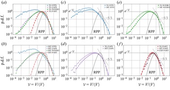
Figure 2 shows the probability density functions (p.d.f.s) of the normalized volumes of the Voronoï cells,  ${\mathcal V} = V/\langle V \rangle$, for STPS, ZAPS and ZWEROs in TG and HIT, and the p.d.f.s of the Voronoï cells for the particles in the DNSs and the experiment. For the experimental data, since the total number of particles fluctuates in time (as particles can enter or exit the observation volume
 $V_{obs}^{EXP}$, and as already mentioned, can explore regions behind the disks),
 $\langle V \rangle _{EXP}$ is defined as the volume occupied by the fluid between the propellers divided by the mean number of particles per image, calculated from all of the available images. This choice is robust to variations in the number of particles (Fiabane et al. Reference Fiabane, Volk, Pinton, Monchaux, Cartellier and Bourgoin2013), and to the presence of spurious volumes near the boundaries of the images as will be discussed later.
The p.d.f.s of normalized Voronoï volumes,  ${\mathcal V} = V/\langle V \rangle$, for STPS, ZAPS, WZERO and inertial particles positions (PART). Panels (a,b) show a comparison of all quantities in TG and HIT. The p.d.f.s of (c) STPS, (d) ZAPS and (e) WZERO for TG and HIT. (f) The p.d.f.s of PART for TG, HIT and EXP. A RPP, an exponential and a
 $-5/3$ power law are shown as references.

It has been hypothesized that the forcing mechanism or the large-scale flow can introduce changes in the clustering of nulls of the fluid vector fields (Goto & Vassilicos Reference Goto and Vassilicos2009). This figure confirms this is indeed the case: HIT displays stronger clustering of all fields than TG (i.e. larger probabilities for small volumes). In the figures, the p.d.f. resulting from a RPP (corresponding to homogeneous distribution of nulls or particles) is shown as a reference. The larger standard deviation of the p.d.f.s (compared with the RPP, whose standard deviation is  $\sigma _{RPP} \approx 0.42$) and the stronger tails (of clusters to the left, and of voids to the right) indicate enhanced clustering. However, the Voronoï cell volumes of the particles is similar for the three flows, and notably, the level of clustering as quantified by
 $\sigma _{\mathcal V}$ is similar for TG and EXP (see table 1). As will be discussed next, differences between EXP and TG can be associated with finite sampling and with boundary effects.
In figure 2 we also show an exponential and a  $-5/3$ power law to serve only as references for the comparison. Note STPS in HIT are more similar to the
 ${\mathcal V}^{-5/3}$ power law in the vicinity of
 ${\mathcal V} \approx 1$ (i.e. for intermediate volumes, their distribution is closer to a power law than to an exponential decay), which is a consequence of the power-law behaviour of the velocity autocorrelation function (Davila & Vassilicos Reference Davila and Vassilicos2003; Smith, Hopcraft & Jakeman Reference Smith, Hopcraft and Jakeman2008). The TG STPS display a less clear scaling, which is compatible with contamination of the scaling of the velocity by the mean flow (Angriman et al. Reference Angriman, Mininni and Cobelli2020). The ZAPS and WZERO do not exhibit a power law behaviour, and are closer to an almost exponential decay
 $\sim {\rm e}^{-{\mathcal V}}$ in all DNSs for large volumes (i.e. for
 ${\mathcal V}>1$), with the aforementioned differences between HIT and TG for very small values of
 ${\mathcal V}$. Remarkably, the p.d.f.s of Voronoï cells of all particles are very similar in spite of the differences in the distribution of zeros, and for intermediate and large volumes (
 ${\mathcal V} \gtrsim 1$) are closer to an exponential decay, indicating the clustering of particles for those volumes is more akin to the distribution of either ZAPS or WZERO than to the distribution of STPS. It is worth recalling that some studies of finite-size, neutrally buoyant particles in HIT laboratory flows indicate that small particles do not cluster and behave as tracers (Fiabane et al. Reference Fiabane, Zimmermann, Volk, Pinton and Bourgoin2012), at least from a Voronoï tessellation point of view. Fiabane et al. (Reference Fiabane, Zimmermann, Volk, Pinton and Bourgoin2012) considered neutrally buoyant particles whose radii ranged from
 $2.25\eta$ to
 $8.5\eta$ (
 $0.0875\lambda$ to
 $0.23\lambda$). The particles employed here are well outside this range, with a size comparable to the Taylor microscale, a scale at which viscous effects from the turbulent flow become less relevant. Our results suggest that Taylor-scale neutrally buoyant particles cluster similarly to inertial particles. The numerical particle data thus serve the purpose of gauging the level of clustering the experimental particles experience when compared with the minimal model in the simulations. As particles in the DNS cluster akin to different flow nulls, the comparison allows us to further relate the clustering in the experiment with specific properties of the background flow.
3.2. Biases in the evaluation of Voronoï tessellation using particles’ positions
Measurement of 3-D clustering in experiments poses multiple challenges. Particle seeding must be sufficiently small to remain in the regime of a dilute suspension (Elghobashi Reference Elghobashi1994), which results in a few particles per measurement. When computing 3-D Voronoï tessellations, this results in a small number of closed cells, roughly proportional to the cube root of the total number of detected particles. Thus, the number of closed Voronoï cells scales slowly with the number of particles (see Tagawa et al. (Reference Tagawa, Mercado, Prakash, Calzavarini, Sun and Lohse2012) for another study of 3-D clustering in experiments). Lastly, boundaries have a drastic effect on the statistics. In this section we compare DNSs, synthetically post-processed DNSs and laboratory data, to quantify the effect of these ever-present limitations. We therefore evaluate possible sources of biases in the 3-D Voronoï tessellation calculated from the inertial particles’ instantaneous positions by processing DNS data so as to mimic experimental conditions.
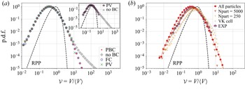
We first focus on the effect of boundaries. Particles near the boundaries of the observation region in the experiment occupy either open cells (which are always discarded in the analyses) or artificially large cells, as particles closing their cells (or the domain walls) are not visible in the cameras field of view. The result is depicted in figure 3(a) (inset), which shows the Voronoï tessellation on the raw EXP data without imposing any restriction on the cells near boundaries (labelled ‘no BC’ in the figure); note the power-law tail for very large  ${\mathcal V}$. We reproduced this situation in the TG DNS by computing the tessellation imposing periodic boundary conditions (‘PBC’, considered as ground truth), by imposing no condition on the boundaries (‘no BC’, which results in a power-law dependence), by removing all cells close to boundaries (labelled ‘FC’ in the figure), and by dropping the largest cells that resulted in a total volume larger than the observation volume (that is, keeping only ‘physical’ volumes, ‘PV’), see figure 3(a). The latter method, when applied to EXP data, results in the p.d.f. shown in the inset of figure 3(a) (the strategy also used in figure 2f). In each case,
 $\langle V \rangle$ is the total volume occupied by the fluid divided by the mean number of particles, to remove biases (especially when large spurious volumes are kept). Boundaries mainly affect the statistics of large cells, but the left tails of the p.d.f.s remain the same regardless of the strategy used for treating the boundaries. This suggests boundaries do not affect significantly the determination of clusters (as clusters are formed by small volumes
 ${\mathcal V}$ below some threshold, as will be discussed in the following section). Furthermore, we verified that when analysing DNS data in the same way as EXP data (i.e. by considering the non-periodic VK cells in the TG DNS and keeping only ‘physical’ Voronoï cells), the distribution of cluster volumes reported in the following section remains unchanged.
(a) The TG data tessellated without any boundary conditions (no BC), with periodic boundary conditions (PBC), removing frontier cells (FC) or keeping only physical volumes (PV). Inset shows EXP data. Note the spurious tails for large  ${\mathcal V}$. (b) The TG data subsampled to 250 or 5000 particles, and subsampled in only a VK cell with an average of 13 particles, is compared with the tessellation keeping all particles and to EXP data. Note the lower probability of small volumes when subsampling.

The relatively low number of particles in experiments also has an effect on the p.d.f.s. Figure 3(b) shows EXP data together with the original TG data (tessellated using periodic boundary conditions), and the TG data subsampled to a maximum of 250 and 5000 particles. These subsampled sets were built so as to follow the same distribution of number of particles per frame as in the experiments. This was done in the following way. The maximum number of particles  $N_{max}$ considered (either 250 or 5000) represents the DNS-equivalent of the total number of particles inside the experimental vessel (but not necessarily within the observation volume at once); e.g.
 $N_{max} = 250$ corresponds to roughly 31 particles available in each of the eight individual VK cells that the DNS comprises. The experimental variability in the actual number of particles that simultaneously occupy the observation volume at any time instant was mimicked in these numerical datasets based on the occupation probability distribution (i.e. the probability of observing a certain number of particles at each time instant), which was calculated empirically from the EXP data. As a result, for
 $N_{max} = 250$, the mean number of particles per frame in the complete numerical domain of volume
 $(2{\rm \pi} )^3$ is
 $\approx 111$, leading to approximately 13 particles per VK cell of the TG flow, comparable to what is attained in the experiments. These subsampled datasets were then processed in a manner identical to what was done with the experimental data; namely, employing a tessellation scheme without considering periodic boundary conditions and keeping only physical volumes in the entire
 $(2{\rm \pi} )^3$ domain. To further mimic the experimental conditions, the subsampling of the TG data was also performed in one VK cell, i.e. in just the octant comprised by the subdomain
 $[0,{\rm \pi} )\times [0,{\rm \pi} )\times [0,{\rm \pi} )$, thus keeping an average of only 13 particles per snapshot. The tessellation was then carried out as in the case of
 $N_{max} = 250$ and
 $N_{max} = 5000$ but in the smaller subdomain; the resulting p.d.f. is shown in figure 3(b) as well.
Decreasing the number of particles in the DNS in these ways – in both the ( $2{\rm \pi} )^3$ domain and in the VK cell – as shown in figure 3(b), results in p.d.f.s whose left tails slowly move towards the RPP, partially explaining the slight defect of small volumes
 ${\mathcal V}$ seen in the EXP data. The reduction in the number of particles, and the treatment of boundaries discussed above, also has a small effect in the concavity of the right tail of the observed p.d.f. For a detailed study of other experimental biases in two-dimensional (2-D) Voronoï tessellation, including subsampling effects, see Monchaux (Reference Monchaux2012), and for an investigation of finite-size effects on Voronoï analysis of randomly placed spheres, see Uhlmann (Reference Uhlmann2020).
3.3. Effect of preferential sampling of large-scale inhomogeneities in the experiment
While small (larger than the Kolmogorov scale) particles do not cluster (Fiabane et al. Reference Fiabane, Zimmermann, Volk, Pinton and Bourgoin2012), neutrally buoyant particles with sizes of the order of the flow integral scale have been reported to cluster in von Kármán experiments (Machicoane et al. Reference Machicoane, Zimmermann, Fiabane, Bourgoin, Pinton and Volk2014). The clusters in that case were found to be associated with large-scale flow inhomogeneities (i.e. preferential sampling by the particles) and with confinement effects (Machicoane et al. Reference Machicoane, López-Caballero, Fiabane, Pinton, Bourgoin, Burguete and Volk2016), rather than with inertial effects. It is then worth analysing whether the clustering behaviour observed in our finite-size particles is the result of, or at least affected by, a global preferential sampling such as the one reported by Machicoane et al. (Reference Machicoane, Zimmermann, Fiabane, Bourgoin, Pinton and Volk2014). To this end we computed the 3-D spatial concentration map  $C({\boldsymbol {x}})$ of the particles in the experiment, using all available snapshots and normalized so that the average in the entire observation volume is
 $\langle C({\boldsymbol {x}})\rangle _{V_{obs}^{EXP}} = 1$. Figure 4(a,b) show 2-D probability density maps of the particles’ positions (proportional to the 2-D concentration maps) in the
 $x$–
 $z$ and
 $y$–
 $z$ planes, respectively, where
 $\hat {z}$ is chosen parallel to the rotation axis of the propellers and to the direction of gravity. Our particles present a more uniform distribution than the larger particles considered in Machicoane et al. (Reference Machicoane, Zimmermann, Fiabane, Bourgoin, Pinton and Volk2014) and Machicoane et al. (Reference Machicoane, López-Caballero, Fiabane, Pinton, Bourgoin, Burguete and Volk2016). This is consistent with previous observations: in Machicoane et al. (Reference Machicoane, Zimmermann, Fiabane, Bourgoin, Pinton and Volk2014) the larger particles are the ones that display the stronger inhomogeneous preferential sampling, while their smaller particles (with
 $R /\lambda \approx 2.6$) sample the flow more uniformly than their larger particles. In spite of this, in figure 4 a very small tendency for our particles to be in the lower half of the cell (
 $z < 0$) can still be observed, especially near the corners. This may be partially due to asymmetries in the position of the shear layer in the von Kármán flow (Ravelet et al. Reference Ravelet, Marié, Chiffaudel and Daviaud2004; Huck et al. Reference Huck, Machicoane and Volk2017), to a small effect of gravity, and to the particles entering and exiting the region behind the propellers; the latter effect is particularly visible in the lower corners of the concentration maps.
The 2-D p.d.f.s of inertial particles positions in EXP, (a)  $x$–
 $z$ plane and (b)
 $y$–
 $z$ plane, where
 $\hat {z}$ is parallel to the axis of rotation of the propellers. (c) The p.d.f. of the original normalized Voronoï volumes for EXP, same p.d.f. compensating each volume by the concentration at the corresponding particle position
 $C_0=C({\boldsymbol x}_0)$ (i.e. p.d.f. of
 ${\mathcal V}C_0$), and compensating by the average concentration in each volume
 $\langle C \rangle =\langle C ({\boldsymbol x})\rangle _{\mathcal V}$.

To quantify the effect that the particles’ preferential sampling has on the observed clustering, we computed the Voronoï cells compensating each cell volume  ${\mathcal V}$ by its local particle concentration. The purpose of doing this is to correct any underestimation (overestimation) of the cell volumes resulting from the cells being located in regions of space with higher (lower) particle concentration. This can be done in two ways. For a given particle located at
 ${\boldsymbol {x}_0}$, the volume of its Voronoï cell
 ${\mathcal V}$ can be multiplied by the concentration at the particle position
 $C({\boldsymbol {x}_0})$, i.e.
 ${\mathcal V} C(\boldsymbol {x}_0)$, or by the average concentration in the entire cell that contains that particle
 $\langle C({\boldsymbol x}) \rangle _{\mathcal V}$, i.e.
 ${\mathcal V} \langle C \rangle _{\mathcal V}$. We thus computed p.d.f.s using these two compensated cell volumes, which are shown in figure 4(c) along with the p.d.f. of
 ${\mathcal V}$ without any compensation. The overall shape of the p.d.f.s remain similar, with the heavy tails that deviate from the RPP being preserved. The second compensation, using the mean concentration in each cell, does not change significantly the distribution of large volumes, but does decrease slightly the probability of finding small volumes. Even so, the compensated p.d.f.s indicate that large-scale sampling effects as reported in Machicoane et al. (Reference Machicoane, Zimmermann, Fiabane, Bourgoin, Pinton and Volk2014) play a smaller role in our case, and confirm that the clustering observed in the experiment is at least partially associated with inertial effects. As a reference, the standard deviation of the Voronoï volumes compensated by
 $\langle C \rangle _{\mathcal V}$ is
 $\sigma _{{\mathcal V}_{\langle C \rangle }}/\sigma _{{RPP}} \approx 2.73$, which is slightly larger than
 $\sigma _{\mathcal V}/\sigma _{{RPP}} \approx 2.33$ for the uncompensated Voronoï volumes in the experiment (see table 1), and closer to the reference value for the minimal model of inertial particles in the TG DNSs.
3.4. Cluster volumes probability distribution
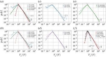
Figure 5 shows the p.d.f.s of the volumes of the clusters  $V_c$ (formed by at least two adjacent cells with
 ${\mathcal V}<{\mathcal V}_c$, where
 ${\mathcal V}_c$ is the first crossing between the p.d.f. of
 ${\mathcal V}$ with the RPP, see Monchaux et al. (Reference Monchaux, Bourgoin and Cartellier2010)), for all vector fields nulls and for the particles, in the DNSs and EXP. From Mora et al. (Reference Mora, Bourgoin, Mininni and Obligado2021) we expect a
 $V_c^{-5/3}$ scaling for STPS, and
 $V_c^{-2}$ for ZAPS and WZEROs, resulting from the fractal nature of the spatial distribution of these zeros. Hence, the presence or not of these power laws provides information about the clusters geometry and their fractality (see Obligado et al. (Reference Obligado, Teitelbaum, Cartellier, Mininni and Bourgoin2014) and Mora et al. (Reference Mora, Bourgoin, Mininni and Obligado2021) for simple models and a review of the origin of these power laws). For all nulls, HIT shows a slight excess of smaller volume clusters when compared with TG, but overall the p.d.f.s and scalings are similar.
The p.d.f.s of the cluster volumes normalized by the average Voronoï volume,  $V_c/\langle V \rangle$, for STPS, ZAPS, WZERO and PART, in DNSs and EXP. Labels for the panels are as in figure 2. Panel (f) also shows the EXP data when corrected by the mean concentration per volume
 $\langle C \rangle$. The normalized observation volume in EXP is indicated by an arrow in the same panel. Power laws with exponents
 $-5/3$ and
 $-2$ are shown as references.

Figure 5(f) also shows the p.d.f.s of  $V_c$ for particles in the DNSs and EXP (in the latter case, with and without corrections by the mean average concentration per volume), which are expected to follow a
 $-2$ power-law scaling, with a shorter range as a result of the large
 ${St}$ considered. Clusters of particles in the experiment have different p.d.f.s than in TG or HIT. The right tails of the p.d.f.s in the experiment, associated with volumes
 $V_c > \langle V \rangle$, present a sharp drop, as the cluster size cannot be larger than the observation volume (
 $V_{obs}^{EXP}/\langle V \rangle$ is indicated by the arrow in the figure). On the other hand, in the p.d.f. of uncompensated EXP volumes, the probability of having small clusters (with
 $V_c < \langle V \rangle$) is larger than in the DNSs. We verified that this is not an effect of subsampling or boundaries, so this difference underlines limitations in the scope of the toy model considered in (2.4a,b) and, ultimately, in the effect of the mean large-scale flow as captured by the model, either from missing physical effects or from preferential sampling. Neglected interactions between particles is not the probable cause, as the volumetric loading ratio is
 $\lesssim 2\times 10^{-4}$. However, particles in the DNSs, while subjected to Stokes drag, are point particles that can only sense pressure gradients indirectly through the carrier velocity field. On the other hand, finite-size particles are expected to sense the pressure gradient directly as a force acting on their surface, as well as velocity gradients (and thus, shear stresses) that the point particles in the DNSs cannot sense. Pressure gradients have already been pointed out as important in the understanding of the formation of clusters of finite-size particles (Fiabane et al. Reference Fiabane, Zimmermann, Volk, Pinton and Bourgoin2012). Finally, when compensating each EXP particle volume by the mean concentration, the probability of finding smaller clusters decreases and becomes closer to that of the model, suggesting that the small preferential concentration induced by the large-scale flow geometry plays a role here. This is confirmed by the fact that small and large clusters in TG and EXP flows occur at slightly different places, which could also explain why their p.d.f.s look different.
In table 1 a comparison of the mean linear cluster size  $\langle V_c\rangle ^{1/3}$ for all quantities is given, normalized by
 $\eta$. The mean linear cluster sizes of WZERO and ZAPS are similar for TG and HIT, but STPS clusters are slightly larger for HIT, a difference that may be related to the fact that the HIT forcing scale is larger than in TG, and thus larger clusters may appear. The mean linear cluster size of particles in EXP is much larger than in TG or HIT. Even when conditioning the data as discussed in § 3.2 (that is, subsampling the number of particles in the DNS, and considering boundary effects), or as in § 3.3 (i.e. correcting by the particles concentration), we observe that clusters in the experiment are still three times larger, on average, than in TG. This difference is associated with the finite volume of the particles in EXP. Note that finite-size particles can only form clusters with a minimum linear size of order
 $4R$, which for EXP data is greater than
 $120\eta$. In other words, some clusters in TG cannot be realized in the experiment without the actual particles overlapping.
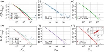
The p.d.f.s of the number of clusters  $M_c$ with
 $N_{PC}$ points inside each cluster are shown for the DNSs in figure 6. These p.d.f.s follow a power-law behaviour with an exponent close to
 $-16/9$ for STPS, and
 $-2$ for ZAPS and WZERO, as expected from Mora et al. (Reference Mora, Bourgoin, Mininni and Obligado2021). Figure 6(c) indicates that the probability of having clusters of STPS with a larger number of nulls is larger for HIT than for TG, consistent with the larger mean linear size of clusters of STPS in HIT. Inertial particles also follow a power law with an exponent close to
 $-2$ for clusters with
 $N_{PC} \lesssim 10$, a behaviour consistent with the one reported by Yoshimoto & Goto (Reference Yoshimoto and Goto2007). Overall, the observed scaling is similar for ZAPS, WZERO and inertial particles, which is compatible with the sweep-stick mechanism (Goto & Vassilicos Reference Goto and Vassilicos2008; Coleman & Vassilicos Reference Coleman and Vassilicos2009; Oka & Goto Reference Oka and Goto2021). The deviation from the power law observed for particles in figure 6(f) might relate to the fact that particles with large Stokes number filter out small flow scales. Indeed, these kinds of particles are expected to be less responsive to small scale motions in the fluid, so clusters with a larger number of particles around very dense nulls in the carrier flow are less likely to form. Finally, the inset in figure 6(f) shows the linear cluster size normalized by
 $L_F$, as a function of the number of particles per cluster for the inertial particles. Note the cluster size grows with the number of particles with a
 $1/3$ scaling.
Probability conditioned to having clusters with  $N_{PC}$ points for STPS, ZAPS, WZERO and PART in DNSs. Labels for all panels are as in figure 2. The linear cluster size, normalized by
 $L_F$ and as a function of
 $N_{PC}$ is shown in the inset of panel (f). Several power laws are shown as references.

4. Discussion
Comparison of clustering in numerical simulations of homogeneous isotropic turbulence and TG turbulence with von Kármán experiments provides a powerful tool to characterize geometrical and topological properties of turbulence, and of multiphase flows. Moreover, the similarities between the TG flow and the laboratory von Kármán flow allow for detailed studies of possible biases when considering limitations in experiments such as low number of particles, boundary effects or the effect of preferential sampling of the large-scale flow by the particles.
Our results also show that 3-D Voronoï tessellation constitutes a powerful tool to study the topology of nulls and clusters, shedding light on dominant effects in the dynamics of the flow. For the case of the TG and von Kármán flows, these are: (1) a lower probability of finding very densely packaged zeros of the velocity field, the vorticity, and of the Lagrangian acceleration in the TG flow when compared with HIT; (2) a deviation in the scaling of the number of Voronoï volumes of STPS with  ${\mathcal V}$ in the TG flow, probably associated with the effect of the mean flow on the velocity autocorrelation function; (3) similar clustering properties of a minimal model of inertial particles in TG and of neutrally buoyant Taylor-scale particles in von Kármán flows as in inertial particles in HIT, probably resulting from the negligible differences (for intermediate cell volumes
 ${\mathcal V}$) in the statistics of ZAPS and WZERO observed in TG and HIT.
In the experiment, we find that particles with a size comparable to the Taylor microscale form clusters that are very similar in intensity and size distribution as the point particles in the simulations. This contrasts with previous results, for particles whose sizes were a fraction of  $\lambda$, and which did not exhibit clustering (Qureshi et al. Reference Qureshi, Bourgoin, Baudet, Cartellier and Gagne2007; Fiabane et al. Reference Fiabane, Zimmermann, Volk, Pinton and Bourgoin2012, Reference Fiabane, Volk, Pinton, Monchaux, Cartellier and Bourgoin2013), while close to point particles in experiments were found to form clusters (Obligado et al. Reference Obligado, Volk, Mordant and Bourgoin2019), as well as much larger particles (Machicoane et al. Reference Machicoane, Zimmermann, Fiabane, Bourgoin, Pinton and Volk2014, Reference Machicoane, López-Caballero, Fiabane, Pinton, Bourgoin, Burguete and Volk2016) were also found to cluster for different reasons. This points towards the possibility that intermediate, Taylor-scale neutrally buoyant particles cluster as a result of inertial effects.
These results are promising as they further confirm TG and von Kármán flows share many geometrical and statistical properties, even when considering preferential concentration of particles in multiphase turbulence. Moreover, they indicate that many clustering properties of HIT can be extended to multiscale flows with a large-scale circulation, at least in cases in which turbulent fluctuations are large (as in the TG and VK flows). Further studies will consider other forcing mechanisms and different large-scale geometries.
Acknowledgements
The authors thank D. Mora for help with data analysis of nulls calculation. The authors gratefully acknowledge suggestions by an anonymous referee of studying the spatial concentration map of the particles in the experiment.
Funding
This work has been partially supported by ECOS-Sud project no. A18ST04. S.A., F.Z., P.J.C. and P.D.M. acknowledge support from UBACYT grant no. 20020170100508BA and PICT grant no. 2018-4298. A.F. and M.O. acknowledge the LabEx Tec21 (Investissements d'Avenir – Grant Agreement no. ANR-11-LABX-0030).
Declaration of interests
The authors report no conflict of interest.
Appendix A. Models with other forces and their effect on clustering
In this appendix we briefly consider other possible models for the equations of motion of particles in the simulations. On the one hand we consider particles subjected to a nonlinear drag force as in Wang & Maxey (Reference Wang and Maxey1993), whose equations of motion read
 \begin{equation} \dot{\boldsymbol x}_p = {\boldsymbol v}(t) , \quad \dot{\boldsymbol v} = \frac{1 + 0.15 {Re}_p^{0.687}}{\tau_p} (\boldsymbol{u} - \boldsymbol{v}), \end{equation}
where  ${Re}_p = \sqrt {18\tau _p/\nu }|\boldsymbol {u} - \boldsymbol {v}|$. On the other hand we consider the Maxey–Riley equation (Maxey & Riley Reference Maxey and Riley1983) up to terms linear in the particle's radius, that is, we consider the Stokes drag, gravity and particle acceleration and added mass effects (and therefore neglecting Faxén corrections and the Basset–Boussinesq history term). Thus, particles evolve according to
 \begin{equation} \dot{\boldsymbol x}_p = {\boldsymbol v}(t) , \quad \dot{\boldsymbol v} = \frac{1}{\tau_p} ({\boldsymbol u} - {\boldsymbol v}) - g \frac{1 - \gamma}{1 + \gamma/2} \hat{z} + \frac{3}{2} \frac{\gamma}{1 + \gamma/2}~ \frac{{\rm D}\boldsymbol{u}}{{\rm D}t} , \end{equation}
where  $g$ is the gravitational acceleration,
 ${\rm D}/{\rm D}t = \partial /\partial t + {\boldsymbol u} \boldsymbol {\cdot} \boldsymbol {\nabla }$ and
 $\gamma = \rho _f/\rho _p$. Particles whose dynamics are governed by either (A1a,b) or (A2a,b) were evolved in the turbulent flow with TG mechanical forcing with a spatial resolution of
 $768^3$ grid points, following the same procedures as previously described for the TG DNSs. A total of
 $10^6$ particles were integrated. For the sake of comparison, and as both equations are missing other forces (see, e.g. Calzavarini et al. Reference Calzavarini, Kerscher, Lohse and Toschi2008, Reference Calzavarini, Volk, Bourgoin, Lévêque, Pinton and Toschi2009), we use in all cases the effective particle response time
 $\tau _p$ instead of the viscous relaxation time
 $\tau _p^v$, and in (A2a,b) we use
 $\gamma = 1/1.02 \approx 0.98$ and the value of
 $g$ to match the experiment. We performed a Voronoï tessellation of the particles’ positions, and the resulting cell volume's p.d.f.s are shown in figure 7, along with the p.d.f.s corresponding to particles evolving solely under Stokes drag as in (2.4a,b), and the experimental data. As expected, considering particle acceleration and added mass effects in the Maxey–Riley equation results in less clustering: (A2a,b) is well suited for smaller particles with small particle Reynolds number, which tend to cluster less (Fiabane et al. Reference Fiabane, Zimmermann, Volk, Pinton and Bourgoin2012, Reference Fiabane, Volk, Pinton, Monchaux, Cartellier and Bourgoin2013). Note in particular how the statistics of voids (i.e. of large Voronoï cells) approaches the statistics of the RPP; the standard deviation of this p.d.f. is
 $\sigma _{\mathcal V} = 1.31 \sigma _{RPP}$. Considering nonlinear drag as in (A1a,b) may be more relevant for particles of our size and with larger particle Reynolds number. This model results instead in more clustering, with a p.d.f. with
 $\sigma _{\mathcal V} = 2.92 \sigma _{RPP}$. The stronger clustering may be related to our choice of using an effective
 $\tau _p$. In the future, it may be of interest to compare nonlinear drag using the viscous response time of the particles (or other choices for the effective response time) against the simplified point particle model with the effective parameter in (2.4a,b). Note in particular that the results in figure 7 do not necessarily imply that (2.4a,b) is a better model for Taylor-scale neutrally buoyant particles, as to that end a more detailed comparison would be needed.
The p.d.f.s of normalized Voronoï volumes for inertial particles in a TG flow considering only Stokes drag as in (2.4a,b), the Maxey–Riley equation (with Stokes drag, gravity, particle acceleration and added mass effects) and nonlinear drag. The EXP data is shown as well for comparison.