

Introduction
The discourse on immigration in the United States is dominated by the “Ellis Island” narrative: a widespread perception about America's history of immigration that Europe's tired and poor (many of whom were from Southern or Eastern Europe) arrived with little more than change in their pockets, but managed with hard work and determination to achieve the American dream. That powerful image did more than crystallize the identity of the United States as a country of immigration. The Ellis Island narrative continues to frame scholarly and public discourse regarding the experience of contemporary immigrants. Perhaps the centrality of the narrative is seen in the introductory text of the Ellis Island National Monument, as represented by the US National Park Service:
America's “Golden Door”
They came seeking freedom, opportunity, new lives. More than 12 million immigrants passed through the doors of Ellis Island between January 1, 1892 and November 1954, hoping to achieve the “American Dream.” These people have woven their way into the fabric of American life. They have helped create the America we know today.
US National Park Service 2012
Of course, the Ellis Island narrative is very nonspecific. It often is taken to encapsulate a variety of features of change in the US setting: acculturation, socioeconomic advancement, new forms of citizenship, and a general integration into American life within and across generations. In our case, we concentrate on one key feature of the narrative, implicit in the reference to opportunity and the American Dream, in which upward socioeconomic mobility is the result for immigrants and the second generation. We do not argue against the narrative in this paper, but rather, we look for the subtleties in its manifestation (Fischer Reference Fischer2010) across the experience of origin groups. For whom and in what ways was the Ellis island narrative—upward mobility within and across generations—most apparent?
Although the current, that is early twenty-first century, period is described as one of record-level immigration for the United States, the demographic scale of immigration—in terms of percent foreign born—during the Ellis Island era was arguably larger (White and Glick Reference White and Jennifer Glick2009). The broad historical sweep of evidence is clear: the waves of late-nineteenth- and early-twentieth-century European immigrants did make their way successfully into US society, even despite concerns of inassimilability that grew in the wake of these boatloads of new arrivals. At the same time, our evidence on this point is aggregated and unrefined. Exactly how rapid was the rise? How did progress manifest itself across generations? How did different national origin groups fare? Embedded in the narrative about immigration are notions of responses to these questions, influencing current thinking in scholarly, lay, and policy circles. In this paper we aim to shed a brighter light on these questions and provide deeper empirical evidence of them. In particular, we aim to measure how much difference there was across time and between national origins for these newcomers to America's shores.
Consider the view expressed by Cecil Woodham-Smith (Reference Woodham-Smith1962: 207) in a classic historical work on the great Irish famine migration: “Very few of the poor Irish who fled from Ireland in the famine emigration were destined to achieve prosperity and success themselves. . . . It was not until the second or third generation that. . . the children and grandchildren of the poor famine immigrants became successful.” At base Woodham-Smith and others argue that it took multiple—many—generations for Ellis Island immigrants to enter the mainstream. Even mid-twentieth-century academic writing questioned the rate of assimilation of the Ellis Island wave. Writing with an eye toward policy, Hugh Carter in a Reference Carter1949 volume of the Annals (pp. 2–3) devoted to immigration offered: “Another important and frequently discussed factor in immigration policy is the assimilation of the foreign born. . . . One hears less today [Reference Carter1949] of the old and naive theory of the ‘melting pot’ according to which assimilation is both complete and rapid.”
Much more recent writing on immigration often hearkens back to the presumed experience of the Ellis Island era. Joel Perlmann, in his informatively titled Italians Then, Mexicans Now (Reference Perlmann2007 [2005]: 124), makes the explicit comparison between major groups of the Ellis Island era and the contemporary wave, respectively: “Because the Mexican second generation is faring less well in relative terms than its SCEN [Southern, Central, and Eastern European Non-Jewish] counterpart. . . economic assimilation may take more time, four or five generations rather than two or three.” In her temporal comparison of waves of immigration specifically to New York, Nancy Foner takes note of the “elaborate mythology” of the Ellis Island–era immigration and discusses the sometimes contradictory, yet usually strongly held, images of these new arrivals (Foner Reference Foner2000: 2). In their study of the current second generation in New York, Philip Kasinitz and colleagues discuss how New York incorporated the nineteenth- and twentieth-century immigrants and raise the issue of whether today's new immigrants and their children face a different path due to changing economic dynamics and immigration conditions (Kasinitz et al. Reference Kasinitz, Mollenkopf, Waters and Holdaway2009: 3–4). Also making comparisons across time and circumstances of the era, Roger Waldinger notes the concentration of the earlier waves of immigrants at the bottom of the occupational distribution and observes that post-1965 (Hart-Cellar Act) immigrants included a significant albeit modest flow of high-skilled immigrants (Waldinger 2001).
Clearly, then, the Ellis Island era did much to set the frame for thinking about immigrant assimilation. Limited studies have examined nineteenth- and twentieth-century immigrants’ progression on a national scale. Hirschman and Mogford (Reference Hirschman and Mogford2009), for instance, examined the relationship between immigration and the Industrial Revolution (1880–1920 era), although their focus was more on the role immigrants played in this transformation, rather than the assimilation of them directly. Chicago School sociologists pointed to the colonies of settlement and suggested the associated differences in socioeconomic attainment that accompanied ethnicity and nationality. Subsequent scholars gave this more concrete and fixed form when they began to distinguish between “new” and “old” immigrant groups, further categorizing individuals by country of origin.Footnote 1 Now, with the advantage of historical microdata, we can test some of these assertions, both direct and implied.
In this paper we examine the socioeconomic assimilation paths of Ellis Island–era immigrants; whether European immigrants from peasant backgrounds, those escaping famines, those arriving with little more than coinage, were able to “make it” in America. This is a necessary task if we are to shape our contemporary immigration understanding accurately on historical immigration patterns. We examine the Ellis Island narrative in a way that accounts for the truly temporal process of assimilation, using decennial census data available through the Minnesota Population Center's Integrated Public Use Microdata Samples (IPUMS) (Ruggles et al. Reference Ruggles, Alexander, Katie Genadek, Shroeder and Matthew2010). We take insights from two parallel paths of investigation, both of which focus on socioeconomic outcomes. On one path, we make use of cross-sectional microdata regressions that test for generational and national origin differences in socioeconomic achievement. In the other path, we gain further insight from double cohort models that reveal the progress from decade to decade for immigrants of the same age group who arrived in the United States during the same time interval. Our work explicitly tests for differences by origin, their magnitude, and persistence over time. Our combination of double cohort methodology and microdata multivariate regression analysis provides us with both graphical depictions of immigrant socioeconomic attainment over time and hypothesis tests of the differential effects of duration in the United States, generational status, and European origin on socioeconomic attainment.
Background
Historical Policy Context
Both public policy and zeitgeist in the early twentieth century stood in opposition to the subsequent Ellis Island narrative. The 1911 Dillingham Commission, a committee formed by the US Congress to study immigration, concluded that immigrants from Southern and Eastern Europe were deleterious to US society and advised that a reading and writing test be implemented to filter out such undesirable immigrants (Dillingham 1911). The commission's report provided the policy infrastructure for the 1924 National Origins Act, which restricted the number of immigrants from Southern or Eastern Europe who were allowed to enter the United States (Harvard University Library 2014). As noted by a host of scholars and others (e.g., Alba Reference Alba2009; Lieberson Reference Lieberson1980), the welcome was anything but warm for these new arrivals, creating a decided disconnect between US society's response to Ellis Island–era immigrants in the early twentieth century and now twenty-first-century perceptions of those immigrants.
Ellis Island Era as the Benchmark
Contemporary assimilation theory—both the new assimilation (Alba and Nee Reference Alba and Nee2005) and segmented assimilation (Portes and Rumbaut Reference Portes and Rubén2001; Portes and Zhou Reference Portes and Zhou1993) orientations—holds Ellis Island–era immigrants as the reference group against which to compare current immigrants’ assimilation patterns. The seemingly quick socioeconomic success of Southern and Eastern European immigrants—occurring in two or three generations—is compared to the success of certain groups today (e.g., Chinese and Southeast Asians) and the struggles of other groups (e.g., Mexicans and Laotians). Some students of immigration remain optimistic that contemporary immigrant groups of various ethnic and national backgrounds will experience socioeconomic gains resembling those made by their Southern and Eastern European immigrants of yesterday (see Alba and Nee Reference Alba and Nee2005; Alba et al. Reference Alba, Philip and Mary2011), while others foresee diverging paths into upward or downward mobility rather than the monolithic improvement witnessed by past Southern and Eastern European immigrants (see Haller et al. Reference Haller, Alejando and Scott2011; Portes and Rumbaut Reference Sassler2006). Despite the continuing use of the Ellis Island era as a benchmark, and some variation in view about what happened in that historical era, empirical evidence is limited regarding just how quickly European immigrants progressed socioeconomically. How quickly did they catch up to the native white majority, and how did the patterns for “old” immigrant groups from Northern and Western Europe compare to those for “new” immigrant groups from Southern and Eastern Europe?
Previous Studies of Ellis Island–Era Immigrants
Much evidence has accumulated about national origin differences, although less systematic information has accumulated about achievement paths. We know, for instance, that immigrants from Ireland started out in New York's most menial urban jobs but later moved into public employment, which afforded higher social status, and we know that Jews concentrated in New York's commerce and clothing industries, which helped buttress their social mobility in the United States (Model 1997; Waldinger Reference Waldinger, Feagin and Smith1995). Studies of socioeconomic gains made by Ellis Island–era immigrants and their children fall into three categories in terms of the censuses used and comparative approach employed: (1) comparing economic indicators of ethnic groups in the 1900, 1910, or 1920 census to those same ethnic groups in more recent censuses (Katz et al. Reference Katz, Mark and Jamie2007; Lieberson and Waters Reference Lieberson and Mary1988; White and Sassler Reference White, Sharon and Goldscheider1995); (2) comparing economic outcomes of various birth cohorts in a single census (Alba and Nee Reference Alba and Nee2005; Katz et al. Reference Katz, Mark and Jamie2007; Lieberson Reference Lieberson1980); and (3) examining socioeconomic differences by ethnic group and generation in a single census (Lieberson Reference Lieberson1980; Mellott and Sassler Reference Mellott and Sharon2007; Sassler Reference Sassler2006; Sassler and White Reference Sassler and White1997; Waldinger 2007).
In terms of the substantive results of those studies, some find an attenuation of differences between old and new immigrant groups, while others find continuing differences or less rapid assimilation for new ethnic groups. Mellot and Sassler (Reference Mellott and Sharon2007) use the 1920 census to show that job status, as measured by Duncan's Socio-Economic Index (SEI), increases with generational status for old ethnic groups, but not for new ethnic groups. Lieberson's (Reference Lieberson1980) analysis of birth cohorts in 1960 finds substantial gains in professional occupations for the second generation of newer ethnic groups, but nonetheless finds them less represented in skilled occupations compared to those of old ethnic groups. Some studies have identified differences in family economy that perhaps contributed to the economic advantages preserved by old ethnic groups. For example, daughters of old immigrant groups married later, thereby contributing to the family economy for longer, and they worked in higher-status occupations that paid more than those held by new ethnic groups (Sassler and White Reference Sassler and White1997).
By contrast, comparing SEI differences for 12 ethnic groups (both old and new) in 1910 and 1980, White and Sassler (Reference White, Sharon and Goldscheider1995) find that by 1980 10 of the 12 groups displayed uniform mean SEI scores, and whereas group dispersion from the overall mean SEI was large in 1910, dispersion was minimal in 1980. Additionally, a group's mean 1910 SEI score did not predict its 1980 SEI score. These findings suggest that duration in the host society ameliorates socioeconomic differences observed at arrival. Perlmann (Reference Perlmann2005) tracks occupational category and wage changes for the new ethnic immigrants and the second generation of different age (birth) cohorts across the 1910, 1920, and 1940 censuses and documents both real and relative (to native whites) income gain over time, except during the Great Depression decade. Perlmann's empirical work also calls attention to the relatively rapid improvement of the SCEN second generation, “radically improving their standing over the immigrant generation” (Perlmann Reference Perlmann2007 [Reference Perlmann2005]: 90–91). Substantial college completion rates are seen for the younger birth cohorts of new ethnic groups, compared to the older birth cohorts, as of the 1990 census (Alba and Nee Reference Alba and Nee2005). Alba and Nee (Reference Alba and Nee2005) note that by the end of the twentieth century more differences could be found within a given ethnic group than between old and new ethnic groups. Lieberson and Waters (Reference Lieberson and Mary1988) investigated old and new ethnic groups in the 1900 and 1980 censuses and concluded that “the once major differences among specific white groups as well as the old-new distinction in occupation and income are largely gone” (ibid.: 155).
Lieberson (Reference Lieberson1980) attributed the socioeconomic gains made by new ethnic groups to a “queuing process” whereby dramatic increases in the number of southern-born blacks to the northern states where the Ellis Island–era immigrants predominantly settled boosted the social rank of new ethnic groups and allowed them to move into more desirable jobs. Black migrants to the north worked in the least desirable jobs because of discrimination, lack of unionization, and other social and political barriers to their working in qualitatively better jobs. The cessation of European immigration to the United States in the 1920s, while southern-born blacks continued to migrate north, further propelled the new ethnic groups up the socioeconomic hierarchy. Additionally, the bigotry and racism that was once directed toward new ethnic groups turned toward black migrants from the south and Asian immigrants, thus allowing the new ethnic groups to gain social status and move into higher status jobs (Alba and Nee Reference Alba and Nee2005; Lieberson Reference Lieberson1980).
The abundance of manufacturing jobs is often invoked to explain new immigrants’ socioeconomic attainment, but Katz et al. (Reference Katz, Mark and Jamie2007) argue otherwise; while second-generation Italians and Poles surpassed their parents in terms of occupational type and earnings after World War II (which they portray with occupational and income distributions across historical censuses for first- and second-generation Poles and Italians), this had little to do with the presence of manufacturing jobs, they contend, but rather with labor laws and unionization, which mandated decent wages and improved job stability. Waldinger (2007) corroborates Katz et al. by finding that only Polish immigrants were overrepresented in manufacturing jobs, as were their second- and 2.5-generation children, suggesting that Poles remained in distinct occupational types across the generations rather than branching out to other occupations. He also notes that manufacturing jobs did not enhance earnings or prestige for immigrants, when compared to the earnings and prestige of the native majority. Italians were not particularly concentrated in manufacturing, and they earned higher wages and achieved higher socioeconomic standing than Poles (Waldinger 2007). Still, according to Model (Reference Model1988) using the 1910 census, Italians in New York City had lower rates of closing the intergenerational gap with their fathers (measured using SEI) than the Jews in New York City (the author limits her analysis to employed sons living with their father).
Comparison along other dimensions provides additional evidence for the progress of the old ethnic groups. In terms of school participation in the 1920 census, English-speaking immigrants from old ethnic groups and their children experienced a positive assimilation path, whereas new ethnic groups and Germans (who were not English speaking) were less likely to achieve parity with the native stock (Sassler Reference Sassler2006). Old ethnic groups, particularly the English and Irish, were less residentially segregated from native whites in 1910 than new ethnic groups, although the degree of segregation varied by city. New ethnic groups were among the most segregated groups in the twentieth-century United States (Duncan and Lieberson Reference Duncan and Stanley1959; White and Sassler Reference White, Sharon and Goldscheider1995; White et al. Reference White, Robert, Shilian and Watkins1994).
None of these studies utilizes the double cohort method. The methods we employ here allow us to track the SEI progress for specific birth (age at census) and arrival cohorts—akin to the double cohort method—across their labor force years, drawing a better picture of just how linear the process of socioeconomic assimilation was at the turn of the twentieth century. We use Duncan's SEI here as the outcome of interest because it offers a relatively robust proxy for social status and, hence, a better picture of assimilation than other socioeconomic indexes. If immigrants from specific age and arrival cohorts increase their SEI over their labor force years, we can say that they were able to enhance their social status with time in the United States.
Theory and Hypotheses
Classical US social theorists, such as the Chicago School's Park (Reference Park1926), Burgess (Reference Burgess, Park, Burgess and McKenzie1967), and McKenzie (Reference McKenzie, Park and Burgess1984), as well at the subsequent synthetic efforts of Gordon (Reference Gordon1964), developed a paradigm of immigrant assimilation into the host society that emphasizes immigrants’ gradual integration structurally and culturally. Structural and institutional participation would presumptively lead to improvement in immigrants’ and their progeny's socioeconomic attainment. In this classical paradigm, often termed “straight-line” assimilation by later writers, immigrants and their children become less distinct from the host society's majority group. Gans (Reference Gans and Sandberg1973, Reference Gans1992) contrasted a possible “bumpy line” assimilation path, in which the assimilation route was anything but smooth but nonetheless up the metaphorical ladder of socioeconomic attainment. In almost all models for these Ellis Island–era arrivals, duration is key, and the longer immigrants’ duration in the host society, the higher they move up the ladder. This upward mobility is (presumably) transmitted intergenerationally as well, such that after several generations, differences between newer ethnic groups and the native stock may disappear. Duration is, of course, a proxy for experience gained, skills acquired, acculturation, and social networks formed in the destination society. From a more statistical vantage point, assimilation can be seen simply as a decline in the predictive power of nativity and generational status in determining socioeconomic attainment.
In our analysis to follow, we therefore expect that earlier-arrival cohorts and their children will have higher SEI because they have had more time to acquire these various human and social capital traits that help boost socioeconomic status, compared to immigrant cohorts who arrived later. We also expect, based on conventional assimilation theory described previously, that immigrants from “old” ethnic groups in Northern and Western Europe and their children will display higher SEI gain over the period examined (1900 through 1930) because these groups have been in the United States longer, and immigrants from Southern and Eastern Europe and their children will have lower SEI gain because they have been in the United States for a shorter period.Footnote 2 Additionally, both the first and second generations should have lower SEI than the native stock of native parentage (the third or higher generation).
Data and Methods
Our analysis proceeds in three stages. First we estimate ordinary least squares (OLS) cross-sectional regression models on census microdata to discern differences between first-, second-, and 2.5-generation working-age adults (defined in the following text). Second, we turn to analyzing double cohort SEI progression in graphical form. Third, and finally, we run OLS regression models on the aggregated double cohort census data to summarize the information contained in the SEI progression graphs.
The IPUMS Census Data: Years and Variables Included
Period
We analyze census data from 1900, 1910, 1920, and 1930. These four censuses capture the experience of European immigrants who arrived in the United States between 1880 and 1920—when the immigrant share of the total US population reached its zenith (Migration Policy Institute 2012). These censuses also provide information on immigrants’ age and year of arrival in the United States, allowing us to track the SEI change of immigrants from different arrival cohorts using the double cohort methodology.Footnote 3 We restrict our analysis to males, given their greater labor force participation during this period.
Generational status
In our cross-sectional microdata regressions, we model the first, second, and 2.5 generations separately. The first generation consists of foreign-born individuals. The second generation is US-born individuals whose parents are both foreign born. The 2.5 generation is also US-born individuals, but only one parent is foreign born—either the mother or the father. The third or higher generation is the reference category, and it consists of individuals born in the United States to US-born parents. The third or higher generation is also referred to as “Native of Native Parentage,” the “native stock,” or the “established population” in much of the literature. For ease of exposition we will refer to them as the “established” population. For the first and second generations we distinguish European region of origin. These censuses do not provide information on the established population's ancestry.
We chose the third or higher generation as the reference group because we aim to measure the socioeconomic gain experienced by immigrants and their children compared to the native population with longer-standing ties to the labor market. The Ellis Island narrative holds natives as the standard, to which immigrants are catching up socioeconomically. While the people left behind by the immigrants in their origin country could also serve as an interesting comparison for gauging socioeconomic progress (assuming those countries maintain historical records of their residents), we are most interested in comparing immigrants and their children to the established population in the United States.
Place of origin
In our microdata regressions, we include the following national origin and ethnic groups: Irish, German, Scandinavian, and “other” Northern and Western European (all “old” immigrant groups), and Jewish, Italian, Polish, and “other” Southern and Eastern European (all “new” immigrant groups). Because of changing national borders, we rely as much as possible on both birthplace and mother tongue to distinguish the origin groups. For example, we are careful to make sure that Poles and Jews, who at times lived in Germany, are not classified as German. In order to do this, we code as Polish those whose mother tongue (first language spoken) is Polish, and we code as Jewish those whose mother tongue is Yiddish, Hebrew, “Jewish,” or “Israeli.” Germans consist of individuals born in Germany whose mother tongue is German. The same formula was used for mothers and fathers in order to discern second-generation ethnic groups. The following were coded based on birthplace only: Irish (born in Ireland), Scandinavian (born in Denmark, Finland, Iceland, Lapland, Norway, or Sweden), and Italian (born in Italy). We aggregate together all other nationalities and ethnic groups (Latin Americans, Africans, Asians, and others). We recognize the distinctiveness of these experiences, often documented in historical treatments, but because these residual groups represented a small proportion of all immigrants in the United States in the late nineteenth and early twentieth centuries, we cannot effectively analyze them separately.Footnote 4 We concentrate our analysis and argument, in keeping with a substantial portion of the literature, on the experience of the groups of European origin. And within these groups we are necessarily speaking of the experience of whites and, because of labor market practices of the era, of men.
We recognize also that selectivity operates in the data to which we have access. In the first instance, selectivity operates to determine who leaves the origin. To the extent that those who are more likely to succeed (say, possessing superior human capital) constitute more of the international migration flow, their presence in the origin stream will tend to make that nationality group appear more successful. Beyond some interpretive commentary, this issue is beyond our reach with the data in our possession. In the second instance, there is selectivity in return migration. Some immigrants to the United States reemigrated (mostly returning to the origin country) and again, to the extent that their outcomes (would have) differed, our statistical results may differ from (hypothetical) analysis that would include all arrivals. Appendix A offers additional discussion of this issue. Of course, mortality during the 1910 to 1930 period—and particularly differential mortality by socioeconomic outcome and origin—could also alter observed results, although we suggest the mortality effect would be less than that of selection.
Second-generation individuals are subdivided into those whose parents married endogamously (both parents are from the same ethnic group or country, e.g., Germany) and exogamously (the father is from a specific ethnic group or country, e.g., Germany, and the mother is from a different ethnic group or country, e.g., Ireland). This tells us the predictive power of out-marriage. (Note that mixed parentage means the parents are from different countries, but they could be from the same region within Europe.) The endogamous group is denoted “Generation 2” and the exogamous group is “Generation 2_mix” in tables 2 and 3 in the following text. We assign ancestry on the basis of father's place of birth for individuals of “mixed” parentage because we anticipate that father's background and experience in the labor market will impact male children's socioeconomic attainment more than will mother's, given the greater labor force participation of men in the late nineteenth and early twentieth centuries.Footnote 5 For our microdata regressions, we model interactions between generational status and European region of origin to test for differences in the effect of European region by generational status.
For the double cohort analysis, all individuals from Northern and Western Europe are combined to reduce sparseness for immigrant arrival and age groups. Collectively, these nationalities have the longest duration in the United States and they arrived to a more favorable context of reception than their Southern and Eastern European counterparts who arrived later (Northern and Western Europeans were considered racially superior to Southern and Eastern Europeans). While we combine the Northern and Western European, we separate the Southern and Eastern European into Jews, on the one hand, and Italians and Poles, on the other. A measurable proportion of Jewish immigrants were merchants and artisans at the time of arrival (and widely experiencing an unfavorable context prior to emigration from Europe), potentially providing avenues for social mobility that were unavailable for the Italians and Poles, who were overall less skilled. Background tabulations of leading occupations and industries by ethnic group (not shown) strongly suggest that Jews differed along these lines, although there was a considerable skill/industry mix (thus SEI score) represented among all groups. A residual “other” (non-European) white category is included in the double cohort regression models.Footnote 6
Duration in the United States
In the microdata regressions, duration in the United States is a continuous variable, and we include a quadratic duration term to account for the curvilinear relationship between time spent in the United States and socioeconomic attainment. Arrival cohort, used in the double cohort graphs, is derived from year of arrival in the United States and is divided into three categories: prepeak (arrived before 1880), early peak (arrived during 1880s and 1890s), and late peak (arrived during 1900s and 1910s). The “peaks” refer to the magnitude of immigration witnessed at the turn of the twentieth century.Footnote 7 Distinguishing the 1880–99 interval from the 1900–19 interval allows us to test for period differences within the heightened immigration decades. Prepeak is the reference category in the aggregated cohort regression models. Differences in SEI progression between these three arrival cohorts also may represent unobserved characteristics of immigrants who arrived in the country at different times that may be related to the historical period, for example, the economic situation in the place of origin at the time of emigration.
Age
Age is a continuous variable in the microdata regressions, accompanied by a quadratic age term to account for the curvilinear relationship between age and socioeconomic attainment anticipated by the standard labor market model. In the double cohort graphs, age is categorized into 10-year age groups in order to reduce sparseness. In the aggregated cohort regressions, where we regress each cohort's SEI onto its SEI from the previous decade, we construct age in five-year intervals and control for age at the beginning of the decade.
SES Outcome Measure—Duncan's SEI versus Other Measures
We use Duncan's SEI, as provided in the IPUMS, throughout our analysis. Duncan's SEI was developed as an interval-level measure of occupational status based on the income and education associated with each occupation as of 1950 (Hauser and Warren Reference Hauser and John Robert1997; Minnesota Population Center 2011). An advantage of the SEI is that the scores are equivalently calibrated across all censuses. Occupational income is another index provided by the IPUMS. This score assigns each occupation a value representing the median total income (in hundreds of 1950 dollars) of all persons with that occupation in 1950. The occupational income scale's values may change slightly across censuses (Minnesota Population Center 2011). The elapsed time between our turn-of-the century period and 1950 and the lack of historical individual income data give us pause in using the occupational income score. Still, the SEI and occupational income score are highly correlated (0.85).Footnote 8 Additionally, a pure prestige score is available in the IPUMS, and it also is highly correlated with SEI (0.79). In companion analyses we ran the same regressions using the occupational income score and the pure prestige score and obtained consistent results.
Cross-Sectional Microdata Regression Models
We first estimate a conventional OLS regression model for individual-level microdata, as follows:
 $$\begin{equation*}
{y_i} = {{{\bf x}}_i}{{\bm \beta }} + {\rm{ }}{\varepsilon _i},
\end{equation*}$$
where i indexes the individual; yi is our dependent variable, SEI; x i is a vector of individual-level characteristics (age, duration, generational status, place of origin, and generation-by-origin interaction terms); β is a vector of parameter estimates; and ε i is a stochastic error term. By retaining more observations than our double cohort analysis (described in the following text), these regressions allow us to formally tease out the differential effects of individual-level characteristics, for example duration, on SEI attainment, which cannot be ascertained using the double cohort method due to sparseness. This approach gains individual-level detail while sacrificing the stricter and powerful longitudinal inferences obtainable by using the double cohort approach.
Our models initially include only basic covariates of age (and its square), US duration (and its square; for the foreign born), and generation. We then add generation-by-region-of-origin dummy variable interaction terms to test for variation in the assimilation process among those recent arrivals. We run our models first pooled across all decades, and then we estimate separate cross-sectional regressions by decade, allowing us to parse possible period effects (e.g., economic depression) on socioeconomic status. Only labor force age men (ages 15 to 64) are included in the regressions, and we do not weight observations due to the near-equal weight IPUMS design.Footnote 9
We considered restricting the cross-sectional microdata models to the metropolitan population in order to examine the comparative performance of immigrants and natives without the confounding effect of metro-nonmetro (urban-rural) labor market differentials and the heavy weight that the SEI score for farmer (and other rural-based occupations) would place on these results. However, the results are substantively similar for the total sample and for the metro-only sample, so we present the pooled results. We note that 62 percent of our immigrant and second-generation populations reside in metropolitan areas.
We restrict our regressions to the white population for two related reasons. First, much previous research on immigrant assimilation, for example, Lieberson and Waters (Reference Lieberson and Mary1988), tends to focus on white immigrants and ethnic groups. Second, reflecting the reasoning made by others in this earlier ethnic mobility literature, the sharply discriminatory environment—and labor market—faced by African Americans and other persons of color in this era would obscure the generational comparisons we wish to make. Despite the presence of discrimination within the white population in this era (likely manifest in our statistical results), new immigrants from Europe benefited from a sociocultural regime that favored their complexion over that of US natives who traced parentage to antebellum slavery.
Cohort Structure: Age and Arrival Cohort across Censuses
The double cohort method is a particularly insightful tool for examining assimilation (see Myers and Cranford Reference Myers and Cynthia1998; Myers and Lee Reference Myers and Seong1996). Categorizing and nesting immigrants jointly into their age (birth) cohort and arrival cohort and tracing each “age-arrival, or double cohort's” mean SEI score across censuses allow us to track immigrants’ socioeconomic attainment over time; discern separately age and arrival cohort patterns; and test whether the combination of specific age and arrival cohorts produces distinct socioeconomic outcomes. The mean SEI is calculated across all the men from a specific region of origin who make up the age-arrival cohort. We have 207 cohorts in total. One example of a cohort is men from Northern or Western Europe who arrived in the United States in the 1880s and 1890s and were 25 to 34 years old at the time of the 1900 census. By the 1910 census, the men in this cohort were 35 to 44 years old, by the 1920 census they were 45 to 54 years old, and by the 1930 census they were 55 to 64 years old.
Due to sample size considerations, we use broader age and arrival groupings than some other double cohort studies, but the underlying concept is the same. We include only white men in our cohorts, for the reasons noted. We track trajectories first for the two broad European regions of interest here (Northern and Western Europeans, and Southern and Eastern Europeans) and then break out Jews, whose unique experience in Europe and the United States suggests the possibility of a different trajectory from other Southern and Eastern European immigrants, namely Italians and Poles.
It is important to note that the people we track across the censuses are different people, not the same individuals as in a conventional microlevel panel study. The IPUMS data offer us sequential samples of these double cohorts, so sampling error and differential cohort gain or loss influence our values. Still, we do have true birth and arrival cohorts and the mean double cohort SEI values we create are conceptualized in terms of true underlying cohorts.
In addition to presenting graphs showing SEI progression across three decades (1900 to 1910, 1910 to 1920, and 1920 to 1930), we test OLS regression models using the same aggregated cohort data, regressing each cohort's mean SEI onto its mean SEI for the previous census (its “lagged” SEI) as follows:
 $$\begin{equation*}
{y_k} = {{{\bf x}}_k}{{\bm \beta }} + {\rm{ }}{\varepsilon _k},
\end{equation*}$$
where k indexes the cohort; yk is our dependent variable, mean SEI score for the cohort; x k is a vector of cohort-level characteristics (lagged mean SEI for the cohort, five-year age group, place of origin, and arrival period); β is a vector of parameter estimates; and ε k is a stochastic error term. This lagged SEI approach tells us the 10-year average change in SEI and how the SEI slope changes with these covariates. The cohort regressions are also run separately for each census outcome year (1910, 1920, and 1930) to parse possible period effects. These regressions are restricted to cohorts within ages 30 to 64, who were ages 20 to 54 in the prior decade. We apply weights to the observations in the regressions to control for the different sizes of the double cohorts. For example, we have 3,368 men from Southern or Eastern Europe who were age 30 to 35 in the 1910 census and who arrived in the late peak years, while we have 1,054 men of the same census year, arrival cohort, and age but who are from Northern and Western Europe.
Empirical Results
Cross-Sectional Regression Results
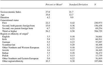
Descriptive statistics for the microdata sample are shown in table 1. Mean SEI of men in this sample is 27.0, with a large dispersion. The mean age is about 36, and the mean duration in the United States for immigrant men is about four years. About 44 percent of the men in the sample are either immigrants or the children of immigrants. Just more than 2 in 10 men (22.0 percent) have Northern or Western European heritage, while only 1.6 percent are identifiable as Jewish and 5.0 percent are Italian or Polish.
Descriptive statistics for microdata, 1900–1930 censuses.

Source: Integrated Public-Use Microdata Series 1% Sample of 1900, 1910, 1920, and 1930 censuses.
Note: Whites ages 15 to 64 who have a valid Duncan's SEI score.
a Unweighted.
b The remainder is third or higher generation, for whom we cannot track ethnic heritage. Overall N = 1,041,394.
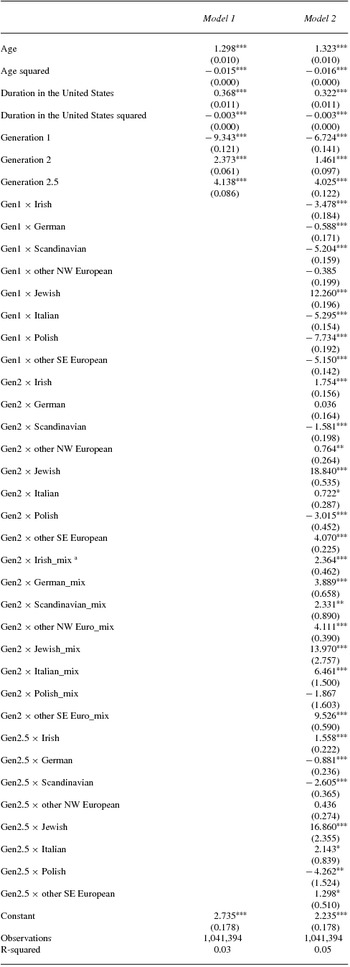
Model 1 of table 2 predicts socioeconomic outcomes for simple covariates of age, duration, and generation. These models pool the 1900–30 censuses and include white males in their labor market years. All coefficients in this pooled census sample are highly significant with p-values under 0.001. We find that age strongly predicts labor market achievement as indexed by SEI score.Footnote 10 This is in keeping with the bulk of prior labor market studies (irrespective of era and outcome measure), and so lends further confidence to using the SEI index to track labor market outcomes in the Ellis Island era. SEI rises sharply with age but at a decreasing rate, also in keeping with most labor market studies predicting socioeconomic outcomes. Our model indicates that SEI would be predicted to peak at age 43. At age 30 the slope of SEI is rising (at a decreasing rate) at about 0.8 points per year.
Individual-level microdata OLS regression results—pooled across four censuses.

Source: Integrated Public-Use Microdata Series 1% Sample of 1900, 1910, 1920, and 1930 censuses.
Note: i indexes the individual. Standard errors in parentheses. Results unweighted. Reference category for generational status variables is generation 3+. Reference category for generation × ethnicity interactions is a combination of generation 3+, English, and other white ethnic groups.
a _mix means exogamous marriage.
*** p ≤ .001. ** p ≤ .01. * p ≤ .05.
Duration in the United States (among immigrant men) is also strongly and nonlinearly related to occupational status. The SEI index is predicted to rise with time, and as with age, to do so at a declining rate. The duration slope is predicted to be 0.368 initially (duration = 0 years) and decline only modestly to about 0.308 after 10 years.
Model 1 predicts that immigrants (first-generation white men and net of duration) would score more than nine SEI points below established (third- or higher generation) white men of the same age during this era. This is quite a sharp differential, about 40 percent of a standard deviation, in outcomes. The generational or immigrant penalty appears to reverse for the second generation. Native men born of two immigrant parents hold a 2.4-unit advantage in SEI from age-mates in the established population. For men who have one immigrant parent and one US-born parent (classified here as the 2.5 generation) the advantage is even stronger. Taken together, these first results strongly suggest that much of the immigrant deficit—whether driven by lack of skills, limited acculturation, or discrimination—is erased within a generation, at least among white males in the labor force ages. This trend is visible for the total population and the metro-only population (the latter not shown).
In model 2 we keep measures of age, duration, and generational status, and we add several covariates that capture interactions among generation and the several origin groups. Model 2 captures the variation across first-generation European origins, and formal tests (versus the null of zero) indicate the greater or lesser decrement from the overall (now residual) first-generation effects. Taken together, of course, these several origin-specific coefficients are statistically significant. Italians and Poles, along with other Southern and Eastern Europeans, pay an additional penalty of five to eight SEI points beyond that of (gen1) immigrant status (a seven-point deficit). Jews, by contrast, record a higher SEI than one would expect among immigrants, and in fact have a 5.5-point advantage [12.26 + (-6.72)]. The negative offset for Germans and other Northern or Western immigrants is modest. Circumstances for Irish immigrants are intermediate, but the Scandinavians experience a deficit in magnitude of that faced by Italians and other Southern and Eastern European immigrants—about five points.
Second-generation origin effects are modest in model 2. Among those with both parents of the same origin, only second-generation Poles exhibit an added deficit (beyond the 1.46 SEI points attributable to generational status) over three SEI points. For several groups (Irish, other Northern and Western European, Italian, and other Southern and Eastern European) the offset has turned positive. For the eight distinct origin groups, we enter another set of dummy variables for whether the person is of mixed parentage, taking father's origin as the leading identifier. In none of these cases is there any further negative offset from the second-generation effect.
In a final set of comparisons in model 2, we examine working-age males of mixed-generation parentage (the 2.5 generation, one parent US-born), and identify the individual by that of the foreign-born parent's origin. Most of these are in line with the ethnic-specific effects of the endogamous second-generation results mentioned previously.
Taken as a whole, these origin-specific analyses are in keeping with the nonspecific results of model 1. Here we see a sharp improvement (decline in deficit compared to those in the established third generation) for the second generation over the first. Notably, this holds within each ethnic group, with generational improvement manifest in all, although varying somewhat by origin. Some modest variations can be observed for individuals who are of exogamous parentage. Recall that not all origin groups can be defined for all years in the table 2 regressions, so some of these results may reflect differences in identifiable composition across decades, something that can be examined more closely with separate regressions for each decade, 1900 through 1930.
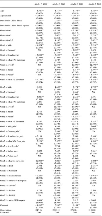
Table 3 presents companion results to those of table 2, model 2, but in which we estimate separate models for each census year 1900 through 1930. This allows us to examine the variation in predictive traits—duration, generation, and national origin—through key early decades of the twentieth century. (These models also allow the effect of age and duration—two key labor force predictors of SEI—to vary across these four census decades.) Results of this model exhibit many parallels with those of table 2, but there are also a few aspects in which the pooled results are not simply replicated across the four decade-specific regressions.
Individual-level microdata OLS regression results—split by census year.

Source: Integrated Public-Use Microdata Series 1% Sample of 1900, 1910, 1920, and 1930 censuses.
Note: i indexes the individual. Standard errors in parentheses. Results unweighted. Reference category for generational status variables is generation 3+. Reference category for generation × ethnicity interactions is a combination of generation 3+, English, and other white ethnic groups. NA means not available in that census year.
a _mix means exogamous marriage.
b The first-generation German, Jewish, and Polish are not identified in the 1900 census because mother tongue is not available that year, but they are identifiable in the other three censuses. Parents’ mother tongue is available in the 1910 and 1920 censuses only, so generation 2, 2_mix, and 2.5 × origin interaction effects cannot be discerned in the 1900 and 1930 models. As a sensitivity check, we use region-of-origin variables that are based solely on birthplace in the regression models so the groups are consistent across the censuses. Results for other covariates were broadly consistent, and we note differences between the coefficients for region of origin using these two measurement schemes.
*** p ≤ .001. ** p ≤ .01. * p ≤ .05.
All four models exhibit broadly similar coefficients for age and its square, and thus SEI improvement would trace similar patterns with age across the four census decades. More specifically, we find that the age of maximum status attainment is predicted to be in the early forties in all four years. We also find a modest increase from decade to decade in the slope of the age-attainment function when evaluated at age 30, suggesting greater early life returns to experience, itself perhaps a function of increasing education across the decades.
Duration (including its square) traces similar patterns from 1900 to 1920. In all three of these census years, one predicts an appreciable socioeconomic return to each year of US residence for immigrants. This return, while remaining positive, declines modestly with further length of stay in the United States. In 1930, however, the model deviates: both linear and quadratic terms are positive. While seemingly anomalous, the result is also intriguing. By 1930 the United States had seen the imposition of new restrictive immigration policies through the 1924 Naturalization Act (and related policies), and the start of the Great Depression. While both linear and quadratic coefficients for 1930 are positive, substantive examination indicates that the net effect is modest in size and traces a flatter trajectory.Footnote 11 For instance, in 1910 the combined duration effects predict a net increment to SEI of 4.37 points with 10 years of US experience and an increment of 10.0 SEI points with 30 years of experience (after adjustment for other controls in the 1910 model). For 1930, the corresponding SEI increments are 0.4 at 10 years and 3.0 at 30 years (with other traits controlled)—a much less pronounced duration trajectory.
These split sample results recapitulate the earlier finding of a significant deficit in predicted SEI among immigrants (generation 1), and we now observe some variation across decades. In regressions that include generation dummies but not national origin indicators (results not shown), we find that immigrants (net of age and duration, which work to improve SEI) experience SEI deficits of about five to nearly 11 points in the aggregate. Table 3 indicates the variation in national origin outcomes by generation and decade. Most of these are in keeping with the deviations we identified in the pooled results (table 2), but now we can observe deviations across the census years. For instance, immigrants from Ireland experience an SEI deficit of about eight points in 1900, while those from Italy exhibit a similar deficit. By 1930 the Irish immigrant deficit had been cut to six points, while the Italian deficit (following substantial waves of Southern and Eastern European immigrants in the interim) had grown to more than 10 points. The more recently arrived Polish and “Other” Southern and Eastern European groups also show larger offsets than the Irish in the latter two decades. Throughout the 1910–30 years (with distinct identification not possible in 1900) Jews manifest large positive offsets from other first-generation origin groups in the magnitude of 11 to 12.6 SEI points.Footnote 12
Second-generation individuals manifest SEI scores that exceed those of the corresponding first-generation group in every comparison. A simple comparison is to look at the offsets indicated by the generation-origin dummies. These offsets are net of the overall generation dummy, which in all cases favors the later generation. The implicit comparison here also sets the duration variable to zero for the first generation, thus, a new arrival. Still these comparisons do provide a useful indicator of the direction of change across generations; moreover, they provide clearer indications of the group-specific differences that exist within census decade and generation.
The cases of the Irish and Polish, as older and newer groups, respectively, are illustrative. Those second-generation Irish individuals with both parents also born in Ireland cut sharply the deficit from those in the first generation. In 1900 this second-generation group is predicted to score about 11 points higher on SEI than their first-generation conationals. The advantage is maintained through the following three decades. Second-generation Poles (of Polish-only parentage) in 1910 and 1920 appear to exhibit about a 13- to 14-point advantage over their first-generation Polish counterparts. Note, however, that the second generation of Polish parentage still falls behind their other Northern and Western, and Southern and Eastern, European peers. By 1930 those of second-generation Italian-only parentage exhibit an SEI advantage of more than 10 points over the immigrant generation.
The SEI advantage we observed for Jews in the pooled regressions is manifest in each of the separate census year regressions as well, except 1900, for which we cannot determine Jewish identity. Within the first generation the advantage over the established, English, and other ethnic white men is on the order of three to eight SEI points, and in the second generation—no matter the parentage combination—the advantage is on the order of 8.8 to 23.7 points. Second-generation Poles (of various parentage combinations) appear to be less well situated in the labor market than some other groups, although modest sample sizes of these groups caution against overly strong interpretations of any single coefficient.
These results are broadly consistent with classical assimilation theory, as described at the outset. The pooled and decade-specific regressions clearly point to positive effects of duration and generation in predicting the socioeconomic position of immigrant men and their descendants. One might consider there to be some evidence of “bumpiness” as well, if one takes differentials across ethnic/origin/generation interactions as evidence of lack of a universally smooth labor force trajectory. We now trace cohorts across censuses to see whether the view with such restructured data also confirms this picture.
Double Cohort Results
We collapsed SEI scores by specific origin-arrival-age combinations, for each census, to obtain the mean SEI for each respective group. An example of a “cohort” is Southern or Eastern Europeans who arrived to the United States between 1880 and 1899 and were 15 to 24 years old as of the 1900 census. As for the microdata analysis, this section is restricted to white men ages 15 to 64.
Cohort trajectories
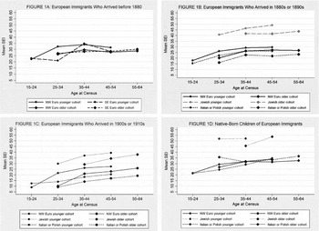
Figure 1 graphically depicts the double cohort method using the censuses from 1900 through 1930. Figure 1A displays the SEI trajectories for European immigrants who arrived before 1880 (the “prepeak” years), and we offer more detail on this graphic to indicate the general approach. Each line is the SEI trajectory across the life cycle (age) for a specific combined region/ethnic group and birth cohort. Two birth cohorts are depicted: a “younger” cohort ages 15 to 24 in 1900, and an “older” cohort ages 25 to 34 in 1900. The four points on each line represent the mean SEI score for the specific origin/age/arrival cohort. For example, looking at the line (with circle marker) for the Northern and Western Europeans for the younger birth cohort ages 15 to 24 years old in 1900 (thus born in 1875 to 1885), we see that their mean SEI was about 21 in 1900; 10 years later in 1910 when they were 25 to 34 years old, their mean SEI was about 33; by 1920 when they were 35 to 44 years old, their mean SEI rose to 34; and by 1930 when they were 45 to 54 years old, their mean SEI was about 31. A second line (with diamond marker) for Northern and Western Europeans begins at age 25 to 34 in the 1900 census (thus born in 1865 to 1875) and proceeds through the three subsequent censuses to the point when the group was 55 to 64 years old by the 1930 census. This older cohort exhibits a flatter trajectory. Successive figures 1B, 1C, and 1D apply this approach to European immigrants who arrived in the 1880s or 1890s (figure 1B—the early peak years); the trajectories of those who arrived in the 1900s or 1910s (figure 1C—the late peak); and the trajectories for the US-born children of European immigrants (figure 1D).
Socioeconomic trajectories between 1900 and 1930. Figures 1A – 1C show the trajectories for immigrants who arrived in the pre-peak, early peak, and late peak years, respectively. Figure 1D shows the trajectory for the native-born children of immigrants.

A detailed analysis (not shown) where we broke down the Northern and Western European group into its constituent ethnicities (English, Irish, German, and Scandinavian) showed that the aggregated Northern and Western European trend adequately represents each ethnicity.Footnote 13 Figure 1A aggregates the Southern and Eastern European immigrants because too few arrived during the prepeak years to disaggregate Jews from Italians and Poles. Figures 1B and 1C break the Southern and Eastern European group down into Jews, on the one hand, and Italians and Poles, on the other. The trajectories for Jews are not as long as the other groups’ trajectories in figures 1B–1D because we do not have information (mother tongue) that would enable us to identify Jewish origin in the 1900 census (for generation 1) or the 1930 census (for generation 2).
Across all arrival cohorts, the graphs depict the expected curvilinear trend of SEI increasing then leveling off with time. Figure 1A—which depicts the prepeak arrivals—shows that SEI increases for both Northern and Western European birth cohorts, and then either decreases or is stagnant when the cohort reaches the oldest labor force ages. SEI progression for the younger Southern and Eastern European birth cohort shows that they dropped but then made up the difference and caught up to the Northern and Western European younger birth cohort.Footnote 14 Otherwise, there is no major difference in these two European groups’ SEI progression across the four censuses—the trajectories for the Northern and Western and Southern and Eastern European groups who arrived before 1880 are remarkably similar. Note also that the younger Northern and Western European birth cohort ends up slightly higher than the older birth cohort on the Y-axis.
Turning next to the early peak arrival cohort in figure 1B, we see the importance of disaggregating the Southern and Eastern European group into the Jews versus Italians and Poles. Again, all groups experience upward SEI progression. Here, though, the Northern and Western Europeans are slightly lower on the Y-axis than the prepeak Northern and Western European group. As expected, we see much higher SEI scores for both Jewish birth cohorts, who surpass the Italians and Poles and the Northern and Western Europeans. The Jews’ SEI scores were likely driving what we saw in the prepeak Southern and Eastern European trajectories (similar trajectories as for the Northern and Western European group) because the Italian and Polish SEI trajectories for the early peak arrival cohort in figure 1B are consistently about five points lower than the Northern and Western European trajectories across the four decades. (See appendix A for further discussion of the Jewish population and SEI scores.Footnote 15 )
Turning to the late peak arrival cohort in figure 1C, all the trajectories are noticeably lower on the Y-axis than those of earlier arrival cohorts. While all groups experience upward SEI progression like the two earlier arrival cohorts, they each start off at much lower levels and end up (by 1930) about five points lower. Still, the Jewish population sits highest on the Y-axis while the Italian and Polish populations sit lowest.
Figure 1D shows the socioeconomic trajectories of the European second generation. Interestingly, the second-generation Northern and Western European cohorts are only modestly higher in socioeconomic attainment than the first-generation prepeak Northern and Western European group. Perhaps most noteworthy, the cohort trajectories for the second generation of Italian and Polish trajectory is not substantially lower than that of the Northern and Western European group, unlike the case for the first generation.Footnote 16
Overall, the upward trajectories with time in the labor force displayed in all four graphs support classical assimilation theory's prediction that SEI improves with time in the host society. Arrival cohort also differentially impacts SEI progression. We observe that—when looking at socioeconomic attainment across the same four census years—subsequent arrival cohorts do worse. We therefore expect a negative coefficient for the early peak and late peak arrival cohorts compared to the prepeak arrival cohorts in the aggregated regression models discussed next. The more established Northern and Western European group does not appear to derive an overwhelming advantage in SEI progression, somewhat contrary to expectation based on classical assimilation theory. For neither arrival cohort do the Italians and Poles—or the Northern or Western Europeans—ever reach the SEI achieved by the Jews. Undoubtedly still, for many individual immigrants, the US outcome represented an improvement over life expectations in the origin country.
Cohort regressions
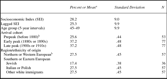
The variables used in the double cohort regression analysis are summarized in table 4. The mean SEI score for all the cohorts is 28.2 (with a minimum of six and a maximum of 68). Lagged SEI scores represent SEI the decade before. The mean lagged SEI is slightly less at 25.3 (with a minimum of four and a maximum of 60). As expected, more cohorts arrived in the early peak and late peak years (77 cohorts for each) than in the prepeak years (53 cohorts). Just more than a quarter of the cohorts are represented by immigrants from Northern or Western Europe (27.5 percent). Seventeen percent of the individuals are Jews and about a quarter are made up of either Italians or Poles. An additional quarter of the white immigrants in the analysis are from all other world regions. The mean age across the cohorts is the late forties.
Description of cohorts.

Source: Integrated Public-Use Microdata Series 1% Sample of 1900, 1910, 1920, and 1930 censuses.
Note: i indexes the cohort. N cohorts = 207.
a Unweighted.
b Reference category in multivariate regressions.
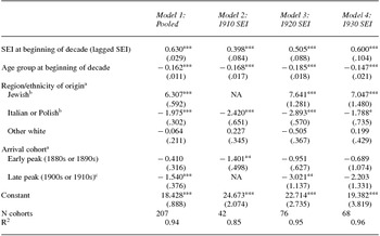
The aggregated cohort regression results presented in table 5 corroborate the patterns seen in figure 1. First looking at the effect of a cohort's lagged mean SEI on its SEI in 1910, 1920, and 1930 (the lagged SEI is from 1900, 1910, or 1920, respectively), we see in the pooled results a positive and highly significant association. That is, for any cohort, each single SEI point higher in the previous decade translates into 0.6 of a point higher SEI in the current decade, holding the other variables constant. Most likely regression to the mean effects is operating here, and hence the lagged SEI coefficient takes on a value less than unity. The pooled results have the further complication that we are pooling across pairs of census years with different age/arrival cohorts and numbers of cohorts contributed per decade. Subsequent columns show the regression results separately for each concluding census year; for example, column 4 presents coefficients for the regression of 1920 cohort-specific SEI on its corresponding value in 1910 and the other cohort covariates. These results provide the more specific manifestation of immigrant socioeconomic advancement.
Aggregated cohort-level OLS regression results.

Source: Integrated Public-Use Microdata Series 1% Sample of 1900, 1910, 1920, and 1930 censuses.
Note: i indexes the cohort. Standard errors in parentheses. NA means not available in that census year. Results are weighted by cohort size at the beginning of the decade. We alternatively weighted the results by cohort size at the end of the decade and obtained consistent results.
a Reference categories are Northern and Western European for region/ethnicity of origin and prepeak for arrival cohort.
b The German, Jewish, and Polish are not identified in the 1900 census because mother tongue is not available that year, but they are identifiable in the other three censuses. This means we do not have a lagged SEI score for the Jewish in the 1910 model. Correspondingly, the Italian/Polish coefficient in the 1910 model actually represents only Italians. As a sensitivity check, we use region-of-origin variables that are based solely on birthplace in the regression model so the groups are consistent across the censuses, and we note differences below using these two measurement schemes.
c The late peak arrival cohort is excluded from the 1910 model because this model would include only individuals who arrived between 1900 and 1919 (the late peak period) and had an SEI for 1900 (the lagged SEI score for the previous decade). Individuals who arrived between 1901 and 1919 will not have an SEI for 1900, so the only individuals included in this late peak variable in the 1910 regression model are those who arrived in 1900 and have an SEI recorded for 1900 – a small number.
*** p ≤ .001. ** p ≤ .01. * p ≤ .05.
The age coefficients display a negative relationship between age and socioeconomic attainment in each column, where SEI decreases with age of the cohort at the start of the decade. This is expected, as it reflects the curvilinear relationship between age and socioeconomic attainment seen in figure 1 and the cross-sectional regressions.
Very strong origin effects are discerned. Jewish immigrants outpace their Northern and Western European counterparts (the omitted reference category). Cohorts of Jewish immigrants are predicted to score about seven points higher SEI than Northern and Western European cohorts by 1920 and 1930, holding age and arrival cohort constant. The Italian and Polish origin groups, by contrast, exhibit a deficit with respect to their Northern and Western European counterparts in every decade. For example, Italian or Polish immigrant cohorts are predicted to score nearly three points lower SEI than those from Northern and Western European cohorts by 1920, net of age and arrival cohort. Other white immigrants do not diverge significantly from the Northern and Western European groups. This variation in outcome across the several origin cohorts may be linked directly to variations in human capital upon arrival, with Northern and Western Europeans having an advantage over some (perhaps Italians and Poles) and a disadvantage with respect to others (perhaps Jews).Footnote 17
Consistent with the double cohort graphs, we see in this multivariate framework that cohorts arriving later in the Ellis Island era (“early peak” and “late peak”) exhibit generally lower socioeconomic outcomes than the reference group of pre-1880 arrivals once age and region/ethnicity are controlled. The pooled results show that on average, immigrants who arrived most recently gained less in SEI across the censuses than peers of earlier vintage. Such findings as these may reflect better skill endowments among the earliest arrivals (the “prepeak” cohorts). Being the newest arrivals in the host society may not have specific disadvantages; rather, earlier immigrants may have been more positively selected at their origin. By 1930, where we do not see a significant difference compared to prepeak arrivals, immigration was abating and legal restrictions on immigration had already begun to be enforced.Footnote 18
Conclusion
The Ellis Island narrative continues to hold significant sway over the story of the immigrant experience in the United States. To be sure, those who came to America's shores in the late nineteenth century and early twentieth century found, on balance, success in their new land. Much has been written to document this assimilation. At the same time, questions linger empirically regarding the uniformity and rapidity of that assimilation. This is all the more so, and more importantly so, as twenty-first-century writing about twentieth-century immigration criticizes and questions the universality and “straight-line” nature of assimilation, even as it employs the Ellis Island era as the benchmark or the canonical experience of adjustment following international migration.
We exploited the richness of historical census microdata to begin to photograph statistically the Ellis Island era in greater resolution. Just as the greater accessibility of photography provided more accurate pictures of the new arrivals and their early US lives, so too these early decennial census data files provide a more accurate picture of the assimilation experience: what was common across groups and what was not. We approached this task with a two-pronged method. In one line of work, we considered each census separately and cross-sectionally, exploiting the full microdata sample at the individual level. In doing so, we conducted cross-sectional regressions on socioeconomic attainment (using Duncan's SEI index as the outcome) and predicted socioeconomic standing as a function of age, duration in the United States, generation, and region of origin. In this approach, we were particularly interested in examining the progression of origin groups across generations. In the second prong, we aggregated the IPUMS decennial census microdata into double cohorts, groupings of individuals by age and period of arrival that could be aligned across subsequent decades. These give trajectories for the underlying cohorts, although (as samples) the data are not for the very same individuals.
Our results buttress some conventional scholarly viewpoints on immigration, but they also serve to potentially reposition some thinking. (We acknowledge that viewpoints are not all in consensus and surely have changed themselves over the decades!) On balance we find both continuity and progress from decade to decade. Our simple summary graphics point to SEI improvement for most groups across most decades. We also see a slowing of the rate of progress within one's working life as time wears on, not surprising for those familiar with labor market studies. At the same time we detect appreciable differences by region of origin (ethnicity) in both our cross-sectional and double cohort models. Jews of each generation (identified from language information, following prior scholarship) achieve higher scores than other groups. Italian and Poles of each generation—merged here as major representatives of the “new” immigration—do less well than the reference group of immigrants from Northern and Western Europe. Finally, although it pushes the limits of our data, our cohort models also detect some variation by vintage, as immigrants arriving during the “late peak” period, that is, 1900s and 1910s, fare somewhat less well.
The cross-sectional microdata regressions provide important additional insights regarding the Ellis Island era and the assimilation experience during the early twentieth century. Our regression equations confirm the expected gains in socioeconomic attainment that come with labor market experience (age) and duration in the United States. At the same time we see appreciable generational advance, arguably larger than that often anticipated by writers of the Ellis Island era or those more recent scholars looking back on the era. For working-age white males, time clearly bestows benefits: we observe appreciable gains over time among the immigrants in their own working years and then across the generations. Such results complement the findings of the double cohort analyses. We do also find some deviations from any all-encompassing model of assimilation and inclusion. While our results are bound by the necessary limitation of working with historical census data, we appear also to be able to detect a widening regional (ethnic) gap by 1930. One possible explanation is that the concern seen in the national immigration discourse, particularly voiced with reference to new arrivals from Southern and Eastern Europe, is also translated into the context of reception in the labor market and an ensuing penalty in SEI scores that we detect. Future research along these lines, perhaps exploiting regional variation in policies, could shed light on this.
Although these census data do not allow us to test possible mechanisms, we can speculate about what might have been driving the observed results. Human capital characteristics were surely at play. English-language facility clearly provided advantages for immigrants from English-speaking countries, while Italian and Polish immigrants were set back by having to learn a new language. However, neighborhood enclaves and workplace niches likely allowed non-English-speaking immigrants to find jobs and navigate through their new host society. Jewish immigrants are an example of newcomers who did not speak English upon arrival yet flourished in their host economy. Jews have historically been highly educated, skilled, and entrepreneurial, thus placing them at a higher starting point on the socioeconomic hierarchy and buttressing their socioeconomic progress. Italians and Poles who entered the United States during the Ellis Island era tended to have little education and were less likely to be trained in highly skilled trades. Educational attainment was much higher for second-generation Italians and Poles in the United States and surely contributed to their catch-up in terms of SEI scores. These second-generation individuals may have benefitted particularly from the comparatively strong US investments in education during this period (Garfinkel et al. Reference Garfinkel, Rainwater and Smeeding2010). The second generation also learned English in school, providing more avenues for socioeconomic gain. Changes in household composition may have played a role in promoting intergenerational socioeconomic progress. Immigrants from Northern and Western Europe had lower fertility rates at the end of the nineteenth century than immigrants from Southern and Eastern Europe (Morgan et al. Reference Morgan, Susan Cotts, Douglas and Cotts Watkins1994), and second-generation adults had fewer children than their immigrant parents (King and Ruggles Reference King and Ruggles1990), perhaps resulting in greater investments in each child's education for those groups. Fewer children may have been working in family businesses at a young age and leaving school early to run the business.
As for the lower predicted SEI scores for the latest arrival cohort (those who arrived in the “late-peak” years 1900 through 1919), this may be related to saturation effects stemming from the oversupply of labor, or perhaps to a less welcoming context of reception as public opinion toward immigrants turned more negative, as manifest in restrictive policies of the 1920s. These individuals arrived toward the end of the great wave of immigration and were perhaps at a disadvantage in finding jobs that would allow them to climb the socioeconomic hierarchy. The Great Depression may have hit these late arrivals harder also, if they already had less job security from having been in the United States for less time and were working in jobs more prone to economic fluctuation, such as construction and service.
Taken together, our empirical analyses of these historical census data highlight immigrant and second-generation success in the Ellis Island era. Gains were broad-based across origin groups and period of arrival. Most striking in our findings, perhaps, is the marked weakening of such socioeconomic attainment differentials already by the second generation. Not all was equivalent, however. A uniformly operating US assimilation machine would have made no room for explanatory power due to ethnic origin or period of arrival, and we find evidence for both. Some of these differences are, no doubt, attributable to differences in skills brought with them by immigrants to Ellis Island and other US ports of entry. But we may also be observing in these results the rise in differential treatment visited upon new arrivals, a differential reception that would become manifest in growing doubt about assimilability and ensuing restrictions on immigration by the end of the Ellis Island period.
While our results remain only as refined as census data allow, they do point to a more rapid assimilation than many observers of the period allowed. Historian Woodham-Smith's (Reference Woodham-Smith1962: 203) concern that it would take “until the second or third generation” may have been more guarded than necessary and the Dillingham Commission's views more pessimistic than justified. Such progress about a century ago may, in turn, suggest that we reflect again on our theories of immigrant incorporation and the likely progress of new arrivals in the present era.
Appendices
Appendix A: Methodological Appendix
Census Data
While IPUMS census data confer the advantage of synthesizing panel data, these historical data also present some challenges. First among these challenges is the issue of population change across censuses. Our aim in this analysis is to tap the same pool of people across the censuses, yet we acknowledge that when we combine several censuses into one large population, we end up with a meta-population, so to speak, because the data set no longer represents a snapshot of the population from one year. The population changes depending on, for example, subgroup coverage, how people identify themselves in terms of ancestry or ethnicity, and emigration from the United States.
A second challenge is the work norms at the turn of the twentieth century. The labor force universe in these censuses is individuals ages 16 or older. We have occupations recorded for individuals younger than 16 because the occupation universe is those ages 10 or older in the 1900 census, and all persons in the 1910, 1920, and 1930 censuses. Census enumerators were instructed to record an occupation for any person “gainfully employed”—a somewhat ambiguous term when applied to children. These individuals are likely working for their parents, not independently (Minnesota Population Center 2011), so any observed SEI change for them would be partly a product of their working with their parents. We choose to include individuals ages 15 to 64 to be consistent with other literature covering the same era, and because individuals commonly began working in their early teens in the nineteenth and early twentieth centuries.
Additionally, we have some degree of omitted variable bias because the census does not include all relevant variables and because of the cross-sectional nature of the census. An example of such an omitted variable is educational attainment, which was not asked of the US population until the 1940 census. Education may have been an important differentiator. Foner (Reference Foner2000) notes, based on analysis of primary documents that offered a glimpse at education at the time, that literacy made a difference at the turn of the twentieth century. One quarter of Jews, versus one half of Italians, told immigration officials upon entry at Ellis Island between 1899 and 1910 that they were illiterate. Italian children had lower school enrollment rates than Jewish children, and they were likelier to drop out of school before the minimum grade requirement (ibid.). However, Foner also comments that businesses, not education per se, were the vehicle for Jews’ occupational advancement during the Ellis Island era. Only starting in the 1920s and more so in the 1930s did their children use secondary and tertiary education to advance occupationally (ibid.). Still, low overall education levels at the time, ceiling effects for education, and unequal effects of education on occupational status for minorities (Tolnay and Eichenlaub Reference Tolnay and Eichenlaub2007) might be the reason why we do not observe steeper SEI trajectories in figure 1.
Occupational Coding and SEI Scores
As we demonstrate in this study, Jews exhibit dramatically higher average SEI scores than all their peers during this period. Inspection of SEI quartiles illustrates how the Jewish population is set apart (and above) other men in the sample. The 25th percentiles for Jewish men, Italian or Polish men, and Northern and Western European men, respectively, are 18, 8, and 10. This means that among white men ages 15 to 64 who are in the labor force, 25 percent of Jewish men have an SEI score of 18 or lower, 25 percent of Italian or Polish men have an SEI score of 8 or lower, and 25 percent of Northern and Western European men have an SEI score of 10 or lower. For the 50th percentile, the corresponding numbers are 27, 12, and 18. For the 75th percentile, they are 68, 19, and 34.
Of concern to us is whether the Jewish population's more favorable SEI distribution is a product of the way occupations were coded and ranked when Duncan constructed the SEI scores. A higher proportion of Jews are concentrated in occupations that correspond to higher SEI scores. For example, 22 percent of Jews were managers and officials at the time, compared to only 2 percent of non-Jews. We also observe that Jews worked in industries comprised of higher SEI occupations. We do not know, however, what kinds of management and official positions these are, for example, exactly what skill level is involved.
Emigration
While estimates of emigration are likely underestimates because of poor data quality (King Reference King1978; Warren and Kraly Reference Warren and Ellen Percy Kraly1985; Wyman Reference Wyman1993), many historical demographers have dug through available secondary sources to provide some context of emigration during the Ellis Island era. During the twentieth century, the estimated ratio of immigration to emigration was 3:1 (Warren and Kraly Reference Warren and Ellen Percy Kraly1985). Between 1880 and 1930 specifically, an estimated one-quarter to one-third of all European immigrants to the United States returned to their origin country, translating to about 4 million persons (Wyman Reference Wyman1993). Other demographers report that 4 million immigrants exited the United States between 1900 and World War I alone (Warren and Kraly Reference Warren and Ellen Percy Kraly1985). Italians were the most active return migrants: about 30 to 40 percent of Italians returned to their native country, compared to 10 percent of Irish immigrants (Wyman Reference Wyman1993). Cinel (Reference Cinel1991) estimates 48 returns to Italy for every 100 departures between 1902 and 1910.
Emigration to the United States was an earnings strategy for investing back in the origin country after laboring abroad, and trips to the United States were intended to be of short duration—a means rather than an end. Immigrants attained their target savings and returned home (Cinel Reference Cinel1991; Wyman Reference Wyman1993). Cerase (Reference Cerase1974: 251) calls this “returns of conservatism”; some of those who succeeded in the United States returned home because they always intended to return home, not because they were unsuccessful. According to Cinel (Reference Cinel1991), many returnees resettled back in the United States because they were unsuccessful at investing the money they earned abroad back in their origin country, or they reemigrated in order to continue to earn money (Cerase Reference Cerase1974). One study of Hungarians found that those who “failed” were actually less likely to return home due to shame (Wyman Reference Wyman1993).
The nature of jobs available to immigrants in the United States facilitated circular migration. For example, many Italians in New York and across the United States worked in construction, which halted during the winter months; during these months immigrants returned home because doing so was cheaper than staying in the United States until the trade resumed in the spring (Cinel Reference Cinel1991).
Some studies of more contemporary emigration discount the severity of a negative economic selection bias. Gmelch's (Reference Gmelch1983) study of Irish and Newfoundland return migrants in the late 1970s found that “patriotic-social” and “familial-personal” pull factors (respectively, identification with the origin society and desire to live near kin) outweighed “economic-occupational” pull and push factors (respectively, job or business opportunities at home, and being unemployed or disliking one's job) (Gmelch Reference Gmelch1983). Although Constant and Massey (Reference Constant and Douglas2003) document that emigrants leaving Germany in 1984 are negatively selected with respect to occupational prestige, the authors show that stayers’ earnings are not biased by this selective emigration.
In our census-based samples, we attempted to assess the extent to which attrition impacts our sample by tracking age (birth) cohorts across the four censuses in a Lexis diagram, by region of origin (not shown). The degree of emigration can be elusive in census data because, although many people may leave the United States, many people may enter the United States, balancing out losses and rendering them unobservable. Changing census procedures and collection dates can impact the numbers also. For example, immigrants may arrive in the United States in 1900 but after the census was taken, thereby not showing up in the 1900 census, but they will show up in the 1910 census if they remained in the United States. This would present an erroneous spike in the number of immigrants arriving between 1900 and 1910. Further, the benchmark for “usual place of residence” in the four censuses differed; they were June 1, April 15, January 1, and April 1, respectively. Our own examination suggests that attrition appears highest among the oldest persons (ages 55 to 64) between 1910 and 1920, and between 1920 and 1930. Greater returns among older age groups are expected, reflecting returns for retirement and target earners reaching their earnings goals. The dramatic drop in Southern and Eastern European immigrants between 1920 and 1930 reflects the 1924 National Origins Act, which restricted the immigration quotas for Southern and Eastern Europe.