Latin America has been famous for its historically unequal distribution of income and wealth. In the past 20 years, scholars have argued that the origins of Latin American development and inequality are rooted in the initial endowments faced by settlers in the colonial era (Acemoglu, Johnson, and Robinson 2001, 2002; Deininger and Olinto 1999; Dell 2010; Engerman and Sokoloff 1997, 2000, 2002, 2004; Easterly 2002, 2007; Easterly and Levine 2003; Galor, Moav, and Vollrath 2009). These “endowment theories” state that initial endowments shaped institutions in the new colonies. These institutions then persisted over time and explain a great deal about economic outcomes in the present. For example, Stanley Engerman and Kenneth Sokoloff claim climate and soil conditions were suitable for different crops in the new colonies, and the differences in the economic structure of different types of crops led to distinct differences in the concentration of wealth and institutions across Latin American countries. These initial conditions favored institutions that perpetuated inequality over time. D. Acemoglu, S. Johnson, and J. Robinson also track inequality to colonial institutions, but identify inhospitable disease environments as the main driving force behind the colonial institutional framework. In locations where the environment was hostile to European settlement, more unequal institutions persisted. The persistence argument has been so influential that the seminal work on world inequality by F. Bourguignon and C. Morrisson (2002) assumed invariant inequality for Latin America until 1950.Footnote 1
A second view stresses transitions into and out of the global economy as major forces that influenced inequality in Latin American countries (Bulmer-Thomas 1994; Williamson 2002; Coatsworth 2005; O'Rourke, Taylor, and Williamson 1996b; Williamson 2010). As a result, they tell a story of much more diverse trajectories in economic growth and inequality across Latin American countries after they gained independence.
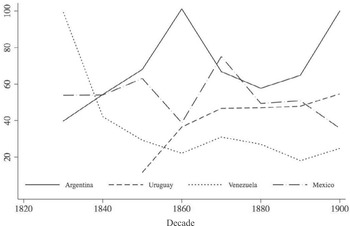
Unfortunately, much is asserted about the paths of inequality in Latin America but little is known about their actual historical evolution. Using freshly unearthed evidence, I document the changes in inequality in Argentina, Mexico, Uruguay, and Venezuela between the 1830s and the 1900s. As seen in Figure 1, the extent of inequality varied substantially across countries, and there were large fluctuations in inequality within each country over the course of the century. The fluctuations suggest that today's inequality is not simply a persistent legacy of initial colonial institutions.
During this period, the countries severed their ties from colonial rule. As the new nations struggled to achieve political unity, their economies also experienced important changes, including trade integration together with land expansion and population growth. All of these forces affected the return to factors of production, which led to fluctuations in inequality. To show the influences of these changes in factor endowments and access to trade on inequality, I develop a structural model and use it to perform counterfactual analyses. The counterfactual exercises suggest that factor endowments and trade mattered a great deal. While colonial trade was restricted in terms of goods and authorized ports, independence resulted in the expansion and the adaptation of trade and greater integration with world markets. Where the export products were land-intensive, inequality tended to increase with rising in the terms of trade. The changes in inequality also depended critically on the relative scarcity of land and labor and on the distribution of land ownership. Population growth, especially when caused by migration, increased inequality, holding other factors constant. Finally, the opening of new land on the frontier served to reduce inequality.
INEQUALITY IN FOUR LATIN AMERICAN COUNTRIES, 1820S.1900S (Argentina 1900 = 100)

DEVELOPMENT AND INEQUALITY MOVEMENTS IN FOUR COUNTRIES
To understand Latin American inequality, it is first necessary to identify the historical forces of continuity and change. The inherited colonial structure of landownership and labor supply had a substantial weight in independent Latin America. Trade was highly regulated. However, parts of the colonial legacies were challenged during and after independence. Trade integration had a particularly deep impact on the allocation of factors of production and inequality.
The colonial institutions of control over the land and the people had tangible consequences for the societal structure during independence.Footnote 2 Of particular importance were the labor practices used to guarantee provision of labor to key productive areas such as mining and agriculture. The Spanish settlers adopted and adapted labor-drafting practices already present in the New and Old Worlds. Two became the most relevant: the mita and the encomienda.Footnote 3 The mita was a temporal arrangement to supply labor to mining in Bolivia and Peru while the encomienda was used for labor provision in other economic activities. This system existed throughout colonial times; however, the extent, intensity, and prevalence varied widely across Spanish Latin America. Moreover, a continuous flow of African slaves was employed in the most dynamic crop-producing colonies in the region. The existence of slavery and labor drafting practices are of crucial importance in the dominant view on economic development in the region.
The political discontinuities experienced with the declaration of independence in each nation altered the organization of Latin America (Haring 1975; Skidmore and Smith 2001). Independence allowed for the modernization of the nation-states and further integration in the world economy (Coatsworth 1993a, 1993b). Each country experienced significant changes in population and land availability, together with ever-moving relative commodity prices. These changes were profound enough to influence inequality in the region. In this sense, the role of colonial institutions has been overstated by not taking into account the richness of the postcolonial historical experience of the region.
In particular, I concentrate on four distinct countries: Argentina, Uruguay, Venezuela, and Mexico. Mexico was a pillar in the Spanish colonial venture with a steady supply of indigenous labor and abundant silver. Argentina and Uruguay played a marginal role on the fringes of the empire with no precious metals and belligerent nomadic populations. Venezuela's experience was somewhere in the middle. From a production perspective, Argentina and Uruguay exported mainly livestock byproducts and grains, Venezuela specialized in plantations crops such as coffee and cacao, and Mexico in silver and agricultural products. In terms of factor endowments, all four countries brought tracts of land into production throughout the nineteenth century.
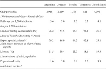
SELECTED INDICATORS, CA. 1900S

Sources:
GDP per capita: Maddison (2002). Argentina: Railroads: Vazquez-Presedo (1971). Land ownership concentration: based on Comision Directiva del Censo (1898). Export specialization: livestock byproducts as share of total exports based on Dirección General de Estadística (1916) and Vazquez-Presedo (1971). Literacy: literate share of population 14 years of age or older, based on Comision Directiva del Censo (1898) and Vazquez- Presedo (1971) Population density: from INDEC (1975). Uruguay: Railroads: Finch (2005) Land ownership concentration: based on Acevedo (1903). Export specialization: livestock byproducts exports as share of total exports, based on Bárran and Nahum (1967) and Consejo Nacional de Administracion Uruguay (1925). Literacy: literate share of population 14 years of age or older from Finch (2005). Population density: based on Consejo Nacional de Administracion Uruguay (1925) and Finch (2005). Mexico: Railroads and Land ownership concentration: based on Dirección General de Estadística (1956). Export specialization: silver and agricultural products exports as share of total exports, based on Herrera Canales (1977) and INEGI (1999). Literacy: literate share of population 12 years of age or older, based on Dirección General de Estadística (1901). Population density: from Dirección General de Estadística (1901) Venezuela: Railroads: Izard (1970). Land ownership concentration: based on Baptista (2006) and Brito Figueroa (2002) Export specialization: cacao and cofiee exports as share of total exports, based on Baptista (2006) and Izard (1970). Literacy: literate share of population 14 years of age or older, based on Junta Directiva del Censo (1891). Population density: from Junta Directiva del Censo (1891). United States: Carter et al. (2006).
Table 1 sketches some of the contrasts at the end of the century of study. Unfortunately, some of the most basic indicators of development are not available for these countries for most of the nineteenth century. The early Republican years were plagued by internal instability as the region attempted to shed its colonial legacy. However, by the turn of the twentieth century, all four countries were on an expansionary path after embracing the well-known export-led strategy. Export specialization was the rule, as the four countries’ exports were concentrated in a handful of commodities.
The differences in development are striking. In 1900 the Argentine and Uruguayan levels of GDP per capita reached 71 percent and 54 percent of the United States level, respectively, while Mexico's and Venezuela's GDP per capita only amounted to 33 percent and 20 percent (Maddison 2002). The rankings of literacy rates were roughly similar. Argentina and Uruguay had the highest literacy rates of 51.5 percent and 59.4 percent respectively. Mexico and Venezuela lagged considerably behind at 22.3 percent and 18.6 percent. The rates in all four countries were much lower than the 89 percent rate in the United States.
Much of what we know about long-term Latin American economic history has emerged fairly recently. After searching through a broad range of national archives throughout Latin America, I have compiled and constructed a new data set on wages; land, commodity, and manufacturing prices; labor force; land stock; interest rates; and a variety of export and import statistics over a long time period in the four countries.Footnote 4
An important contribution of this article is the calculation of inequality measures for four Latin American countries across more than eight decades.Footnote 5 Unlike studies on contemporary inequality that use summary indicators such as the Gini coefficient or the Theil index, my indicator is the ratio between land rent and the unskilled wage. To estimate the land rentals, I collected agricultural land prices and converted them to implied rentals by using interest rates and depreciation rates.Footnote 6
Although imperfect, this measure of inequality conveys the earning power of the wealthy relative to earnings of a large share of the working population. Historical accounts and fragmentary data support the claim that the Latin American upper class was composed largely of landowners, while most workers labored in unskilled occupations. Pioneering historical works by K. H. O'Rourke, A. M. Taylor, and J. G. Williamson (1996a), L. Bértola (2000), and O'Rourke and Williamson (2001) used the same methodology to study trends in inequality during the first globalization wave.
The rent-wage ratio can be calculated for a very long period of time and it is highly correlated with other measures of inequality when multiple measures are available for comparison. E. Anderson (2001) finds that inequality trends were similar for Australia and Canada using both the rental-wage ratio or wage inequality. L. Prados de la Escosura (2008) found the ratio to be closely correlated with Gini coefficients for Spain. The rent-wage ratio may not work as well in the modern era. Bértola, Prados de la Escosura, and Williamson (2010) warned that the importance of land in production decreases when economies transition to industrialization. However, in my sample, the economies were driven mostly by the agricultural sector. The ratio in this article literally translates as the number of full-year salaries an unskilled worker had to accumulate in order to rent a one thousand hectare plot of land for a year.Footnote 7
The geographical coverage varies by country. The prices for Argentina correspond only to the Buenos Aires province. For Uruguay, I use the mean of the regional prices as provided by J. Barran and B. Nahum (1967). The observations for Venezuela include 14 of the 20 current states. For Mexico, the data only cover a few provinces in the central region.Footnote 8 The data set compiles wages for different unskilled occupations in urban settings. Typically, these included peons, servants, and watchmen. The sources vary by location but often are accounting records of hospitals, charities, schools, and the public sector. Optimally, I would have incorporated rural salaries; however, it was fairly difficult to find consistent records for a continuous period of time.Footnote 9
Domestic and external factors had sizable impacts on inequality. To quantify their evolution, I calculated the annual stock of arable land and the total labor force by country. Land was not a fixed factor of production in this part of the world because large tracts of land were brought into production at various times. The estimation was made possible by looking at the earliest figures in censuses in the late nineteenth century and then using careful accounting of public land leases and sales to estimate stocks of land in earlier periods. The data are available in archival records of the individual countries and a few secondary publications. In estimating the labor force, I considered the losses from violence in some cases and the major gains from immigration. The calculation involved two steps: taking into account the net migration flows, as most of the immigrants were of working age, and then accounting for the age distribution of the native population at different points in time to calculate the total labor force.
To evaluate the impact of trade, terms of trade were collected from secondary sources. When these were not available, I estimated the overall terms of trade with data collected on certain prices of exports and imports and trade composition available in economic bulletins and newspapers.Footnote 10
THE INFLUENCE OF TRADE AND FACTOR ENDOWMENTS ON INEQUALITY
The breakdown of colonial power in Latin America brought about significant changes in the functioning of the economies in the region. These winds of change had material effects on inequality. In all countries, land put into production increased at varying rates, from a mere 13 percent in Venezuela to over 400 percent in the case of Argentina.Footnote 11 The increase in population was equally dramatic between 1830 and the early 1900s. Uruguay's population grew 11-fold while Mexico's nearly doubled. These movements in labor and land supplies modified the relative scarcity of land in all countries. In Uruguay, population grew much faster than the supply of land, such that the land-labor ratio fell from 78 to 29 hectares per laborer in half a century. Terms of trade were fairly volatile with large fluctuations ranging from −20 percent to +30 percent on an annual basis.
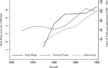
The changes in Uruguay conform to the expected movements of inequality based on profound changes in the relative factor endowments and increasing terms of trade. During the nineteenth century, Uruguay expanded the share of land under production from 11 percent to nearly 90 percent of its arable area. Even so, Uruguay was the host of significant immigration during the era of mass migration and the labor-land ratio in Figure 2 nearly tripled between 1850 and 1900. To make this case even more interesting, the terms of trade rose by nearly two-thirds between 1860 and 1890. Unlike Argentina, the agricultural sector was more developed in the early independent years. However, its growth was severely interrupted by a long-lasting struggle to control access to land. La Guerra Grande of 1839–1851 translated into a considerable loss of lives and cattle. After this internal war, Uruguay replenished its cattle stock and continued incorporating land into production, albeit at a slower rate than population growth. Immigration further accelerated the trend toward a higher labor-land ratio. The increasing labor-land ratio paired with favorable terms of trade were associated with a sharp rise in the rent-wage ratio.
URUGUAY: RENT-WAGE*, LAND-LABOR RATIOS, AND TERMS OF TRADE

Consistent with fragmentary historical evidence, the Uruguay rent-wage ratio measure of inequality rises from around 1 in 1850 to 5.5 by 1870 and then to above 6 by 1900. The trend arose even as two opposing and substantial changes in factor endowments arose in the economy. Immigration pushed inequality to increase when labor became relatively more abundant. By 1880 one out of three inhabitants of this country was foreign. The largest influx of immigrants arrived in the 1880s, which coincides with the plateau in inequality. Decreased mortality together with stable fertility rates contributed to a renewed rise in the amount of labor in the late nineteenth and early twentieth centuries. On the other hand, expansions in land under production pulled inequality in the opposite direction. The annexation of land to production ameliorated the potential climb of inequality.
Meanwhile, the existing pastoral economy was the base for the expansion of the Atlantic trade, as livestock by-products accounted for almost 90 percent of the total exports. Measured in real terms, total exports increased seven-fold from the late 1860s until 1913, the culmination of the first globalization. Advantageous terms of trade also contributed to the expansion of the export sector.Footnote 12
The Argentinean journey in the nineteenth century presents some similarities to the path followed by its neighbor. Large tracts of land were annexed, immigration expanded in the later decades, and the terms of trade were also favorable. However, the initiation to independent rule coincided with the beginnings of a more dramatic change in Argentina's participation in world trade. On the eve of independence in 1816, Argentina's main export was silver and only 20 percent of Argentinean total exports were agricultural. The transition from colonial times and the expansion of international trade led to the virtual disappearance of silver as the main export product and replaced it with livestock by-products such as jerky and hides (Newland and Poulson 1998). In the late eighteenth century, the main port of Argentina, Buenos Aires, shipped the bulk of the silver produced in Bolivia and accounted for up to 80 percent of total exports. By comparison, 98.6 percent of exports were of animal origin by mid-nineteenth century.
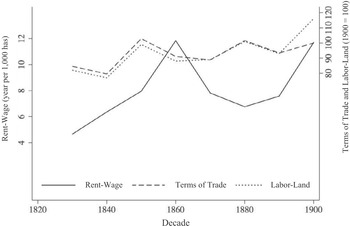
In Argentina, inequality rose between 1820 and the 1860s, then fell only to increase again in the last decades of the nineteenth century. The rent-wage ratio in Figure 3 climbed from 4 to nearly 12 from 1830 to 1860 and then dropped to 6 in two decades. This mid-century peak was driven by the wool fever that raised land prices. Later in the century, the inequality ratio increased near 12 again as more immigrants arrived and the terms of trade accelerated.Footnote 13
ARGENTINA: RENT-WAGE*, LAND-LABOR RATIOS, AND TERMS OF TRADE

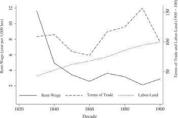
In Venezuela, roughly 12 percent of the arable land was added into production during the nineteenth century. Although Venezuela was underpopulated on the eve of independence, it failed to attract immigrants throughout the century. The inequality trajectory in this country is quite puzzling. While the terms of trade declined 30 percent, the rent-wage ratio in Figure 4 plummeted from 12 to 2. Domestic instability plagued period between the 1830s and the 1850s as frequent rebellions led to the abolition of slavery by mid-century. A rise in terms trade, on the other hand, was associated with a slight decrease in the rent-wage ratio in the 1870–1900 period.
The contributions of changes in factor endowments and terms of trade do not fully explain the trajectory of inequality in Venezuela. One reason why may be postcolonial instability that affected greatly the returns to land. Instability marked the birth of Venezuela as an independent nation.Footnote 14 The wars of independence wreaked havoc on the Venezuelan productive structure. From holding the monopoly of cacao in the Spanish Empire, the country had to rebuild itself by incorporating coffee into its production portfolio. The evidence suggests that inequality was shaped by domestic turbulence in the first decades. The integration into world markets picked up steam in the late nineteenth century as exports doubled relative to their levels in the 1860s. However, this movement coincided with a reversal in terms of trade that helped push inequality to lower levels. Moreover, the extent of land expansion paled in comparison to Argentina. While there was a definite western movement of the frontier to land better suited for coffee production, a decrease in the mortality rate propelled population growth, raising the labor-land ratio by almost 140 percent from the 1830s through 1900.Footnote 15
VENEZUELA: RENT-WAGE*, LAND-LABOR RATIOS, AND TERMS OF TRADE

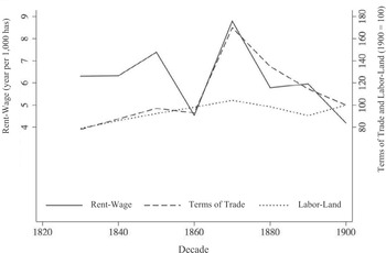
MEXICO: RENT-WAGE*, LAND-LABOR RATIOS, AND TERMS OF TRADE

Mexico was a key pillar in the Spanish colonial empire, but real GDP declined by 37 percent from 1800 to 1860, as silver production declined. Meanwhile, the inequality measure in Figure 5 rose slightly between the 1840s and 1850s, followed by a sharp decrease driven by the instability of the French intervention (1864–1867). For the rest of the century, inequality trailed the movements of the terms of trade. The rent-wage ratio rose from around 6 to 7 between the 1840s and 1850s and fell sharply to 5 in the 1860s before spiking to almost 9 a decade later. A plunge in the price of silver contributed to the large decline in the terms trade between 1870 and 1900 in Figure 5, and the rent-wage ratio fell at nearly the same pace to roughly 4. The slow rise in the land-labor ratio into the 1870s in Figure 5 put downward pressure on the wage-rent inequality measure. Between the 1870s and the 1890s the land-labor ratio fell and worked against the overall trend toward lower inequality.Footnote 16
A SIMPLE MODEL OF INEQUALITY CHANGE
The description of the changes in the four countries show that land-labor ratios, the terms of trade, and the rent-wage ratio changed at different rates across the decades. In some periods, the changes in terms of trade or the rent-wage ratio exerted pressures that were working against the changes in the actual rent-wage ratio. It is helpful therefore to develop a model that links the observed movements in the rent-wage ratio with the observed movements in labor supply, land supply, and terms of trade and better quantify the relationships in each country.
Consider a small open economy populated by dynasties and two productive sectors with imperfect domestic capital markets.Footnote 17 Each dynasty consists of two representative agents. Each lives for two periods: young and old. In this overlapping generation framework, parents are altruistic and care about the welfare of their children. They leave an inheritance and support them in their younger years.Footnote 18 Agents are under the care of the older generation when young, and work and reproduce later. Happiness is increased with higher consumption and more bequests to their offspring. Consumption takes place during adulthood as the parent provides for the basic needs during childhood.Footnote 19 Preferences are homogeneous across individuals. The utility function assigns weights to consumption, c and transfers to offspring, b.Footnote 20

where α ε (0; 1).
Each individual in a generation faces similar constraints: consumption and transfers are financed by income flows (I) in adulthood. Transfers to the younger generation are the result of savings s t+ 1 to be transferred in the form of a bequest.


In an egalitarian world, all generations display the same behavior. All individuals work during adulthood and leave part of their lifetime income to their children. In a more realistic setting, agents’ choices are restricted by the assets inherited, those accumulated, and the functioning of the markets. In particular, this economy can transfer wealth across generations through two assets: capital and land. Intergenerational transfer implies the existence of capital markets. However, domestic capital markets are imperfect in the sense that agents are constrained in the amount they can borrow based on their collateral. It is further assumed that investment in land is lumpy. The indivisibility arises from the minimum productive scale for an agricultural productive unit. As a consequence, only some individuals are able to invest in land. Society is then divided into landowners and landless workers. Therefore the distribution of wealth at a given point in time determines investment in capital and land. In nonindustrialized economies, land has a preeminent economic role. Not only does it function as a vehicle of wealth transference over time, but it also provides the possibility of acceding to financial markets that allow expansions in investment and enable consumption smoothing over time (Deininger and Feder 2001). Taking into account this feature, this stylized society has two groups classified by their ownership of assets.Footnote 21
The income of landless workers or peons (P) depends on the return on capital and labor.
![\[
\begin{array}
b_{_{t + 1} }^P = \left({1 - \alpha } \right)\left[{w_{t + 1} + \left({1 + r_{t + 1} } \right)b_t^P } \right]
\end{array}
\](https://static.cambridge.org/binary/version/id/urn:cambridge.org:id:binary:81773:20160629041142101-0619:S0022050713000028_eqn4.gif?pub-status=live)
For landowners or elites (R) land ownership and the returns to land and capital determine their income and the size of transfers to future generations.

where ρ* is the return to land and capital, and r is the exogenous return to capital.
The choices made by each of these groups converge to a unique stationary equilibrium based on their savings alternatives and returns. The lump-sum investment requirement in the land market paired with the imperfection in capital markets shape the stationary equilibrium in this economy. The membership of the two groups persists over time in the absence of shocks that can potentially induce some households to move up or down in the economic ladder.
The aggregate supply of factors of production depends on the composition of the society. The adult poor population (P) makes up the labor force (L). Capital and land are supplied depending on the saving decisions of the upper class. Given the domestic capital imperfections, the rich optimize their portfolio based on the returns to land and capital while the lower class provides labor. However, capital also flows from abroad. The fact that this economy is open allows for international capital inflows (Ke).
In the case of no population growth, the supply of factors of production is given by


where μ and 1–μ are the rich group's portfolio shares allocated to capital and land respectively.
Production takes place in two sectors: agriculture (A) and manufacturing (M). Not all factors are used in both sectors: manufacturing uses labor (L) and capital (K); whereas agriculture uses land (T), labor (L), and capital (K). Both sectors exhibit constant returns to scale.Footnote 22 The small open economy assumption implies that the interest rate is determined exogenously.Footnote 23 During the nineteenth century, land supply was not fixed. As a consequence, land is treated the same way as capital in the model in that it is specific to agriculture. On the other hand, land is treated differently because there is a long-run economy-wide limit when the frontier reaches the boundary of the country.
Let Yj represent the production of each sector (j = A; M). The time subscripts are omitted for simplicity. The quantity of factor i = T; L; K used per unit of output Yj is designated as aij. The returns to the factors of production are represented by: ρ, r, and w for land, capital, and labor respectively; whereas pA and pM stand for the prices of the agricultural and manufacture final goods. Equations 9 through 13 describe the production and factor resources of this small economy.Footnote 24


Assuming that factor markets are competitive and that all resources are exhausted in each period, the returns to factors of production will be determined by final good prices (pj) and the marginal productivity of each factor (f’i).


Factor returns are determined by supply-demand interactions. On the demand side, the relative prices of goods are influenced by the derived demand of factors.Footnote 25 As the period of analysis is not short term, supply shifts play an important role. The ownership of assets and the supply and demand for factors of production yield the distribution of income at a given point in time. Dynamically, there is a feedback loop back to asset accumulations, which affect the starting point for the following periods. The altruistic nature of the parents creates a connection in asset ownership over time.
This simple model incorporates several innovations by offering a framework for relating factor returns to income distribution and inequality. First, the model links factor ownership to returns through intergenerational transmission of assets. Factor ownership also displays persistence, a desirable feature consistent with one of the dominant views of inequality in Latin America. Moreover, it allows us to classify the society into differentiated groups based on the type of asset ownership. This feature separates population into convenient groups for calculating relative earnings based on asset ownership over time. These societal divisions are sustained by the presence of imperfect capital markets, which inhibit social mobility. Agents cannot borrow enough to carry out their optimal investment plans. Factor ownership acts as a class label. The solution to the model yields a useful set of relationships in equation 14 that show how changes developments over time in trade and changes in factor endowments lead to changes in the ratio of land rent to wages.

The ratio of land rent to wages is a measure of inequality between the incomes of landowners and workers in the model. The equilibrium condition in equation 14 shows that increases in the ratio of agricultural prices to manufacturing prices will lead to a rise in inequality as landowners obtain a larger share of income. The agricultural-manufacturing price ratio is similar to the terms of trade in Latin America in the nineteenth century because Latin America primarily exported agricultural goods and imported manufacturing goods; therefore, a rise in the terms of trade is predicted to lead to a rise in inequality.
Changes in the relative amount of land and labor also influence the rent-wage ratio of inequality indirectly through their marginal products. When immigration leads to an increase in the labor force, holding land availability constant, the marginal product of land (f’T) rises and the marginal product of labor (f’L) falls. Both changes would lead to a rise in the rent/wage inequality measure. When more land comes under production through the expansion of the frontier, the marginal product of land falls and the marginal product of labor rises, leading to a decline in the rent/wage inequality measure.
CALIBRATION: METHODOLOGY
In equation 14, inequality is defined as the ratio of land rent to wages, which is determined by the ratio of agricultural prices to manufacturing prices and the ratios of the marginal products of land and labor. This equation is key for the estimation of the different counterfactuals. The parameters and data required to calibrate and simulate the model range from estimations of the stock of the factors of production to prices of export and import goods over time. To simplify the calculation, I identify the main export commodities for each country and study the methods of production in terms of labor, land, and capital requirements. As a result, the model is calibrated with parameters for each country according to the main productive activities.
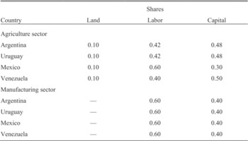
PRODUCTION FUNCTION PARAMETERS

Sources:
Based on Argentina: Garavaglia (1999), Sabato (1990), and Svec (1966); Uruguay: Barrán and Nahum(1967) and Barrios Pintos (1973); Mexico: Buve (1984), Bazant (1980), and Jarquín (1990); and Venezuela: Ardao (2002), Barral (1881), Brito Figueroa (2002), García Castro (1999), Pinero (1994), and Ríos de Hernández (1988).
The main exports varied by country. Argentina exported livestock by-products, wool, and wheat, while Uruguay's main exports were livestock by-products and wool. Mexico's main export goods were coffee, rubber, silver, and cotton. Finally, cacao and coffee represented the bulk of the exports from Venezuela. Based on this information, I estimated the shares of labor, capital, and land in the production function depending on the export good using balance sheets and accounting records of different productive units such as haciendas, plantations, and ranches as shown in Table 2.
To develop closed-form solutions, Cobb-Douglas production functions are adopted with an elasticity of substitution between land and labor of one. Using Cobb-Douglas production functions in equation 14 yields a friendly format to estimate the rent-wage ratio by feeding the model with terms of trade and ratios of factor endowments. Using the Cobb-Douglas standard format, equation 15 shows the reduced-form version used for estimation.

where α and θ are the shares of capital and β and γ are the shares of labor, and (1 – α− β) are the share of land.
Similar production shares are used for Argentina and Uruguay as both economies specialized in similar primary products. The capital requirements in the agricultural sector are consistent with the different types of agriculture. For the manufacturing sector, standard shares for capital and labor are assumed (Barro and Sala-i-Martin 2003). Capital is not fixed over time. During this period, capital investors sought to invest in areas with more labor internationally. As a result, the marginal productivity of capital equals the world price of capital.Footnote 26
INEQUALITY COUNTERFACTUALS
From the historical experience of Latin America, I explore several counterfactual scenarios.Footnote 27 The first two illustrate the importance of the numerous shocks that Latin America faced during the nineteenth century and their impact on inequality. By translating different initial conditions and shocks into time series, I use equation 15 to calculate the land rental to wage ratio. These calculations can be used to show the pressures that the actual historical shocks imposed on inequality over time. I consider three scenarios dealing with changes in land, labor, and terms of trade and their impact on inequality. The model predicts that a fixed land supply with a rising population would favor the landowning class by raising rents relative to wages and thus raising inequality. Expansions of land under cultivation holding the population constant would raise wages and lead to a lower rent-wage ratio and lower inequality. Finally, a rise in the terms of trade increases the return to land, which was often the more constrained factor of production, and thus raises the rent-wage ratio of inequality.
INITIAL CONDITIONS COUNTERFACTUALS
The persistence literature assigns a weighty role to initial conditions as determinants of the future inequality path. To judge the importance of these initial conditions, I trace the evolution of inequality of these four countries under two scenarios: in the first, each country starts the period with its actual historical endowments and then each experiences the same historical shocks and in the second each country has the same starting endowments and experiences the actual shocks that occurred in its history. Both exercises yield results that show small effects of initial conditions.
The first scenario considers country-specific initial conditions and each of the countries is subject to the same shocks over the course of the century. Consider country i with initial values for land (T 0), labor (L 0), and terms of trade  with corresponding inequality ineqi0 (calculated as the ratio between
 and
 ). Using the production sector parameters in Table 2, we assume now that country i is subject to the same shocks as the other countries with respect to change in terms of trade (change in ToT), land expansion (change in T), and immigration (change in L). These shocks (Xt) are calculated as the relative change of the decade-by-decade simple average of historical shocks in all the countries. Mathematically,

where  is the estimated shock at time
 are the country-specific initial conditions, and
 is the relative change of the average of
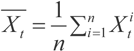 at time t = t for all countries with respect to
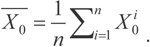 .
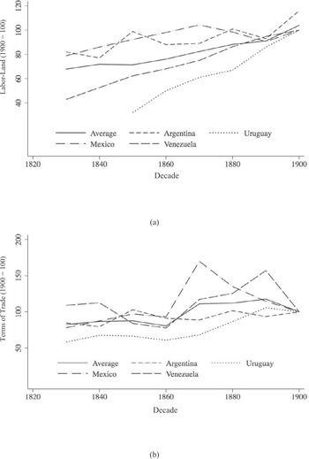
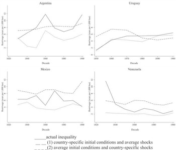
Figures 6A and 6B show the evolution of the labor-land ratio and the terms of trade for each country and the estimated average used in the first scenario. In Figure 6A, until about 1880 Argentina and Uruguay had higher labor-land ratios fueled by the large immigrant inflow while Mexico and Venezuela exhibited below average ratios. After 1880 nearly all the ratios converged to the mean. In Figure 6B, Uruguay experienced lower terms of trade than the average, Mexico and Venezuela had higher terms of trade than the average toward the end of the century, and Argentina hovered around the average throughout.
SCENARIO 1 - COUNTRY-SPECIFIC INITIAL CONDITIONS AND AVERAGE SHOCKS: (A) LABOR-LAND RATIOS: HISTORICAL VS. AVERAGE AND (B) TERMS OF TRADE: HISTORICAL VS. AVERAGE (1900 = 100)

HISTORICAL TRAJECTORIES AND COUNTERFACTUALS (1) COUNTRY-SPECIFIC INITIAL CONDITIONS AND AVERAGE SHOCKS AND (2) AVERAGE INITIAL CONDITIONS AND COUNTRY-SPECIFIC SHOCKS

Comparisons of the two simulation scenarios highlight the importance of the actual shocks to terms of trade and land-labor ratio relative to the importance of the initial starting conditions. The simulations based on common postcolonial shocks but country-specific initial conditions do not track the path of inequality over the century or match the ending point in the 1900s as well as simulations based on common starting conditions and country-specific shocks.
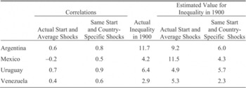
Figure 7 compares the simulated trajectory of inequality (the dashed lines) for the country-specific initial conditions and common shocks to its actual historical evolution (continuous lines). In the case of Argentina, the simulated inequality starts at a higher level than the actual inequality and then rises very slowly to around 9 by the end of the century.Footnote 28 It fails to capture the sharp rise in actual inequality to near 12 in the 1860s, the plunge to around 7 in the 1870s and the rise of to 12 again by 1900. Table 3 shows that the correlation between the actual rent-wage ratio and the simulated wage-rent ratio generated by the average shock is around 0.6, while the difference between the simulated ratio and the actual ratio in 1900 is −2.5 points.
CORRELATIONS BETWEEN ACTUAL RENT-WAGE RATIOS AND SIMULATED RENT-WAGE RATIOS FOR DIFFERENT ACTUAL STARTING CONDITIONS WITH SAME AVERAGE SHOCKS (1) VERSUS SAME AVERAGE START WITH COUNTRY- SPECIFIC SHOCKS (2) AND DIFFERENCES BETWEEN PREDICTED VALUES IN 1900 AND THE ACTUAL RENT-WAGE RATIOS

Notes:
Based on the model described above.
Sources:
See the Appendix.
Uruguay's simulated path presents a more volatile trajectory than the actual path that inequality followed. The simulation for Uruguay starts in the 1850s because evidence on the rent-wage is not available earlier. The simulated inequality is well above the actual value in the 1850s and 1860 but then falls to more than 20 percent below it in 1900. The correlation between the actual and simulated paths over the century in Table 3 is 0.7 and the difference between the ending points in 1900 is 1.5 points.
The simulated path for Venezuela deviated from the actual path more than in Argentina and Uruguay. Venezuela's simulated rent-wage ratio in Figure 7 fluctuates mildly between 6 and 5 over the century. In contrast, actual inequality in Venezuela started at a very high level in the 1830s and fell sharply to the 1840s before declining slowly over the rest of the century. The correlation between simulated and actual paths in Table 3 is 0.4 and the difference between the simulated and actual levels in 1900 is 2.4.
The largest differences between the simulated and actual path are in Mexico, where the correlation is −0.21 in Table 3. The simulated inequality path starts well above the actual path in the 1820s and stays above it throughout the century. By 1900 the simulated rent-wage ratio has risen to 11.5, as seen in Table 3. The actual path in Mexico fluctuated much more than the simulated path and declines to a low of 4.2 by early 1900s. As a result the correlation between the actual and simulated paths is −0.2 and there is a very large gap between the two paths of 7.3 points by the early 1900s.
The second set of simulations follows the opposite route. All countries start with the same initial conditions at the time of independence. These conditions are set at the average labor-land ratio of 68 and the terms of trade of 82. After evaluating equation 15 with these values, each country starts at a rent-wage ratio inequality measure of 2. Starting from these common initial conditions, the simulation assumes that each country experiences the actual shocks to the terms of trade and land-labor ratios over the course of the century. Argentina and Uruguay received a large inflow of immigrants from 1860 onwards. Mexico and Venezuela faced volatile terms of trade with a sizable drop towards the end of the century.
In this scenario, even though all countries start with the same initial conditions, once we let the actual changes in the labor-land ratio and terms of trade run their course, the simulated paths (dotted lines) tend to correspond more closely to the actual paths (continuous lines) in Figure 7 than they did in the first simulation. The correlations between actual and simulated rent-wage ratios in Table 3 document this. In each case, the correlation between the actual path and the simulated path based on common starting conditions with the actual shocks is more positive than the correlation between the actual path and the simulated path based on the country-specific start and the average-shocks.
The simulation with the common initial conditions and the actual shocks also come closer to predicting the actual rent-wage ratio in 1900 than the simulations based on the actual starts and common shocks. The gap between actual and predicted values in Uruguay was 0.7 and followed the actual path and was thus smaller than the 1.5 difference for the predictions for the country-specific starting conditions and common shocks. For Mexico, this difference amounted to −0.1 point and for Venezuela 0.6 point. Only in Argentina did the simulations based on the actual starting conditions and common shocks come closer to predicting the actual 1900 value than simulations based on the common-start and country-specific shocks.
On the other hand, the relative size of the prediction gaps for the two simulation methods varies from time period to time period. For example, comparisons in 1850 in Figure 7 show that the actual-start-common-shock simulated value is closer to the actual value than the common-start-actual-shock value in three of the four countries. Thus, the importance of differences in starting conditions in predicting future values varies over time.
The lessons learned from these counterfactuals are noteworthy. First, simulations that start at the same initial conditions for each country subject to actual shocks trace the fluctuations in the actual path followed by each country over the century more closely than ones that start at the country-specific starting conditions and experience the same shocks. Further, in three of the four cases, they come closer to predicting the rent-wage ratio at the end of the century. However, in other periods comparisons of the prediction gaps can change. The results suggest that differences in both starting values and shocks can teach us about what to expect for inequality in each time period. It is therefore important in examining long-range studies to look carefully not only at the endpoints of the periods but also the intervening activity.
COUNTERFACTUALS IN THE ABSENCE OF SHOCKS
To evaluate the importance of particular shocks on inequality, I build three counterfactuals. How would inequality have evolved in the absence of immigration, land expansion, or favorable terms of trade?
The first counterfactual exercise imposes a 50 percent decline in the terms of trade from the 1850 level. This shock is commensurate to the terms of trade decline that the region experienced during the Great Depression (Bulmer-Thomas 1994).Footnote 29 Theoretically, this will lead to a decline in the rent-wage ratio because the drop in export prices is expected to harm rents more than wages. For dramatic purposes, let us suppose that this shock took place between the 1850s and the 1860s and then the terms of trade stayed at 50 percent of the 1850 level for the rest of the century. My measure of the actual terms of trade index is 100 in 1900 for all countries. Given the actual values for the terms of trade in 1850, the 50 percent drop from 1850 to 1860 would have led to terms of trade in 1860 of 51, 34, 49, and 42 for Argentina, Uruguay, Mexico, and Venezuela respectively between 1850 and 1900. Then they would have remained at this level from 1860 to 1900.
EFFECT ON INEQUALITY OF A 50 PERCENT DECLINE IN TERMS OF TRADE FROM 1850 TO 1860 WITH NO CHANGE AFTER 1860

* All changes based on labor force and inequality 10-year averages.
** Endogenous labor supply only for Argentina and Uruguay.
Sources:
See the Appendix.
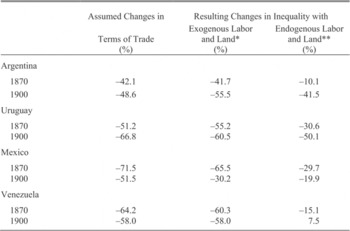
All four countries would have experienced a substantial decline in inequality had the terms of trade turned unfavorable in this way. By the turn of the twentieth century, the decline in inequality would have been around 30 percent in Mexico and nearly 60 percent in Uruguay and Venezuela. As shown in Table 4 for Argentina a 50 percent decline in the terms of trade in 1850 would have left the simulated terms of trade at 51, which is 42.1 percent below the actual terms of trade for Argentina in 1870 in column 1. If the amount of labor and land is not allowed to adjust to the difference, then the rent-wage ratio in 1870 would have ended up 41.7 percent lower than the actual experience in that year. If labor and land also were allowed to endogenously adjusted to the lower terms of trade, then the rent-wage ratio would have ended up only 10.1 percent below the actual ratio in 1870.
Had the terms of trade remained at 51 until 1900, the terms of trade would have been 48.6 percent lower than the historical value. If the labor and land supplies were left at their actual levels and were not allowed to change, the rent-wage ratio would have been 55.5 percent lower than the actual level in 1900. If land and labor were allowed to adjust endogenously, inequality would have been 41.5 percent lower.
Next, consider the impact of a shock to international migration on inequality. Even though most Latin American countries formulated policies to attract immigrants, very few succeeded.Footnote 30 In this case, only Argentina and Uruguay are considered as neither Mexico nor Venezuela received a sizable share of immigrants in the nineteenth century. The large inflows of migrants that arrived on the shores of the Southern Cone countries had a significant impact on the labor market.
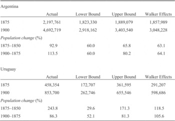
The “no-migration” counterfactual scenario calls for an estimation of the stock of population and labor force in the absence of these flows. By definition, total population growth is composed of two factors: natural growth and net immigration. Simply deducting the last item from population stock by year does not provide an accurate estimate, as it does not account for the indirect impact of immigration because immigrants will have children, who eventually will have children. Another complication arises from the possible crowding out of the native population by immigration—known as the “Walker effect.” To address this issue, I calculated three population stocks. The first estimation simply ignores the “Walker effect” and applies the overall population growth rate to premigration phase figures. The second estimation simply subtracts the stock of foreign born from total population. Following A. M. Taylor (1997), the third approach decomposes total population growth into natural growth and migration incorporating potential crowding out effect. The resulting estimations are presented in Table 5 for Argentina and Uruguay. I expect the first approach to lead to an upper-bound estimate of the impact of migration on population while the second one will lead to a lower-bound estimate. I favor the intermediate approach that attempts to capture the interaction between the native and the foreign population.
The next step involves calculating the labor force. The foreign and native populations had different rates of participation in the labor market. This difference is explained partly by age and gender composition. The “typical” migrant in the era of mass migration was an adult male. Fortunately, for the Argentine case, E. H. Kritz (1985) has explored this issue providing age, gender, and labor participation for the population by origin. His figures suggest that the labor force as a percentage of total population was 77 percent for foreigners and 44 percent for natives. These estimates are applied to the estimated populations to estimate the effective labor force for Argentina and Uruguay.
POPULATION ESTIMATIONS UNDER NO-IMMIGRATION COUNTERFACTUAL

Lower bound: Total population - Stock of foreign population.
Upper bound: Total population applying natural growth rate pre-immigration.
Walker effects: Based on regression p = a + bmt−1, where p is population growth, mt −1 is one-period lagged migration rate, a is the natural growth rate, and b is the estimated “Walker effect.”
Notes:
Under no-migration, we assume that b is equal to zero. Hence, we calculate population based on a.
The impact of migration on total population growth differed in Argentina and Uruguay. While the volume of migrants peaked in the 1880s, 34 percent of the population was foreign in 1862; however, the foreign share shrank to 23 percent by the turn of the century. In Argentina, this trend is reversed. Immigrants represented 11 percent of the population by 1869 and reached nearly 30 percent by 1900.
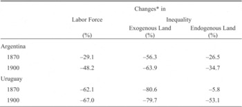
In the absence of migration, Argentina and Uruguay would have ended up with a much lower labor force. In Uruguay, by 1870 the no-migration labor force estimate would have been 62.1 percent lower than the actual figure (see column 1 of Table 6). Following this counterfactual, the model estimates a decrease in inequality of 80.6 percent by 1870 if the land frontier had followed the historical experience. If the amount of land were allowed to adjust endogenously to the changes in the labor force, the drop in inequality would have been dramatically lower at only 6 percent by 1870. The absence of migration would have had a larger effect by 1900. The no-migration labor force would have been 67 percent lower. With no change in the amount of land available, inequality would have been 80 percent lower. When the amount of land is allowed to adjust endogenously, the drop would only have been 53 percent. The difference between the inequality effect with endogenous land between 1870 and 1900 is due to the fact that by 1900 Uruguay's land use was much closer to the using up all land in the country than in 1870.
NO-MIGRATION EFFECT ON INEQUALITY

* All changes based on labor force and inequality 10-year averages.
Notes:
Based on the model described above.
Sources:
See the Appendix.
By the turn of the century, Argentina's no-migration labor force would have been 48.2 percent below its actual level. Under this counterfactual, inequality would have been 63.9 percent lower when land supply remains exogenous. In the case of endogenous adjustment of land, inequality would have declined only 34.7 percent.
The third counterfactual scenario evaluates the impact of keeping the supply of land fixed after 1850. This assumption implies only a modest increase in the land used in agricultural activities compared to the actual large expansion of historical experience. As a result, it accelerates the decline in the land-labor ratio, which then reduces the relative return to labor and thus raises the extent of inequality.
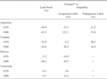
In this scenario, the stock of land in Argentina would have been 49.9 percent below its actual value in 1870 and 61.5 percent below in 1900 (Table 7, column 1). In that case, inequality would have increased by 53.5 percent by 1870 and more than 121 percent by 1900 if immigrant labor continued to flow to this country as it had historically. When the labor supply is allowed to adjust endogenously to the reduced stock of land, the increase in inequality would have been lower: 21.9 percent and 35 percent respectively. For Uruguay, the model predicts a smaller but still sizeable impact on inequality. By 1870 the land stock would have been 35 percent below the actual land stock, and the wage-rent ratio would have been 6.2 percent higher with the actual change in labor supplied, but 20.2 percent higher if the labor supply adjusted to the different conditions. By 1900 Uruguay's land stock would have been 42.8 percent lower than the actual stock, and the wage-rent ratio would have escalated by 49.3 percent had the actual labor supply been in place, but only 16.9 percent if workers had responded to the lower availability of land by not migrating there.
EFFECT OF NO-FRONTIER EXPANSION ON INEQUALITY

* All changes based on land stock and inequality 10-year averages.
Notes:
Based on the model described above.
Sources:
See the Appendix.
The actual stock of land did not grow much in Venezuela after 1850, which is why the absence of frontier expansion in the simulation only cut land stock in Table 3 by 4.3 percent in 1870 and by 9.7 percent in 1900. As a result, the impact on rent-wage ratios with exogenous changes in labor supply were similarly small at 5.6 percent by 1870 and 12.2 percent by 1900. In Mexico, the frontier expanded mostly after 1870. Without that expansion the land available would have been 40.1 percent lower in Mexico by 1900, and inequality would have been 54.7 percent higher with the actual amount of labor that was there.Footnote 31
CONCLUDING REMARKS
Latin America today exhibits “excess inequality,” a higher level of inequality given its economic development than is found in many countries. Many claim that the long arm of colonial history explains this characteristic. I concentrate on the postcolonial period from the 1820s to the 1900s to explore the question of inequality persistence. Using secondary sources and freshly unearthed data from Latin American archival sources, this article presents new estimates of Latin American inequality during the nineteenth century. An equilibrium equation from a theoretical model shows the anticipated relationship between inequality, the terms of trade, and land-labor ratios.
Inequality in Latin America varied substantially throughout the nineteenth century. Moreover, the trajectory was not uniform in all countries. The external market conditions paired with the particular evolution of factor endowments throughout the century were decisively linked to the trajectory of inequality. Factor endowments mattered and migration flows and annexation of additional land led to sizable fluctuations in the relative scarcity of factors of production and their returns. Mass migration to Uruguay and Argentina led to lower land-labor ratios and thus increases in the rent-wage ratio measure of inequality. Yet, as land was annexed the impact of migration was dampened. As the countries increased their participation in world trade, the income distribution increasingly responded to changes in the country’ terms of trade.
The results indicate that inequality in Uruguay and Argentina rose during the era of globalization, while it decreased in Mexico and Venezuela. The rise in inequality in Argentina and Uruguay is explained by the impact of favorable terms of trade and international migration; however, the effect was dampened by significant land annexation. On the other hand, the decline in Mexican and Venezuelan inequality is related to decreasing terms of trade amplified by the expansion of available arable land.
The theoretical model used here allows us to trace the magnitude of the impact of changing terms of trade and factor endowments on inequality. Furthermore, this model also highlights the importance of historical shocks in the evolution of inequality. The simulation exercises show that changes in the stock of land, labor, and in the terms of trade play an important role in determining inequality. Overall, this article shows the importance of shocks in shaping the evolution of inequality over time. This suggests that the role of colonial initial conditions has been overemphasized in the literature.
This article was partly developed while in residence at the World Institute for Development Economics Research, United Nations University. I thank the participants at the GlobalEuronet Research Networking Summer School, the WIDER-UNU seminar, the UC Davis economic history seminar, the UC Berkeley economic history seminar, the Stanford economic history seminar, and the Latin American Economic History conference. I am indebted to my advisors Peter H. Lindert and Alan M. Taylor, Luis Bértola, Amílcar Challú, Aurora Gómez Galvarriato, Price Fishback, Carlos Newland, Jeffrey Williamson, and two anonymous referees. All errors remain mine. I acknowledge research funding provided by the American Economic History Association, the All-UC Economic History Group, the UC Davis Agriculture History Center, the UC Davis Center for the Evolution of the Global Economy, the UC Davis Institute of Governmental Affairs, and the Centro de Estudios y Programas Interamericanos.
Appendix: Data Sources
The long-term series presented and used in this article are the result of original archival data collection and secondary sources when available. Especially for earlier periods, the data are from archives in Latin America, Spain, and the United Kingdom. Wage Rates: Nominal wages correspond to urban workers in major metropolitan areas for unskilled work. Typical occupations include peons, servants, and doormen. At times, payment consisted of a monetary and an in-kind components. When noted, the in-kind part was added to calculate the full remuneration. Wages correspond to annual payments and were recorded annually when possible.
Argentina: For the early data, 1810–1860, salaries are from the Women's and Men's Hospitals in Buenos Aires.Footnote 32 The series was complemented with data from F. E. Barba (1999) and spliced for the period 1885–1914 with data from R. Cortés Conde (1979).
Mexico: For 1820–1900 wages are from Mexico City's payroll records at different public institutions such as the central wholesale marketplace, hospices, prisons, convents, hospitals, and schools.Footnote 33
Uruguay: The series spanning from 1805 through 1889 is from the Charity Hospital in Montevideo.Footnote 34 For the rest of the period, 1890–1914, the series was spliced with data from Bértola and Williamson (2006).
Venezuela: Wage data was available for Caracas in annual national budgets.Footnote 35
Land Rental: Land prices were converted to land rental values using the D. Jorgenson (1967) derivation. In a nutshell, the land rental value is the product of value and the combination of the prevailing interest rate and the depreciation rate for land. Given the increasing integration of the Latin American countries to the world capital markets, it is important to take into account the converging interest rate. For further discussion on capital market integration and land rentals, see M. Obstfeld and Taylor (2005) and Williamson (2007). The interest rate was obtained from the Global Financial Database. For earlier years (1820–1830), quotes from the British newspapers Common Sense, Course of the Exchange, and The Colonist were collected from the British Library newspaper collection in Colindale.
Argentina: Land prices were compiled from recorded private sales in the Buenos Aires province. For the later period (1894–1913), this series was spliced with data from Cortés Conde (1979).Footnote 36
Mexico: Land prices from D. Brading (1978) and J. Gomez Serrano (2000) complemented with a few observations from the National Archives.Footnote 37 The regions included are El Bajio and Aguascalientes.
Uruguay: Data correspond to 5-year price averages as presented by Bárran and Nahum (1967). The regions cover the entire geographical area, i.e., South, Litoral, North, and Center.
Venezuela: CDCH (1971) provides sales of private lands over the entire period. The geographical scope covers the states of Apure, Barcelona, Barinas, Barquisimeto, Carabobo, Caracas, Cedeño, Coro, Cumacatar, Cumaná, Guárico, Maracaibo, Maturin, Merida, Miranda, Portuguesa, Táchira, and Yaracuy.
Terms of Trade: When available, published terms of trade were used. In most cases, for the earlier decades, no data existed. The standard methodology was to obtain export and import prices for the main commodities and compose a index with weights given by the overall composition of trade. In general, both exports and imports were concentrated in a handful of commodities. To minimize the bias from different commodity baskets, a Fisher index was calculated.
Argentina: The calculation of terms of trade followed Newland (1998)'s methodology. Export and import prices from this source are available until 1870. For 1870 to 1885 the same sources were used by the author. The weights assigned to the main export and import products are based on historical export and import volumes from Dirección General de Estadística (1916). From 1885 onwards both series were spliced with data from O. Ferreres (2005).
Mexico: Terms of trade are taken from L. K. Salvucci and R. J. Salvucci (2000).
Uruguay: It is not until 1880s that published terms of trade are available from Bértola (2000). Following a similar methodology as in the case of Argentina, the rest of the series was calculated using commodity prices from Uruguayan newspapers such as Britannia, Comercio del Plata, and El Nacional housed at the Uruguayan Public Library. Dirección de Estadística General de la República (1878) and Consejo Nacional de Administración.
Uruguay: Consejo Nacional de Administración Uruguay (1925) provided useful data for the weights chosen.
Venezuela: A. Baptista (2006) provides an annual terms of trade series.
Land Stock: In all cases, I estimated the expansion of the expansion of land based on public records of public land sales. In some cases, these lands were previously leased and as such we only added the acreage when in use not when sold.
Argentina: M. E. Infesta (2003) and M. Valencia (2005) provide detail records of land sales for the Buenos Aires province. We complemented these data with figures in the Comisióßn Directiva del Censo (1898) and Comisión Directiva del Censo (1919).
Mexico: R. Qamber (1992) supplies the number of acres sold to the public until 1910s. To this stock we added the land given free to the poor. I cross-checked this information with benchmark figures for the 1866–1894 period by A. Peñafiel (1894).
Uruguay: Barrán and Nahum (1967) offers data on public and private land sales for selected decades starting in 1830 through 1930s.
Venezuela: Estimates taken from O. Delahaye (2003).
Population: Population and labor figures were obtained mostly from censuses. Unskilled labor was computed by taking into account illiterate population over 14 years of age.
Argentina: Before mid-nineteenth century, from E. Maeder (1969) and followed by A. E. Lattes (1968).
Mexico: From E. Malvido and M. A. Cuenya (1993) and Malvido (2006).
Uruguay: Earlier data from G. Mortara (1947) supplemented with E. Narancio and F. C. Calamet (1939). Immigration figures from J. C. Petrucelli and J. C. Fortuna (1976) and A. Pacheco (1892).
Venezuela: From M. Izard (1970) and Junta Directiva del Censo (1891).