Introduction
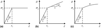
In recent studies, interest has been intensified in the development of indentation-based methods extracting the elastic–plastic properties. A number of theoretical and semi-theoretical methods have been developed.[ Reference Choppacoop, Dao and Suresh 1 – Reference Yu, Feng, Yang, Peng, Lu and Zhang 10 ] In most of these studies, the linear elastic power-law hardening constitutive model was generally adopted. In fact, however, the stress–strain behaviors of many metals are better described by the linear elastic and perfectly plastic constitutive model or the linear elastic linear hardening constitutive model (see Fig. 1).
Three typical stress–strain relationships. (a) Linear elastic and perfectly plastic, (b) linear elastic and linear hardening, and (c) linear elastic and power-law hardening.[ Reference Yu, Yang, Feng, Huan, Peng and Zhang 11 ] (© Materials Research Society, 2015, Reprinted with permission.)

A general stress–strain relationship for the material can be written as
 $$\tilde \sigma = \left\{ \matrix{E\tilde \varepsilon {\rm} \hskip 6pt(\tilde \varepsilon \lt \varepsilon _{\rm y} ), \hfill \cr f\,(\tilde \varepsilon ){\rm} (\tilde \varepsilon \ge \varepsilon _{\rm y} ), \hfill} \right.$$
where
 $\tilde \sigma $
and
 $\tilde \varepsilon $
are the equivalent stress and strain, respectively; E is the elastic modulus; ε
y is the yield strain; the function
 $f\,(\tilde \varepsilon )$
is the constitutive equation of material, which for perfectly plastic materials takes the form,
 $$\tilde \sigma = E\varepsilon _{\rm y}, $$
while for linear hardening materials, it can be written as
 $$\tilde \sigma = E_{\rm p} \tilde \varepsilon + (E - E_{\rm p} )\varepsilon _{\rm y}, $$
and for power-law hardening materials, it can be written as
 $$\tilde \sigma = E\varepsilon _{\rm y}^{1 - n} \tilde \varepsilon ^n, $$
where E p is the hardening modulus for linear hardening materials, and n is the hardening exponent for power-law hardening materials. These three forms of stress–strain relationship are shown in Fig. 1. It should be pointed out that perfectly plastic materials is included in linear hardening materials as a special case (E p = 0), and it is also included in power-law hardening materials as a special case (n = 0). But it is usually considered as a classical constitutive form. So they are discussed as three separate forms in this paper.
It has been shown that the parameters of the typical constitutive models of metals can be determined by instrumented spherical indentation tests.[ Reference Yu, Yang, Feng, Huan, Peng and Zhang 11 ] But the elastic–plastic constitutive models of the metals must be known in advance in order to choose the appropriate method. For a material with unknown elastic–plastic constitutive model, it is difficult to decide which method should be chosen. It has been shown that the stress–strain relationships may not be uniquely determined from indentation loading and unloading curves obtained using a conical or pyramidal indenter.[ Reference Cheng and Cheng 12 ] In this paper, we will discuss the feasibility of distinguishing the elastic–plastic constitutive models by spherical indentation.
Methods to determine elastic–plastic parameters for three typical elastic–plastic constitutive models
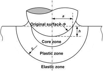
In our previous work, methods to determine elastic–plastic parameters for three typical constitutive models by instrumented spherical indentation had been developed.[ Reference Buljak, Cocchetti, Cornaggia and Maier 9 – Reference Yu, Yang, Feng, Huan, Peng and Zhang 11 ] Based on the spherically symmetric assumption in the expanding cavity model (ECM)[ Reference Johnson 13 ] (see Fig. 2) and the Lamé’s elastic solution, the equations of total loading work (W t) and unloading work (W u) were derived.[ Reference Yu, Yang, Feng, Huan, Peng and Zhang 11 ]
Expanding cavity model in which the deformation area below the indenter is divided into three parts. The effect of pile-up or sink-in is equivalent to some fraction of hydrostatic core volume displaced by indenter.[ Reference Yu, Yang, Feng, Huan, Peng and Zhang 11 ] (© Materials Research Society, 2015, Reprinted with permission.)

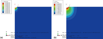
There are two basic hypotheses for ECM: (1) the displacement field produced by the indenter is approximately spherically symmetric; (2) the material under the indenter can be divided into three parts, namely, a core zone (r < a), a plastic zone (a < r < c), and an elastic zone (r > c), where a is the radius of the core zone and c is the radius of the boundary of the plastic and elastic zones. They can be confirmed by the result of a popular finite-element method (FEM) modeling (see Fig. 3).
The result of a popular FEM modeling, which can confirm the two basic hypothesis of ECM: (a) the displacement distribution confirms that the displacement field produced by the indenter is approximately spherically symmetric; (b) the mises stress distribution confirms the partition under the indenter.

In this model, seven parameters (radial displacement u r ; strain ε r , ε θ , and ε φ ; stress σ r , σ θ , and σ φ ) are taken into consideration. Relationships about these parameters include the geometric equations as
 $$\left\{ \matrix{\varepsilon _r = \displaystyle{{{\rm d}u_r} \over {{\rm d}r}}, \hfill \cr \varepsilon _\theta = \varepsilon _\varphi = \displaystyle{{u_r} \over r}, \hfill} \right.$$
and the balance equation as
 $$\displaystyle{{{\rm d}\sigma _r} \over {{\rm d}r}} + 2\displaystyle{{\sigma _r - \sigma _\theta} \over r} = 0.$$
The equivalent stress and strain[ Reference Hill 14 ] are
 $$\eqalign{\tilde \sigma & = \displaystyle{1 \over {\sqrt 2}} \sqrt {(\sigma _r - \sigma _\theta )^2 + (\sigma _\theta - \sigma _\varphi )^2 + (\sigma _\varphi - \sigma _r )^2} \cr & = \sigma _\theta - \sigma _r,}$$
 $$\eqalign{\tilde \varepsilon & = \displaystyle{{\sqrt 2} \over 3}\sqrt {(\varepsilon _r - \varepsilon _\theta )^2 + (\varepsilon _\theta - \varepsilon _\varphi )^2 + (\varepsilon _\varphi - \varepsilon _r )^2} \cr & = \displaystyle{2 \over 3}(\varepsilon _\theta - \varepsilon _r ).}$$
Assuming materials are incompressible (viz. the Poisson ratio ν = 0.5)[ Reference Gao and Jing 5 ], argued that radial displacement, u r , is related to the volume of the materials excluded by the indenter, V. The relationship can be written as
 $$V = \displaystyle{2 \over 3}\pi \left[ {(r + u_r )^3 - r^3} \right] = \displaystyle{2 \over 3}\pi u_r (3r^2 + 3ru_r + u_r^2 ).$$
It is easy to obtain
 $u_r /r = \root 3 \of {3V/(2\pi r^3 ) + 1} - 1$
. By considering the ratio of depth (h/R) as a constant 0.3,[
Reference Jiang, Zhang, Feng, Yang and Liang
7
]
u
r
/r is not larger than 0.1 and decreases rapidly. It means that a small deformation assumption (u
r
≪ r) is reasonable and Eq. (9) can be simplified into
 $$V = 2\pi u_r r^2, $$
and u r can be written as
 $$u_r = \displaystyle{V \over {2\pi r^2}}. $$
Substituting Eq. (11) into Eq. (5) yields
 $$\left\{ \matrix{\varepsilon _r = - \displaystyle{V \over {\pi r^3}}, \hfill \cr \varepsilon _\theta = \varepsilon _\varphi = \displaystyle{V \over {2\pi r^3}}. \hfill} \right.$$
By substituting Eq. (12) into Eq. (8), the equivalent strain can be written as
 $$\tilde \varepsilon = \displaystyle{V \over {\pi r^3}}. $$
At the outer boundary of the plastic zone
 $$\left. {\tilde \varepsilon} \right \vert _{r = c} = \displaystyle{V \over {\pi c^3}} = \varepsilon _{\rm y}. $$
By substituting Eq. (14) into Eq. (13), the relationship between equivalent strain and radius is
 $$\tilde \varepsilon = \displaystyle{{c^3} \over {r^3}} \varepsilon _{\rm y}. $$
The energy density can be written as
 $$w = \int {\tilde \sigma {\rm d}\tilde \varepsilon}. $$
The equations of total loading work (W t) and the unloading work (W u) can be obtained by integrating of Eq. (16).[ Reference Yu, Yang, Feng, Huan, Peng and Zhang 11 ]
The similarity solution, Meyer's index (m), was used to solve the elastic–plastic parameters by combining with the equations of total loading and unloading works.[ Reference Jiang, Zhang, Feng, Yang and Liang 7 ] Finite-element analysis (FEA) was carried out using ABAQUS to correct the equations.[ Reference Jiang, Zhang, Feng, Yang and Liang 7 ] The corrected equations for calculating the total loading work (W t) and unloading work (W u) for different constitutive models can be written as follows.
For linear elastic perfectly plastic constitutive model,
 $$\left\{ \matrix{W_{\rm t} = \kappa _1 \pi E\varepsilon _{\rm y} ^2 \left[ {\displaystyle{1 \over 3}a^3 + c^3 \left( {2\ln \displaystyle{c \over a} - \displaystyle{{c^3} \over {a^3}} \varepsilon _{\rm y} + \displaystyle{2 \over 3}} \right)} \right], \hfill \cr W_{\rm u} = 3\kappa _2 \pi E\varepsilon _{\rm y} ^2 a^3 \left( {\displaystyle{1 \over 3} - \ln \displaystyle{a \over c}} \right)^2, \hfill} \right.$$
where E is the elastic modulus, a is the radius of the hemispherical hydrostatic core, c is the radius of the hemispherical plastic zone (see Fig. 2) and κ 1, κ 2 are the correction factors and given as
 $$\left\{ \matrix{\kappa _1 = - 0.09822\log ^2 (\varepsilon _{\rm y} ) - 0.2251\log (\varepsilon _{\rm y} ) + 1.136, \hfill \cr \kappa _2 = 0.1977\log ^2 (\varepsilon _{\rm y} ) + 1.624\log (\varepsilon _{\rm y} ) + 3.694. \hfill} \right.$$
For linear elastic linear hardening constitutive model,
 $$\left\{ \eqalign{W_{\rm t} & = \lambda _1 \pi E\varepsilon _y ^2 \cr & \quad \times \left\{ {\displaystyle{1 \over 3}\displaystyle{{E_{\rm p}} \over E}\displaystyle{{c^6} \over {a^3}} + \displaystyle{1 \over 3}\left( {1 - \displaystyle{{E_{\rm p}} \over E}} \right)a^3 + 2\left( {1 - \displaystyle{{E_{\rm p}} \over E}} \right)c^3 \ln \displaystyle{c \over a}} \right. \cr & \quad\left. { + \, c^3 \left[ {\displaystyle{{E_{\rm p}} \over E}\displaystyle{{c^3} \over {a^3}} + \left( {1 - \displaystyle{{E_{\rm p}} \over E}} \right)} \right]\left( {\displaystyle{2 \over 3} - \displaystyle{{c^3} \over {a^3}} \varepsilon _{\rm y}} \right)} \right\}, \cr W_{\rm u} & = {\rm 3}\lambda _2 \pi E\varepsilon _y ^2 a^3 \left[ {\displaystyle{1 \over 3}\displaystyle{{E_{\rm p}} \over E}\displaystyle{{c^3} \over {a^3}} + \left( {1 - \displaystyle{{E_{\rm p}} \over E}} \right)\left( {\displaystyle{1 \over 3} - \ln \displaystyle{a \over c}} \right)} \right]^2, \cr m & = \left[ { - 7.807 \times 10^6 \left( {\displaystyle{{E_{\rm p}} \over E}} \right)^3 + 1.217 \times 10^6 \left( {\displaystyle{{E_{\rm p}} \over E}} \right)^2} \right. \cr & \quad \left. { - 8.186 \times 10^4 \left( {\displaystyle{{E_{\rm p}} \over E}} \right) + 7232} \right]\varepsilon _y ^2 \cr & \quad + \left[ \!\!{ - 5003\left( {\displaystyle{{E_{\rm p}} \over E}} \right)^3 + 5136\left( {\displaystyle{{E_{\rm p}} \over E}} \right)^2 - 277.8\left( {\displaystyle{{E_{\rm p}} \over E}} \right) - 83.91} \!\!\right]\varepsilon _{\rm y} \cr & \quad + \left[\! {1330\left( {\displaystyle{{E_{\rm p}} \over E}} \right)^3 - 302.6\left( {\displaystyle{{E_{\rm p}} \over E}} \right)^2 + 24.87\left( {\displaystyle{{E_{\rm p}} \over E}} \right) + 2.457} \!\right],} \right.$$
where E p is the hardening modulus and λ 1, λ 2 are the correction factors and given as
 $$\left\{ \eqalign{\lambda _1 & = \left[ { - 321.9\left( {\displaystyle{{E_{\rm p}} \over E}} \right)^3 + 97.29\left( {\displaystyle{{E_{\rm p}} \over E}} \right)^2} \right. \cr & \qquad \left. { - 8.627\left( {\displaystyle{{E_{\rm p}} \over E}} \right) + 0.07456} \right]\log ^2 (\varepsilon _{\rm y} ) \cr & \qquad + \left[ { - 2037\left( {\displaystyle{{E_{\rm p}} \over E}} \right)^3 + 559.1\left( {\displaystyle{{E_{\rm p}} \over E}} \right)^2} \right. \cr & \qquad \left. { - \,45.16\left( {\displaystyle{{E_{\rm p}} \over E}} \right) + 0.3521} \right]\log (\varepsilon _{\rm y} ) \cr & \qquad + \left[ { - 2681\left( {\displaystyle{{E_{\rm p}} \over E}} \right)^3 + 704.2\left( {\displaystyle{{E_{\rm p}} \over E}} \right)^2} \right] \cr & \qquad \left. { - 54.80\left( {\displaystyle{{E_{\rm p}} \over E}} \right) + 1.616} \right], \cr \lambda _2 & = \left[ {942.8\left( {\displaystyle{{E_{\rm p}} \over E}} \right)^3 - 20.94\left( {\displaystyle{{E_{\rm p}} \over E}} \right)^2} \right. \cr & \qquad \left. { - 20.54\left( {\displaystyle{{E_{\rm p}} \over E}} \right) + 0.8147} \right]\log ^2 (\varepsilon _{\rm y} ) \cr & \qquad + \left[ {1189\left( {\displaystyle{{E_{\rm p}} \over E}} \right)^3 + 634.1\left( {\displaystyle{{E_{\rm p}} \over E}} \right)^2} \right. \cr & \qquad \left. { - 146.0\left( {\displaystyle{{E_{\rm p}} \over E}} \right) + 3.939} \right]\log (\varepsilon _{\rm y} ) \cr & \qquad + \left[ { - 784.2\left( {\displaystyle{{E_{\rm p}} \over E}} \right)^3 + 1187\left( {\displaystyle{{E_{\rm p}} \over E}} \right)^2} \right. \cr & \qquad \left. { - 191.0\left( {\displaystyle{{E_{\rm p}} \over E}} \right) + 5.918} \right].} \right.$$
For linear elastic power-law hardening constitutive model,
 $$\left\{ \eqalign{W_{\rm t} &= \eta _1 \pi E\varepsilon _y ^2 \left[ {\displaystyle{{2n} \over {3(n + 1)}}c^3 - \displaystyle{{n - 1} \over {3(n + 1)}}a^3} \right. \cr & \qquad + \displaystyle{{2c^3} \over {3n(n + 1)}}\left( {\displaystyle{{c^{3n}} \over {a^{3n}}} - 1} \right) + \displaystyle{{c^{3(n{\rm +} 1)}} \over {a^{3n}}} \left( {\displaystyle{2 \over 3} - \displaystyle{{c^3} \over {a^3}} \varepsilon _{\rm y}} \right), \cr W_{\rm u} & \quad = \displaystyle{{\eta _2} \over {3n^2}} \pi E\varepsilon _y ^2 a^3 \left( {\displaystyle{{c^{3n}} \over {a^{3n}}} + n - 1} \right)^2, \cr m & = (8306n^2 - 2762n - 1805)\varepsilon _{\rm y}^2\cr & \qquad + ( - 6.296n^2 - 81.22n + 71.78)\varepsilon _{\rm y} \cr & \qquad + ( - 1.222n^2 + 2.724n + 1.723),} \right.$$
where n is the hardening exponent and η 1, η 2 are the correction factors and given as
 $$\left\{ \eqalign{\eta _1& = (0.2984n^2 - 0.01787n - 0.1293)\log ^2 (\varepsilon _{\rm y} ) \cr &\qquad + (3.072n^2 - 1.708n - 0.3819)\log (\varepsilon _{\rm y} ) \cr &\qquad + (4.048n^2 - 3.092n + 0.9490), \cr \eta _2& = (1.804n^2 - 1.364n + 0.1134)\log ^2 (\varepsilon _{\rm y} )\cr &\qquad {\rm +} \, (9.849n^2 - 9.176n + 1.271) \log(\varepsilon _{\rm y} ) \cr &\qquad {\rm +} \,(10.78n^2 - 10.541n + 3.316).} \right.$$
Finite-element method
FEM was used to determine the accuracy of the analytical expressions. Plastic parameters used in the FEM calculations cover most of metal materials. Elastic modulus (E) is 210 GPa, which is approximately equal to the elastic modulus of steel. To make these simulations consistent with reality, the elastic modulus takes value of 210 GPa, Poisson's ratio takes value of 0.3, the yield strain ranges from 0.001 to 0.01, the hardening slope E p/E ranges from 0.02 to 0.10 (for linear hardening) and hardening exponent n ranges from 0.1 to 0.5 (for power-law hardening), which covers most engineering metals. Interface friction is neglected to match the assumption in theoretical analysis.
Method to identify the elastic–plastic constitutive models
The total loading and unloading works are chosen as analytical parameters in the method to determine the elastic–plastic parameters. It is easily known that the total loading and unloading works are determined by the stress distribution at the end of the loading. Due to the complexity of the stress distribution under the indenter, different constitutive models (i.e. elastic–plastic constitutive models) with particular material parameters may lead to the same stress distribution. By analyzing the deformation process for the three typical constitutive models qualitatively, we found out that the deformation path to reach the same stress distribution varies for different constitutive models. Therefore, the analytical parameters chosen by the method to distinguish the constitutive models should be able to describe the deformation process of the material. Because the linear elastic perfectly plastic constitutive model can be considered as a special case of the other two constitutive models, it will not be discussed separately in the present work.
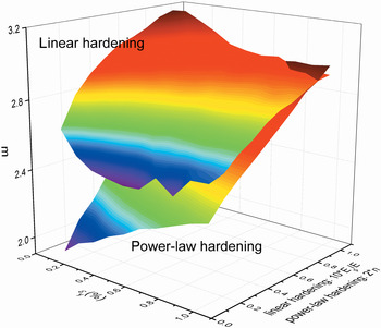
The Meyer's index (m) is the slope of the logarithmic loading curve, which is related to the loading process and is able to describe the deformation path of the material. The Meyer's indices for linear elastic linear hardening and linear elastic power-law hardening constitutive models with various plastic parameters calculated from the finite element results were illustrated in Fig. 4. Because of the different ranges of the hardening parameters (0.01 ≤ E p/E ≤ 0.1 for linear hardening and 0.05 ≤ n ≤ 0.5 for power-law hardening), the normalization of the hardening parameters (10E p/E and 2n) are adopted and used as the coordinate point. The result shows that the Meyer's indices of the two constitutive models with the similar plastic parameters are distinct, and the difference increases with the decrease of the plastic parameters ε y, 10E p/E and 2n.
The relationship between Meyer's indices and plastic parameters with the different constitutive models of linear hardening and power-law hardening.

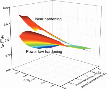
Considering the loading process, the differences of deformation path resulted in different energy accumulation rates in the different stages of loading. The ratio of loading work at half-max depth (W half) and total loading work (W t), which will be referred as “half depth energy accumulation rate” (W half/W t), is analyzed. The correlations between half depth energy accumulation rates and plastic parameters are shown in Fig. 5. It is clear that the half depth energy accumulation rates for linear hardening and power-law hardening deviate from each other, and the discrepancy increases as the yield strain and the hardening parameters decreasing.
The relationship between half depth energy accumulation rates and plastic parameters with the different constitutive models of linear hardening and power-law hardening.

From above analysis, m and W half/W t can be correlated with the deformation path, and the relationships between m and W half/W t are different for different constitutive models. They can be used as the analytical parameters in the method to distinguish the stress–strain relationships.
m and W half/W t can be expressed as a function of plastic parameters, respectively.
 $$\left\{ \matrix{m = f\,(\varepsilon _{\rm y}, E_{\rm p} /E),\quad {\rm for}\;{\rm linear}\;{\rm hardening,} \hfill \cr m = f\,(\varepsilon _{\rm y}, n),\quad {\rm for}\;{\rm power - law}\;{\rm hardening,} \hfill} \right.$$
 $$\left\{ \matrix{W_{{\rm half}} /W_{\rm t} = f(\varepsilon _{\rm y}, E_{\rm p} /E)\;{\rm for}\;{\rm linear}\;{\rm hardening,} \hfill \cr W_{{\rm half}} /W_{\rm t} = f(\varepsilon _{\rm y}, n)\;{\rm for}\;{\rm power - law}\;{\rm hardening}{\rm.} \hfill} \right.$$
Therefore, it can be deduced that there is a functional relationship between m and W half/W t
 $$W_{{\rm half}}/W_{\rm t} = f\,(m). $$
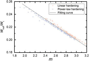
The distribution of half depth energy accumulation rates with Meyer's indices is shown in Fig. 6, which was obtained by the FEA. It is evident that the half depth energy accumulation rate decreases linearly with the increase of Meyer's index. The distribution points for linear hardening and power-law hardening can be clearly separated from each other by a dividing line as shown in Fig. 6.
The relationship between half depth energy accumulation rates and Meyer's indices with the different constitutive models of linear hardening and power-law hardening.

Fitting the dividing line using the least-squares method leads to
 $$W_{{\rm half}} /W_{\rm t} = - 0.0538m + 0.3612.$$
The result can be drawn from Fig. 6. If W half/Wt > − 0.0538m + 0.3612, then the strain hardening model is linear hardening. If W half/Wt < − 0.0538m + 0.3612, then the strain hardening model is power-law hardening. Equation (25) can then be used for identification of the elastic–plastic constitutive model by instrumented spherical indentation. W half/W t, m in Eq. (25) can be obtained directly from the load–depth curves.
To facilitate subsequent discussion, Eq. (25) will be rewritten as Eq. (26), and denoted as a letter D. It can be called as “the identification factor”. It is evident from Fig. 6 that the strain hardening model is linear hardening for D > 0, and the strain hardening model is power-law hardening for D < 0. This can be used as an identification criterion for distinguishing the strain hardening model.
 $$D = W_{{\rm half}} /W_{\rm t} + 0.0538m - 0.3612.$$
Experiments and discussion
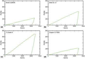
Instrumented spherical indentation tests were performed on four materials, i.e. Brass C28000, Steel Gr. D, Ti Grade 5, and Copper C11000, using a Nano Indenter XP (MTS) to validate our method. The typical indentation load–depth curves for Brass C28000, Steel Gr. D, Ti Grade 5, and Copper C11000 were shown in Fig. 7. The analytical parameters W half/W t, m obtained from the loading curve were listed in Table 1.
The typical load–depth (F–h) curves of the four materials tested by instrumented spherical indentation. (a) Brass C28000, (b) Steel Gr. D, (c) Ti Grade 5, (d) Copper C11000.

Analytical parameters of the four materials obtained by instrumented spherical indentation tests.

Substituting the analytical parameters W half/W t, m into Eq. (26), we get the identification factors D C28000 = 0.016 > 0 for Brass C28000, D Gr. D = −0.0026 < 0 for Steel Gr. D, D Ti.G5 = −0.018 < 0 for Ti Grade 5, and D C11000 = 0.0012 > 0 for Copper C11000. According to identification criterion, we can forecast that the strain hardening models of Brass C28000 and Copper C11000 are linear hardening, and those of Steel Gr. D and Ti Grade 5 are power-law hardening.
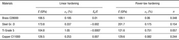
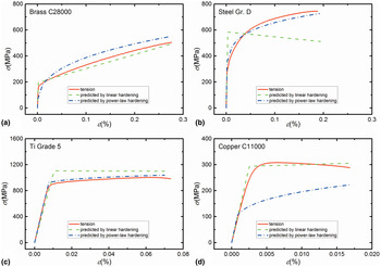
The elastic–plastic parameters of Brass C28000, Steel Gr. D, Ti Grade 5, and Copper C11000 were determined using both methods for linear hardening (Eqs. 3 and 4) and power-law hardening (Eqs. 5 and 6). Table 2 lists two groups of elastic–plastic parameters for each material determined by two methods.
Material parameters determined by the two methods of linear hardening and power-law hardening.

Each group of material parameters are substituted into the corresponding elastic–plastic constitutive models to predict the stress–strain curves. The curves are compared with the conventional uniaxial tensile results,[ Reference Jiang, Zhang, Feng, Yang and Liang 7 ] as shown in Fig. 8. The result shows that for Brass C28000 and Copper C11000, it matches better using the method for linear hardening; and for Steel Gr. D and Ti Grade 5, it matches better using the method for power-law hardening. It thus demonstrates that D > 0 can be used as the criterion to identify the linear elastic linear hardening constitutive model and D < 0 can be considered as the criterion for identification of the linear elastic power-law hardening constitutive model.
The typical stress–strain curves predicted by different constitutive models and compared with the conventional uniaxial tensile tests. (a) Brass C28000, (b) Steel Gr. D, (c) Ti Grade 5, (d) Copper C11000.

Conclusion
A method to distinguish the elastic–plastic constitutive models is developed based on instrumented spherical indentation technique. Through qualitative analysis, half depth energy accumulation rate and Meyer's index are chosen as the analytical parameters. FEA shows that an approximate linear relationship exists between the half depth energy accumulation rate and Meyer's index. There is a clear dividing line between the data points for different constitutive models (see Fig. 6). Fitting the dividing line to develop the method for distinguishing the elastic–plastic constitutive models, and put forward the concept of the identification factor. The experimental results of Brass C28000, Steel Gr. D, Ti Grade 5, and Copper C11000 confirm the validity of the newly proposed method. The significance of this paper is combining the forward analysis and the inverse analysis to improve the reliability of the test results.
Acknowledgments
Authors gratefully acknowledge the financial support from the National Natural Science Foundation of China (Grant numbers 11672356, 11272318, 11402233, and 11302231).