

1. Introduction
The activity of a living cell consists of a complex network of interactions among bio-molecules exchanging information and energy through biochemical processes (Russell et al. Reference Russell, Lasker, Phillips, Schneidman-Duhovny, Velaszquez-Muriel and Sali2009). These occur on different scales, spanning about 10 orders of magnitude in the space domain and 15 in the time domain and requiring the use of very many different modeling techniques, often combined in the so-called multi-scale approaches (Ayton et al. Reference Ayton, Noid and Voth2007; Cascella & Peraro, Reference Cascella and Peraro2008; Sherwood et al. Reference Sherwood, Brooks and Sansom2008; Tozzini, Reference Tozzini2010). The methods used for the atomic-level descriptions, namely the quantum mechanics approaches and the force field (FF)-based molecular dynamics (MD) simulations, are very well established techniques that have reached a satisfactory level of standard and accuracy (Tozzini, Reference Tozzini2010). However, even taking into account the current trend of computer power increase, the atomistic simulations are not likely to be able to reach the biologically interesting scales for a long time. This is especially true for the time domain: while large macromolecular assemblies are currently addressable with all-atom (AA) MD simulations to the sub-ns timescale, the μs scale is a hard limit even for simulations of single proteins. This excludes a large portion of the biological processes, generally involving macromolecular aggregates (>10 nm) and the timescale of ~10 μs or more.
In order to overcome these limits, the idea of considering simplified models at less than atomic resolution arises quite naturally. The reduction of the amount of internal variables used in the description of the system (the ‘Coarse Graining’) brings a saving in computational cost, and the consequent possibility of simulating large systems for a longer time, in principle with no limitation, because the upper limit of the run length depends on the level of coarse graining. However, after its first appearance several decades ago, this idea underwent a long period of latency. It was reconsidered in the last years, probably triggered by the development of new experimental techniques for bio-systems proper for the investigation of the nano–micro scale.
Coarse graining can be done at many different levels (Tozzini, Reference Tozzini2005). The coarser the description, the larger the saving in computational cost. But the elimination of internal degrees of freedom implies that their effect must be taken into account implicitly in the effective forces acting among the explicit degrees of freedom. This task becomes harder as the level of coarse graining is made stronger (Tozzini & McCammon, Reference Tozzini, McCammon and Voth2008). Different recipes were proposed to solve the related problems, and a large variety of different CG models, differing by the level of coarse graining and by the philosophy of the parameterization of the FFs, are available, making the CG models landscape very complex.
This paper focuses on a sub-class of CG models for proteins, also called ‘minimalist’ (Tozzini & McCammon, Reference Tozzini, McCammon and Voth2008). Although in general this term is used with different meanings, in this paper ‘minimalist’ is attributed to the models that implement the maximum level of coarsening that still allows us to explicitly represent some fundamental features of the bio-molecule, such as the secondary structure level. Among these, particularly interesting are the models representing an amino acid with one single interacting center (bead), i.e. the one-bead (OB) models. Coarser representations cannot easily describe the secondary structure transitions. In addition, the OB CG models are the more ‘natural’ representation, because the amino acid is the ‘building block’ of proteins. In this paper, however, also the 2–3 beads models that represent explicitly the side chain of the amino acid are considered, because they share with the OB–CG models a similar description of the backbone and similar parameterization-related problems. Conversely, the CG models representing explicitly the backbone atoms (4–6 beads and more models) or, on the other side, the coarser grouping of more than a single amino acid are excluded from the present paper, because they display very different features.
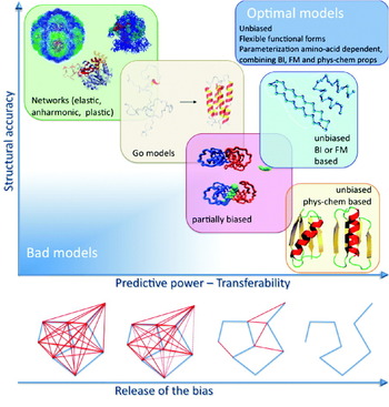
The advantages of using minimalist models are obtained at the cost of a number of emerging problems in the parameterization. Combining accuracy and predictive power in a few parameters reveals a hard task that has been faced with different strategies (Tozzini & McCammon, Reference Tozzini, McCammon and Voth2008; Tozzini, Reference Tozzini2010), giving rise to a variety of different models and parameterization recipes. In this paper, these are reviewed and classified according to the number and location of the beads, the type and form of the FF terms, and the parameterization strategy. Some technicalities and subtleties underling specific parameterization methods are particularly addressed, with the aim of including these methods within a rigorous theoretical frame. The performances and applicability of different models are also compared, and criticalities outlined. Advantages and disadvantages of the parameterization method emerge, together with regularities in the relationship between FF terms and parameters values. Overall, this analysis outlines a possible global strategy to build an optimal minimalist model and systematically assign the parameters values, which is illustrated with the aid of a schematic phase diagram for polypeptides in the parameters space.
2. Models description and FF terms
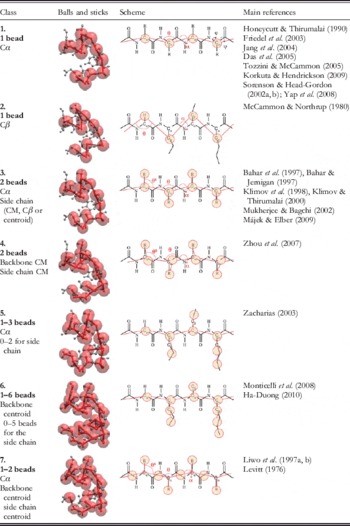
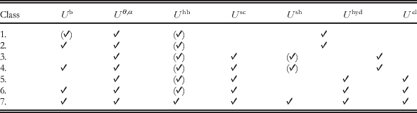
A list of representative minimalist models is reported in Table 1, separated in classes according to the number and location of the beads. Class 1 includes the most natural models, i.e. those representing an amino acid with a single interacting center (bead) placed on the alpha carbon (Cα). This representation has several advantages. First, it matches exactly with the low-resolution structural data that usually resolve only the coordinates of the Cαs, allowing for a direct data exchange with experiment (Trylska et al. Reference Trylska, Tozzini and McCammon2005). This is particularly important when one adopts a parameterization strategy based on statistical sets of structures, as it will be clear in section 4. In addition, due to rigid geometry of the peptide bond, the position of the backbone atoms is determined by the Cα coordinates, allowing the AA reconstruction of the backbone itself. This is not generally true if the bead is placed on different locations.
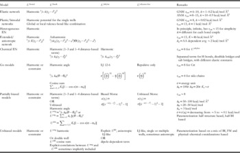
Classification of the minimalist models for proteins according to their component beads. The main internal variables are indicated in the third column. The main references are indicated. CM, center of mass

The number of internal variables is extremely reduced: only the angle θi between three subsequent Cαs and the dihedral αi between four subsequent Cαs (see Table 1 for the definitions) are sufficient to describe the conformation, since – with a few exceptions (pre-proline and cis-conformation bonds) – the Cα—Cα pseudo-bond has a value that is fixed at 3·8 Å independent of the secondary structure. As a consequence, the FF can have a very simple form

(sums over subscripts are implied), where U bond is the term describing the pseudo-peptide bond energy (often substituted with a constraint), U back describes the conformational energy and U nb the non-bonded interactions. The latter term in OB models must include very many different effects: the hydrogen bonding, the excluded volume and hydrophobicity interactions, and the electrostatics. Consequently, it can be very complex and it is often separated in sub-terms describing each effect. For instance, the excluded volume interaction is intrinsically non-isotropic, because the Cα is not located in the center of the amino acid. Models in class 2, i.e. those with the bead placed on the Cβ (or on the ‘centroid’ of the amino acid), were proposed to reduce this problem, and possess a more isotropic excluded volume term. However, additional problems arise related to the more difficult physical interpretation of the internal variables and backbone reconstruction. Related to this, the equilibrium value of the Cβ—Cβ pseudo-bond distance is no more structure independent and, consequently, the term U bond(r i,i+1) is complex and dependent on the secondary structure and amino acid type. This is true for all the models (even multiple bead models) where the backbone description is not based on the Cα positions (e.g. classes 4 and 6).
Adding one or more beads located on the side chains (classes 3–6) allow us to more easily describe the non-bonded interactions separating the side chain effects and simplify the functional form of the corresponding FF terms, although of course their number increases, including also new conformational terms (i.e. those depending on the side chain bond angles θs)

The hydrogen bond interactions of the backbone U hb(rij) are usually separated from the other non-bonded interactions, associated with the side chain beads and included in the term U nb(r sij), which is possibly decomposed in its excluded volume, hydrophobicity and electrostatic components (see also Table 2). In these models, the description of the non-bonded interactions is simpler (more isotropic, simpler functional forms), at the expense of increasing significantly the number of parameters.
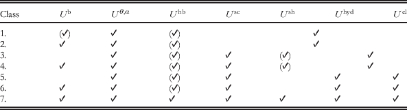
FF terms present in the different classes of minimalist models. In addition to the FF terms defined in the main text, here the non-bonded interaction for the side chain is split into its components  , where Ush describes the hydrogen bonds of the side chains, Uel the electrostatic interactions and Uhyd the hydrophobicity and excluded volume interactions, usually not separable. Optional terms are enclosed in parentheses. In classes where certain FF terms are usually treated together, the corresponding table cells are merged
Additional auxiliary beads whose position is constrained to that of the Cα and that do not increase the number of degrees of freedom are used in models of class 7 to simplify the description of hydrogen bonding and other non-bonded interactions. This class includes together one of the more sophisticated (and complex) CG models currently available (UNRES; Liwo et al. Reference Liwo, Oldziej, Pincus, Wawak, Rackowsky and Scheraga1997a, Reference Liwo, Pincus, Wawak, Rackowsky, Oldziej and Scheragab) and one of the first CG models ever reported (Levitt, Reference Levitt1976), to which most of the current ones are inspired.
Of course, a large variety of other models were considered, using up to five beads for the backbone and multiple beads representations for the side chain. This paper focuses specifically on the OB Cα-based models (class 1) and those sharing with them a similar description of the backbone conformation (classes 3, 5 and 7). A scheme of the FF terms commonly present in the different classes of models is reported in Table 2.
3. Backbone conformation description and secondary structures representability
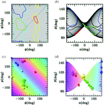
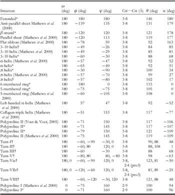
For the AA representations, a very powerful tool exists to validate the backbone conformation of a protein model: the Ramachandran plot (RP), i.e. a two-dimensional (2D) density distribution as a function of the two internal conformational variables, the pair of dihedrals (ɸ,ψ) around the two rotational bonds Cα—N and Cα—C (see Table 1, first row, third column for the definitions of dihedrals). The RP displays densely populated areas corresponding to the main secondary structures (see Fig. 1a, colored contours) in which the (ɸ,ψ) pairs assume typical values reported in Table 3, while areas outside the contours are sterically forbidden. To validate a protein model, the protein RP must not display anomalies, such as points in the forbidden areas.
Illustration of the (ɸ,ψ)→(θ,α) mapping. (a) The RP for the generic amino acid: the colored lines enclose areas where (ɸ,ψ) couples belonging to defined secondary structures accumulate: blue=extended, green=right-handed helices, red=left-handed helices. Cyan and yellow lines enclose the weakly allowed regions; other areas are sterically forbidden. (b) The (ɸ,ψ) plane is mapped in the butterfly-shaped region of the (θ,α) plot. Shades of grey show the dishomogeneity introduced by the mapping. The colored lines are the images of the profiles in (a) mapped in the (α,θ) plane, and enclose the areas corresponding to specific secondary structures, as in (a). The black lines have the same meaning, but evaluated for glycine instead of for the generic amino acid. (c) and (d): The same as (a) and (b), with the following variants: the (ɸ,ψ) plane is colored in strips at constant (ɸ+ψ) value and the color is conserved upon mapping in the (α,θ) plane. The dots represent specific kinds of secondary structures (those reported in Table 3) with the following color code: blue=extended; cyan=flat ribbon; green=right-handed helices, red=left-handed helices; magenta=proline helices; yellow=rings. In (d), the open dots correspond to directly measured data (reported in Table 3), the filled dots are obtained from the analytic mapping of the corresponding dots in the (ɸ,ψ) plane. The discrepancy is due to the use of the simplified formula for the analytic mapping (see Tozzini et al. Reference Tozzini, Rocchia and McCammon2006).

Conformational backbone variables in the most common secondary structures. The θ and α values were from the structures built with InsightII. The same software was used to build the turns using the data for (ɸ,ψ). In this case the extremal residues were added in extended conformation. For the conformations whose secondary structure is not uniform (turns) or contains peptide bonds in cis conformation the (ɸ,ψ)→(θ,α) mapping represented in Fig. 1 does not apply. (pro3) in turns VI means that the third residue is proline

* Ideal conformation as automatically built by InsightII software.
Obviously, the RP cannot be used in the class of models considered in this paper, whose internal conformational variables are (α,θ). However, the chemical constraints introduced by the peptide bond allow deriving an analytical form for the (ɸ,ψ)→(α,θ) mapping (Tozzini et al. Reference Tozzini, Rocchia and McCammon2006). Under some simplifying conditions, this is described by the following equations:
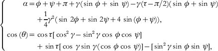
where τ=111° is the NH—Cα—CO angle and γ~16° is the angle formed by the Cα—Cα pseudo-bond and the NH—Cα and Cα—CO bonds (Tozzini et al. Reference Tozzini, Rocchia and McCammon2006). The (ɸ,ψ)→(α,θ) mapping is graphically represented in Fig. 1a, b. A uniform density in the (ɸ,ψ) plane is mapped onto a non-uniform butterfly-shaped image in the (α,θ) plane. As an effect of the mapping, the allowed areas corresponding to secondary structures are re-shaped and re-sized, as shown in Fig. 1b. The (ɸ,ψ)→(α,θ) mapping is not one-to-one: couples of points symmetric with respect to the main diagonal are mapped onto the same (α,θ) point. However, due to the specific relative location of the forbidden and allowed secondary structure areas in the (ɸ,ψ) plane, these remain separated even in the (α,θ) plane. This point is very important, because it is precisely what makes the OB–CG representation meaningful and useful to describe the secondary structures: although an (α,θ) pair corresponds to two (ɸ,ψ) pairs, only one of them falls out of the forbidden areas. Consequently, the backbone conformation is uniquely determined for each (α,θ) couple and the AA backbone conformation can be uniquely reconstructed from the CG one.
Figure 1c, d report the same information, but described in a different way. The color is conserved in the (ɸ,ψ)→(α,θ) mapping; thus the comparison of (c) to (d) shows that lines parallel to the secondary diagonal in (ɸ,ψ) are mapped in almost vertical lines in (α,θ). In addition, the color is assigned according to the ‘helicity’ of the secondary structure, changing from almost flat structures (blue to cyan) to positive (green, right-handed helices), to zero (yellow, flat rings), to negative (red, left-handed helices). Dots with the same color coding are placed in correspondence to typical values of (ɸ,ψ) for the different secondary structures reported in Table 3. In the (α,θ) plane, the colored strips become almost vertical (compare (c) to (d)), indicating that the helicity depends only on α, being ~180 for the flat structures and decreasing for helices toward the rings (α=0). Right- and left-handed helices differ by the sign of α. The (α,θ) representation of the secondary structures helicity is rather intuitive. This is evident in the (α,θ) plot for glycine, the un-chiral amino acid (black contour in Fig. 1b) for which the complete symmetry with respect to α is recovered.
In the next sections, the role of the (α,θ) plot in validating the CG models and in helping their parameterization will be clear. It is to be remarked that building a unique AA→CG mapping was possible due to the choice of the Cα as the interacting site: other choices produce more complex and secondary-structure-dependent mappings.
4. Parameterization philosophies
The minimalist CG models may have ~10–100 parameters, including both the ‘structural parameters’ (equilibrium values of the coordinates) and the ‘energetic parameters’ (elastic constants, bonding energies, well depths, barriers, etc.). There are several possible strategies to fix their values that are described in this section. To some extent, the parameterization strategy is related to the type of model, defined by the kind and number of bonded terms in the FF (the ‘topology’), their functional form and the number and functional form of the non-bonded terms. In the following, the CG models are classified and described, restricting to the OB Cα-based ones, unless otherwise stated.
4.1 Bias and fixed topology: networks and Go-models
The simplest idea to fix the structural parameters is to completely bias them toward a reference structure, usually experimental. The general form of the FF for this kind of models is

The presence and form of the terms depend on the specific model. The separation into local and non-local parts of U nb(rij) is generally based on a cutoff radius r cut: all the distances rij less than r cut in the reference structure are treated as local, the others as non-local and the corresponding FF terms are treated in different ways. In the simplest possible biased model, namely the elastic network (EN), the U nb,non-loc is absent and U nb,loc is treated with a harmonic distance-dependent potential. U back is also absent, and the correct backbone conformation is maintained by U nb,loc, which also includes the interaction between second and third neighbors along the polypeptide chain (1–3 and 1–4 interactions, equivalent of the pseudo-bond-angle and dihedral interactions, respectively). In the original formulation (Tirion, Reference Tirion1996), all the elastic constants are set at the same value k, optimized by fitting the calculated root mean-squared fluctuations (RMSF) onto the experimental temperature B factors. This fit creates an inter-dependence between k and r cut: increasing r cut, k must be softened with the rule kr cut2~cost. In subsequent works, the rule ‘the larger the cutoff, the softer the interaction’ was confirmed (Atilgan et al. Reference Atilgan, Durell, Jernigan, Demirel, Keskin and Bahar2001; Soheilifard et al. Reference Soheilifard, Makarov and Rodin2008) although the quantitative relationship does not seem to be so simple. Average values of k and r cut2 are given in Table 4.
Summary of the features of the minimalist models for proteins

Thanks to its simplicity and robustness, EN models had a great success. Under certain assumptions on the distribution of the fluctuations (the Gaussian network model, GNM, and its anisotropic version ANM; Atilgan et al. Reference Atilgan, Durell, Jernigan, Demirel, Keskin and Bahar2001; Soheilifard et al. Reference Soheilifard, Makarov and Rodin2008), they can be analytically solved, and normal mode analysis (NMA) easily performed. The low-frequency normal modes obtained from EN are seen to catch the fundamental motions of the system related to its biological function, in spite of the extreme simplification of the representation. This indicates that the connectivity and shape of a protein, namely the input of EN models, and not the structure details, generally determine its biological function. Similar information can also be obtained from the principal mode analysis (PMA) (Van Aalten et al. Reference Van Aalten, De Groot, Findlay, Berendsen and Amadei1997) of an MD trajectory, whose output are the modes ordered by amplitude. Within the harmonic approximation, the first modes (i.e. largest in amplitude) coincide with the slowest if the trajectory is equilibrated. Thus NMA and PMA give similar results once the correspondence between modes is done, but PMA uses, as input, a trajectory and does not need an analytical description of the model and thus it has a more general applicability. These analyses can be used for several purposes. The deformations associated with the slowest modes were used to flexibly fit high-resolution structural data into low-resolution electronic maps (Florence Tama & Brooks, Reference Florence Tama and Brooks2005) or to decompose the system into domains (Kundu et al. Reference Kundu, Sorensen and Phillips2004). More in general, the equilibrium dynamics of huge systems such as entire viruses was analyzed with EN models (Chennubhotla et al. Reference Chennubhotla, Rader, Lee-Wei Yang and Bahar2005; Demirel & Keskin, Reference Demirel and Keskin2005).
The limitation of these models stems from their simplicity: the bonding connectivity fixed to that of the reference structure and the use of a single-well harmonic potential constrains the system to move in the attraction basin of the reference structure, which is the only one possible equilibrium configuration. In addition, the use of a unique elastic constant for all the possible, bonded and non-bonded interactions of the system is clearly a un-physical oversimplification. Thus improved network models were proposed that release one or more of these restrains. Plastic networks (Maragakis & Karplus, Reference Maragakis and Karplus2005) and multiple-well networks (Chu & Voth, Reference Chu and Voth2007) allow studying systems with two or more equilibrium conformations. Each conformation is represented with an EN model, subsequently coupled with a valence-bond-like approach. For instance, in the case of two states A and B

where U A and U B refer to the single states and the combination can be done either at the global level (i.e. U A,B are the total potential energies; Maragakis & Karplus, Reference Maragakis and Karplus2005) or at the local level (i.e. U A,B=u AB(rij) are the single pair potentials; Chu & Voth, Reference Chu and Voth2007). In both cases, the standard EN parameters are used for the single well, but additional parameters are needed: the coupling parameter ε and the relative free energy of the two states. These models are able to describe the transition between two known structural states, to find the minimum free energy paths and analyze the properties of the system along them.
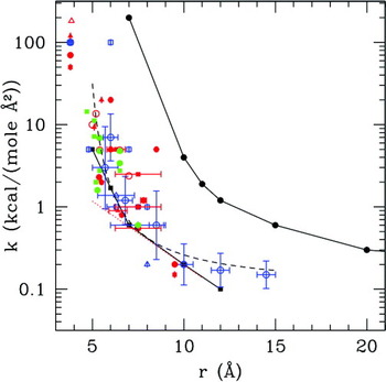
Heterogeneous EN (Lyman et al. Reference Lyman, Pfaendtner and Voth2008) models were proposed to improve the quality of the RMSF. In these models, k is not uniform: conversely, kij for each single interacting pair is considered a fitting parameter. Clearly, there is the need for a large amount of input data, for such a large number of fitting parameters; that is why these models usually take as input the RMSF evaluated over different normal modes of the system from AA simulations. As a result, normal mode displacements and RMSF of the CG model will have good agreement with those of the AA model. The elastic constant strength as a function of the equilibrium distance is obtained as a by-product, and it is decreasing (Fig. 5), in agreement with the intuitive consideration that shorter interactions are stronger. Elastic constants dependent on the amino acids type were introduced in the ‘extended’ ANM, where also an anharmonic potential for the non-subsequent Cα pairs was used (Hamacher & McCammon, Reference Hamacher and McCammon2006). The ks were obtained based on available statistical contact potential matrices (Keskin et al. Reference Keskin, Bahar, Badretdinov, Ptitsyn and Jernigan1998; Miyazawa & Jernigan, Reference Miyazawa and Jernigan1996) readjusted on the experimental RMSF. This model gives better-quality RMSFs and accounts for the effect of mutations.
The simplicity of EN is obtained at the cost of the need for a large number of contacts for each bead for the system to be stable, scaling approximately with r cut3. In order to reduce the computational cost and with the aim of having more physical FF terms, ENs with physics/chemistry-based topology were proposed. In the ‘chemical network’ (Jeong et al. Reference Jeong, Jang and Kim2005), the FF terms are separated according to amino acid type with different ks calibrated fitting the overlap of displacements from the NMA. As a consequence, r cut can be greatly reduced without losing stability and accuracy.
The Go models belong to the class of biased models, although their purpose, FF terms and parameterization philosophy differ from those of EN. Originally proposed as a simplified statistical model for folding (Go & Scheraga, Reference Go and Scheraga1976), more recent versions (Clementi et al. Reference Clementi, Nymeyer and Onuchic2000; Koga & Takada, Reference Koga and Takada2001) include terms with a more physical form than EN. U bond is the usual harmonic term, while U back depends on the backbone conformational variables θ and α, and is separated into the corresponding two terms (usually harmonic and cosine series, respectively). The r cut in this case has the meaning of separating the couples of amino acids that are in contact in the folded structure (called the native contacts) from the others. The U nb,loc acting between pairs in native contact is represented as an attractive Lennard–Jones (LJ)-like potential, while the U nb,non-loc is repulsive, so as to push the system toward the native conformation. This form of Go model is also called the minimally frustrated model for folding, because the local minima other than the native structure are almost absent. The elastic constants and other energetic parameters are fixed to be proportional to ε, the LJ well depth (see Table 4). Thus, the energetic properties of the system are entirely determined by a single parameter, ε, which is adjusted to fit the experimental melting temperature. The philosophy underlying these models relies on the assumption that the native structure (the main input of the model) determines the folding pathway and other global properties of the folding process. However, this is true only in the first approximation: by construction, and due to the absence of frustration, the Go model fails to catch the nature of the intermediate states that often occurs during folding. For these reasons, the evolutions of the Go model have followed the direction of including frustration, either in U back (Nakagawa & Peyrard, Reference Nakagawa and Peyrard2006) or in U nb (Kaya & Chan, Reference Kaya and Chan2003).
4.2 The Boltzmann inversion
The bias toward a single structure is the main limit of the network and Go models, which, although very useful in describing the near equilibrium dynamics or the global properties of folding, are inadequate to describe more general dynamical properties. A possible way to overcome this limit is to extract the parameters from a statistical set of structures. As it will be clear in the following, the origin of the structures (e.g. experimental or from AA simulations) may influence the features of the FF.
A possibility to extract parameters from a statistical set of data is the Boltzmann inversion (BI). Suppose that the total internal energy of the system can be exactly decomposed as the sum of uncorrelated terms, each depending on a single internal CG variable, i.e.
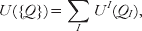
where UI=U bond, U angle, etc. and QI=ri,i +1, αi, etc. ({Q} indicates the whole set of coordinates). The probability distribution of a single internal variable is

and the second equality stands if the condition of complete un-correlation between the FF terms is valid. This condition is never exactly satisfied, especially in the case of the OB FFs. The consequences of this approximation will be illustrated later on. Equation (4.4)) is equivalent to

that defines the core of the BI, and gives an operative way to derive the CG FF terms based on the probability distribution of internal variable, which can be evaluated given a statistical set of structures.
4.2.1 The Boltzmann inverses (BIns) of the conformational internal variables
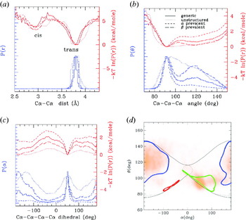
In order to give an idea of how the BIns look like, those for the three conformational internal variables (Cα—Cα distance, pseudo-bond-angle θ and pseudo-dihedral α) are reported in Fig. 2. The probability distributions for three different sets of proteins and the corresponding BIn are shown. The pseudo-bond distribution (BIn) is bimodal, but the position of the peaks (minima) is independent of the secondary structure: rather they correspond to the trans and (rare) cis conformation of the peptide bond. The independence of the secondary structure is related to the fact that Cαs were chosen as the location for the interacting centers. Conversely, the multiple peaks in the pseudo-bond distributions for models with beads placed on Cβ or centroids (e.g. classes 2 and 4) are signatures of the secondary structure (Monticelli et al. Reference Monticelli, Kandasamy, Periole, Larson, Tieleman and Marrink2008).
Probability distribution of the internal variables evaluated using different statistical sets: 102 large proteins (size ~50 Å, solid line); 312 proteins with prevalence of β-strands (long dashed line); 347 proteins with prevalence of α-helices (short dashed line); 450 proteins prevalently unstructured (dotted line). The sets were prepared with the selection tools of the RCSB databank website (RCSB protein databank, http://www.pdb.org/pdb/home/home.do). Blue lines: arbitrarily normalized variable distributions; red lines: BIn, units on the right-hand vertical axis. (a) First neighbor distance distributions; (b) pseudo-bond-angle distributions; (c) pseudo-dihedral distributions; (d) the (α,θ) plot for the set of generic proteins (in orange), superimposed on the ideal map (see also Fig. 1).

The probability distributions of θ and α (and BIn) also display multiple peaks (minima), and these correspond to different secondary structures of both Cα-based and non-Cα-based models. However, in Cα-based models the relation between peaks and secondary structures is more direct, as explained in section 3. More specifically, P(θ) displays a peak at ~90° typical of the α-helices, while the β-like structures have θ=115–145 depending on the kind of amino acid. Figure 2b clearly shows how the relative population of the two peaks varies passing from a α-prevalent to β-prevalent set of proteins, while in the mainly unstructured proteins the two peaks are broader. Similar consideration can be done for the α pseudo-dihedral distributions, where the peak typical of helices is located at ~60°, while the extended structures tend to adopt a value of ~178°. In Fig. 2d, the correlation (α,θ) plot is also reported for the set of generic proteins, which shows a good superposition with the ideal (α,θ) plot (see section 3).
4.2.2 BIns and potential of mean forces (PMFs)
The BIn from eqn (4.5) is often identified with the PMF. However, rigorously speaking, they are not exactly the same, although their difference is seldom clearly stated (Májek & Elber, Reference Májek and Elber2009). The PMF is defined by
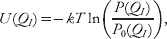
where P 0(QI) is the probability distribution of the internal variable in a reference state, usually the system with non-interacting particles (but the choice of the reference state is a matter of debate (Betancourt & Thirumalai, Reference Betancourt and Thirumalai1999). Non-interacting particles distribute randomly in the 3D space; thus P 0(QI) is usually constant and the PMF differs from the BIn by an irrelevant constant. However, in certain specific cases, this is not true. For instance, consider QI=θ: the P 0 distribution of uniformly distributed points on a sphere is not uniform, but rather P 0(θ)∝sin(θ), due to the fact that the lateral surface of a spherical horizontal section increases with sin(θ). Thus, in this case, one has that PMF is U(θ)=−kT ln [P(θ)/sin(θ)]. This correction is usually neglected because sin(θ) varies only ~20% from the α peak to the β peak.
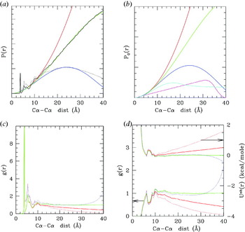
In other cases, however, the correction is relevant and the difference between BIn and PMF is substantial. Consider, for instance, the probability distribution of distances between any two pairs of Cα, P(r), which is related – after some elaboration (see the following section) – to the non-bonded interaction potential. For an infinite system of non-interacting particles, one has P 0(r)=4πr 2, that is, the volume of the spherical shell of radius r, to which also P(r) should tend for large r. Thus the PMF is U(r)=−kT ln (P(r)/4πr 2)=−kT ln(g(r)), where g(r) is the pair correlation function. Figure 3 illustrates the differences between the mentioned quantities with practical examples. In (a), the P(r) is shown (black lines). As it can be seen, however, for r>10 Å its behavior strongly deviates from 4πr 2 (red line). This is due to the fact that the proteins have finite size; thus their P(r) vanishes for r larger than the average protein size. Thus, in this case, P 0(r) should be the distribution of non-interacting particles limited in a sphere of finite radius (R), which can be analytically calculated solving the integral from the definition, and is
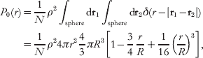
where N is the total number of beads and ρ the average particle density. This expression tends to 4πr 2 as R tends to infinity. Empirical approximations of this formula were earlier derived (Zhou & Zhou, Reference Zhou and Zhou2002). Figure 3a shows that expression eqn (4.7) reproduces the correct behavior of P(r) for large r.
(a) In black, probability distributions of the pair distances for a set of large proteins (3000–6000 residues, solid line) and for a set of small proteins (<1000 residues, dotted line). Superimposed in red are the P 0(r) evaluated for an infinite system (red) and for spherical systems (eqn (4.7)) of radius 45 Å (green) and 23 Å (blue), which best fit the P(r) for large and small proteins, respectively. The fit is worse for the small proteins set, probably due to the poor size homogeneity in this set. These P 0(r) are also reported in (b) together with that evaluated for a spherical shell of inner radius 15 Å and outer radius 20 Å (magenta) and that for an infinite cylinder of radius 11 Å (cyan), evaluated numerically. The normalizations are such that the quadratic parts for r<5 Å superimpose. (c) The pair correlation function g(r) for large (solid) and small (dotted) proteins normalized with the infinite radius P 0(r) (red) and with the finite radius (R=45 for large proteins, green, and R=23 for small proteins, blue). (d) Plots in the lower part of the graph, scale on the left vertical axis non-bonded parts of g(r), the same color and line code as in (b); Plots in the upper part of the graph, right vertical axis: the corresponding PMF, the same color and line codes.

In Fig. 3b, the P 0(r) for a spherical shell of inner radius 15 Å and outer radius 20 Å is shown in magenta and that for an infinite cylinder of radius 11 Å is shown in cyan. These P 0(r) values are relevant when dealing with a viral capsid and with DNA, respectively. The behavior is quadratic within the thickness of the shell or of the cylinder and then becomes linear for the shell and tends to a constant for the cylinder. In general, P 0(r) with the same global geometry of the system that one is analyzing should be used, if the correct long-range behavior of the pair g(r) is to be evaluated. As it can be seen in Fig. 3c the g(r) tends to 1 only if the correct P 0 is used (green and blue lines). This reflects in the long-range behavior of the PMF: in Fig. 3d, the g(r) and the corresponding PMF are shown. Different lines correspond to different P 0. Only using the correct P 0(r) one obtains the correct asymptotic vanishing behavior of the PMF.
4.2.3 From the PMF to the effective interactions
The concept of PMF gives an operative way to build the FF terms: under certain approximations, the PMFs could be used either directly (in numerical form) as FF terms or to fit the parameters for corresponding analytical FF terms. For instance, from distributions and PMFs such as those in Fig. 2a, the U bond term can be fitted with a simple harmonic form with r 0=3·8 Å or 2·9 Å and k~100–150 kcal/mol; the bond angle and dihedral terms need more complicated analytical forms, but both the equilibrium and energetic parameters can in principle be extracted from the PMFs.
Unfortunately, this view is fairly too optimistic. This procedure cannot be straightforwardly applied for at least three reasons: (i) the probability distributions depend on the amino acid type; thus in order to have an accurate FF, one should build ~202 different PMFs for the P(r), ~203 for P(θ) and 204 for P(α); (ii) the probability distributions (and the PMFs) depend on the statistical set chosen; (iii) the internal variables chosen are not uncorrelated; thus eqn (4.3) is not exact and the PMFs do not coincide with the real effective interaction potentials (i.e. the FF term).
Issue (i) is not a problem in principle, but the large number of probability distributions to build, possibly with similar occurrence statistics (which is difficult because different amino acids have different occurrence frequencies), has limited the use of the method, at least exclusively. However, several CG FFs have some of the terms, especially the bonded ones, directly determined by BI of the corresponding distributions (Bahar & Jernigan, Reference Bahar and Jernigan1997; Bahar et al. Reference Bahar, Kaplan and Jernigan1997; Monticelli et al. Reference Monticelli, Kandasamy, Periole, Larson, Tieleman and Marrink2008; Tozzini & McCammon, Reference Tozzini, McCammon and Voth2008).
Issue (ii) points out an interesting problem: the probability distribution depends on the statistical set chosen. In particular, the relative amount of helical versus extended secondary structures influences the bonded terms distributions (see Fig. 2b, c) and the short-range part of the non-bonded one, as it will be clear further on in this section. Some author (e.g. Monticelli et al. (Reference Monticelli, Kandasamy, Periole, Larson, Tieleman and Marrink2008)) have turned around this problem by using FFs bonded terms depending directly on the secondary structure (that must be a priori known) rather than on the amino acid type. In addition, the probability distributions also depend on the origin of the data. Data from AA simulations usually span a limited area of the conformational space, due to the limited AA MD run lengths, meaning that the structures in the set are generally less structurally diverse than in an experimental data set. For this reason, the peaks present in the distributions from simulations tend to be sharper and better defined, generally leading to larger energetic parameters. However, using parameters generated from AA simulation turns out to be useful especially in multi-scale simulations, where compatibility with AA simulations is required (Zhou et al. Reference Zhou, Thorpe, Izvekov and Voth2007).
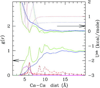
However, issue (iii), the correlation between FF terms, is the main reason that prevents using the simple PMFs as effective CG interactions. This concept will be illustrated by means of a deeper analysis of the non-bonded part of the distance probability distribution, whose PMF is related to U nb(r). Figure 4 shows the g(r) and corresponding PMFs, evaluated using a set of proteins with natural statistical occurrence of helical and sheets structures. The green line is the ‘non-bonded’ g(r), obtained excluding from the distribution the first, second and third neighbors along the polypeptide chain, which are related to the U bond and U back terms. One would, in principle, expect that the PMF from this g(r) has an LJ-like shape. However, Fig. 4 (green lines, upper plot) shows that it is far from being a single well van der Waals (vdW)-like potential, rather it is multi-welled. For instance, the more evident peak at ~6·2 Å corresponds to the distribution of the fourth neighbors (1–5 neighbors, red solid line): the Cα separated by four amino acids along the chain assume quite sharply that distance when they are in helical conformation. Thus that peak can be thought as due to the presence of the hydrogen bonds that maintain stable the helix. Other peaks at ~8·5, ~10, 11 and 14 Å, present in the fifth to tenth neighbor distribution (dashed red line), have a similar origin: they are due to the regular recurrence of distances in the helical structure. Here the concept of ‘correlation’ emerges: while the first peak (well) at 6·2 Å can be put in relationship with the presence of an additional interaction term in the FF (e.g. the hydrogen bond U hb), the additional peaks (wells) in the g(r) (PMF) are not due to additional terms, but are induced by U hb via multi-body correlations present along the helical structures. Similarly, the backbone hydrogen bonds among strands in a sheet are responsible for the three overlapping peaks at ~4·5, 5·0 and 5·5 Å (magenta line), and only these, not the corresponding induced peaks, should be included as explicit terms in the FF.
Non-bonded part of the pair correlation functions (lower plots, left-hand vertical axis) and the corresponding PMF (upper plot, right-hand vertical axis). Color codes: green=total non-bonded g(r) obtained excluding the first, second and third neighbors along the polypeptide chain (that pertain to pseudo-bond, pseudo-bond-angle and pseudo-dihedral distributions); red solid=g(r) for the 1–5 distances (fourth neighbors along the polypeptide chain); red-dashed=g(r) for the 1–6 to 1–10 distances; magenta=g(r) of the distances of Cαs involved in hydrogen bonds between strands in sheets; blue=green minus red and magenta (i.e. ‘real’ non-bonded part). The distribution of hydrogen bonds in the sheets is obtained with the following criteria: the two Cαs i and j are considered to form a hydrogen bond in a sheet if also (i+1, j−1) and (i−1, j+1) (anti-parallel sheet) or (i+1, j+1) and (i−1, j−1) (anti-parallel sheet) form a hydrogen bond. Dotted lines on the upper graph are fits to the minima with Morse functions (f(r)=ε[(exp(−κ(r−r 0))−1)2−1]), which have an additional parameter κ with respect to LJ potential related to the width of the well. The Morse potential turns out to be more appropriate given the variably softer nature of the CG non-bonded interactions. The statistical set used is the set of ‘small proteins’ as in Fig. 3.

Once all the U hb (and their correlated) are subtracted, only the excluded volume, hydrophobic and electrostatic interactions remain. The corresponding g(r) and PMF look much smoother (blue lines) although a couple of structures at ~6 and ~10 Å are still visible (even more evident in the amino-acid-specific distributions (Trovato & Tozzini, Reference Trovato and Tozziniin preparation), thought to be due to other factors: intrinsic anisotropy of the excluded volume side chain interactions, hydrophobic interactions mediated by water molecules, etc. Thus these distributions (blue lines), and not the original g(r) (green lines), should be used to parameterize the U nb term.
The one described above is an empirical way to separate the ‘genuine’ FF terms from the peaks due to correlations in the PMF. However, a rigorous way to generate a ‘true’ effective potential from PMF exists that, in principle, does not require any arbitrary choice. This is the Iterative Boltzmann Inversion (IBI) (Reith et al. Reference Reith, Pütz and Müller-Plathe2003). It consists in using the g(r) as the target function to be reproduced iteratively proceeding as follows: (1) use the PMF as initial guess for Ui(r) and generate a gi(r) from a simulation; (2) correct the Ui(r) with the formula
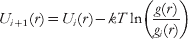
and repeat step 1 with Ui +1(r). At convergence, this procedure gives the effective potential that best reproduces the target g(r) and, in principle, should be applied to determine each term of the FF at the same time (using the corresponding probability distributions as targets). In practice, however, as the number of terms increase, a number of problems arise. Even assuming that the simple BI (not iterative) is enough for the bonded terms (less affected by the correlation problem), and restricting the IBI to U nb, one should apply it to ~202 different terms. In addition, in order to obtain a general and transferable potential, the simulations should be performed not on a single structure, but on a set of diverse representative structures. For these reasons, the IBI is only rarely applied to biopolymers (Májek & Elber, Reference Májek and Elber2009) and usually in simplified forms (Banachowicz et al. Reference Banachowicz, Gapinski and Patkowski2000).
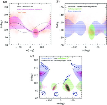
As previously noted, it is sometimes assumed that the bonded terms of the FF are less affected by the problem of correlations, but this is not entirely true. Observing Fig. 2d it is apparent that P(θ) and P(α) are not independent, rather certain values of α and θ appear preferentially in a correlated way, for instance θ~90° and α~60° in the helices. These correlations can be seen as induced by the presence of additional terms of the FF: specifically the θ~90, α~60 can be seen as induced by the hydrogen bond terms that stabilize the helices. This again points out the necessity of taking with great care the direct BIn as the interaction potential, even in the case of the conformational terms.
4.2.4 Examples of models based on BI
In spite of these problems, many CG FF are at least partially based on BI, using a simplified version of the iterative approach. Among these, there are the partially biased models, first introduced to simulate the large-scale dynamics of the HIV-1 protease (Tozzini & McCammon, Reference Tozzini and McCammon2005; Tozzini et al. Reference Tozzini, Trylska, Chang and McCammon2007) and subsequently applied also to larger systems such as the ribosome (Trylska et al. Reference Trylska, Tozzini and McCammon2005), nucleosomes (Voltz et al. Reference Voltz, Trylska, Tozzini, Kurkal-Siebert, Langowski and Smith2008) and viruses (Arcangeli & Tozzini, Reference Arcangeli and Tozziniin preparation). In these models, the FF form is as in eqn (4.1)), with the U back conformational term separated in U ang and U dih. The philosophy underlying these models is to gradually abandon the bias toward a reference structure and base the parameterization on the unbiased terms on BI. Particular attention is devoted to the functional form of the unbiased terms, such as U ang, which in Tozzini & McCammon (Reference Tozzini and McCammon2005) is represented with a double-well quartic potential

where θ0 is the location of the first well (~90°), and the other parameters are amino acid type dependent and determine the position of the second well and its relative stability. The parameters are extracted from the direct BIn (or PMFs) either from experimental structures (in Tozzini et al. (Reference Tozzini, Trylska, Chang and McCammon2007) and Trylska et al. (Reference Trylska, Tozzini and McCammon2005)) or from AA simulations (in Voltz et al. (Reference Voltz, Trylska, Tozzini, Kurkal-Siebert, Langowski and Smith2008)) and then optimized using the probability distributions as targets. U nb, both local and non-local, is represented with a Morse potential, but a partial bias is conserved in the structural parameters of U nb‐local: the equilibrium distances r 0ij differ for each ij couple and are taken from a single reference structure. The distinction between U nb–local and U nb–non-local is similar to that in EN and Go models, but both the parameters and the cutoff are based on physical grounds: looking at Fig. 4, the cutoff can be naturally placed at ~8 Å, which separates the local part of U nb, containing mainly the hydrogen bond interactions, from the non-local, less structured part, containing mainly the hydrophobic and electrostatic interactions. Thus the local bias allows us to represent in a very simple way the most complex terms of the FF, maintains the structure stable and gives a high level of structural accuracy that allows these CG models to be compatible with AA models in multi-scale approaches (Chang et al. Reference Chang, Trylska, Tozzini and McCammon2007). At the same time, the other unbiased terms give enough flexibility to the system, so that even out of equilibrium dynamics can be simulated, such as the substrate capture process of HIV-1 protease (Trylska et al. Reference Trylska, Tozzini, Chang and McCammon2007) or the allosteric motions upon binding of HIV-1 integrase with HAT proteins (Di Fenza et al. Reference Di Fenza, Rocchia and Tozzini2009).
A similar approach was adopted to build the VAMM FF (Korkuta & Hendrickson, Reference Korkuta and Hendrickson2009). The FF terms are the same (eqn 4.1) and the parameterization based on BI, with more complex functional forms for U ang and U dih. At variance with Tozzini et al. (Reference Tozzini, Trylska, Chang and McCammon2007), parameterization of these terms is secondary structure dependent instead of amino acid type dependent, to improve the structural accuracy, although a priori knowledge of the secondary structure is required. U nb–local is biased toward a reference structure, but at variance with Tozzini et al. (Reference Tozzini, Trylska, Chang and McCammon2007), the local–non-local separation is based on the distance along the chain (j–i<6) instead of on a distance cutoff. This implies that a double well U nb–non-local is necessary to account for the residual short-range interactions (Fig. 4, blue dotted lines).
Although it originates as an evolution of the Go models and is specifically designed for folding, even the Das, Matysiak, Clementi (DMC) model (Das et al. Reference Das, Matysiak and Clementi2005) can be put in the class of the partially biased because in the non-bonded interaction the bias is somewhat eliminated. U bond and U back are parameterized as in the usual Go models based on a single structure. Conversely the U nb assumes the form

(it is to be observed that a 12–10 form is used instead of the usual 12–6 LJ potential, which is quite similar to the Morse form with intermediate values of the κ parameter). U nb is not separated into local and non-local parts; however, the parameters ε, δ (=0 or 1) depend on the amino acid type (ai,j), and σ depends also on the distance of i and j along the chain. Three classes are considered: j–i=4, j–i=5 and j–i>5. Thus, in some sense, the separation between local and non-local parts of the non-bonded interaction is recovered by recognizing that the 1–5 and 1–6 interactions are qualitatively different from the others. The σs are parameterized by BI of a statistical set of non-redundant proteins (Das et al. Reference Das, Matysiak and Clementi2005). The set of {ε, δ} is obtained through a complex optimization procedure that involves the minimization of the distance of the simulated folded structure from the native one, the free energy experimental differences upon mutations, and other available observables (Matysiak & Clementi, Reference Matysiak and Clementi2006). The separation into classes and the amino-acid-dependent parameters enhances the structural accuracy of the model. However, the set of parameters is protein dependent; thus the problem of transferability to different proteins is not completely solved. The DMC model improves the folding landscape characterization by improving the local structural accuracy with BI-based terms and at the same time eliminating a part of the bias present in the Go models.
As already observed, the difficulty in completely releasing the bias in OB models stems from the fact that the non-bonded interactions, especially the local ones, are very complex and highly anisotropic. Thus maintaining the local bias is a simple compromise solution to have high accuracy without introducing a large number of parameters and complex functional forms (Mukherjee et al. Reference Mukherjee, Bhimalapuram and Bagchia2005). A part of the problem, specifically that related to the anisotropy of the interactions of the side chains, is solved in the Cα-based two-bead (or multiple bead) models. Some of them are worth mentioning here although this paper is focused on the OB models, because based on BI. In the two-beads model by Bahar & Jernigan (Reference Bahar and Jernigan1997) and Bahar et al. (Reference Bahar, Kaplan and Jernigan1997), the backbone U ang and U dih terms are numerically evaluated by BI and are aminoacid type dependent. Conformational terms pertaining to the orientation of the side chain and U corr(θ,α) term are added to account for the correlations between the backbone conformational variables. The non-bonded terms between side chains are obtained with the same philosophy.
The CALF FF is virtually a two-bead model, although the position of the side chain is entirely determined from that of Cα (Buck & Bystroff, Reference Buck and Bystroff2009). From the FF form point of view, it is interesting because explicit terms for the hydrogen bonds U hb are introduced. The parameterization procedure is BI related but quite complex. Given a protein, first the local structure is determined from the local sequence, through a statistical procedure. Second, based on the local structure, the U back and U hb terms are parameterized, including statistical information through BI. This model is used for folding. Similar for the FF terms and for the philosophy of the parameter assignment (based on the local structure) is the OPUS-Ca FF (Wu et al. Reference Wu, Lu, Chen, Li and Ma2007), which uses very complex parametric forms for the FF terms. These models are quasi-unbiased, but the bias is hidden in the a priori determination of the local structure, upon which the FF is based.
The MARTINI FF, recently extended to proteins (Monticelli et al. Reference Monticelli, Kandasamy, Periole, Larson, Tieleman and Marrink2008), is a multiple bead model where the backbone bead is placed on the centroid of the NH-Cα-C=O group and 1–4 beads are used for the side chains; in addition, the solvent is explicit, although it is CG itself. Thus the level of coarse graining is not particularly extreme. However, this model is interesting for the purpose of the present paper because the choice of FF terms and parameterization contains elements that can be considered exemplar even for Cα-based models. U bond is a simple harmonic form, including in this case also the terms between Cα and the side chains. U back is split into the bond angle and dihedral part, all represented by single-well functions. Additional conformational terms are assigned to maintain the correct orientation of the side chain. U nb is split into an LJ plus a screened Coulomb part, representing excluded volume and hydrophobic interactions and electrostatic, respectively. U hb is absent: the secondary structure is maintained by the U back terms, whose values are derived based on the BI. The side chain non-bonded interaction parameters are amino acid type dependent and were optimized including thermo-statistics data from experiment (e.g. free energy of water–oil partitioning) or from AA simulations (amino-acid association constants). As for OPUS-Ca and CALF, although the bias toward a single structure is completely removed, a priori knowledge of the secondary structure is necessary. In addition, no transitions between different secondary structures are allowed.
4.3 The Force Matching (FM) method
4.3.1 Mechanical consistency versus thermodynamic consistency
The BI-based methods can be thought of as realizing the ‘thermodynamic consistency’ of the CG model with a given statistical set of data. In fact they use as the target quantity to reproduce in the CG simulations the probability distributions or, equivalently, the corresponding BIn, which are related to the internal variable-dependent free energies

where Q is a collective variable (e.g. a CG internal variable). This is the general form of eqn (4.5) valid for any kind of collective variable Q. The additive constant is equal to −kT times the logarithm of the partition function. The relation between F(Q) and the corresponding PMF is

where the subscript 0 refers to the reference system, usually the non-interacting particle system. As discussed in the previous section, PMF and the corresponding free energy differ by more than a simple constant if the choice of the variable Q is such that F 0 is not independent of it. In the previous section, it is also discussed how it is possible to obtain the ‘best’ U(Q) starting from PMF(Q) with the iterative BI.
In principle, BI could be applied also to many-body PMFs and effective potentials. One could consider a many-body CG potential depending on a set of collective CG variables {Q}

and determine it with a full convergence multi-variable IBI procedure, using a set of probability distributions P({Q}) (from experiment or from simulation) as the target. Equations (4.11) and (4.12) are valid also when Q is replaced by the set of {Q} and the corresponding multivariate quantities (probabilities, free energies, PMF) are defined. The IBI procedure then gives the effective multi-body CG potential U({Q}) that best reproduce the free energy F({Q}) of the system (i.e. the Free Energy Surface) and consequently its thermodynamic properties.
An alternative route to determine effective CG potentials is the ‘force matching’ (FM) method, targeting the reproduction of the forces (Ercolessi & Adams, Reference Ercolessi and Adams1994; Izvekov et al. Reference Izvekov, Parrinello, Burnham and Voth2004). The forces acting on the CG sites are calculated with a more accurate method (e.g. AA MD simulations) and then used as the target to fix the parameters of the CG potential or to fit a potential in numerical form. This method was rigorously formulated and optimized in a series of papers by Izvekov & Voth (Reference Izvekov and Voth2005), Wang et al. (Reference Wang, Noid, Liu and Voth2009), Noid et al. (Reference Noid, Chu, Ayton, Krishna, Izvekov, Voth, Das and Andersen2008a), Das & Andersen (Reference Das and Andersen2009) and Noid et al. (Reference Noid, Liu, Wang, Chu, Ayton, Izvekov, Andersen and Voth2008b), who named it the multi-scale CG (MS-CG) method. The basic idea is to minimize the functional

where FI are the CG forces on CG sites I, fI are the forces on the CG sites evaluated from the AA simulations, and 〈〉 represents the average along the trajectory (or within the data set) that is intended to be large enough to sample the canonical ensemble. The statistical average eliminates the explicit dependence on the AA ({q}) internal variables, so that χ2 is a functional only of the functions FI({Q}), i.e. the CG forces, to be determined by minimizing χ2. It is shown that the minimal FI({Q}) satisfies the equation
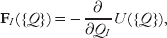
where U({Q}) is the multi-body PMF related to the P({Q}). This equation puts in relation the (I)BI with the FM methods. In practice, however, there are substantial differences between the two methods, at different levels. First of all, the input data set is typically different. The BI-based procedures take, as input, structures from any source, but preferentially experimental, to enlarge the diversity of the data set, in order to improve the transferability of the parameters. Conversely, the FM procedure needs, as inputs, the forces on CG sites that are typically evaluated along AA MD simulations. This difference in the inputs used in the two techniques results in differences in the FF terms: the FF terms from (I)BI tend to be ‘softer’ (multiple minima, larger and less defined), while those from FM tend to be ‘harder’ (sharper and better defined minima). In addition, the use of AA simulation structures as input data generates another question, which is the question related to the accuracy and reliability of AA FFs that is assumed in this approach. It is beyond the scope of this paper to analyze this problem; however, it is to be mentioned that the most commonly used AA FFs have recently revealed some inaccuracies that appear especially on the long time scale (Okur et al. Reference Okur, Strockbine, Hornak and Simmerling2003; Ono et al. Reference Ono, Nakajima, Higo and Nakamura2000). The possible differences between CG FFs generated by the use of different input data sets are coherent with the usually different use made of the BI and FM CG FFs: the former are generally used to address general dynamics in CG-only simulations, while the latter are preferentially used in multi-scale simulations, where the CG results must be compared with the AA ones. In fact, the MS-CG method is designed to realize the mechanical consistency between AA and GC models.
Even considering an identical input set of structures, different FFs may arise from the different approximations adopted in the two methods. Neither in FM nor in BI the exact multi-body U({Q}) or forces are usually considered. Rather, in both cases they are decomposed into a finite sum of terms. In the case of the (I)BI-based methods this simply corresponds to write the FF as a sum of terms depending on the single internal CG variables, i.e. eqns (4.3) or (2.2). As already discussed, behind this choice there is the assumption that the choice of the FF terms and explicit internal variables is made in such a way as to reduce at minimum the correlation between terms. The parameters of the FF terms are then varied in order to optimally reproduce the PMFs or probability distributions by direct or iterative BI, as explained in the previously.
In the case of the MS-CG method, the forces on the CG sites are expressed as a linear combination of ‘basis’ functions G({Q}):

and the coefficients ɸ are determined by variationally minimizing eqn (4.14)). The exact form of G({Q}) depends on the kind of system. For instance, if the pair-wise interactions are dominant in the system, e.g. for a one-component system formed by non-bonded elements, it becomes convenient to use the Cartesian coordinates of the CG sites and express the forces in the form

where RIJ is the pair-wise distance between two CG sites and δ(R) is a discrete delta function. This particular choice returns directly the pair-wise force acting among the components (FI({R})), assuming that multi-body forces are negligible.
It is clear that (I)BI and FM methods, although stemming from a common basis, use different inputs and different approximations. The FM method has the advantage of directly giving the effective interaction potential without the need of iterative procedures. On the other hand, the (I)BI procedure is more broadly applicable, because it needs only the structures and not the forces as input, although it needs more care and efforts to obtain accurate effective potentials.
4.3.2 Examples of FFs based on the FM
The MS-CG method was used for a variety of systems of biological interest (lipid bilayers (Izvekov & Voth, Reference Izvekov and Voth2006) with membrane proteins (Shi et al. Reference Shi, Izvekov and Voth2006), monosaccharides (Liu et al. Reference Liu, Izvekow and Voth2007). For the purposes of the present paper, it is useful to cite its use in a two-bead model of class 4 (Zhou et al. Reference Zhou, Thorpe, Izvekov and Voth2007) (see Table 1) in which the MS-CG procedure was used to model the non-bonded interactions between beads, while the direct BI is used to model the bonded interaction terms, assuming that these are slightly affected by the correlation problem. At variance with previous models, in this one the dihedral term for the backbone is omitted: the task of maintaining the correct dihedral value and backbone conformation is entirely demanded from the hydrogen bonding between backbone atoms including the non-bonded interactions between backbone beads. Referring to eqn (4.1), U back depends only on θ, while U nb−loc is completely unbiased and contains together effects of hydrogen bonding and other local interactions. It is derived in a numerical form using eqn (4.17), as far as the non-bonded potential terms for the side chains, which in this model assume the role of U nb−non-loc. This model was shown to describe properly the dynamics folding landscape of a 15-mer of poly-alanine. Conversely, to describe accurately the β-hairpin structure, an analogously derived model but with three beads for the backbone was used (Thorpe et al. Reference Thorpe, Zhou and Voth2008), due to the fact that for the β-hairpin structure, the correct conformation of the backbone hydrogen bond is critical, and this is better described using more bead for the backbone.
4.4 Physics–chemistry-based models and combinations of methods
The BI and FM methods allow, in principle, to parameterize very accurately effective potentials, once the decomposition of the FF in single terms is established. However, from the previous analysis two main problems emerge: (i) in principle, all the FF terms must be parameterized in an amino-acid-type-dependent fashion, in order for the FF to be predictive; (ii) the FF terms and their functional forms must be properly chosen. In this section, a group model is reported that tries to face and solve the problems related to (i) and (ii) including in the parameterization elements based on the known chemical and physical properties of the amino acids and/or thermodynamics and statistical data from experiment, and reducing at minimum the necessary a priori knowledge of the system. This procedure is not at all new in the field of empirical FF simulations, since even in the parameterization of the AA FFs physics- and chemistry-based elements are introduced. In addition, in this group of models the focus is moved from the reproduction of the local structure to the prediction of the global fold (secondary and tertiary structures). For this, particular attention is devoted to the parameterization of the FF terms that determine the stabilization of the helical versus sheet propensity, e.g. U hb and U back.
A reference model for those belonging to this class is the one by Levitt (Reference Levitt1976) and Levitt & Warshel (Reference Levitt and Warshel1975). This model belongs to class 7 and is described by 2–4 interacting centers per amino acid. However, the degrees of freedom are only those pertaining to the Cα, since the position of the other interacting centers (i.e. the side chain centroid and auxiliary sites to describe the hydrogen bonds) is entirely defined by the position of the Cα. As a consequence, the energy functional terms are still those in eqn (4.1). Particularly interesting is the treatment of the term U back: the correlation between α and θ is explicitly treated imposing the relationship θ=106–13cos(α–45) (numbers are in degrees). This given, the backbone conformation is determined by α and its corresponding term U dih, parameterized by BI for a small number of representative classes of possible amino-acid quadruplets and analytically expressed with a six-term Fourier expansion. At variance with models previously described (e.g. MARTINI), the parameterization of the conformational term in this model is amino acid type based rather than secondary structure based. This means that the model is completely unbiased. The non-bonded interaction between side chains, which takes the part of U nb−non-loc, is separated into its two components, the vdW excluded volume and the ‘solvent effect’ (i.e. hydrophobic/hydrophilic interaction). This separation, which is dropped in most of the subsequent models, is related to the fact that both of these terms are parameterized based on the physical–chemical properties of each amino acid. The solvent term is parameterized based on the experimental solubility of the amino acids, and the VdW term is estimated averaging the possible conformation of the amino-acid side chain. Two facts are worth noticing: (i) the averaging of the side chain conformations is recognized as responsible for the ‘softer’ shape of the effective side chain potential with respect to the usual LJ form, which was in fact adopted by most of the subsequent models; (ii) the combination of two terms with different nature and shape gives rise to not simply single-walled effective U nb−non-loc, which is also observed in the effective potentials obtained by BI or FM. The hydrogen bonding U hb is rather complex and defined through additional sites located near the C=O and N-H groups of the peptide, and described through the combination of a VdW and an electrostatic term, with parameters taken from the corresponding one of the AA FFs. The Levitt–Washell FF was shown to reproduce roughly the secondary structure contact map of globular proteins, without introducing any a priori knowledge of the protein, except the sequence. A simplified single-bead (class 2 in Table 1) version of this model was subsequently developed by McCammon & Northrup (Reference McCammon and Northrup1980).
The UNRES FF, later developed by Liwo et al. (Reference Liwo, Oldziej, Pincus, Wawak, Rackowsky and Scheraga1997a, Reference Liwo, Pincus, Wawak, Rackowsky, Oldziej and Scheragab) can be considered as the evolution of the Levitt–Warshel model, being based on a similar definition of the interacting site and composition of FF terms. A first improvement is related to the correlation between the conformational terms of the backbone, and consists in recognizing and parameterizing in an amino-acid-dependent way a distribution of deviations from the correlation function proposed by Levitt & Warshel (Reference Levitt and Warshel1975). Correlations between the backbone conformation and the side chain orientation are also introduced. These two terms are parameterized based on BI-related techniques complemented with other physics-based techniques, such as the averaging of the corresponding parameters of the AA FF. The side chain interactions are allowed to be anisotropic and parameterized in an amino-acid-dependent way with similar approaches. The correlations accurately included in U back already determine the secondary structures, which are however further stabilized by the dipole–dipole interaction among the sites placed on the Cαs, which mimics U hb.
The UNRES model is the prototype of a class of models with a very complex parameterization, whose detailed description is out of the scope of this paper. Going back to the truly minimalist models, another class of them stemmed from the work of Levitt and Warshel, whose prototype can be considered the model by Sorenson & Head-Gordon (Reference Sorenson and Head-Gordon2002a), inspired by previous work by Honeycutt & Thirumalai (Reference Honeycutt and Thirumalai1990) and by Nymeyer et al. (Reference Nymeyer, Garcia and Onuchic1998). Similar models were subsequently developed by Friedel & Shea (Reference Friedel and Shea2004). This model is minimalist in all senses: the protein is represented by one bead per amino acid placed on the Cα. The FF form is expressed by eqn (2.1), where U bond is replaced by a constraint and U back=U ang(θ)+U dih(α). In the simplest version of the model (Sorenson & Head-Gordon, Reference Sorenson and Head-Gordon2002b), U ang is a simple harmonic potential with equilibrium angle at θ0=105°, midway between the typical helical and typical extended values. U dih is more complex

where the parameters A, B, C and D are secondary structure dependent (e.g. A=C=D helical). In subsequent refinements (Yap et al. Reference Yap, Fawzi and Head-Gordon2008), the value of θ0 was also differentiated by secondary structure (i.e. 95 for helical conformations and 105 for the others) and α substituted with (α–α0) (Yap et al. Reference Yap, Fawzi and Head-Gordon2008) that allowed a more accurate representation of the secondary structures. As in some previously described models, the dihedral term is considered as the one that mainly determines the secondary structure. At variance with BI-based models, the values of the parameters are more roughly determined, i.e. chosen to simply stabilize one or the other secondary structure, and assigned based on the amino-acid propensity of the amino acids. Thus the parameterization is more chemistry–physics based and does not need any a priori knowledge except the sequence.
The stability of the fold is also determined by the non-bonded term. In the simplest form U nb is

where σ is the same for all the beads and ε is the energy unit of the system (also the parameters of the bond angle and dihedral terms are expressed as fraction of ε). The parameters S 1 and S 2 are assigned based on the ‘flavor’ of the amino acid: hydrophobic (lately separated in strongly and weakly hydrophobic), hydrophilic and neutral. As in the case of the dihedral potential, not much attention is paid to the accurate reproduction of the form of the interaction potential, which can assume only a few different characters (strongly or weakly attractive, strongly or weakly repulsive). However, even this potential term can be assigned solely based on the sequence. The simplest version of the model is capable of distinguishing the secondary and tertiary fold of proteins with different levels of α/β propensity, and locates the folding transition at values of kT/ε around 0·4–0·6. In addition, in the optimized version of the model, an explicit hydrogen bond term is present, whose form is inspired by previous works on water (Silverstein et al. Reference Silverstein, Haymet and Dill1998)

where ti is a unit vector orthogonal to the plane formed by the triplets of Cα (i−1, i, i+1). This form of the potential induces those planes to stay parallel, thus stabilizing the helices and sheets conformations. The sum runs over all the couple ‘capable’ of forming a bond, and the capability is assigned similarly to the corresponding dihedral propensity, based on sequence. The values of εhb and r hb depend on the flavor of the amino acid. The hydrogen bond term improves the quality of the kinetics of the α/β transition in proteins with ambiguous propensity and shows a high capability of predicting the α/β propensity upon mutations. On the other hand, the structural accuracy in this model is sacrificed in favor of the prediction of the fold. The functional forms of the single FF terms are rather ‘primitive’ with respect to the BI or FM parameterized FFs.
It is worth mentioning here the two-bead model by Mukherjee & Bagchi (Reference Mukherjee and Bagchi2002), who introduced the hydrogen bonding effect in the helices with additional attractive harmonic terms for 1–3 and 1–4 interactions. The elastic constants of those terms are assigned based on the sequence determined helix propensity of each amino acid, as in the other models described in this section.
An accurate treatment of U hb is also found in the OB model by Alemani et al. (Reference Alemani, Collu, Cascella and Dal Peraro2010). U ang and U dih are represented by a double-well form like in Tozzini & McCammon (Reference Tozzini and McCammon2005) and by a simple cosine form, respectively. In addition, the persistence of the secondary structures is maintained by an additional term that correlates subsequent dihedrals. The hydrogen bond term is represented by a dipolar interaction between the peptide dipoles μij

The μij are located approximately midway between Cαs i and i+1 and their orientation depends on the position of Cαs i−1, i and i+1. This approach is similar to that of Sorenson–Head-Gordon in that the hydrogen bond interaction depends on the position of three subsequent Cαs only, but differs in many aspects. First of all, it is entirely physics based, imputing the hydrogen bond to a simple dipolar interaction, while the former is more empirical. Second, eqn (4.21) does not explicitly depend on the secondary structure. The secondary structure dependence enters implicitly in the definition of the orientation of μ that depends on the angle formed by the three Cαs determined by the specific secondary structure. This dependence is not empirical; conversely it is entirely physics based. In this model, the α versus β propensity is due to the U ang and U dih terms, although stabilized by U hb. The model is capable of reproducing stable secondary and super-secondary structures, and the transitions among them, with a good structural accuracy, although a systematic amino-acid-dependent parameterization was not established; thus in some sense the model still lacks the predictive power that characterizes the Sorenson–Head-Gordon model.
At the conclusion of this section, it is useful to report a summary of the features of the models discussed here. In Table 4, the presence and functional form of the FF terms in the different models are reported, together with remarks about the parameterization procedures. In Fig. 5, the parameters of FF terms are reported as a function of the corresponding equilibrium distance. The bond angle and dihedral parameters are converted into equivalent constants for linear distance-dependent terms in order to be compared with the others, as explained in the caption of Fig. 5. As can be seen, in spite of the very different parameterization procedures (biased (blue), BI or FM based (red), or physical–chemical based (green)), the dots tend to accumulate along a line that is roughly represented by a shifted inverse proportionality (dashed black line) and superimpose partially with the relationship between elastic constant and cutoff distance of the ANM (solid black line with squares). (The corresponding line for the GNM, conversely, looks like an upper limit for the values of the constants.) This fact points to the emergence of a sort of universality in the numerical values of the parameters of CG models and in their dependence on the equilibrium distance, which can guide the parameterization.
Summary of the strength parameters in the OB FFs. All the constants are expressed in kcal/mol Å2, as if they were elastic constants for harmonic distance potentials. For the non-bonded or hydrogen bonding potentials, their equivalent are computed by calculating the second derivative in the minima and reporting it in linear distance coordinates. It is to be noted that both the binding energy (i.e. well depth) and the well width concur to determine the equivalent elastic constant in the case of Morse or LJ-like potentials. For the bond angle and dihedral interactions, the parameters corresponding to the equivalent 1–3 and 1–4 interactions are evaluated and reported in the graph. In this case both the equilibrium distance and the equivalent elastic constants are evaluated. Colors: black solid lines with squares and dots represent the relationship between elastic constants and cutoff distances in the ANM and GNM, respectively (Atilgan et al. Reference Atilgan, Durell, Jernigan, Demirel, Keskin and Bahar2001; Soheilifard et al. Reference Soheilifard, Makarov and Rodin2008). The blue dots refer to biased models (different kinds of networks and Go models; Atilgan et al. Reference Atilgan, Durell, Jernigan, Demirel, Keskin and Bahar2001; Chennubhotla et al. Reference Chennubhotla, Rader, Lee-Wei Yang and Bahar2005; Chu & Voth, Reference Chu and Voth2007; Clementi et al. Reference Clementi, Nymeyer and Onuchic2000; Demirel & Keskin, Reference Demirel and Keskin2005; Go & Scheraga, Reference Go and Scheraga1976; Hamacher & McCammon, Reference Hamacher and McCammon2006; Jeong, et al. Reference Jeong, Jang and Kim2005; Kaya & Chan, Reference Kaya and Chan2003; Keskin et al. Reference Keskin, Bahar, Badretdinov, Ptitsyn and Jernigan1998; Lyman et al. Reference Lyman, Pfaendtner and Voth2008; Maragakis & Karplus, Reference Maragakis and Karplus2005; Miyazawa & Jernigan, Reference Miyazawa and Jernigan1996; Nakagawa & Peyrard, Reference Nakagawa and Peyrard2006; Soheilifard et al. Reference Soheilifard, Makarov and Rodin2008; Tirion, Reference Tirion1996). The vertical error bars are present in particular models (e.g. the heterogeneous network), where local interactions can assume different strengths depending on the protein. Red dots represent the models with parameterization based on the BI or FM (Arcangeli & Tozzini, Reference Arcangeli and Tozziniin preparation; Bahar & Jernigan, Reference Bahar and Jernigan1997; Chang et al. Reference Chang, Trylska, Tozzini and McCammon2007; Di Fenza et al. Reference Di Fenza, Rocchia and Tozzini2009; Matysiak & Clementi, Reference Matysiak and Clementi2006; Monticelli et al. Reference Monticelli, Kandasamy, Periole, Larson, Tieleman and Marrink2008; Mukherjee et al. Reference Mukherjee, Bhimalapuram and Bagchia2005; Reith et al. Reference Reith, Pütz and Müller-Plathe2003; Tozzini & McCammon, Reference Tozzini and McCammon2005, Reference Tozzini, McCammon and Voth2008; Trovato & Tozzini, Reference Trovato and Tozziniin preparation; Trylska et al. Reference Trylska, Tozzini and McCammon2005, Reference Trylska, Tozzini, Chang and McCammon2007; Voltz et al. Reference Voltz, Trylska, Tozzini, Kurkal-Siebert, Langowski and Smith2008). Red dotted lines correspond to the equilibrium distance-dependent parameters of Tozzini & McCammon (Reference Tozzini and McCammon2005). Horizontal error bars are due to the fact that often the same elastic parameters are used for helical or extended conformations, which have different equilibrium distances. The green dots represent the models with chemical–physical-based parameterization (Alemani et al. Reference Alemani, Collu, Cascella and Dal Peraro2010; Friedel & Shea, Reference Friedel and Shea2004; Honeycutt & Thirumalai, Reference Honeycutt and Thirumalai1990; Levitt, Reference Levitt1976; Mukherjee & Bagchi, Reference Mukherjee and Bagchi2002; Nymeyer et al. Reference Nymeyer, Garcia and Onuchic1998; Silverstein et al. Reference Silverstein, Haymet and Dill1998; Sorenson & Head-Gordon, Reference Sorenson and Head-Gordon2002a, Reference Sorenson and Head-Gordonb; Tozzini, Reference Tozziniin preparation). The dashed black line is a guide to the eye: y=−1+2·5/(x−4).

5. Building accurate and predictive minimalist models
From the analysis reported in the previous sections, it emerges that the structural accuracy and the predictive power/transferability are very difficult to combine in the same minimalist model. On the one side, we have the completely biased models (Go and networks), which have a high structural accuracy by definition, since they have a single or a few minima corresponding to experimental structures, but low transferability and predictive power. BI- and FM-based models have variable predictive power and transferability, dependent on how the input set are chosen and on whether a priori knowledge of the local structure and on the secondary structure is included; similarly, the resulting structural accuracy is variable. Finally the models reported in the previous section focus on the prediction of the fold, at the expense of the accuracy of the local structure. The UNRES and related models represent an attempt to combine the two aspects, but at the expense of having very complex FF terms with a large number of parameters, which puts this model at the very border of the class of the ‘minimalist’. In this section, the models are re-considered with the aim of analyzing how the single FF terms influence the structure accuracy and prediction. Possible strategies to rationally build an accurate and predictive minimalist model are then suggested.
5.1 Accurate reproduction of the secondary structure
Although all the terms of the FF concur to the global structure, in the models here reviewed the stabilization of the different secondary structures is mainly imputed to the terms U back (U ang+U dih) and U hb. The effect of these terms can be conveniently analyzed by plotting the contour lines of those potential terms in the (α,θ) plane and comparing them with the ‘experimental’ (α,θ) plot (see Fig. 2d), an equivalent of the Ramachandran map for the AA models. In fact, the contour plot U back(α,θ) locates its minima, and represents a rough approximation of the (α,θ) probability map.
The (α,θ) are reported in Fig. 6. The area enclosed within the contour line in the UNRES-like U back potential agrees nicely with the most populated areas of the experimental (α,θ) plot (Fig. 6a). In particular, the two areas corresponding to the helical and to the sheet conformation emerge over the sinusoidal Levitt–Warshel correlation line, also reported in black. As already commented, the very good accuracy of this FF in reproducing the conformation of the backbone is obtained at the cost of a very complex U back. It should be observed, in addition, that, although much less populated, also the structures with opposite chirality are present in the experimental map, which should roughly follow a correlation line symmetric to that of Levitt (represented as a dotted line).
(α,θ) plots of different kinds of models. Colored striped areas correspond to the values of α and θ where the value of U back(θ,α) assumes values less than a cutoff level (the cutoff level used ranges between 2 and 5 kcal/mol). Representative values of the parameters reported in the literature for each model are used in the evaluation of the contour lines. (a) Representation of the UNRES-like U back (magenta). In orange in the background, the ‘experimental’ (α,θ) plot (the same as in Fig. 2d) is reported for comparison. The black solid line is the correlation line by Levitt and Warshel; the black dotted line is its symmetric, which should stand for structures with opposite chirality. (b) Representation of the Sorenson–Head-Gordon-like U back (green for helical propensity, blue for sheet propensity), compared with the ‘experimental’ (α,θ) plot. (c) Representation of the double well+dihedral U back (green for helical propensity, blue for sheet propensity). Solid black lines: correlation lines imposed by constraining the 1–4 distance through the formula (r/l)2=4sin2θsin2(α/2)+[1–2cos2θ]2 with l=3·8 Å and r=5·2 Å for helices and r=10 for sheets in Å. Black dashed line: the same for a structure with opposite chirality. In background in red-magenta, the (α,θ) map is evaluated over a simulation of the helix-to-hairpin transition for the corresponding minimalist model. The structures corresponding to the various areas of the plot are also reported.

Considering the truly minimalist models, in Fig. 6b the contour map of the U back in the Sorenson–Head-Gordon-like models is reported. The experimental (α,θ) map is much more roughly reproduced, although also areas with non-standard helical and sheet propensity are covered by this potential. The areas corresponding to helical and sheet propensity are reproduced using different parameterizations, according to the philosophy of these kinds of FFs, although some superposition between the two is possible, which allow partial transitions between helical and extended conformations. However, these transitions are possible only along the dihedral coordinate, implying that the determination of the secondary structure is mainly determined by it, while the bond angle coordinate is considered secondary.
In Fig. 6c, the more recent models are represented. First of all, it is shown that the inclusion of the double well potential for U ang (as in Tozzini & McCammon (Reference Tozzini and McCammon2005) and in Alemani et al. (Reference Alemani, Collu, Cascella and Dal Peraro2010)) in place of the single well harmonic potential reproduces more realistically the (α,θ) map and allows transitions between different backbone states even through the bond angle variable, so that in principle full transitions from the sheet region (α~180, θ~140) to the helical region (α~60, θ~90) are possible, although their probability depends on the helical versus sheet propensity. This kind of models considers θ as a secondary structure determining variable, at the same level of α, if not the most important. Additional improvements are obtained by adding an explicit U hb (as in Yap et al. (Reference Yap, Fawzi and Head-Gordon2008), Mukherjee & Bagchi (Reference Mukherjee and Bagchi2002) and Alemani et al. (Reference Alemani, Collu, Cascella and Dal Peraro2010)). Considering for instance the approach adopted by Mukherjee & Bagchi (Reference Mukherjee and Bagchi2002), the helical hydrogen bonds are represented by 1–4 interactions with equilibrium distance ~5·2 Å. This introduces a correlation between θ and α variables that can be analytically evaluated (see the caption of Fig. 6) and is represented by the black line in the central region of Fig. 6c (solid for right-handed helices and dashed for left-handed ones). Similarly, assuming for simplicity that extended conformations in sheet structures are stabilized by constraining the 1–4 distances at larger values (~10 Å) determined by inter-strand hydrogen bonds, one obtains the two correlation lines in the upper part of the graph. It should be expected that when U hb is added to U back, the contour map of the model changes, increasing the population around the correlation lines. This is in fact what happens, as shown by the (α,θ) plot obtained from a simulation of a minimalist 20-mer model that implements these potentials (Tozzini, Reference Tozziniin preparation) (in the background in red-magenta, in Fig. 6c). In this simulation, the hairpin conformation is more stable, but the simulation starts from the helical conformation, so that both the conformations are sampled. As it is evident, the lobes are deformed and the (α,θ) plot assumes a shape that is very similar to that of the generic polypeptide (compare with Fig. 2d), especially in the helical lobe, indicating that a proper functional form of U back (especially U ang) can give a very accurate description of the backbone conformation when coupled to appropriate hydrogen bonding terms, which also introduce the correct correlations between the α and θ variables in the plot. In addition, it is to be observed that U back and U hb both concur in stabilizing the secondary structures one relative to the other; thus their relative strength must be coherently balanced to reproduce the helical versus sheet propensity for the different amino acids, in a transferable model. When U hb is more complex than a simple distance constraint, the a priori evaluation of its effect is more complex and can be evaluated only through a simulation. However, it is likely to be similar to that described by the simplest model.
While U back+U hb gives the main contribution in determining the secondary structure, U nb participates in stabilizing the less structured conformations (e.g. random coils, turns) and determines the stability of the tertiary fold; thus its accuracy is crucial in determining the global fold. In section 4.2.3, it was shown that even after subtracting the correlation effects, U nb maintains an at least double-welled shape. This is confirmed also from the direct calculation of the effective potential from the FM procedure (Zhou et al. Reference Zhou, Thorpe, Izvekov and Voth2007). As already noted, the two main minima correspond roughly to closer and looser packing of the side chains, due to their conformational flexibility and/or to the mediation of the interaction by water molecules. Thus the first minimum, located at ~6 Å, is likely to influence the relative stability of helices, sheets and random coils, although in second approximation with respect to the stronger U back and U hb, while both minima are likely to influence the stability of the tertiary fold. An accurate U nb term must include these effects in an amino-acid-dependent fashion, in order to reproduce the protein fold, which implies that the single-welled Sorenson–Head-Gordon-like potential is probably not completely adequate, and conversely, BI- or FM-based multi-welled potentials should be used to achieve this aim, such as that proposed in Korkuta & Hendrickson (Reference Korkuta and Hendrickson2009) or Zhou et al. (Reference Zhou, Thorpe, Izvekov and Voth2007).
5.2 A possible strategy toward accurate and predictive models
The analysis of the previous sections suggests some prescriptions for the functional form and parameterization of the various FF terms for a – possibly predictive and structurally accurate – Cα-based OB model for proteins with implicit solvent. These can be summarized as follows and combine functional forms and parameterization procedures from different models
1. U bond: This term is the simplest, and can be conveniently represented by a constraint or by harmonic terms whose parameters are determined by BI, since the cis–trans-isomerization of the peptide bond is very rare. However, there is also the possibility of accounting for it, with a double well potential parameterized based on BI of the first neighbor distance.
2. U back=U ang+U dih with the two terms represented by the double well (eqn (4.9)) and cosine sum (eqn (4.18)) or similar), respectively. All the parameters should depend on the amino acid type, rather than on the a priori determined secondary structure, although the latter strategy can be also taken into consideration, provided a reliable sequence-to-secondary structure prediction algorithm is used. The structural parameters can be determined by BI or FM. The energetic parameters must be determined coherently with the U hb term (see below).
3. U hb must be anisotropic (e.g. eqn (4.20)) and their parameters should depend on the amino acid type and determined with a procedure similar to that of U back: the structural parameters with BI or FM, and the energetic parameters determined in such a way that the relative strengths of U back and U hb are balanced in order to reproduce the secondary structure propensity of each amino acid (see below).
4. U nb should possibly be double welled (e.g. the combination of two Morse potentials), with parameterization dependent on the amino acid type. Again, the equilibrium distances could be determined based on BI or FM procedures. Iterative BI or FM is likely to be also the best procedures to parameterize the energetic parameters of U nb. In general all the energetic parameters (but especially those of U nb) should be readjusted to include thermodynamics or other physical and chemical data.
Determining coherently the energetic parameters of 2, 3 and possibly 4 is a cumbersome task. Without claiming to give the best one, in the following a possible strategy is described to achieve it. For the sake of simplicity, it is assumed that U nb can be represented by a single well, with average properties of the two wells. Assuming in addition that all the structural parameters were determined as suggested above, the free parameter left are ε=binding energy of U nb; εhbα, εhbβ=binding energies of the hydrogen bonding in the helices and in the sheets, respectively; Δ=the relative energy of the helical conformation versus the extended one in the U back term (Δ is, in general, a combination of the energetic parameters of U ang and U dih). Given this fact, in the following, the phase diagram in the space of the five parameters ε, εhbα, εhbβ, Δ and T (the temperature) is studied, where the phases are the main secondary structures. This allows assigning the values of these parameters based on the secondary propensity of each amino acid type.
The parameter space can be further reduced by referring all the parameters to εhbα, considered as the energy unit. Thus let us define δ=Δ/εhbα, r hb=εhbβ/εhbαr nb=εnb/εnbα and τ=kT/εhbα. In Table 5, the values of the different energy terms for the different conformations are reported, evaluated as a function of the parameters as explained in the caption. The phase diagram obtained using them is reported in Fig. 7, projected onto different subspaces. Each phase among helix, sheet, molten globule (or random coil) and fully extended (e.g. completely unfolded) is considered stable when its free energy is the minimal for that specific set of parameters.
Phase diagram of the minimalist polypeptide model. Color code for phases: green=helix, cyan=sheet, yellow=coil, turn or molten globule, blue=extended (completely denaturated state). (a) Projection onto the δ–r nb plane, at zero temperature and average value of r hb (indicated in the graph). The amino acids names are located in the plane according to the corresponding values of δ and r nb, evaluated from the Chou–Fasman (CF) secondary structure propensities pα (helix propensity), pβ (sheet propensity) and pt (turn propensity) by means of the following empirical relationships: δ=(pβ/pα−1·1)/2·2+0·38, r nb=pt/2pα. (b) Projection onto the r nb–r hb plane, at zero temperature and average value of δ (indicated in the graph), and r hb=pβ/pα, r nb=pt/2pα. (c) The same as (b), but evaluated at room temperature and using a correlated dependence of δ and r hb on the CF parameters: δ(r hb)=(r hb−1·1)/2·2+0·38, r hb=0·5(pβ/pα−1·1)+1·1, r nb=pt/2pα. There is a certain degree of arbitrariness in deciding the specific correlation between δ and r hb. However, this can be reduced considering that the variation of the hydrogen bond strength in helices and in sheets is estimated around 10%, which should more or less correspond to the spread of the location of the amino acids projected on the r hb axis. This is how the specific form was chosen here. It is to be remarked that this procedure is only indicative, and could be optimized. (d)–(f) Projection onto the T–r nb plane, evaluated for three typical values of the r hb reported in the graphs. Selected amino acid names are reported and located with the same criterion of the other graphs. Colored dots indicate the α–β transition temperature (violet), the structured-to-molten globule (or random coil) transition (orange) and the denaturation temperature (blue).

Evaluation of the (free) energy terms for each of the main possible conformations of a polypeptide, as a function of the four main parameters of the model δ=Δ/εhb α, rhb=εhb β/εnb α and τ=kT/εhb α. The energy term per peptide in reduced units is given in the second line of each row. N=35 (peptide length); l=13 (typical helix length); m=7 (typical length of a sheet in a strand). The energy and entropy terms are evaluated under the following additional assumptions: (i) in the turns, kinks between helices and in the globules, the conformation adopted is similar to that of the helix; thus its conformational energy is estimated to be ~3/4Δ; (ii) the hydrogen bond energy in helices and sheets is evaluated counting the stable number of hydrogen bonds; (iii) the percentage of residues adopting the turn-like or helical-like conformation in the globules is ~40%, evaluated on a set of unstructured proteins (e.g. containing less than 5% helices or sheets); similarly, the average number of helical-like hydrogen bonds, other hydrogen bonds and non-bonded contacts is evaluated to be ~0·1, 0·3 and 1·2 per residue; (iv) in the turns between strands the hydrogen bond conformation adopted is similar to that in the helices; (v) in the helices the non-bonded contacts are considered the 1–5 interactions plus possible inter-helical interactions when broken helix structures are possible; (vi) in the sheets, the non-bonded interactions are considered as the second neighbor interactions among sheets, and are scaled by 0·9 because their distance is displaced from the minimum Unb; (vii) the entropy is evaluated very roughly considering both the conformational and configuration space for each structure. For instance, the helix has only one (or a few) possibility of hydrogen bonding topology and is rigid; thus it has the lowest possible entropy (larger – TS); in the sheet the topology of contacts is equally fixed, but there is more conformational flexibility; the globule has larger possibility of topologic contacts and average flexibility; finally, the extended conformation has the larger conformational space possible. The present evaluation of the entropy is entirely qualitative and has an arbitrary multiplicative factor, chosen in such a way that the melting temperature of the peptide is a little above the room temperature. The total free energy of each conformation is evaluated as the sum of the energy terms – TS
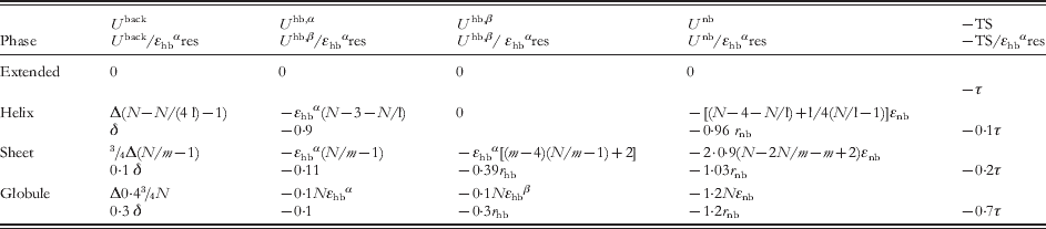
In Fig. 7a, the δ versus r nb projection is reported at τ=0 and r hb=1·1. This value is an average value for the relative strength of hydrogen bonds in sheets relative to those in helices, although both are known to depend on the amino acid type and on the level of salvation (Arora & Jayaram, Reference Arora and Jayaram1996) and are correlated to the sheet versus helix propensity (Bay & Englander, Reference Bay and Englander1994). The graph shows that for small values of r nb (~0·1), only well-defined secondary structures are stable, while the random coil can be stable for values of r nb~1. According to the analysis of section 4, such large values of r nb are adopted in the Sorenson–Head-Gordon model, while smaller values are more typical of (partially) biased models or of models in Alemani et al. (Reference Alemani, Collu, Cascella and Dal Peraro2010) and Tozzini et al. (Reference Tozzini, Rocchia and McCammon2006). Since intrinsically structured and unstructured amino acids exist, r nb (and all the other parameters) should assume the whole range of values, depending on the amino acid type. One possibility to correctly assign this dependency is to exploit some available secondary structure propensity scale, such as that by Chou and Fasman (CF) (Chou & Fasman, Reference Chou and Fasman1978), who give, for each amino acid, values of the helix, sheet and turn propensity (pα, pβ and pt). At fixed r hb thus the secondary structure propensity depends on δ and r nb. This can be expressed by simple relations δ=δ(pα, pβ) and r nb=r nb(pt, pα) such as those given in the caption of Fig. 7 (Tozzini, Reference Tozziniin preparation). Using them, and the CF propensity scale, the parameters δ and r nb for each amino acid are evaluated and the name of the amino acid placed on the (δ, r nb) plane accordingly. As can be seen, each amino acid is located in the correct region of the plane, according to its propensity, including those with hybrid sheet–helix propensity (located on the line separating the two phases) and the turn former amino acids.
This result was obtained assuming that the helix versus sheet propensity is mainly due to δ, while r nb modulates the tendency to form defined secondary structures versus random coils. However, one could also impute the helix versus sheet propensity to r hb and keep constant δ to an average value, since the strength of the hydrogen bonds is dependent on the hydration properties and on the amino acid type. In this case, a relationship r hb=r hb(pα, pβ) is needed to assign the r hb value to each amino acid (see the caption of Fig. 7), but the result is nearly the same and is reported in Fig. 7b: the amino acids are located correctly in the region of the planes according to their secondary structure propensity. A third way, the most physically plausible, is to vary both δ and r hb with the amino acid type, in a correlated way (correlation relation in the caption of Fig. 7) and the result is represented in Fig. 7c, giving the same accuracy as the two previous ones in locating the amino acids in the phase plane. Figure 7c reports the graph at room temperature (τ=0·03 if εhbα assumes the reasonable value of ~2 kcal/mol): with respect to the zero temperature the globule state is stabilized and the corresponding area enlarges at the expense of the structured areas.
Once these relationships between δ, r hb and r nb and pα, pβ and pt are fixed, one can study the phase diagram as a function of the temperature. This is reported in Fig. 7d–f for three different values of r hb corresponding to helix former, sheet former and ‘indifferent’ amino acids (areas enclosed in rectangles in Fig. 7c). The behaviors are quite different, and only in the case of the helix former the helix-to-sheet transition is observed, at a temperature modulated by r nb. In Fig. 7e, f, the temperature scale is expanded to show also the denaturation temperature (e.g. the transition to the extended state). These phase diagrams can help in fixing the parameterization based on the experimental knowledge of the transition temperatures. It is to be remarked that the evaluation of these phase diagrams is qualitative and should be checked by means of simulations of different peptide models spanning all the parameter space (work in progress; Tozzini, Reference Tozziniin preparation).
In conclusion, the suggested relationships r nb(pα, pt), r hb(pβ, pα) and δ(r hb) give simple operative prescriptions to evaluate the main energetic parameters for each amino acid, based on given amino acid secondary structure propensities. Although there is room for optimizing it, this recipe incorporates physical–chemical properties in the parameterization basically at null cost and possibly also some thermodynamic properties, through the secondary structure propensity. This does not exhaust the full parameterization: the relative weights of the angle and dihedral parameters in determining δ should be determined separately, possibly by means of FM or BI. The same is true for the relative energies of the two wells in U nb, which influences also more global properties such as the tertiary fold and the interactions between protein domains. These aspects must be systematically faced (and they are, by several authors: Korkuta & Hendrickson (Reference Korkuta and Hendrickson2009) and Trovato & Tozzini (Reference Trovato and Tozziniin preparation)) by FM- and/or BI-based methods.
Once optimized, this recipe for building the CG FF can in principle include the local structural accuracy (within the structural parameters via BI or FM procedures), the capability of predicting the relative secondary structure stabilities (included in the energetic parameters evaluated from the secondary structure propensities) and the tertiary–quaternary fold (via the accurate amino-acid-dependent parameterization of the U nb term).
6. Toward an optimal OB model: conclusions and perspectives
Although several models include one or more of the above-mentioned aspects, to my knowledge none include all of them that would be necessary for an optimal (predictive and accurate) model. UNRES, MARTINI and related models are probably those that better realize such an ideal, at the expense of additional beads and very complex functional forms. Remaining within the domain of the OB and truly minimalist models, the situation is summarized in Fig. 8 where the main classes of models cited in this paper are reported. The network models (green rectangle) are the simplest and bear the largest structural accuracy by definition due to the total bias toward a single reference structure that is the input of the problem. Their simplicity allows gaining the maximum efficiency; thus huge systems (up to viruses) can be studied. In the Go models, some unbiased terms start to be included, together with some elements of physics-based parameterization, which is a first step toward the transferability. These steps are more pronounced in the partially biased models, with a small amount of local bias left, which allows us to accurately represent the hydrogen bonds and other local strong interactions. These models bear a good structural accuracy and good predictive power, being suitable for general dynamics. The completely unbiased physics-based models such as that of Sorenson–Head-Gordon make the final step toward the transferability, dropping any bias toward single structures. However, in the present form, they bear low structural accuracy. This can be improved by enhancing the flexibility of the functional forms used in the FF terms and the accuracy of the parameterization. In the previous section, a general procedure to do that is proposed that involves combining FM- and/or BI-based methods with physics- and chemistry-based methods, which should ideally guide the parameterization of a model placed in the top right corner of the graph. Encouraging preliminary steps have been already performed for generic polypeptide models (Alemani et al. Reference Alemani, Collu, Cascella and Dal Peraro2010; Tozzini et al. Reference Tozzini, Rocchia and McCammon2006).
Upper part: schematic summary of the characteristics of the main classes of OB CG models. The models are placed in the diagram approximately according to their structural accuracy and predictive power. The pictures indicate very roughly the size of the system treated and the functions of the model. At the bottom a schematic representation of the release of the bias is shown, which parallels the increase in transferability. In blue, the polypeptide backbone is schematically represented. The red lines connecting the Cα represent the biased interactions. Dashed lines represent interactions with hybrid biased–unbiased character (sometimes occurring in Go models).

In general, however, although the goal is clear and the routes to reach it start now to be less confused, the minimalist models are, in my opinion, still far from a possible standard such as that reached, for instance, for AA FF. In spite of this, I believe that efforts to systematically study and parameterize a minimalist model for proteins (and more in general for bio-molecules) should not be abandoned, because minimalist models are those that combine a sufficient level of resolution with the largest possible gain in computational cost; thus they are the key to address bio-systems on biologically interesting size and time scales.
7. Acknowledgements
I thank Fabio Trovato and Armida Di Fenza for useful discussions.