1 Introduction
Flow in a differentially heated rotating annulus has attracted the attention of scientists from several different fields over the past decades due to its relevance to geophysical phenomena (Read et al.
Reference Read, Pérez, Moroz, Young, von Larcher and Williams2014) and buoyancy-induced flows in engineering applications (Owen & Long Reference Owen and Long2015). This simple configuration provides a multitude of complex dynamics when control parameters such as the rotation rate
 $\unicode[STIX]{x1D6FA}$
, the temperature difference
 $\unicode[STIX]{x0394}T$
and the Prandtl number are varied, and therefore is also employed to study aspects of fundamental fluid dynamics, such as bifurcations, onset of instabilities and transition to turbulence.
In early experimental studies of flow in a vertical rotating annulus subject to a horizontal temperature gradient (see Hide & Mason (Reference Hide and Mason1975) for a review), four basic flow regimes have been identified. Hide (Reference Hide1958) performed experiments using water and observed that for sufficiently small values of the rotation rate
 $\unicode[STIX]{x1D6FA}$
, the flow is axisymmetric and confined to a meridional circulation induced by gravitational buoyancy. A second regime occurs when the rotation rate is increased above a critical value, where Coriolis forces tend to suppress the meridional motion and induce an azimuthal pressure gradient, creating baroclinic waves that propagate along the azimuthal direction of the annulus. In this regime the baroclinic waves can be either steady or vacillating, i.e. their shape and size can change over time. Above a certain value of the rotational speed the flow becomes irregular and no coherent shape or size of the baroclinic waves is discernible. This regime is also known as geostrophic turbulence. Finally, the fourth regime is also axisymmetric and occurs when the temperature difference is so small that the Coriolis force does not trigger the baroclinic instability, regardless of the rotation rate. These flow regimes encountered in the baroclinic annulus are usually represented in a regime diagram in terms of a thermal Rossby number
 $\unicode[STIX]{x1D6E9}$
and a Taylor number
 $Ta$
, given by
 $$\begin{eqnarray}\displaystyle & \displaystyle \unicode[STIX]{x1D6E9}=\frac{g\unicode[STIX]{x1D6FC}\unicode[STIX]{x0394}Td}{\unicode[STIX]{x1D6FA}^{2}(b-a)^{2}}, & \displaystyle\end{eqnarray}$$
 $$\begin{eqnarray}\displaystyle & \displaystyle Ta=\frac{4\unicode[STIX]{x1D6FA}^{2}(b-a)^{5}}{\unicode[STIX]{x1D708}^{2}d}, & \displaystyle\end{eqnarray}$$
where
 $g$
is the acceleration of gravity,
 $\unicode[STIX]{x1D6FC}$
and
 $\unicode[STIX]{x1D708}$
are the thermal expansion coefficient and kinematic viscosity of the fluid, respectively,
 $\unicode[STIX]{x0394}T$
is the temperature difference between the cylindrical walls,
 $d$
is the height of the annulus and
 $a$
and
 $b$
are the inner and outer radii. Note that the thermal Rossby number provides a measure of the ratio of inertial over Coriolis effects, while the Taylor number is interpreted as the ratio of Coriolis over viscous effects.
After the four flow regimes were identified experimentally, more detailed analyses were carried out both experimentally (Castrejón-Pita & Read Reference Castrejón-Pita and Read2007; Vincze Reference Vincze, Borchert, Achatz, von Larcher, Baumann, Hertel, Remmler, Beck, Alexandrov and Egbers2015) and numerically using direct numerical simulation (DNS) (Randriamampianina et al. Reference Randriamampianina, Früh, Read and Maubert2006; Read et al. Reference Read, Maubert, Randriamampianina and Früh2008; Vincze Reference Vincze, Borchert, Achatz, von Larcher, Baumann, Hertel, Remmler, Beck, Alexandrov and Egbers2015) and linear stability analysis (Lewis & Nagata Reference Lewis and Nagata2004). The amplitude vacillation regime has attracted much attention, as in this regime chaotic behaviour starts to set in and phenomena such as hysteresis and wave interactions arise. Also, the study of this regime is crucial to understand the transition towards geostrophic turbulence. For a recent overview of amplitude vacillation and baroclinic flows in general, the reader is referred to Früh (Reference Früh, von Larcher and Williams2014) and Read et al. (Reference Read, Pérez, Moroz, Young, von Larcher and Williams2014), respectively.
Although the baroclinic instability is induced by the action of Coriolis forces, this type of instability is characterised by having a centrifugal acceleration which is smaller than gravity. When the ratio of the centrifugal acceleration to gravity, given by a Froude number defined as
 $Fr=\unicode[STIX]{x1D6FA}^{2}r/g$
, is larger than unity, the instability mechanism that induces convection is fundamentally different from that of the baroclinic instability. Rather than being induced by the Coriolis force, the instability occurs due to the action of the centrifugal force combined with a negative density gradient in the radial direction. Such instability is analogous to that observed in a fluid layer heated from below under gravity (Rayleigh–Bénard convection). Read et al. (Reference Read, Maubert, Randriamampianina and Früh2008) have shown that as the Froude number is increased above unity in a baroclinic annulus, the convection rolls tend to be less tilted than in the cases where the baroclinic instability is present, i.e. at lower
 $Fr$
. Such convection rolls showing little dependence on the axial coordinate are also referred to as Taylor columns and have been observed experimentally by Busse & Carrigan (Reference Busse and Carrigan1974), who used an apparatus in which the gap between the two cylinders was very small and where the centrifugal acceleration was up to seven times
 $g$
. In studies where the centrifugal acceleration is assumed much higher than gravity, the onset of convection and the transition between different regimes is analysed in terms of a centrifugal Rayleigh number, which measures the ratio of centrifugal buoyancy over viscous dissipation, defined as
 $$\begin{eqnarray}\displaystyle Ra=\frac{\unicode[STIX]{x1D6FA}^{2}r_{0}\unicode[STIX]{x1D6FC}\unicode[STIX]{x0394}T(b-a)^{3}}{\unicode[STIX]{x1D708}\unicode[STIX]{x1D705}}\equiv \frac{\unicode[STIX]{x1D6E9}FrTaPr}{4}\equiv \frac{TaPr\unicode[STIX]{x1D6FC}\unicode[STIX]{x0394}TAR_{c}}{8}, & & \displaystyle\end{eqnarray}$$
where
 $r_{0}$
is the mean radius,
 $\unicode[STIX]{x1D705}$
is the thermal diffusivity,
 $A=d/(b-a)$
is the aspect ratio,
 $R_{c}=(b+a)/(b-a)$
is the curvature parameter and the Froude number
 $Fr$
is evaluated at
 $r=r_{0}$
. In numerical studies it is also common to consider that the system is subject to a radial gravitational acceleration
 $g_{r}$
, in which case
 $\unicode[STIX]{x1D6FA}^{2}r_{0}$
is replaced by
 $g_{r}$
in the definition of
 $Ra$
. For these cases the Taylor and Rayleigh numbers are not coupled by the rotational speed
 $\unicode[STIX]{x1D6FA}$
. The onset of convection for such configuration has been studied using linear stability analysis, see e.g. Zhang & Greed (Reference Zhang and Greed1998) and references therein. Here, we are concerned with configurations in which buoyancy is induced by the action of the centrifugal acceleration, which differs from the case with radial gravity since the acceleration varies with
 $r$
, thus affecting the dynamics, especially when the radial gap is not small. In the nonlinear regime, analogously to the case of baroclinic waves, Taylor columns also have a well-defined shape and size that does not change over time in certain regions of the parameter space, but when a critical Rayleigh number is reached, asymmetric and vacillating flow occur (see Or & Busse Reference Or and Busse1987; Schnaubelt & Busse Reference Schnaubelt and Busse1992).
Whilst the studies described in the previous paragraphs were motivated by applications involving atmospheric flows and convection in the fluid core of planets, the problem of buoyancy-induced flow in a rotating annulus is also of interest for the engineering community. Specifically, such flows occur in rotor/rotor cavities of internal air systems used to provide cooling for certain components of gas turbines. The outer cylindrical part of these cavities (shroud) is usually hotter than the inner part, where cooling air flows axially, which creates a strong buoyancy-generated flow induced by the centrifugal force. These flows are recognised to be very challenging to model (Chew & Hills Reference Chew and Hills2007) and have been studied both experimentally (Bohn et al. Reference Bohn, Deuker, Emunds and Gorzelitz1995) and numerically (Sun et al. Reference Sun, Kifoil, Chew and Hills2004; King, Wilson & Owen Reference King, Wilson and Owen2007; Pitz et al. Reference Pitz, Chew, Marxen and Hills2017). In these studies the main focus was on obtaining predictions for the heat transfer rates on the cylindrical walls, and also on understanding the general structure of the flow. The unsteady nature of these flows has an impact on the temperature distribution on the cavity disks, which must be known in order to improve the prediction of radial growth during an engine flight cycle. The use of model-free approaches has potential to provide an accurate description of the unsteady events happening in buoyancy-induced flows in rotating cavities and a better understanding of how those events affect the temperature and heat transfer distributions. Studying the onset of convection and the transition mechanisms gives insight into the physics of these flows.
In this work we investigate the onset of convection from the conduction state and the transition from the intermediate state in which Taylor columns appear to fully chaotic flow, where convection rolls are less evident. Linear stability analysis is employed to obtain critical values of the Rayleigh number for the onset of convection for different radius ratios and also to find the most unstable azimuthal wavenumbers. Using DNS, we analyse how the shape of infinitesimal disturbances influences the formation of convection rolls, and how those rolls break up as the turbulent state is reached. Our geometry and boundary conditions are chosen to provide a simplified representation of a compressor rotating cavity, consisting of a sealed rotating annulus bounded by two parallel, insulated disks, and by cold and hot inner and outer cylindrical walls, respectively. As we focus on cases where the centrifugal acceleration is the leading-order force driving the instability, gravitational effects are neglected.
The paper is organised as follows. In § 2 the geometry, boundary conditions and range of parameters investigated are presented, as well as the numerical methods employed to solve the governing equations. Section 3 presents results obtained from linear stability analysis and in § 4 we discuss the transition to the nonlinear regime.
2 Problem description and numerical method
2.1 Geometry and governing equations
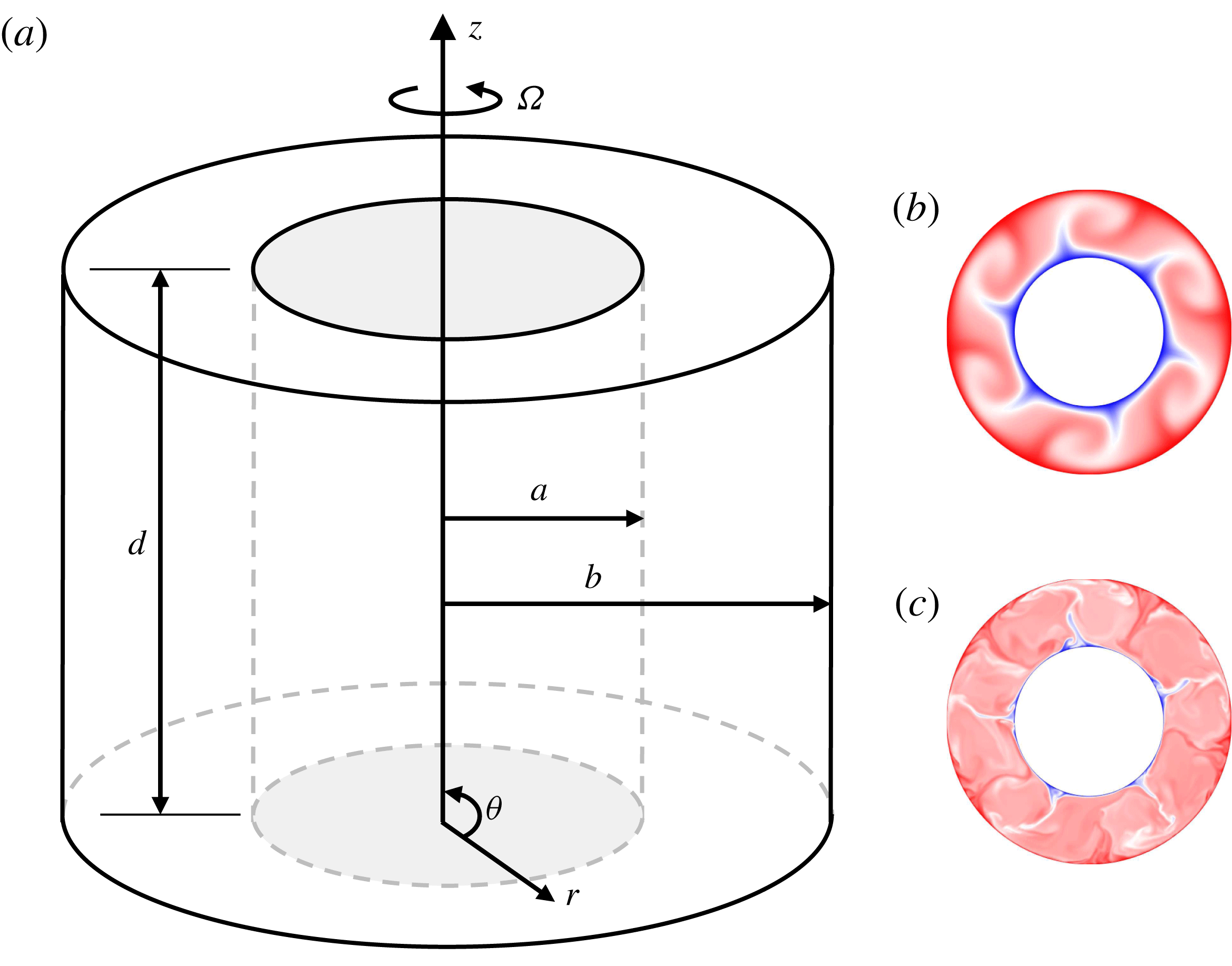
Consider an incompressible fluid bounded by a cylindrical annulus with flat end walls, rotating about its axis at a constant angular speed
 $\unicode[STIX]{x1D6FA}$
, cf. figure 1(a). The centrifugal force induced by rotation is assumed to be the leading-order body force, therefore the effect of gravity is neglected, i.e. we assume that
 $Fr\gg 1$
. The inner and outer cylindrical walls are kept at constant temperatures,
 $T_{a}$
and
 $T_{b}$
, respectively, where
 $T_{b}>T_{a}$
, whilst the two disks are adiabatic. Since the whole system rotates at the same angular speed, the flow is generated purely by buoyancy effects. The physical dimensions of the cavity are chosen to match the experimental set-up employed by Bohn et al. (Reference Bohn, Deuker, Emunds and Gorzelitz1995), who used
 $a=0.125~\text{m}$
,
 $b=0.24~\text{m}$
,
 $d=0.12~\text{m}$
and air as the working fluid, giving
 $Pr\equiv \unicode[STIX]{x1D708}/\unicode[STIX]{x1D705}=0.7$
, where
 $Pr$
is the Prandtl number. With these dimensions, the aspect ratio, radius ratio and curvature parameter are
 $A=1.04$
,
 $\unicode[STIX]{x1D702}=a/b=0.52$
and
 $R_{c}=3.2$
. Although the limited data obtained from the experiments do not allow for a comparison against our results, the choice of this set-up was motivated by its relevance as a typical industrial configuration. The dimensions were kept fixed in the DNSs, but for the linear analysis of the onset of convection we have varied the radius ratio
 $\unicode[STIX]{x1D702}$
within the interval
 $0.2\leqslant \unicode[STIX]{x1D702}\leqslant 0.99$
. While the analysis is focused on the case with no-slip end walls, for some cases we include results obtained using periodicity along the axial direction.
In order to be consistent with the nomenclature adopted in the turbomachinery community, the non-dimensional numbers used here are the Rayleigh and Reynolds numbers, the latter given by
 $$\begin{eqnarray}\displaystyle Re=\frac{\unicode[STIX]{x1D6FA}r_{0}(b-a)}{\unicode[STIX]{x1D708}}, & & \displaystyle\end{eqnarray}$$
where
 $r_{0}=(b+a)/2$
and the kinematic viscosity has a constant value in all cases,
 $\unicode[STIX]{x1D708}=1.5\times 10^{-5}~\text{m}^{2}~\text{s}^{-1}$
. With this definition, the Rayleigh and Reynolds numbers are related by,
 $$\begin{eqnarray}\displaystyle Ra=\frac{2Re^{2}Pr\unicode[STIX]{x1D6FC}\unicode[STIX]{x0394}T}{R_{c}}. & & \displaystyle\end{eqnarray}$$
Here we restrict our attention to the cases where the temperature difference is constant, so
 $\unicode[STIX]{x1D6FC}\unicode[STIX]{x0394}T$
is kept at a fixed value,
 $\unicode[STIX]{x1D6FC}\unicode[STIX]{x0394}T=0.1$
. The Reynolds and Rayleigh numbers then change simultaneously when the angular speed
 $\unicode[STIX]{x1D6FA}$
is varied, and for this reason our results are presented in terms of the Rayleigh number only. For reference, the two cases analysed in more detail are
 $Ra=10^{5}$
, giving
 $Re=1.5\times 10^{3}$
and
 $Ta=3.5\times 10^{6}$
, and
 $Ra=10^{8}$
, giving
 $Re=4.8\times 10^{4}$
and
 $Ta=3.5\times 10^{9}$
. Figure 1(b,c) shows examples of instantaneous temperature contours obtained in the nonlinear regime for
 $Ra=10^{5}$
and
 $Ra=10^{8}$
, respectively, at the mid-axial plane. As discussed in more detail later, for
 $Ra=10^{5}$
the flow is dominated by an initially perturbed azimuthal mode and its harmonics, while for
 $Ra=10^{8}$
many modes contribute significantly to the total energy.
(a) Geometry of a rotating annulus with end walls. The entire system rotates at a constant angular speed
 $\unicode[STIX]{x1D6FA}$
, the temperatures of the cylindrical surfaces are such that
 $T_{b}>T_{a}$
and the two disks are adiabatic. Instantaneous temperature contours at the mid-axial position in the nonlinear regime for (b)
 $Ra=10^{5}$
and (c)
 $Ra=10^{8}$
, ranging from
 $T_{a}$
to
 $T_{b}$
.

For the DNS calculations, we solve the Navier–Stokes–Boussinesq equations, where the mass, momentum and energy conservation equations are, in non-dimensional form,
 $$\begin{eqnarray}\displaystyle & \displaystyle \unicode[STIX]{x1D735}\boldsymbol{\cdot }\boldsymbol{u}^{\ast }=0, & \displaystyle\end{eqnarray}$$
 $$\begin{eqnarray}\displaystyle & \displaystyle \frac{\unicode[STIX]{x2202}\boldsymbol{u}^{\ast }}{\unicode[STIX]{x2202}t}+\boldsymbol{u}^{\ast }\boldsymbol{\cdot }\unicode[STIX]{x1D735}\boldsymbol{u}^{\ast }=-\unicode[STIX]{x1D735}p^{\ast }+Pr\unicode[STIX]{x1D6FB}^{2}\boldsymbol{u}^{\ast }-\frac{4PrRe}{R_{c}}\boldsymbol{z}\times \boldsymbol{u}^{\ast }+\boldsymbol{F}, & \displaystyle\end{eqnarray}$$
 $$\begin{eqnarray}\displaystyle & \displaystyle \frac{\unicode[STIX]{x2202}T^{\ast }}{\unicode[STIX]{x2202}t}+\boldsymbol{u}^{\ast }\boldsymbol{\cdot }\unicode[STIX]{x1D735}T^{\ast }=\unicode[STIX]{x1D6FB}^{2}T^{\ast }, & \displaystyle\end{eqnarray}$$
where the reduced pressure is, in dimensional form, given by
 $p=p^{\star }-(|\unicode[STIX]{x1D734}\times \boldsymbol{r}|^{2})/2$
,
 $p^{\star }$
being the total pressure and
 $\boldsymbol{z}$
is the unit vector in the axial direction. The equations above are non-dimensionalised using
 $(b-a)$
as a length scale,
 $\unicode[STIX]{x1D705}/(b-a)$
as a velocity scale,
 $(b-a)^{2}/\unicode[STIX]{x1D705}$
as a time scale and
 $\unicode[STIX]{x0394}T$
as a temperature scale. The forcing term
 $\boldsymbol{F}$
represents buoyancy induced by the centrifugal acceleration,
 $$\begin{eqnarray}\displaystyle \boldsymbol{F}=-\frac{2PrRa}{R_{c}}\left(r^{\ast }+\frac{\unicode[STIX]{x1D702}}{1-\unicode[STIX]{x1D702}}\right)T^{\ast }\boldsymbol{r}, & & \displaystyle\end{eqnarray}$$
where
 $r^{\ast }=(r-a)/(b-a)$
. Note that the equations are solved in a rotating reference frame and that density variations are accounted for only when multiplied by the centrifugal force and are calculated as a linear function of the temperature variation,
 $\unicode[STIX]{x1D70C}=\unicode[STIX]{x1D70C}_{0}[1-\unicode[STIX]{x1D6FC}(T-T_{a})]$
. The non-dimensional temperature and axial coordinate are defined as
 $T^{\ast }=(T-T_{a})/\unicode[STIX]{x0394}T$
and
 $z^{\ast }=z/d$
. With these definitions, the boundary conditions are, in non-dimensional form,
 $$\begin{eqnarray}\boldsymbol{u}^{\ast }(0,\unicode[STIX]{x1D703},z^{\ast })=\boldsymbol{u}^{\ast }(1,\unicode[STIX]{x1D703},z^{\ast })=\boldsymbol{u}^{\ast }(r^{\ast },\unicode[STIX]{x1D703},0)=\boldsymbol{u}^{\ast }(r^{\ast },\unicode[STIX]{x1D703},1)=0,\end{eqnarray}$$
 $$\begin{eqnarray}\displaystyle & \displaystyle T^{\ast }(0,\unicode[STIX]{x1D703},z^{\ast })=0, & \displaystyle\end{eqnarray}$$
 $$\begin{eqnarray}\displaystyle & \displaystyle T^{\ast }(1,\unicode[STIX]{x1D703},z^{\ast })=1, & \displaystyle\end{eqnarray}$$
 $$\begin{eqnarray}\displaystyle & \displaystyle \unicode[STIX]{x2202}_{z}T^{\ast }(r^{\ast },\unicode[STIX]{x1D703},0)=\unicode[STIX]{x2202}_{z}T^{\ast }(r^{\ast },\unicode[STIX]{x1D703},1)=0. & \displaystyle\end{eqnarray}$$
For the linear stability analysis, the perturbation equations (not shown here for brevity) are solved for a given base flow and the perturbed variables
 $\boldsymbol{u}^{\prime }$
and
 $T^{\prime }$
are set to zero on all boundaries.
2.2 Numerical methods
The governing equations are solved using a spectral element–Fourier technique formulated in cylindrical coordinates, described by Blackburn & Sherwin (Reference Blackburn and Sherwin2004). Quadrilateral expansion bases are constructed in two dimensions using Lagrange polynomials interpolated at the zeros of Gauss–Lobatto–Legendre polynomials, and are used to discretise the governing equations in the radial and axial directions. For the azimuthal direction, Fourier expansions are used to take advantage of the geometry homogeneity along this coordinate. The equations are integrated in time using the second-order, semi-implicit, stiffly stable scheme described by Karniadakis, Israeli & Orszag (Reference Karniadakis, Israeli and Orszag1991). A base version of the code has been modified to account for buoyancy due to the centrifugal force induced by rotation. To verify this implementation, we have reproduced the baroclinic waves reported by Read et al. (Reference Read, Maubert, Randriamampianina and Früh2008) at different Taylor and Froude numbers. Specifically, we observed that as the local Froude number is increased above unity, the flow structure ceases to be dominated by axial gravity and centrifugal buoyancy effects become stronger.
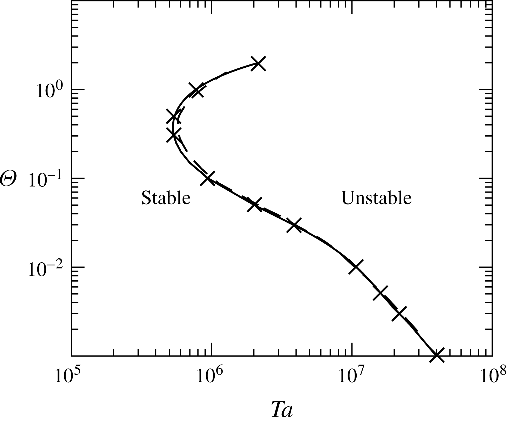
To compute growth rates and mode shapes for different azimuthal wavenumbers, we use an eigenvalue solver, which is implemented using a time-stepper method. Given a steady, two-dimensional base flow (as is the case here), the linearised form of the Navier–Stokes equations are integrated for a given time period. An iterative solution to the eigensystem is then obtained using an orthogonal projection of the linear operator onto a Krylov subspace. For the problem investigated here, specifically, the base flow is two-dimensional with three velocity components, whilst the modes obtained are three-dimensional, again using Fourier expansions to treat the periodic direction. For further details on the method and implementation of the linear stability analysis code, please refer to Tuckerman & Barkley (Reference Tuckerman and Barkley2000) and Barkley, Blackburn & Sherwin (Reference Barkley, Blackburn and Sherwin2008). The original implementation does not consider the energy equation for incompressible flow, which we have implemented, along with the corresponding buoyancy terms in the momentum equations. To verify this new implementation, the critical curves for the onset of instabilities in a rotating annulus with axial gravity and centrifugal buoyancy reported by Lewis & Nagata (Reference Lewis and Nagata2004) have been reproduced, as shown in figure 2. The curve represents the critical values of the Rossby and Taylor numbers for the onset of three-dimensional instability. As shown, the results are in excellent agreement with those reported by Lewis & Nagata (Reference Lewis and Nagata2004).
Comparison of current results (solid line and marker) with the numerical results reported by Lewis & Nagata (Reference Lewis and Nagata2004) (dashed line) for the onset of three-dimensional instabilities in a rotating annulus.

2.3 Details of the computations
For the linear stability analysis, a mesh with 50 spectral elements was employed. The polynomial order
 $P$
of the two-dimensional expansion basis was chosen based on two convergence studies using cases representative of the calculations performed in this work. In the first case the smallest Rayleigh number
 $Ra_{c}$
giving an unstable solution was calculated, as well as the critical azimuthal wavenumber
 $k_{c}$
, for different values of
 $P$
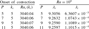
. As illustrated on the left-hand side of table 1, the results are very similar for all values of
 $P$
. Note that, since the domain is cylindrical, only integer values of
 $k_{c}$
are considered. The second convergence study was carried out perturbing the base flow at the highest value of the Rayleigh number considered in this work,
 $Ra=10^{8}$
, and evaluating the growth rate
 $\unicode[STIX]{x1D706}_{r}$
and the angular frequency
 $\unicode[STIX]{x1D706}_{i}$
of the leading, most unstable eigenvalue. The values obtained from this analysis for different
 $P$
are shown on the right-hand side of table 1, where no significant differences are observed for
 $P\geqslant 7$
. Based on this study, we adopted
 $P=7$
to carry out all the linear stability analyses reported in this paper.
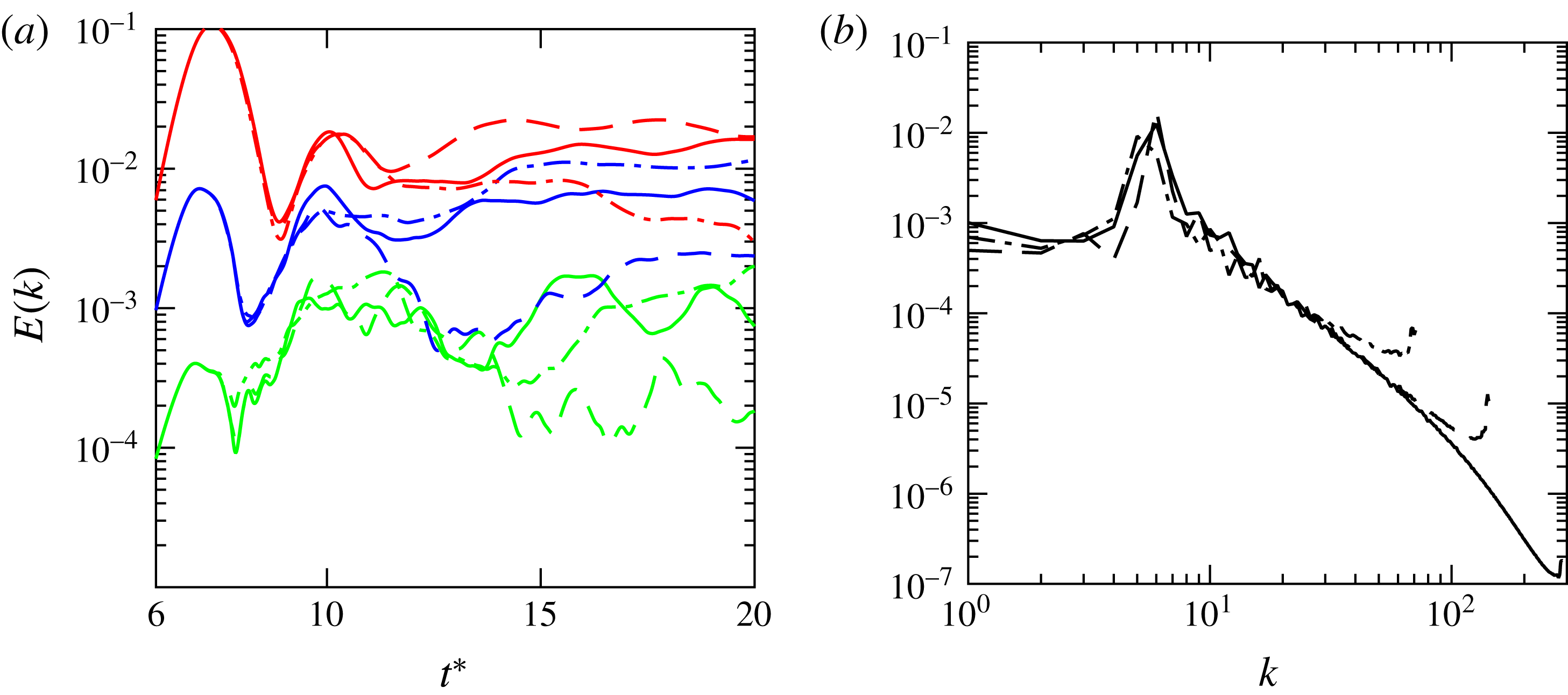
(a) Effect of
 $N_{\unicode[STIX]{x1D703}}$
on the evolution of modal energies over time for modes 4 (bottom) to 6 (top) at
 $Ra=10^{8}$
after saturation. (b) Modal energy as a function of the mode number
 $k$
, time averaged in the interval
 $10\leqslant t^{\ast }\leqslant 20$
. — ⋅ —
 $N_{\unicode[STIX]{x1D703}}=144$
; – –
 $N_{\unicode[STIX]{x1D703}}=288$
; ——
 $N_{\unicode[STIX]{x1D703}}=576$
.

Effect of the polynomial order on quantities obtained from linear stability analysis. The mesh used has 50 quadrilateral spectral elements.

The nonlinear analyses are performed using a mesh with 252 quadrilateral spectral elements in the
 $r$
–
 $z$
plane. To perturb the motionless basic state, a series of sinusoidal waves with an amplitude of 0.001 % of the mean temperature is added to the temperature field. Using this approach, one can follow the evolution of disturbances of a given wavenumber
 $k$
, and analyse how they grow in time and how they behave during and after the transition. In figure 3(a) the temporal evolution of the modal kinetic energy,
 $E(k)$
, of disturbances with azimuthal wavenumbers ranging from 4 to 6 is presented for a mesh with
 $P=9$
and
 $N_{\unicode[STIX]{x1D703}}=144$
, 288 and 576, for
 $Ra=10^{8}$
(note that the energy corresponding to
 $k=0$
, i.e. energy of the mean flow, is not shown). As the curves obtained with the three meshes collapse during the initial stage, the figure only shows the behaviour of
 $E(k)$
after the saturation takes place. The non-dimensional time used is given by
 $t^{\ast }=\unicode[STIX]{x1D6FA}t/2\unicode[STIX]{x03C0}$
, so it corresponds to the number of revolutions of the system. For
 $N_{\unicode[STIX]{x1D703}}=144$
, the energy of mode 6 starts to decay and is overtaken by mode 5 at
 $t^{\ast }\approx 14$
, when the flow becomes turbulent. For the other two values of
 $N_{\unicode[STIX]{x1D703}}$
, the behaviour of the modes is qualitatively similar, with mode 6 remaining as the most energetic. A plot of the modal kinetic energy versus the azimuthal wavenumber is presented in figure 3(b) for the three meshes, again excluding the mean flow energy. The energy for each mode was obtained by time averaging the modal energies in the interval
 $10\leqslant t^{\ast }\leqslant 20$
, where the flow is turbulent. The range of resolved scales increases significantly when
 $N_{\unicode[STIX]{x1D703}}$
is increased. Note that in all cases there is a small increase of the energy at high
 $k$
, which is due to aliasing effects. Despite this, the behaviour of the low
 $k$
modes is not affected by the resolution when
 $N_{\unicode[STIX]{x1D703}}$
is increased from 288 to 576, cf. figure 3(a). For the purposes of this work, we decided to use
 $N_{\unicode[STIX]{x1D703}}=288$
in the calculations, as the behaviour of the disturbances is similar to that observed for
 $N_{\unicode[STIX]{x1D703}}=576$
, and also because figure 3(b) shows that a sufficiently broad range of scales is resolved. Repeating the calculations using
 $P=7$
no differences were observed, so
 $P=7$
was adopted for the nonlinear calculations.
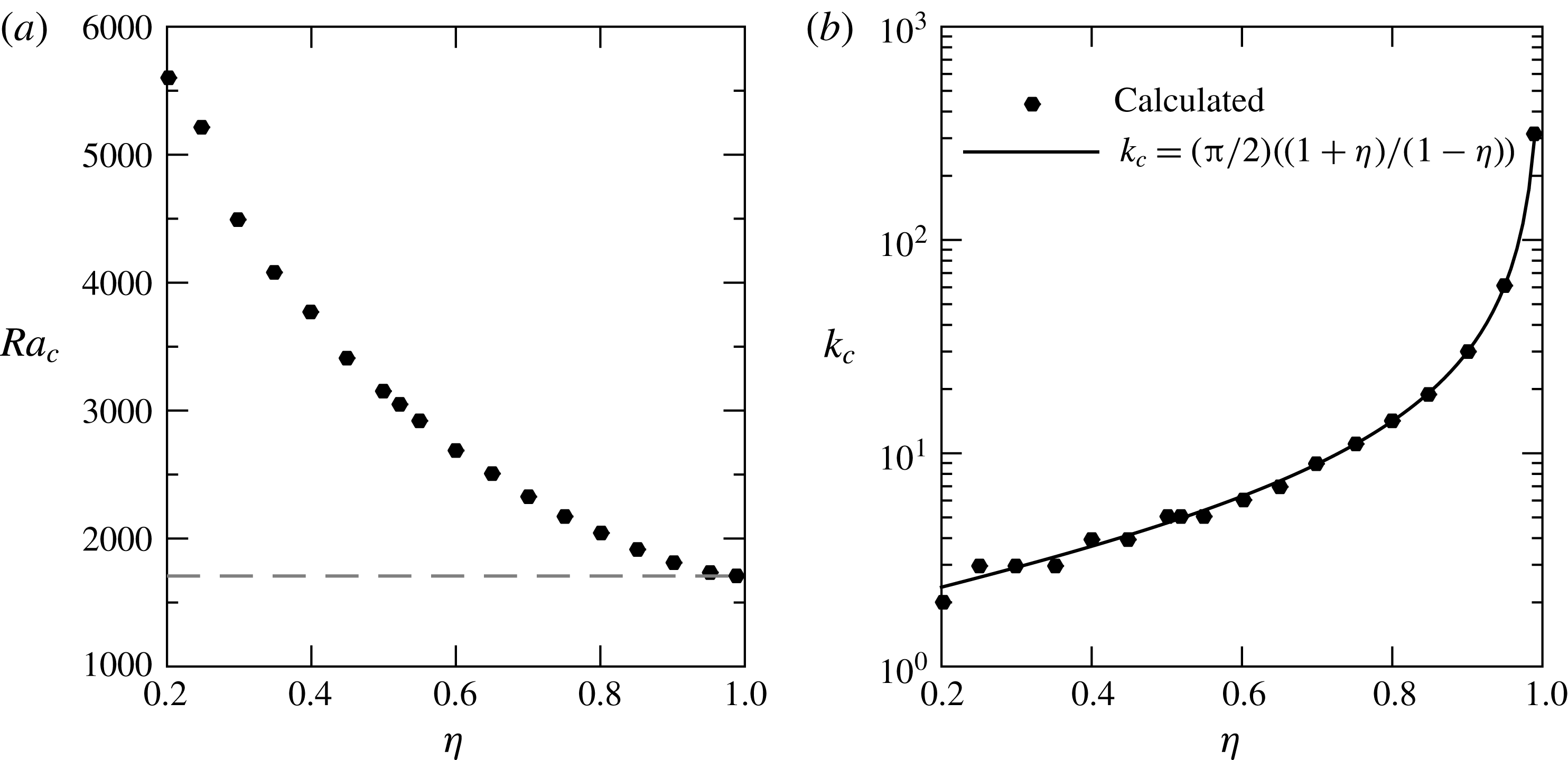
(a) Critical Rayleigh number
 $Ra_{c}$
for the onset of convection as a function of the radius ratio
 $\unicode[STIX]{x1D702}$
. The dashed line corresponds to the critical Rayleigh number for flow between parallel plates heated from below. The extra point at
 $\unicode[STIX]{x1D702}=0.52$
corresponds to the geometry considered in more detail throughout the paper. (b) Critical azimuthal wavenumber
 $k_{c}$
versus
 $\unicode[STIX]{x1D702}$
.

3 Linear stability analysis
3.1 Onset of convection
To analyse the onset of convection we consider a base flow consisting of solid-body rotation for the velocity components and a pure conduction temperature profile,
 $$\begin{eqnarray}\displaystyle & \displaystyle \boldsymbol{u}^{\ast }=\mathbf{0}, & \displaystyle\end{eqnarray}$$
 $$\begin{eqnarray}\displaystyle & \displaystyle T^{\ast }(r^{\ast })=\frac{\log (1+(b-a)r^{\ast }/a)}{\log (b/a)}. & \displaystyle\end{eqnarray}$$
This base state is perturbed for different integer azimuthal wavenumbers
 $k$
, and we look for the critical values of the Rayleigh number,
 $Ra_{c}$
, that give a zero growth rate to the leading eigenvalues. This procedure of finding
 $Ra_{c}$
was repeated for 18 values of the radius ratio
 $\unicode[STIX]{x1D702}$
within the interval
 $0.2\leqslant \unicode[STIX]{x1D702}\leqslant 0.99$
, keeping the axial length constant.
As the radius ratio
 $\unicode[STIX]{x1D702}$
is increased, the critical Rayleigh number for the onset of convection decreases, and the critical azimuthal wavenumber increases, as shown in figure 4. As expected, in the asymptotic limit
 $\unicode[STIX]{x1D702}\rightarrow 1$
, the value of
 $Ra_{c}$
approaches that corresponding to natural convection under gravity heated from below, for which
 $Ra_{c}\approx 1708$
, as indicated by a dashed line in figure 4(a). The calculations also reveal that the conductive state loses its stability to modes formed of pairs of convection cells whose azimuthal length are very close to the gap dimension. Assuming that, at the onset of convection, the length of a cell at
 $r=r_{0}$
is exactly equivalent to the gap width, the critical wavenumber is given by
 $$\begin{eqnarray}\displaystyle k_{c}=\frac{\unicode[STIX]{x03C0}r_{0}}{b-a}=\frac{\unicode[STIX]{x03C0}}{2}\frac{1+\unicode[STIX]{x1D702}}{1-\unicode[STIX]{x1D702}}. & & \displaystyle\end{eqnarray}$$
This expression was employed by Owen (Reference Owen2010) to estimate the number of pairs of cells in a rotating cavity in the nonlinear regime. Figure 4(b) shows that (3.2) is an excellent approximation to the critical wavenumber, even for relatively small values of
 $\unicode[STIX]{x1D702}$
. Note that (3.2) returns non-integer values, and that is the reason why it is slightly off the calculated values of
 $k_{c}$
for low
 $\unicode[STIX]{x1D702}$
. The fact that Owen (Reference Owen2010) has suggested that (3.2) is a suitable approximation in the nonlinear regime suggests that the basic structure that arises on the onset of convection persists even in the turbulent state, albeit in a less pronounced manner.
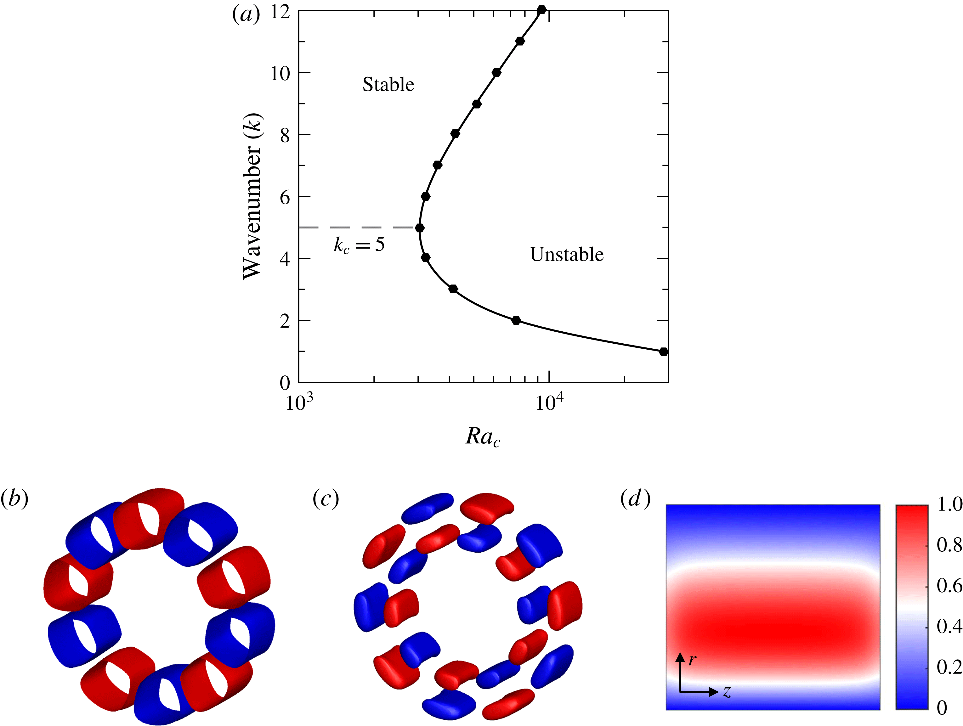
(a) Critical Rayleigh number
 $Ra_{c}$
for the onset of convection for various azimuthal wavenumbers
 $k$
; mode shapes of temperature (b) and azimuthal velocity (c) for
 $k=5$
showing positive (red) and negative (blue) perturbations; (d) amplitude of temperature perturbation in Fourier space in a
 $r$
–
 $z$
plane for
 $k=5$
normalised by the maximum value.
 $\unicode[STIX]{x1D702}=0.52$
for all plots.

We now focus on the case with
 $a=0.125~\text{m}$
and
 $b=0.24~\text{m}$
, or
 $\unicode[STIX]{x1D702}=0.52$
, as employed in the experiment by Bohn et al. (Reference Bohn, Deuker, Emunds and Gorzelitz1995). Figure 5(a) shows the critical Rayleigh numbers obtained for 12 azimuthal wavenumbers. From this figure, it can be seen that the lowest value of
 $Ra_{c}$
for the onset of convection corresponds to a critical wavenumber
 $k_{c}=5$
. The shape of the eigenmode obtained setting
 $k=5$
is illustrated in figure 5(b,c), for the temperature and azimuthal velocity component, respectively. These indicate that the flow structure at the onset of convection consists of pairs of counter rotating cells, akin to convection under a gravitational field. Although the mode shapes seem to be invariant along the axial direction, a plot of the amplitude of the temperature perturbation in Fourier space in two dimensions reveals that the modes are tilted near the end walls of the cavity, as shown in figure 5(d). This tilt is caused by the presence of the disks with no-slip boundary conditions, which forces the flow to be three-dimensional. For higher Rayleigh numbers, the effect of the disks becomes less significant and confined to thin boundary layers.
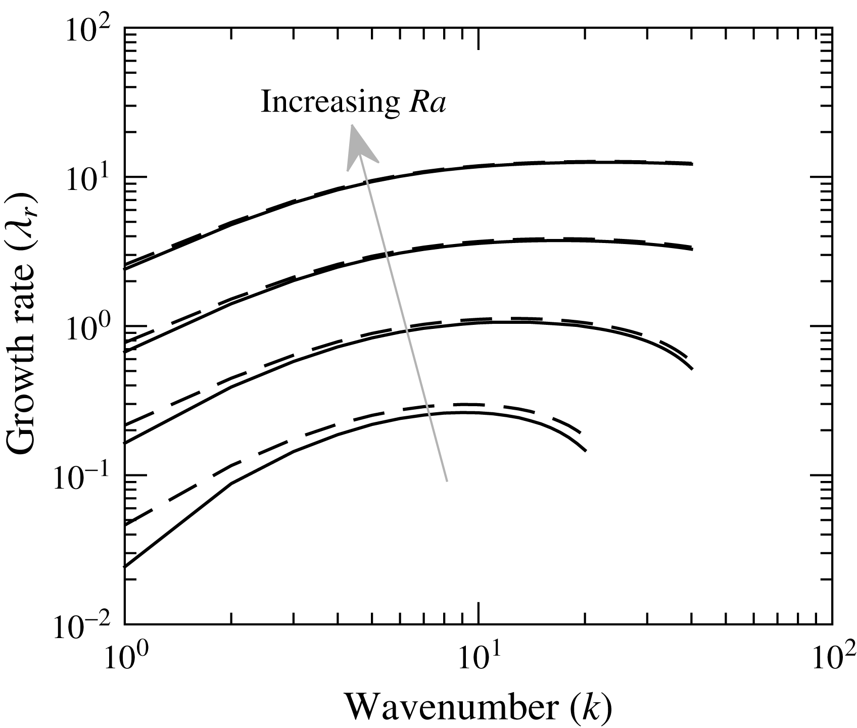
Growth rate
 $\unicode[STIX]{x1D706}_{r}$
as a function of the azimuthal wavenumber
 $k$
for
 $Ra=10^{5}$
,
 $Ra=10^{6}$
,
 $10^{7}$
and
 $10^{8}$
. The dashed lines indicate solutions obtained without end walls, i.e. considering periodicity along the axial direction.

3.2 Linear growth of unstable solutions
When the Rayleigh number is higher than
 $Ra_{c}$
, the flow is unstable and each azimuthal wavenumber is associated with a certain growth rate. Figure 6 shows how the growth rate
 $\unicode[STIX]{x1D706}_{r}$
varies with the wavenumber for four values of the Rayleigh number. Although the curves are qualitatively similar, the results indicate that the wavenumber of the most unstable modes increases as
 $Ra$
is increased. Also, at high
 $Ra$
the peak of the growth rate constitutes a plateau and decreases at a small rate at high
 $k$
.
Also shown in figure 6 are the growth rates obtained without the end walls, i.e. using a periodicity condition along the axial coordinate, as indicated by dashed lines. The results reinforce the fact that the effect of the end walls becomes less pronounced as
 $Ra$
increases. When the end walls are present, in all cases the imaginary part of the eigenvalues is non-zero, albeit small (see table 1). This imaginary part is associated with the drift frequency of the waves, meaning that the convection rolls are moving in the azimuthal direction in the rotating frame. In the range of
 $Ra$
analysed here, the pattern travels slower than the walls, i.e. in the retrograde direction. Alonso et al. (Reference Alonso, Net, Mercader and Knobloch1999) showed that the convection modes are associated with a non-zero frequency when the flow is three-dimensional, which is the case when end walls are present. Near the disk boundary layers the Coriolis force is no longer balanced by the azimuthal pressure gradient due to viscous effects, which generates a relative motion between the convection cells and the solid end walls. Using periodicity along the axial direction, on the other hand, the eigenvalues obtained are real, i.e. the waves do not drift relative to the rotating frame.
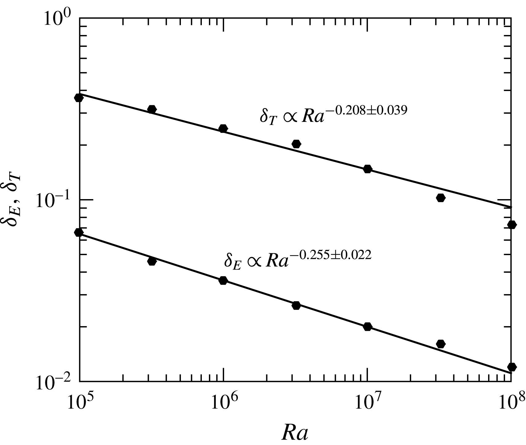
As the Rayleigh number is increased, the boundary layers adjacent to the disks become thinner. Figure 7 shows how the 99 %-thicknesses of the thermal (
 $\unicode[STIX]{x1D6FF}_{T}$
) and Ekman (
 $\unicode[STIX]{x1D6FF}_{E}$
) boundary layers vary with the Rayleigh number, considering
 $k=5$
, as well as a power-law fit with 95 % confidence intervals for the exponents of the two curves. We note that these thicknesses are normalised with respect to the cavity axial length and that they are evaluated at the mid-radial position. As shown qualitatively in figure 5(d), the boundary layer thickness varies along the radial direction, especially near the cylindrical walls. In regions away from the mid-radial location, significant departures from the scalings shown in figure 7 were obtained, presumably because of the greater influence of the cylindrical surfaces. The results show that the Ekman layer scales according to
 $\unicode[STIX]{x1D6FF}_{E}\propto Ra^{-0.255\pm 0.022}$
, which is consistent with the expected scaling
 $\unicode[STIX]{x1D6FF}_{E}\propto \unicode[STIX]{x1D6FA}^{-1/2}\propto Ra^{-1/4}$
for an Ekman layer (recall that the Rayleigh number is evaluated in terms of the centrifugal acceleration
 $\unicode[STIX]{x1D6FA}^{2}r_{0}$
). The thermal boundary layer scales as
 $\unicode[STIX]{x1D6FF}_{T}\propto Ra^{-0.208\pm 0.039}$
, which is in agreement with the scaling
 $\unicode[STIX]{x1D6FF}_{T}\propto Ra^{-1/5}$
obtained from a scale analysis and confirmed experimentally by Rossby (Reference Rossby1965), for natural convection over a stationary plate with a horizontal temperature gradient. Rossby (Reference Rossby1965) has shown that this scaling is valid for the plate itself and also for the vertical side wall used in the experiments, which was adiabatic and therefore equivalent to the disks in the present study. The scaling obtained by Rossby also holds for rotating horizontal convection in some regions of the parameter space (see, e.g. Sheard, Hussam & Tsai Reference Sheard, Hussam and Tsai2016), but it should be noted that in such problems the body force is acting normal to the disks, and not parallel to them, as is the case here. Finally, we note that the uncertainty of the exponent of
 $Ra$
for the
 $\unicode[STIX]{x1D6FF}_{T}$
is rather significant, mainly because there might be a change of slope for
 $Ra>10^{7}$
.
Normalised thicknesses of the thermal (
 $\unicode[STIX]{x1D6FF}_{T}$
) and Ekman (
 $\unicode[STIX]{x1D6FF}_{E}$
) boundary layers as the Rayleigh number is increased, obtained from linear stability analysis for
 $k=5$
. The markers indicate computed solutions and the solid lines represent power-law extrapolations.

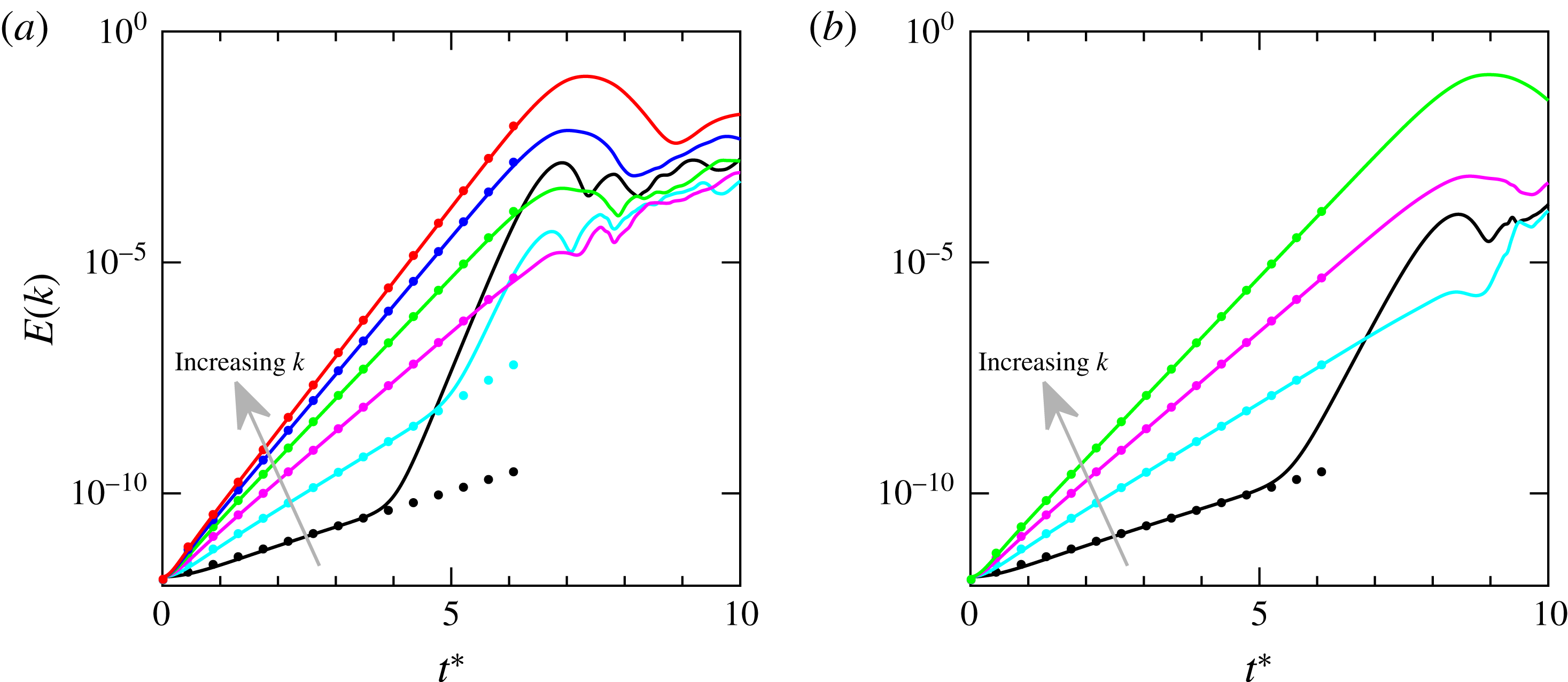
Behaviour of the modal energies when the solution is initialised adding sinusoidal perturbations of wavenumber (a) one to six and (b) one to four, for
 $Ra=10^{8}$
. The solid lines represent the energies obtained from the DNS, and the markers indicate the growth rate obtained from linear stability analysis.

4 Transition to the nonlinear regime
Above the critical Rayleigh number
 $Ra_{c}$
, infinitesimal perturbations grow exponen- tially in time, up to a point where the energy level saturates and the flow transitions to a different state, which can be either quasi-periodic in time or turbulent, depending on the value of
 $Ra$
. To understand how modes with different azimuthal wavenumbers interact before and during the transition process, we perturb the base flow given by (3.1) adding small-amplitude sinusoidal perturbations of the form
 $\sin (k\unicode[STIX]{x1D703})$
to the temperature field. Figure 8 illustrates the behaviour of modal energies when perturbations of wavenumber, ranging from one to six and one to four, are added to the base flow. When six modes are perturbed, the energies of modes three to six grow exponentially with a constant growth rate until the energy level saturates. As indicated by the markers, the growth rates observed for each mode match those calculated from the linear stability analysis. Modes one and two, on the other hand, experience a sudden change in their growth rates before the transition takes place. To investigate why this happens, a case in which only modes one and two are perturbed was run. For that case, no change in the growth rate was observed before the transition for modes one and two. This indicates that the changes in growth rate arise from the nonlinear interactions between the modes. Specifically, mode
 $k=1$
, for instance, interacts with pairs of modes with wavenumbers
 $(n,n+1)$
, where
 $n$
is arbitrary, whilst mode
 $k=2$
interacts with pairs
 $(n,n+2)$
. These triadic interactions are responsible for the behaviour observed for modes one and two in figure 8(a). Mode
 $k=1$
is mostly affected by modes
 $k=5$
and
 $k=6$
, as these have the greatest energies, and its growth rate at
 $t^{\ast }=5$
is approximately given by
 $\unicode[STIX]{x1D706}_{r}(k=6)+\unicode[STIX]{x1D706}_{r}(k=5)$
(this relation is not exact since the growth rate is also affected by interactions between lower-energy modes). Analogously, mode
 $k=2$
is mostly affected by modes
 $k=6$
and
 $k=4$
, and that is why its growth rate after
 $t^{\ast }=5$
is slightly smaller than that for
 $k=1$
. To illustrate this behaviour further, figure 8(b) shows the evolution of modal energies when modes one to four are perturbed. This excludes not only the triad formed by modes
 $k=2$
,
 $k=4$
and
 $k=6$
but also the lowest possible triad for
 $k=2$
, i.e. that with modes
 $k=3$
and
 $k=5$
, while retaining a number of possible triads with
 $k=1$
. Note that in this case mode
 $k=1$
interacts with modes
 $k=4$
and
 $k=3$
and its growth rate increases, whilst no change is observed for mode
 $k=2$
. This shows that the energy growth observed for the lower modes comes from the triadic interactions, and not from a resonance involving subharmonics. It is important to note that although we have observed a significant effect of triadic interactions during transition, we have not identified triadic resonances. Triadic resonances have been observed in experiments of the baroclinic annulus (e.g. Früh & Read (Reference Früh and Read1997), and Früh (Reference Früh, von Larcher and Williams2014) and references therein) and in other rotating systems, such as precessing cylinder flow (Albrecht et al.
Reference Albrecht, Blackburn, Lopez, Manasseh and Meunier2015).
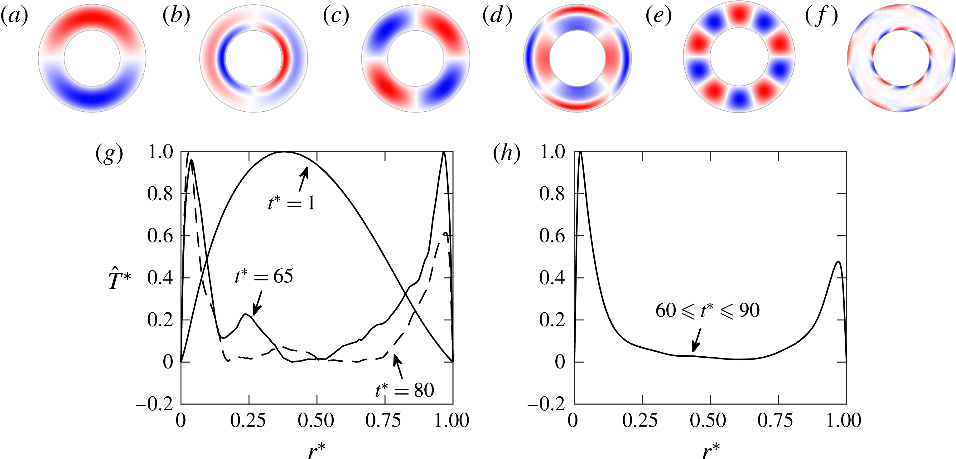
The mode shape associated with each of the perturbed azimuthal modes is similar to that shown in figure 5(b,c), where the number of pairs of cells changes with the mode number. These modes are all associated with modes that have no change of sign in the radial direction, as there is a single cell spanning the radial extent of the cavity. When triadic interactions occur and affect the growth rate of a specific mode, the original mode with a single cell in the radial direction is replaced, as shown in figure 9 for the case where modes one to six are perturbed. In panel (a) of this figure, the shape of mode
 $k=1$
at
 $t^{\ast }=1$
is shown, and panel (b) shows the mode shape at
 $t^{\ast }=5.4$
. These mode shapes were obtained from a Fourier decomposition of the temperature field and are evaluated at the mid-axial position. The modified shape has one change of sign along the radial direction, and the position of the convection cells is shifted when compared to figure 9(a). A similar behaviour is observed for mode
 $k=2$
, as shown in figure 9(c,d). Both the phase shift and the appearance of an extra cell in the radial direction are due to the form of the advection term of the energy equation,
 $\boldsymbol{u}\boldsymbol{\cdot }\unicode[STIX]{x1D735}T$
. Recalling that
 $\sin (\unicode[STIX]{x1D703}_{1})\sin (\unicode[STIX]{x1D703}_{2})=[\cos (\unicode[STIX]{x1D703}_{1}-\unicode[STIX]{x1D703}_{2})-\cos (\unicode[STIX]{x1D703}_{1}+\unicode[STIX]{x1D703}_{2})]/2$
, we see that when two modes interact they give rise to a new wave which is shifted by
 $90^{\circ }$
relative to the original waves. Therefore, the phase shift is
 $\unicode[STIX]{x03C0}/2k$
radians, which is observed in figure 9. This means that both interacting waves have the same phase, which is expected since their drift velocities are small and they were initialised with the same phase. The appearance of an extra cell in the radial direction comes directly from the multiplication of
 $\boldsymbol{u}$
by the temperature gradient, as the initial ‘half-wave’ in the radial direction is multiplied by its derivative, which will also be shifted by
 $90^{\circ }$
.
Temperature contours at the mid-axial position for
 $Ra=10^{8}$
, (a)
 $k=1$
at
 $t^{\ast }=1$
, (b)
 $k=1$
at
 $t^{\ast }=5.4$
, (c)
 $k=2$
at
 $t^{\ast }=1$
, (d)
 $k=2$
at
 $t^{\ast }=6.5$
, (e)
 $k=5$
at
 $t^{\ast }=1$
and (f)
 $k=5$
at
 $t^{\ast }=65$
(turbulent regime). (g) Temperature in Fourier space as a function of the radial position for
 $k=5$
at
 $t^{\ast }=1$
,
 $t^{\ast }=65$
and
 $t^{\ast }=80$
(the curves are normalised with respect to the maximum values of
 $\hat{T}$
). (h) Temperature in Fourier space for
 $k=5$
averaged in the interval
 $60\leqslant t^{\ast }\leqslant 90$
.

After the transition for
 $Ra=10^{8}$
, all the initially perturbed modes retain a certain magnitude and the modal energies decrease as
 $k$
increases, as shown in figure 3(b). Even though a detailed analysis of the turbulent regime is not intended in this work, we have obtained solutions for a few dozen revolutions in the nonlinear regime to observe the behaviour of the flow pattern. The calculations revealed that at
 $t^{\ast }\approx 40$
the mode
 $k=5$
became the dominant mode, despite the fact that its amplification was initially lower than that of mode
 $k=6$
, cf. figure 10(a). As shown by the linear stability analysis, the onset of convection occurs for a critical azimuthal wavenumber
 $k_{c}=5$
. Even though the flow is fully turbulent after the transition at
 $Ra=10^{8}$
, the structure of mode
 $k=5$
is well defined, consisting of two cells attached to the two cylindrical surfaces and separated by a nearly isothermal core, as shown in figure 9(f). Figure 9(g) shows the temperature profile for mode
 $k=5$
in Fourier space as a function of the normalised radial coordinate
 $r^{\ast }$
at three instants. At
 $t^{\ast }=1$
(figure 9
e) the profile consists of a single convection cell, whilst at
 $t^{\ast }=65$
(figure 9
f) there are two cells. At different time instants in the turbulent regime, the mode shape is qualitatively similar, as can be observed by comparing the profiles for
 $t^{\ast }=65$
and
 $t^{\ast }=80$
. Figure 9(h) shows a time average, still for
 $k=5$
, obtained within the interval
 $60\leqslant t^{\ast }\leqslant 90$
. This mode shape provides a good qualitative representation of the expected behaviour of the temperature in the turbulent regime, where the gradients are confined to thin boundary layers near the cylindrical surfaces, with little activity in the cavity core.
(a) Behaviour of the most energetic modes after the transition for
 $Ra=10^{5}$
and
 $Ra=10^{8}$
. (b) Energy spectrum for
 $Ra=10^{5}$
.

It is instructive to compare the flow behaviour observed in the nonlinear regime for
 $Ra=10^{8}$
with a case of lower
 $Ra$
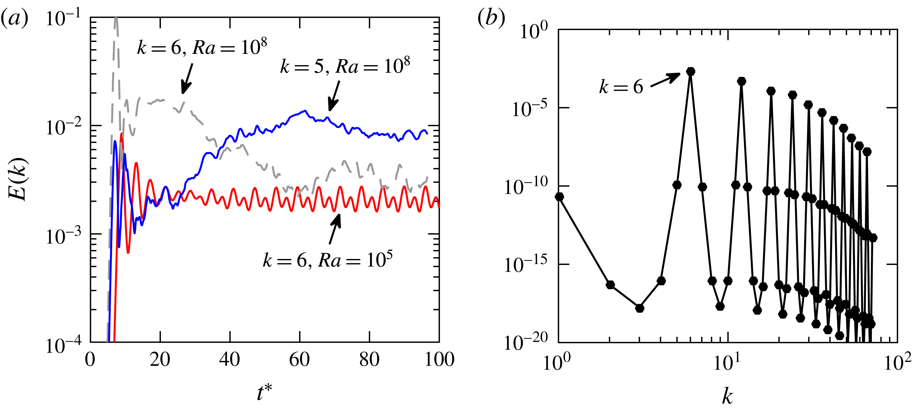
. Figure 10(a) shows how the energy of mode
 $k=6$
behaves after the transition for
 $Ra=10^{5}$
. It is clear from this figure that at this Rayleigh number the flow is quasi-periodic, in contrast with the chaotic behaviour observed for
 $Ra=10^{8}$
. Note that figure 10(a) also shows, for comparison purposes, the corresponding behaviour of modes
 $k=5$
and
 $k=6$
for
 $Ra=10^{8}$
. Another striking difference between the solutions is that for
 $Ra=10^{5}$
modes
 $k=1$
to
 $k=5$
are damped and the harmonics of the dominant mode
 $k=6$
are amplified, reaching significant amplitudes. This behaviour is shown in figure 10(b), which was obtained from a time average comprising several revolution periods, and is in contrast with that observed in figure 3(b) for
 $Ra=10^{8}$
(note that the calculation for
 $Ra=10^{5}$
was run using
 $N_{\unicode[STIX]{x1D703}}=144$
). In this case it is clear that the initial forcing affects the observed periodic behaviour. When the flow is turbulent, on the other hand, the modes interact more intensely and effects related to the initial disturbances tend to disappear more quickly over time.
To further illustrate the behaviour of the solutions obtained for
 $Ra=10^{5}$
and
 $Ra=10^{8}$
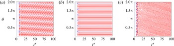
, figure 11 shows azimuth–time plots of the temperature at the mid-axial and mid-radial position. For
 $Ra=10^{5}$
the flow pattern clearly consists of six cells in the azimuthal direction, which are drifting relative to the rotating frame in a direction opposite to that of the cavity rotation. The quasi-periodic nature of the solution is also revealed by the oscillations occurring over time, which indicate that the convection cells move back and forth along the azimuthal direction. As mentioned, the drift of the cells is caused by the end walls (disks), which force the flow to be three-dimensional. To verify whether the limit-cycle oscillation observed for
 $Ra=10^{5}$
is affected by the disks, a calculation was run using a periodicity condition along the axial direction. The corresponding azimuth–time diagram obtained is shown in figure 11(b), which reveals that no drift occurs, as expected, and also that the azimuthal oscillations of the convection cells are quickly damped after the solution saturates. When
 $Ra=10^{8}$
the pattern is much less clear and is dominated by high frequency oscillations, and the cells drift at a faster rate when compared to the lower
 $Ra$
case. Still, the figure reveals that a similar pattern is repeated five times, which is consistent with the fact that
 $k=5$
is the dominant mode. For both values of
 $Ra$
, the drift rates obtained from the linear stability analysis are much smaller than those observed in the nonlinear regime, which indicates that nonlinear effects contribute significantly to the motion of the convection cells relative to the walls.
Space–time plots of temperature at mid-radius and mid-axial position for (a)
 $Ra=10^{5}$
with end walls; (b)
 $Ra=10^{5}$
without end walls; (c)
 $Ra=10^{8}$
with end walls. The temperatures range from
 $T_{a}$
to
 $T_{b}$
.

Temporal evolution of the temperature field at the mid-axial position for (a–f)
 $Ra=10^{5}$
and (g–l)
 $Ra=10^{8}$
. For
 $Ra=10^{5}$
the snapshots are for
 $t^{\ast }=8$
, 9, 10, 12, 24.6 and 27.7, respectively, and for
 $Ra=10^{8}$
 $t^{\ast }=6$
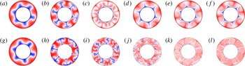
, 7, 8.7, 10, 15 and 60, respectively, so that the instants before, during and after the saturation are covered.

Figure 12 shows that the onset of convection initially follows a similar route for both
 $Ra=10^{5}$
and
 $Ra=10^{8}$
. As the flow loses stability, the hot (cold) jet penetrates radially towards the inner (outer) part of the cavity. For
 $Ra=10^{5}$
the solution quickly becomes a limit cycle and little mixing occurs, whilst for
 $Ra=10^{8}$
the flow becomes turbulent rather abruptly. The initially thin and laminar jets of cold fluid moving outwards lose their stability and become much thicker and chaotic, as shown in figure 12(i), before a fully turbulent state with strong mixing is attained, cf. figure 12(k,l). Note that in figure 12(l), which corresponds to
 $t^{\ast }=60$
,
 $k=5$
has become the dominant mode. Figure 12(e,f) correspond to two extrema of the limit cycle observed for
 $Ra=10^{5}$
; in the first case the cold jets are close to the hot jets located on their right, and in the other extreme the cold jets have moved leftwards. This oscillatory behaviour is repeated indefinitely after the transition, cf. figure 11(a).
5 Conclusions
The problem of convection induced by centrifugal buoyancy in a sealed rotating annulus bounded by horizontal disks was investigated numerically using linear stability analysis and DNS. From the linear analysis predictions were obtained for the critical azimuthal wavenumber and critical Rayleigh number for different radius ratios. The assumption that the azimuthal length of convection cells at the onset of the instability is equal to the radial gap leads to a simple expression which gives an excellent prediction for the critical wavenumber as a function of the radius ratio. Although the disks have only a small effect on the growth rates, especially at large
 $Ra$
, they prevent the flow from being two-dimensional and allow the convection columns to drift, which is associated with the eigenvalues having a non-zero imaginary part. The drift rates observed in the nonlinear regime for
 $Ra=10^{5}$
and
 $Ra=10^{8}$
are much larger than those obtained from the linear analysis. The linear analysis also revealed that the scaling obtained for the Ekman layer is consistent with the expected behaviour
 $\unicode[STIX]{x1D6FF}_{E}\propto \unicode[STIX]{x1D6FA}^{-1/2}$
, and that the thermal boundary layer scales approximately as
 $\unicode[STIX]{x1D6FF}_{T}\propto Ra^{-1/5}$
, which could have an impact on disk heat transfer predictions for cases in which the disks are not thermally insulated.
Our nonlinear analyses consisted of superposing a number of small-amplitude sinusoidal perturbations to the initially stratified temperature field. While some of the modes corresponding to the perturbed wavenumbers grow exponentially with a constant growth rate up to the point where the energy saturates, lower modes are affected by triadic interactions and are more amplified than the other, non-interacting modes. For
 $Ra=10^{5}$
the solutions obtained in the nonlinear regime were shown to be dependent on the initial conditions for the time period considered, as the flow structure is dominated by the initially fastest growing mode and its harmonics. The solution in this case develops limit-cycle oscillations and consists of well-defined convection columns which drift relative to the rotating frame. The columns span the entire axial extent of the cavity, and are slanted near the disks. For
 $Ra=10^{8}$
, effects of the initial perturbation disappear over time and the dominant mode is associated with an azimuthal wavenumber consistent with the critical wavenumber obtained from the linear stability analysis. Although this agreement is reasonable, it is necessary to verify whether it holds at different
 $Ra$
in the turbulent regime and if it persists even at very long integration periods. The fact that the flow is nearly invariant along the axial direction suggests that the use of a two-dimensional model could be appropriate to investigate the flow dynamics in the turbulent regime with a reduced computational cost, although such approach would exclude features such as the drift of the convection columns from the analysis. For
 $Ra=10^{5}$
, the calculations revealed that the presence of the disks not only causes the convection columns to drift, but it also triggers a limit-cycle oscillation, which is not observed in the calculation without the disks.
Read et al. (Reference Read, Maubert, Randriamampianina and Früh2008) have shown that when the Taylor number is increased progressively while keeping the temperature difference constant, the transition to chaos follows a different route depending on whether the flow is dominated by the baroclinic instability or by convection due to the centrifugal force. While for the baroclinic instability the transition occurs via a sequence of low-dimensional states, for
 $Fr>1$
the large-scale motion develops small-scale oscillations when
 $Ta$
is increased. In this work we have isolated the effect of centrifugal buoyancy by neglecting the gravitational acceleration, and have shown the mechanism for the onset of convection and the existence of solutions dominated by a single azimuthal wavenumber and its harmonics, as well as a solution in which the flow is turbulent but still has a clear signature of a certain wavenumber (
 $k=5$
). A natural extension of this work will consist on studying the route to chaos via a gradual increase of the centrifugal Rayleigh number, and seeing whether the transition to chaos occurs directly via the excitation of small scales, as suggested by Read et al. (Reference Read, Maubert, Randriamampianina and Früh2008), or if low-dimensional mechanisms can also occur. Neglecting the effect of gravity is an effective way to study such a transition mechanism, since the flows can be analysed at low Taylor numbers while still neglecting effects arising due to the baroclinic instability. The results presented here also serve as a first step towards fundamental investigations of rotating cavity flows including inlets and outlets, which could be in the form of a radial inflow and axial outflow, or of an axial through flow, both of which are relevant in gas turbine applications. In such cases the flow loses its nearly homogeneous character in the axial direction and the dynamics becomes even more complex.
Acknowledgements
D.B.P. acknowledges the financial support from Capes foundation through the Science without Borders programme and H. Blackburn for developing the numerical tools used in this work.