
1. Introduction
Many fish swim by taking a combination of an active bursting phase and a passive coasting phase, known as burst-and-coast swimming, or intermittent swimming. The advantage of intermittent swimming has been connected to fatigue recovery when coasting without energy consumption, and the amount of energy consumption required to travel a unit distance can be reduced by utilizing intermittent swimming (Videler & Weihs Reference Videler and Weihs1982; Kramer & McLaughlin Reference Kramer and McLaughlin2001; Fish Reference Fish2010). Examples observed in nature include northern anchovy (Weihs Reference Weihs1980), golden shiner (Fish, Fegely & Xanthopoulos Reference Fish, Fegely and Xanthopoulos1991), koi carp (Wu, Yang & Zeng Reference Wu, Yang and Zeng2007), cod (Videler Reference Videler1981; Blake Reference Blake1983) and zebrafish (Fuiman & Webb Reference Fuiman and Webb1988; Müller, Stamhuis & Videler Reference Müller, Stamhuis and Videler2000; McHenry & Lauder Reference McHenry and Lauder2005). In addition, when collections of fish travel in a fluid, the locomotion of each is affected by the others through flow-mediated interactions among them, and individuals in a school can gain an energetic benefit in terms of hydrodynamics (Weihs Reference Weihs1973; Hemelrijk et al. Reference Hemelrijk, Reid, Hildenbrandt and Paddling2015). Although experimental and numerical studies for the collective behaviours of rigid and flexible fins have been conducted using a continuous swimming style (Zhu, He & Zhang Reference Zhu, He and Zhang2014a; Ramananarivo et al. Reference Ramananarivo, Fang, Oza, Zhang and Ristroph2016; Park & Sung Reference Park and Sung2018; Peng, Huang & Lu Reference Peng, Huang and Lu2018; Jeong, Lee & Park Reference Jeong, Lee and Park2021; Lin et al. Reference Lin, Wu, Zhang and Yang2021), there has been little effort to study schooling fins with an intermittent swimming style.
Earlier studies of intermittent swimming by a single fish have found energy savings based on the Bone–Lighthill boundary layer thinning hypothesis (Weihs Reference Weihs1974, Reference Weihs1980; Videler & Weihs Reference Videler and Weihs1982; Wu et al. Reference Wu, Yang and Zeng2007), which holds that a fish can reduce its skin friction drag by interspersing the coast phase between the burst phases because the skin friction drag increases during the burst phase due to the thinning of the boundary layer on the fish body (Lighthill Reference Lighthill1971). Based on this hypothesis, Weihs (Reference Weihs1974, Reference Weihs1980) and Videler & Weihs (Reference Videler and Weihs1982) theoretically predicted the energy savings of an intermittent swimmer. In addition, Wu et al. (Reference Wu, Yang and Zeng2007) performed experiments using intermittently swimming koi carp, demonstrating energy savings based on a vortex ring model to calculate the thrust force acting on the fish. On the other hand, numerical simulations of the intermittent swimming of a single self-propelled rigid/flexible fin have also been performed recently (Chung Reference Chung2009; Akoz & Moored Reference Akoz and Moored2018; Dai et al. Reference Dai, He, Zhang and Zhang2018a; Akoz et al. Reference Akoz, Han, Liu, Dong and Moored2019; Liu, Huang & Lu Reference Liu, Huang and Lu2020). Akoz & Moored (Reference Akoz and Moored2018) simulated a single pitching rigid fin in an inviscid flow, and showed energetic savings by intermittent swimming by calculating the amount of the cost of transport (COT), referring to the energy required to travel a unit distance during one cycle period. A numerical study by Chung (Reference Chung2009) for an airfoil-shaped rigid fin intermittently oscillating by a travelling waveform found an optimal ratio of the chord length over the thickness of the fin for maximum savings of the COT. Furthermore, Dai et al. (Reference Dai, He, Zhang and Zhang2018a) and Liu et al. (Reference Liu, Huang and Lu2020) simulated a single flexible fin with heaving and/or pitching motions, showing that the value of the COT of the fin during intermittent swimming is smaller than that during continuous swimming at an identical cruising speed when the values of the duty cycle (DC) and bending rigidity of the fin are moderate. Although it has been reported that for a single self-propelled swimmer, the intermittent swimming style is more beneficial than the continuous swimming style (Chung Reference Chung2009; Akoz & Moored Reference Akoz and Moored2018; Dai et al. Reference Dai, He, Zhang and Zhang2018a; Akoz et al. Reference Akoz, Han, Liu, Dong and Moored2019; Liu et al. Reference Liu, Huang and Lu2020), no previous work has examined the hydrodynamic benefits of schooling fins utilizing intermittent swimming.
In order to investigate a general principle of fish schooling, the propulsive performance of two tethered rigid and flexible fins with heaving and/or pitching motions under continuous swimming has been studied extensively either in a tandem configuration (Boschitsch, Dewey & Smits Reference Boschitsch, Dewey and Smits2014; Lua et al. Reference Lua, Zhang, Lim and Yeo2016; Muscutt, Weymouth & Ganapathisubramani Reference Muscutt, Weymouth and Ganapathisubramani2017; Kurt & Moored Reference Kurt and Moored2018; Cong, Teng & Cheng Reference Cong, Teng and Cheng2020) or a side-by-side configuration (Dong & Lu Reference Dong and Lu2007; Dewey et al. Reference Dewey, Quinn, Boschitsch and Smits2014; Raj & Arumuru Reference Raj and Arumuru2020). In the tandem configuration with two tethered rigid and flexible fins, a hydrodynamic performance (e.g. thrust and propulsive efficiency) enhancement of an upstream fin was achieved with a short horizontal gap distance between the two fins (Boschitsch et al. Reference Boschitsch, Dewey and Smits2014; Cong et al. Reference Cong, Teng and Cheng2020), and the influence of the downstream fin on the upstream fin is attenuated as the horizontal gap distance increases (Boschitsch et al. Reference Boschitsch, Dewey and Smits2014; Muscutt et al. Reference Muscutt, Weymouth and Ganapathisubramani2017; Cong et al. Reference Cong, Teng and Cheng2020). Compared with an isolated fin, the downstream fin under continuous swimming can outperform or underperform depending on the horizontal gap distance and phase difference between the two tandem fins due to the significant influence of vortices generated by the upstream fin (Boschitsch et al. Reference Boschitsch, Dewey and Smits2014; Lua et al. Reference Lua, Zhang, Lim and Yeo2016; Muscutt et al. Reference Muscutt, Weymouth and Ganapathisubramani2017; Kurt & Moored Reference Kurt and Moored2018; Cong et al. Reference Cong, Teng and Cheng2020). In the side-by-side configuration, the lateral interference induced by mutual interaction between two rigid fins can improve the propulsive performance of the fins (Dong & Lu Reference Dong and Lu2007; Dewey et al. Reference Dewey, Quinn, Boschitsch and Smits2014; Raj & Arumuru Reference Raj and Arumuru2020). When the oscillating motion of two rigid fins was in phase, two side-by-side fins reduced the necessary input power. On the other hand, the thrust force acting on the fins was enhanced when the oscillating motion of two rigid fins was anti-phase. Correspondingly, the schooling efficiency of side-by-side fins both during in-phase and anti-phase oscillations was enhanced compared with that of a single fin. As the lateral gap distance between two rigid fins decreased, the thrust force acting on the fins increased during anti-phase oscillation, whereas the input power of the fins decreased during in-phase oscillation (Dong & Lu Reference Dong and Lu2007; Dewey et al. Reference Dewey, Quinn, Boschitsch and Smits2014).
Because the positions of oscillating rigid and flexible fins in a tethered system do not change when they immediately react to the surrounding flow, self-propelled rigid and flexible models with heaving motions to reflect the reality of the collective dynamics have been employed in tandem (Zhu et al. Reference Zhu, He and Zhang2014a; Ramananarivo et al. Reference Ramananarivo, Fang, Oza, Zhang and Ristroph2016; Park & Sung Reference Park and Sung2018; Jeong et al. Reference Jeong, Lee and Park2021) and side-by-side configurations (Peng et al. Reference Peng, Huang and Lu2018). In a tandem configuration of two self-propelled rigid and flexible fins, the follower spontaneously maintained an equilibrium horizontal gap distance by intercepting a reverse von Kármán vortex street generated by the leader; several equilibrium gap distances were found according to the initial gap distance (Zhu et al. Reference Zhu, He and Zhang2014a; Ramananarivo et al. Reference Ramananarivo, Fang, Oza, Zhang and Ristroph2016; Park & Sung Reference Park and Sung2018; Jeong et al. Reference Jeong, Lee and Park2021). The performance enhancement of the follower in the tandem configuration was maximized at the smallest equilibrium gap distance (Park & Sung Reference Park and Sung2018). In a side-by-side configuration, Peng et al. (Reference Peng, Huang and Lu2018) performed simulations of two self-propelled flexible fins with heaving motion under in-phase and anti-phase oscillations and found that three stable configurations (i.e. the staggered-following mode, alternate-leading mode and moving abreast mode) are spontaneously formed as a result of flow-mediated interactions. When the bending rigidity of the fins was moderate and the lateral gap distance between them was small, the fins achieved high propulsive efficiency in both in-phase and anti-phase oscillations. On the other hand, a very recent numerical study by Lin et al. (Reference Lin, Wu, Zhang and Yang2021) considered two self-propelled pitching rigid fins in a side-by-side configuration that are free to move in both horizontal and lateral directions. They found that freely movable fins with in-phase and anti-phase oscillations can simultaneously move to horizontal and lateral equilibrium gap distances and that a performance enhancement of the fins is achieved at these equilibrium gap distances.
The objective of the present study is to investigate the lateral stability and schooling performance of two self-propelled flexible fins with laterally constrained heaving motions during intermittent swimming. In particular, we consider a side-by-side configuration with anti-phase oscillation because (i) the maximum energy saving of schooling fish is obtained when they swim with anti-phase tail motions (Weihs Reference Weihs1973), and (ii) actual fish pairs favour the anti-phase flapping state (Ashraf et al. Reference Ashraf, Godoy-Diana, Halloy, Collignon and Thiria2016). Motivated by a previous study of two side-by-side fins with continuous swimming (Lin et al. Reference Lin, Wu, Zhang and Yang2021), the lateral stability of the fins during intermittent swimming, which is an essential condition for maintaining the schooling formation, is studied first to resolve two main questions: (i) whether there exists an equilibrium lateral gap distance between two side-by-side fins during intermittent swimming, and (if so) (ii) how fins during intermittent swimming maintain the lateral stability. We show that an equilibrium lateral gap distance between two self-propelled side-by-side flexible fins for intermittent swimming gait exists and that stable equilibrium states for intermittent swimming can arise at smaller and larger lateral gap distances depending on the intermittent swimming style than that for continuous swimming. A control volume analysis in the lateral direction to investigate a physical mechanism leading to stable states for intermittent swimming shows that an added-mass lateral force related to asymmetric flapping kinematics by passive flexibility plays an important role to determine the lateral stability of two fins in addition to circulatory lateral forces due to jet deflection and enhanced positive pressure between the fins. When the cruising speed or the cycle-averaged input power is identical between continuous and intermittent swimming in a stable state, we find that the COT value of the two fins for intermittent swimming is significantly reduced compared with that for continuous swimming. Finally, we show the distinctive role of passive flexibility on the schooling performance in intermittent swimming compared with continuous swimming.
2. Numerical method
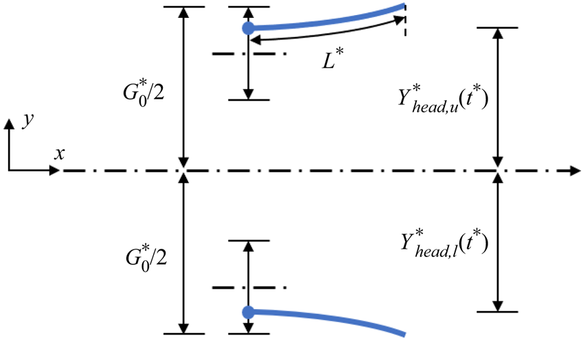
Figure 1 shows a schematic of two self-propelled flexible fins in a side-by-side configuration for collective locomotion. The initial lateral gap distance between the positions of the leading edges (head) for the upper and lower fins is denoted by  $G_0^\ast $, where the superscript * indicates a dimensional parameter. Two flexible upper and lower fins are actively forced by laterally constrained heaving motion at the leading edge (i.e.
 $Y_{head,u}^\ast $ and
 $Y_{head,l}^\ast $, where the subscripts u and l denote the upper and lower fins) and as a result, the fins are free to move in the horizontal direction.
Schematic of two self-propelled flexible fins in a side-by-side configuration. The initial lateral gap distance between the positions of the leading edges for the upper and lower fins is denoted by  $G_0^\ast $. When the leading edges of the fins are forced to heave laterally, i.e.
 $Y_{head,u}^\ast ({t^\ast })$ and
 $Y_{head,l}^\ast ({t^\ast })$, the fins are free to move in the horizontal direction.

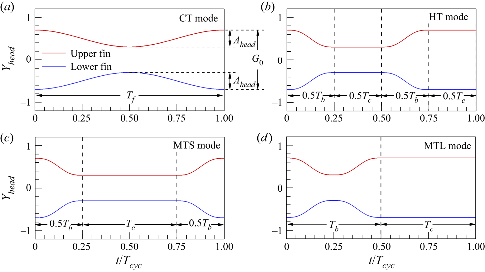
Figure 2 shows the time histories for the dimensionless lateral position of the leading edge  $({Y_{head}} = Y_{head}^\ast{/}{L^\ast })$ for the upper and lower fins during continuous and intermittent swimming under anti-phase oscillation (ϕ =
 ${\rm \pi}$) when
 ${G_0} = G_0^\ast{/}{L^\ast } = 1.4$, where L* is the fin length. In the figure,
 ${A_{head}}( = A_{head}^\ast{/}{L^\ast })$ is the peak-to-peak heaving amplitude and
 ${T_f}( = T_f^\ast U_{ref}^\ast{/}{L^\ast })$,
 ${T_b}( = T_b^\ast U_{ref}^\ast{/}{L^\ast })$,
 ${T_c}( = T_c^\ast U_{ref}^\ast{/}{L^\ast })$ and Tcyc (=Tb + Tc) are the flapping, bursting, coasting and total cycle periods, respectively (here,
 $U_{ref}^\ast $ is the reference velocity). In the continuous-tail-beating (CT) mode (Liu et al. Reference Liu, Huang and Lu2020) in figure 2(a), the harmonic lateral motion of the leading edge for the upper fin during the flapping period is prescribed as follows:
 \begin{equation}{Y_{head,u}}(t) = \frac{{{A_{head}}}}{2}\cos (2{\rm \pi} {f_f}t) - \frac{{{A_{head}}}}{2} + \frac{{{G_0}}}{2},\end{equation}
where ff (=1/Tf) is the flapping frequency and t is the time. For all cases of two anti-phase flapping fins in continuous and intermittent swimming, the prescribed lateral motion of the leading edge for the lower fin is symmetric relative to that of the upper fin with respect to the centreline; i.e. Yhead,l(t) = −Yhead,u(t) (figure 2). In figure 2(b–d), two intermittent swimming modes, i.e. the half-tail-beating (HT) mode and the multiple-tail-beating (MT) mode, are adopted for actuation at the leading edge (Wu et al. Reference Wu, Yang and Zeng2007; Chung Reference Chung2009; Dai et al. Reference Dai, He, Zhang and Zhang2018a; Liu et al. Reference Liu, Huang and Lu2020). For the HT mode, active bursting and passive coasting are divided in half and each period is interspersed alternatively (figure 2b). The lateral motion of the leading edge of the upper fin for the HT mode is expressed as follows:
 \begin{equation}{Y_{head,u}}(t) = \left\{ {\begin{array}{*{20}{@{}l}} {\dfrac{{{A_{head}}}}{{2{\rm \pi} }}(\sin (4{\rm \pi} {f_{ref}}t) - 4{\rm \pi} {f_{ref}}t) + \dfrac{{{G_0}}}{2},\quad 0 \le t \le 0.5{T_b};}\\ { - {A_{head}} + \dfrac{{{G_0}}}{2},\quad 0.5{T_b} \le t \le 0.5{T_{cyc}};}\\ \begin{array}{@{}l} - \dfrac{{{A_{head}}}}{{2{\rm \pi} }}(\sin (4{\rm \pi} {f_{ref}}(t - 0.5{T_{cyc}})) - 4{\rm \pi} {f_{ref}}(t - 0.5{T_{cyc}}))\\ \quad - {A_{head}} + \dfrac{{{G_0}}}{2},\quad 0.5{T_{cyc}} \le t \le 0.5{T_{cyc}} + 0.5{T_b}; \end{array}\\ {\dfrac{{{G_0}}}{2},\quad 0.5{T_{cyc}} + 0.5{T_b} \le t \le {T_{cyc}};} \end{array}} \right.\end{equation}
where fref (=1/Tb) is the reference frequency. For the MT mode, one full period of active bursting is arranged before and after that of passive coasting. In a side-by-side configuration, two types of MT modes are possible according to the coast position of the upper and lower fins: coasting at the smallest G in figure 2(c) (hereafter, ‘MTS mode’) and coasting at the largest G in figure 2(d) (hereafter, ‘MTL mode’), where G is the temporal lateral gap distance between the leading edges of the upper and lower fins. The lateral motions of the leading edges for the upper fins for two distinct MTS (2.3) and MTL (2.4) modes are expressed as follows:
 \begin{gather}{Y_{head,u}}(t) = \left\{ {\begin{array}{@{}l} {\dfrac{{{A_{head}}}}{{2{\rm \pi} }}(\sin (4{\rm \pi} {f_{ref}}t) - 4{\rm \pi} {f_{ref}}t) + \dfrac{{{G_0}}}{2},\quad 0 \le t \le 0.5{T_b};}\\ { - {A_{head}} + \dfrac{{{G_0}}}{2},\quad 0.5{T_b} \le t \le 0.5{T_b} + {T_c};}\\ \begin{array}{@{}l} - \dfrac{{{A_{head}}}}{{2{\rm \pi} }}(\sin (4{\rm \pi} {f_{ref}}(t - 0.5{T_b} + {T_c})) - 4{\rm \pi} {f_{ref}}(t - 0.5{T_b} + {T_c}))\\ \quad - {A_{head}} + \dfrac{{{G_0}}}{2},\quad 0.5{T_b} + {T_c} \le t \le {T_{cyc}}, \end{array} \end{array}} \right.\end{gather}
 \begin{gather}{Y_{head,u}}(t) = \left\{ {\begin{array}{@{}l} {\dfrac{{{A_{head}}}}{{2{\rm \pi} }}(\sin (4{\rm \pi} {f_{ref}}t) - 4{\rm \pi} {f_{ref}}t) + \dfrac{{{G_0}}}{2},\quad 0 \le t \le 0.5{T_b};}\\ \begin{array}{@{}l} - \dfrac{{{A_{head}}}}{{2{\rm \pi} }}(\sin (4{\rm \pi} {f_{ref}}(t - 0.5{T_b})) - 4{\rm \pi} {f_{ref}}(t - 0.5{T_b}))\\ \quad - {A_{head}} + \dfrac{{{G_0}}}{2},\,\,\,0.5{T_b} \le t \le {T_b}; \end{array}\\ {\dfrac{{{G_0}}}{2},\quad {T_b} \le t \le {T_{cyc}}.} \end{array}} \right.\end{gather}
In (2.2)–(2.4), smoothed piecewise functions are used to facilitate the natural transition between the burst and the coast phases (Dai et al. Reference Dai, He, Zhang and Zhang2018a). Because two fins are free to move without any constraints in the horizontal (x) direction, the moving (or cruising) speed of the fins is determined spontaneously as a result of fluid–structure interactions. However, the fins cannot move freely in the lateral (y) direction due to the prescribed active motion at the leading edge as shown in (2.1)–(2.4).
Time histories of the lateral position of the leading edge (Yhead) for upper and lower fins with anti-phase oscillation when G 0 = 1.4: (a) CT mode, (b) HT mode and (c,d) MT modes. Here, two types of MT modes are considered when two fins are coasting (c) at the smallest G (MTS mode) and (d) at the largest G (MTL mode). Here, G is the temporal lateral gap distance between the leading edges of the fins. In (a), Ahead is the peak-to-peak heaving amplitude, G 0 is the initial lateral gap distance and Tf is the flapping period. In (b–d), Tb and Tc are the burst and coast periods, respectively.

The motion of an incompressible viscous flow is governed by the Navier‒Stokes and continuity equations
 \begin{gather}\frac{{\partial \boldsymbol{u}}}{{\partial t}} + \boldsymbol{u}\boldsymbol{\cdot }\boldsymbol{\nabla }\boldsymbol{u} ={-} \boldsymbol{\nabla }p + \frac{1}{{Re}}{\nabla ^2}\boldsymbol{u} + \boldsymbol{f},\end{gather}
 \begin{gather}\boldsymbol{\nabla }\boldsymbol{\cdot }\boldsymbol{u} = 0,\end{gather}
where the flapping Reynolds number Re is defined as  $Re = \rho _0^\ast U_{ref}^\ast {L^\ast }/{\mu ^\ast }$ with the dimensional parameters of the fluid density
 $\rho _0^\ast $ and the dynamic viscosity μ*. All quantities in (2.5) and (2.6) are dimensionless:
 $\boldsymbol{u} = {\boldsymbol{u}^\ast }/U_{ref}^\ast $,
 $t = {t^\ast }/({L^\ast }/U_{ref}^\ast )$,
 $p = {p^\ast }/(\rho _0^\ast {(U_{ref}^\ast )^2})$ and
 $\boldsymbol{f} = {\boldsymbol{f}^\ast }/(\rho _0^\ast {(U_{ref}^\ast )^2}/{L^\ast })$ (where u is the velocity, p is the pressure and f is the momentum forcing). Equations (2.5) and (2.6) are integrated in time using the fractional step method with an implicit velocity-decoupling procedure (Kim, Baek & Sung Reference Kim, Baek and Sung2002). Block lower triangular-upper triangular (LU) decomposition with approximate factorization is applied to achieve both velocity–pressure decoupling and decoupling of the intermediate-velocity components. In this approach, the terms are initially discretized in time using the Crank–Nicolson method, after which the coupled velocity components are solved without iterations. Based on a second-order central difference scheme, all terms are resolved in space with a staggered mesh.
The non-dimensional fin motion with an inextensibility condition is described as follows (Huang, Shin & Sung Reference Huang, Shin and Sung2007):
 \begin{gather}\frac{{{\partial ^2}\boldsymbol{X}}}{{\partial {t^2}}} = \frac{\partial }{{\partial s}}\left( {\zeta \frac{{\partial \boldsymbol{X}}}{{\partial s}}} \right) - \frac{{{\partial ^2}}}{{\partial {s^2}}}\left( {\gamma \frac{{{\partial^2}\boldsymbol{X}}}{{\partial {s^2}}}} \right) - {\boldsymbol{F}_L},\end{gather}
 \begin{gather}\frac{{\partial \boldsymbol{X}}}{{\partial s}} \cdot \frac{{\partial \boldsymbol{X}}}{{\partial s}} = 1,\end{gather}
where s is the Lagrangian variable defined along the fin (0 ≤ s ≤ 1) and X = (X(s,t), Y(s,t)) is the position of the fin, γ is the bending rigidity and FL is the Lagrangian momentum force. All quantities in (2.7) and (2.8) are dimensionless:  $\boldsymbol{X} = {\boldsymbol{X}^\ast }/{L^\ast }$,
 $s = {s^\ast }/{L^\ast }$,
 ${\boldsymbol{F}_L} = \boldsymbol{F}_L^\ast{/}(\rho _1^\ast {(U_{ref}^\ast )^2}/{L^\ast })$,
 $\zeta = {\zeta ^\ast }/(\rho _1^\ast {(U_{ref}^\ast )^2})$ and
 $\gamma = {\gamma ^\ast }/(\rho _1^\ast {(U_{ref}^\ast {L^\ast })^2})$ (where
 $\rho _1^\ast $ is the density difference between the flexible fin and the surrounding fluid). The tension force ζ is a function of the time t and the Lagrangian variable s and is determined by the inextensibility condition (2.8). In addition to the constrained conditions in the y-direction ((2.1)–(2.4)), a clamped condition and an unconstrained condition in the x-direction are imposed at the leading edge (s = 0), as follows:
 \begin{equation}\frac{{\partial \boldsymbol{X}}}{{\partial s}} = (1,0),\quad \frac{{{\partial ^3}X}}{{\partial {s^3}}} = 0\ \textrm{at}\ s = 0.\end{equation}
The free-end boundary condition at the trailing edge (s = 1) is given by
 \begin{equation}\zeta = 0,\quad \frac{{{\partial ^2}\boldsymbol{X}}}{{\partial {s^2}}} = (0,0),\quad \frac{{{\partial ^3}\boldsymbol{X}}}{{\partial {s^3}}} = (0,0)\ \textrm{at}\ s = 1.\end{equation}
The Lagrangian momentum force between the fluid and the fin FL in (2.7) is calculated by the feedback force
 \begin{equation}{\boldsymbol{F}_L}(s, t) ={-} \kappa [({\boldsymbol{X}_{ib}} - \boldsymbol{X}) + \varDelta t({\boldsymbol{U}_{ib}} - \boldsymbol{U})],\end{equation}
where κ = 2 × 10⁶ denotes a user-defined constant, Δt = 0.0001 is the computational time step and U = (U(s,t), V(s,t)) estimated by U = ∂X/∂t is the velocity of the fin. In contrast, Xib and Uib denote the position and velocity of the immersed boundary, respectively. These values are obtained from the local Eulerian fluid velocity
 \begin{gather}{\boldsymbol{X}_{ib}} = \boldsymbol{X}_{ib}^0 + \int_0^t {{\boldsymbol{U}_{ib}}\,\textrm{d}t} ,\end{gather}
 \begin{gather}{\boldsymbol{U}_{ib}}(s,t) = \int_{{\varOmega _f}} {\boldsymbol{u}(\boldsymbol{x},t)\delta (\boldsymbol{X}(s,t) - \boldsymbol{x})\,\textrm{d}\boldsymbol{x}} ,\end{gather}
where  $\varOmega_{f}$ denotes the fluid region and δ() denotes the smoothed Dirac delta function. By spreading the Lagrangian force FL to the neighbouring Eulerian grid points, the Eulerian momentum force f is calculated using the smoothed Dirac delta function,
 \begin{equation}\boldsymbol{f}(\boldsymbol{x},t) = \rho \int_{{\varOmega _s}} {{\boldsymbol{F}_L}(s,t)\delta (\boldsymbol{x} - \boldsymbol{X}(s,t))\,\textrm{d}s},\end{equation}
where  $\rho = \rho _1^\ast{/}(\rho _0^\ast {L^\ast })$ is the structure-to-fluid mass ratio and
 $\varOmega_{s}$ denotes the structure region.
The computational domain normalized by the fin length is 81.92 and 20.0 in the x- and y-directions (−40.96 ≤ x ≤ 40.96 and −10.0 ≤ y ≤ 10.0) with a constant grid spacing of 0.02. The number of Lagrangian grids for the fin is 50. Neumann boundary conditions are applied at the entire boundary  $(\partial \boldsymbol{u}/\partial x{|_{x ={-} 40.96,40.96}} = \partial \boldsymbol{u}/\partial y{|_{y ={-} 10,10}} = 0)$. Initially, the fluid is quiescent with zero velocity in the entire computational domain. The numerical method used in the present study has been validated through a direct comparison with previous data for tethered flexible fins (Huang et al. Reference Huang, Shin and Sung2007; Kim, Huang & Sung Reference Kim, Huang and Sung2010; Uddin, Huang & Sung Reference Uddin, Huang and Sung2013, Reference Uddin, Huang and Sung2015; Jeong & Lee Reference Jeong and Lee2017; Son & Lee Reference Son and Lee2017) and self-propelled flexible fins (Park, Kim & Sung Reference Park, Kim and Sung2017; Park & Sung Reference Park and Sung2018; Jeong et al. Reference Jeong, Lee and Park2021), suggesting the reliability and accuracy of our numerical method.
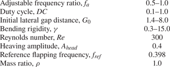
All non-dimensional parameters used in the present study are listed in table 1. Four parameters are varied: the adjustable frequency ratio (fa), the DC, the initial lateral gap distance (G 0) and the bending rigidity (γ). The four remaining parameters of Re, Ahead,fref and ρ are fixed in our simulation. The adjustable frequency ratio is defined as  ${f_a} = f_f^\ast{/}f_{ref}^\ast = {f_f}/{f_{ref}}(0.5 \le {f_a} \le 1)$ to identify the performance of continuous swimmers in a wide range of cruising speeds. Because the reference velocity of
 $U_{ref}^\ast = 2{\rm \pi} f_{ref}^\ast A_{head}^\ast $ is adopted in the present study (Park et al. Reference Park, Kim and Sung2017; Park & Sung Reference Park and Sung2018; Ryu & Sung Reference Ryu and Sung2019), the value of
 ${f_{ref}}( = f_{ref}^\ast {L^\ast }/U_{ref}^\ast = f_{ref}^\ast {L^\ast }/(2{\rm \pi} f_{ref}^\ast A_{head}^\ast ) = 1/(2{\rm \pi} {A_{head}}))$ is fixed at 0.398 when Ahead = 0.4. DC, which represents the degree of intermittency in burst-and-coast swimming, is defined as DC = Tb/(Tb + Tc) = Tb/Tcyc (Chung Reference Chung2009; Akoz & Moored Reference Akoz and Moored2018; Dai et al. Reference Dai, He, Zhang and Zhang2018a; Akoz et al. Reference Akoz, Han, Liu, Dong and Moored2019; Ryu & Sung Reference Ryu and Sung2019; Liu et al. Reference Liu, Huang and Lu2020), and a small DC indicates that an intermittent swimmer takes more rest without energy consumption. It should also be noted that the value of DC for the CT mode is always 1.0, indicating steady swimming without a coast phase during the cycle (i.e. Tcyc = Tf). For intermittent swimming, because the burst period (Tb = 1/fref) is fixed at 2.51, the value of DC varies according to the coast period (Tc). The value of G 0 is selected in the range of 1.4 ≤ G 0 ≤ 8.0 because two flexible fins with anti-phase oscillation in a side-by-side configuration collide each other when G 0 < 1.4 and the mutual interaction between two fins disappears when G 0 > 8.0 in the present parameter settings. The relatively low Reynolds number (Re = 300) employed in the present study can be observed in biological studies for intermittent swimming of, for instance, larval northern anchovy and zebrafish (Weihs Reference Weihs1980; Müller et al. Reference Müller, Stamhuis and Videler2000). Furthermore, the Reynolds number is comparable to the values used in many previous studies of self-propelled flexible fins adopting a continuous swimming gait (Zhu et al. Reference Zhu, He and Zhang2014a; Zhu, He & Zhang Reference Zhu, He and Zhang2014b; Park & Sung Reference Park and Sung2018; Peng et al. Reference Peng, Huang and Lu2018; Jeong et al. Reference Jeong, Lee and Park2021; Lin et al. Reference Lin, Wu, Zhang and Yang2021) and an intermittent swimming gait (Ryu & Sung Reference Ryu and Sung2019; Liu et al. Reference Liu, Huang and Lu2020).
Parameters considered in our simulations.

3. Results and discussion
3.1. Lateral stability
3.1.1. Existence of an equilibrium lateral gap distance
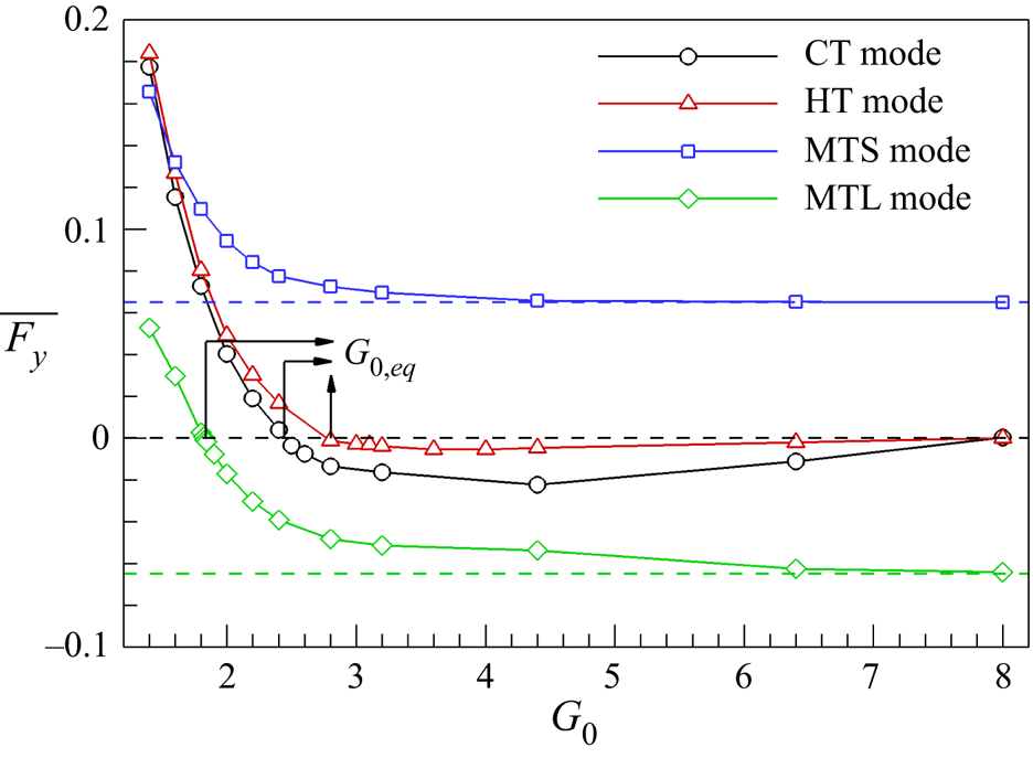
In a side-by-side configuration, it has been known that for continuous swimming, the lateral interference of a nearby fin can enhance the schooling performance and a specific lateral spacing between two side-by-side fins exists to maintain a stable state as a result of flow-mediated interactions between the fins (Lin et al. Reference Lin, Wu, Zhang and Yang2021). However, the existence of the lateral equilibrium position for two side-by-side fins during intermittent swimming is still unclear. The cycle-averaged lateral force  $(\overline {{F_y}} )$ acting on the upper fin for continuous swimming (CT mode) with fa = 1.0 and intermittent swimming (HT, MTS and MTL modes) with DC = 0.5 is analysed in figure 3 as a function of the initial lateral gap distance (G 0) to resolve the following questions: (i) Does an equilibrium lateral gap distance exist between two self-propelled side-by-side flexible fins with unique patterns in intermittent swimming and (if so) (ii) can two fins using a specific type of intermittent swimming reduce the equilibrium lateral gap distance compared with continuous swimming? In this figure, only data for the upper fin are presented because the overall lateral motions of the upper and lower fins are symmetric with respect to the centreline, resulting in identical cycle-averaged lateral forces
 $(\overline {{F_y}} )$ acting on the lower fin with an opposite sign (the overbar denotes the cycle-average value). In addition, the value of γ is set to 1.0. In figure 3, positive values of
 $\overline {{F_y}}$ acting on the upper fin in the CT mode (black circle) and the HT mode (red triangle) are found at small values of G 0, indicating that the fins tend to push each other (away from the centreline). As the value of G 0 increases, the values of
 $\overline {{F_y}}$ acting on the upper fin in the CT and HT modes become negative, and zero values of
 $\overline {{F_y}}$ are found at G 0 = 2.4 for the CT mode and 2.8 for the HT mode, corresponding to the initial lateral gap distance at which an equilibrium stable state is achieved (i.e. G 0,eq). A similar trend of
 $\overline {{F_y}}$ is found on the upper fin for the MTL mode (green diamond). However, the value of G 0,eq for the MTL mode (G 0,eq = 1.82) is smaller than that for the CT mode. On the other hand, the values of
 $\overline {{F_y}}$ acting on the upper fin in the MTS mode (blue square) are always positive regardless of G 0, indicating that two side-by-side flexible fins using this mode cannot achieve a stable propulsion state. At G 0 = 8 for all modes, the values of
 $\overline {{F_y}}$ acting on the upper fin approach those of an isolated fin in each mode (dashed line) with little influence by the lower fin.
Cycle-averaged lateral force  $(\overline {{F_y}} )$ acting on the upper fin with γ = 1.0 as a function of the initial lateral gap distance (G 0) for continuous swimming with fa = 1.0 and intermittent swimming with DC = 0.5: black circle, CT mode; red triangle, HT mode; blue square, MTS mode; green diamond, MTL mode. Here, G 0,eq indicates the initial lateral gap distance at which an equilibrium stable state with
 $\overline {{F_y}} = 0$ is achieved in each mode. Blue and green dashed lines indicate the values of
 $\overline {{F_y}}$ acting on an isolated fin in the MT mode when the fin is coasting at the minimum Yhead and maximum Yhead, respectively. Black dashed line indicates a zero value of
 $\overline {{F_y}}$ acting on a single fin for the CT and HT modes.

In previous experimental and numerical studies, the existence of the lateral equilibrium positions for two side-by-side schooling fins with anti-phase oscillation and for a single fin near the ground has been widely reported when continuously prescribed heaving and/or pitching motions in the y-direction (constrained lateral motion) are adopted while a rigid fin is fixed in the x-direction (i.e. tethered systems) (Quinn et al. Reference Quinn, Moored, Dewey and Smits2014; Zhong et al. Reference Zhong, Han, Moored and Quinn2021) and while flexible fin(s) are free to move in the x-direction (i.e. self-propulsion systems) (Dai, He & Zhang Reference Dai, He and Zhang2016; Zhang, Huang & Lu Reference Zhang, Huang and Lu2017; Dai et al. Reference Dai, He, Zhang and Zhang2018b; Jeong et al. Reference Jeong, Lee and Park2021). It should be noted that flow and pressure fields around the upper fin with anti-phase oscillation in a side-by-side configuration are analogous to those around a single fin near the ground (Dewey et al. Reference Dewey, Quinn, Boschitsch and Smits2014; Zhong et al. Reference Zhong, Han, Moored and Quinn2021). Furthermore, the presence of equilibrium states for two side-by-side anti-phase flapping rigid fins and a single rigid fin near the ground during continuous swimming has been proved in theoretical studies with mathematical expressions for the hydrodynamic forces acting on rigid fin(s) with constrained lateral motions in tethered (Baddoo et al. Reference Baddoo, Kurt, Ayton and Moored2020, Reference Baddoo, Moore, Oza and Crowdy2021) and self-propulsion systems (Oza, Ristroph & Shelley Reference Oza, Ristroph and Shelley2019). Although the models using the constrained lateral motions above are unable to move toward an equilibrium lateral position while reacting to the surrounding fluid, an idealized pure pitching motion of two side-by-side anti-phase flapping rigid fins and a single rigid fin under a ground effect to move freely in the y-direction has shown flow-mediated organization (at equilibrium positions) in the y-direction (Kurt et al. Reference Kurt, Cochran-Carney, Zhong, Mivehchi, Quinn and Moored2019) and in the x- and y-directions (Kurt et al. Reference Kurt, Ormonde, Mivehchi and Moored2021; Lin et al. Reference Lin, Wu, Zhang and Yang2021). However, it should be noted that the propulsive performance in this case is underestimated due to the dynamic recoil motion (i.e. opposite lateral motion of the leading and trailing edges) that occurs (Kurt et al. Reference Kurt, Cochran-Carney, Zhong, Mivehchi, Quinn and Moored2019, Reference Kurt, Ormonde, Mivehchi and Moored2021; Lin et al. Reference Lin, Wu, Zhang and Yang2021). Based on these observations, it is reasonable to infer that the occurrence of equilibrium lateral states is a common phenomenon for two side-by-side anti-phase flapping fins and a single fin near the ground during continuous swimming regardless of the conditions of the model set-up, such as flexibility, moving or stationary conditions and types of active motions. In contrast to continuous swimming, however, although three types of intermittent swimming modes for two fins (MTL, MTS and HT modes) are considered, only the MTL and HT modes can present an equilibrium state, demonstrating that two side-by-side flexible fins in a proper form of intermittent swimming motion can maintain an equilibrium state.
Because the cycle-averaged lateral gap distance between two fins in equilibrium states is affected by the intermittent swimming mode (for example, see the MTS and MTL modes in figure 2), an equilibrium lateral gap distance (Geq) is derived mathematically by averaging the temporal lateral gap distance between the upper and lower fins (G) during the cycle for an equivalent comparison of the lateral equilibrium distances between different modes: Geq = G 0,eq − Ahead for the CT and HT modes, Geq = G 0,eq − AheadDC for the MTL mode and Geq = G 0,eq − AheadDC − 2Ahead for the MTS mode. The values of Geq for the CT, HT and MTL modes are 2.0, 2.4 and 1.62, respectively.
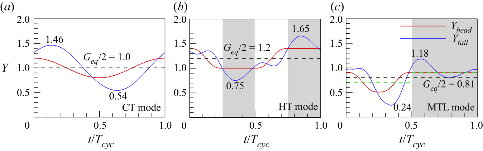
At the equilibrium positions (Geq), the time histories of the lateral position of the leading edge (Yhead) and trailing edge (Ytail) are presented in figure 4 to show the flapping kinematics of the upper fin in each mode. In figure 4(a), the profile of Ytail (blue line) for the upper fin in the CT mode is symmetric with respect to the equilibrium position of the prescribed lateral motion of Yhead (here, Geq/2; see the horizontal black dashed line). It should be noted that the profile of Ytail of two side-by-side flexible fins (or a single flexible fin near the ground) during continuous swimming can be asymmetric when the lateral gap distance between the fins (or from the ground) is reduced (G 0 < Geq) due to the strong influence of a nearby fin (or ground) (Dai et al. Reference Dai, He and Zhang2016; Park et al. Reference Park, Kim and Sung2017). Similar to the CT mode, a symmetric profile of Ytail for the upper fin in the HT mode with respect to Geq/2 can be found in figure 4(b). These results indicate that two side-by-side flexible fins in the CT and HT modes maintain the symmetric flapping kinematics when they achieve a stable lateral state despite the passive response of the fins. In contrast to the observations for the CT and HT modes, two side-by-side flexible fins in the MTL mode, as depicted in figure 4(c), show asymmetric flapping kinematics for Ytail with respect to Geq/2. In addition, the flapping kinematics for the MTL mode is asymmetric even with respect to the equilibrium positions of bursting (green dashed line during 0 ≤ t/Tcyc < 0.5) and coasting (green dashed line during 0.5 ≤ t/Tcyc < 1.0) motions. The inconsistent flapping kinematics between the HT and MTL modes suggests that the symmetric nature of the body response for two side-by-side flexible fins during intermittent swimming is strongly influenced by the coasting position and arrangement (figure 4b,c). In the following sections, a two-fin system in the MTL mode is studied further as a representative of two side-by-side flexible fins during intermittent swimming because it is expected that the smaller value of Geq for the MTL mode than that for the HT mode (figure 3) leads to a performance enhancement of two self-propelled side-by-side flexible fins with anti-phase oscillation (ϕ =  ${\rm \pi}$) (Dai et al. Reference Dai, He and Zhang2016; Park et al. Reference Park, Kim and Sung2017; Zhang et al. Reference Zhang, Huang and Lu2017; Peng et al. Reference Peng, Huang and Lu2018).
Time histories of the lateral position of the leading edge (Yhead) and trailing edge (Ytail) for the upper fin at Geq when γ = 1.0: (a) CT mode with fa = 1.0, (b) HT mode with DC = 0.5 and (c) MTL mode with DC = 0.5. Horizontal black dashed lines indicate half values of Geq in each mode. Two numbers in each mode indicate the maximum and minimum values of Ytail. In (b,c), white and grey regions indicate the burst and coast phases. Green dashed lines during the burst period (0 ≤ t/Tcyc < 0.5) and the coast period (0.5 ≤ t/Tcyc < 1.0) in (c) denote the equilibrium positions of each period for the MTL mode.

3.1.2. Hydrodynamic mechanism leading to lateral stable equilibrium states
In this section, we investigate a hydrodynamic mechanism leading to lateral equilibrium states for two side-by-side flexible fins during the intermittent swimming with a focus on the following two questions: (i) What components play a role in the achievement of a lateral stable state in the MTL mode, and how does the hydrodynamic mechanism leading to lateral equilibrium states for the MTL mode differ from that for the CT mode, and (ii) why is a stable equilibrium state for two flexible fins in the MTL mode achieved at a lateral gap distance smaller than that in the CT mode? To identify the components of the hydrodynamic forces acting on a fin, a control volume (CV) analysis in the y-direction is employed since the force production of flapping fins can be extracted from the velocity and pressure fields within a CV (Kurtulus, Scarano & David Reference Kurtulus, Scarano and David2007; Jardin, David & Farcy Reference Jardin, David and Farcy2009; Shen, Chan & Lin Reference Shen, Chan and Lin2009; Wu et al. Reference Wu, Shu, Wan, Wang and Chen2022). The detailed process of the CV analysis is presented below. The conservation of the momentum in a moving CV is expressed as
 \begin{align}&\frac{\partial }{{\partial {t^\ast }}}\int
\rho _0^\ast \boldsymbol{u}^{\ast}\,\textrm{d}{\forall}^\ast + \oint {({\boldsymbol{n}_{out}} \cdot \rho _0^\ast {\boldsymbol{u}^\ast })({\boldsymbol{u}^\ast } - \boldsymbol{u}_{cv}^\ast )\,\textrm{d}{S^\ast }}\nonumber\\ &\quad ={-} \oint {{p^\ast }{\boldsymbol{n}_{out}}\,\textrm{d}{S^\ast }} + \oint {{\tau ^\ast }{\boldsymbol{n}_{out}}\,\textrm{d}{S^\ast }} - \boldsymbol{F}_L^\ast ,\end{align}
where  ${\forall} ^\ast $ is the CV, S* is the control surface (CS), nout is the outward-facing unit normal vector on the surface,
 $\boldsymbol{u}_{cv}^\ast $ is the velocity of the CV and τ* is the viscous stress tensor. For two-dimensional flows, the momentum equation along the y-direction is written as
 \begin{align}& \dfrac{\partial
}{{\partial {t^\ast }}}\int_{\forall} {\rho _0^\ast {v^\ast
}\,\textrm{d}{\forall} ^\ast } + \int_{S1} {\rho _0^\ast
{u^\ast }({v^\ast } - v_{cv}^\ast )\,\textrm{d}{S^\ast }} +
\int_{S2} {\rho _0^\ast {v^\ast }({v^\ast } - v_{cv}^\ast
)\,\textrm{d}{S^\ast }}\nonumber\\ &\quad\quad - \int_{S3} {\rho
_0^\ast {u^\ast }({v^\ast } - v_{cv}^\ast
)\,\textrm{d}{S^\ast }} - \int_{S4}
{\rho _0^\ast {v^\ast }({v^\ast } - v_{cv}^\ast
)\,\textrm{d}{S^\ast }}\nonumber\\ & \quad = \int_{S1} {{\mu ^\ast }\left(
{\dfrac{{\partial {v^\ast }}}{{\partial {x^\ast }}} +
\dfrac{{\partial {u^\ast }}}{{\partial {y^\ast }}}}
\right)\,\textrm{d}{S^\ast }} + \int_{S2} {\left( { -
{p^\ast } + 2{\mu^\ast }\dfrac{{\partial {v^\ast
}}}{{\partial {y^\ast }}}} \right)\ \textrm{d}{S^\ast }}
\nonumber\\ & \quad\quad - \int_{S3} {{\mu ^\ast }\left(
{\dfrac{{\partial {v^\ast }}}{{\partial {x^\ast }}} +
\dfrac{{\partial {u^\ast }}}{{\partial {y^\ast }}}}
\right)\,\textrm{d}{S^\ast }} - \int_{S4} {\left( { -
{p^\ast } + 2{\mu^\ast }\dfrac{{\partial {v^\ast
}}}{{\partial {y^\ast }}}} \right)\,\textrm{d}{S^\ast }} -
F_y^\ast ,
\end{align}
where S1~S4 indicate the CSs at the outlet, top, inlet and bottom boundaries, respectively (see a schematic of a CV around a fin in figure 5). The lower and upper limits of integration for the CSs S1 and S3 are  $y_{S4}^\ast $ and
 $y_{S2}^\ast $ and those for the CSs S2 and S4 are
 $x_{S3}^\ast $ and
 $x_{S1}^\ast $. This equation is non-dimensionalized by the following characteristic scales: the fin length L* for the length, the reference velocity
 $U_{ref}^\ast $ for the velocity,
 ${L^\ast }/U_{ref}^\ast $ for the time t*,
 $\rho _0^\ast {(U_{ref}^\ast )^2}$ for the pressure p* and
 $\rho _0^\ast {L^\ast }{(U_{ref}^\ast )^2}$ for the force
 $F_y^\ast $. The dimensionless momentum equation can then be summarized as follows:
 \begin{align}{F_y} & = \underbrace{{\left( { - \dfrac{\partial }{{\partial t}}\int_{\forall} {v\,\textrm{d}{\forall} } } \right)}}_{{F_y^u:\textit{unsteady}\ \textit{term}}} + \underbrace{{\left( {\int_{S2} {( - p)\,\textrm{d}S} - \int_{S4} {( - p)\,\textrm{d}S} } \right)}}_{{F_y^p:\textit{pressure}\ \textit{term}}}\nonumber\\ & \quad + \underbrace{{\left( { - \int_{S1} {u\textrm{(}v - {v_{cv}}\textrm{)}\,\textrm{d}S} - \int_{S2} {v(v - {v_{cv}})\,\textrm{d}S} + \int_{S3} {u\textrm{(}v - {v_{cv}}\textrm{)}\,\textrm{d}S} + \int_{S4} {v(v - {v_{cv}})\,\textrm{d}S} } \right)}}_{{F_y^m:\textit{momenterm}\ \textit{flux}\ \textit{term}}}\nonumber\\ & \quad + \underbrace{{\left( {\dfrac{1}{{Re}}\int_{S1} {\left( {\dfrac{{\partial v}}{{\partial x}} + \dfrac{{\partial u}}{{\partial y}}} \right)\,\textrm{d}S} + \dfrac{2}{{Re}}\int_{S2} {\dfrac{{\partial v}}{{\partial y}}\,\textrm{d}S} - \dfrac{1}{{Re}}\int_{S3} {\left( {\dfrac{{\partial v}}{{\partial x}} + \dfrac{{\partial u}}{{\partial y}}} \right)\,\textrm{d}S} - \dfrac{2}{{Re}}\int_{S4} {\dfrac{{\partial v}}{{\partial y}}\,\textrm{d}S} } \right)}}_{{F_y^s:\textit{shear}\ \textit{stress}\ \textit{term}}}, \end{align}
where  $F_y^u$,
 $F_y^p$,
 $F_y^m$ and
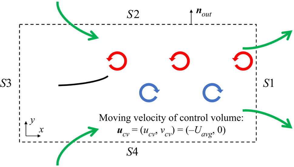
 $F_y^s$ are force components related to the unsteady, pressure, momentum flux and shear stress effects in a CV. Further details are available in the literature (Kurtulus et al. Reference Kurtulus, Scarano and David2007; Jardin et al. Reference Jardin, David and Farcy2009; Shen et al. Reference Shen, Chan and Lin2009). To investigate the effects of the velocity and pressure fields acting on two side-by-side fins in a self-propulsion system, a moving and non-deformable CV around the upper fin is determined close to the fin, similar to that adopted in a recent study of an unconstrained flapping fin by Wu et al. (Reference Wu, Shu, Wan, Wang and Chen2022): xS 1 = Xhead,u + 3, yS 2 = (G 0/2 − Ahead/2) + 0.6, xS 3 = Xhead,u − 0.5 and yS 4 = (G 0/2 − Ahead/2) − 0.6. In the reference frame, CV and CS translate with Uavg along the moving direction; i.e. ucv = (ucv, vcv) = (−Uavg, 0) (figure 5), where Uavg is the average horizontal speed of a fin
 $({U_{avg}} = \int_0^1 {|\partial X/\partial t|\,\textrm{d}s} )$. Here, the lateral spacing of the CV is chosen to cover the flapping range of the upper fin in the CT and MTL modes.
Schematic of the CV around a self-propelled flexible fin. The reference frame of the CV and CS translates with the horizontal speed of the fin (Uavg) toward the negative x-direction. Green arrows indicate induced flows passing through the CSs. During the cycle, the surrounding fluid bleeds into the CV through CSs S2 and S4 (see inward green arrows) and then leaves the CV through CS S1 for propulsion of the fin in the negative x-direction (see outward green arrows).

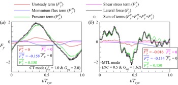
Figure 6 displays the time histories of estimated values for components consisting of the lateral force (Fy) acting on the upper fin at Geq in the CT mode with fa = 1.0 and in the MTL mode with DC = 0.5. As shown, the sum of the unsteady  $(F_y^u)$, momentum flux
 $(F_y^m)$, pressure
 $(F_y^p)$ and shear stress
 $(F_y^s)$ terms in figure 6(a,b) is very similar to the value of Fy, indicating that the lateral force acting on the fin can be decomposed into these four terms. For the upper fin in the CT mode in figure 6(a), the profiles of
 $F_y^m$ and
 $F_y^p$ with the cycle-averaged values of
 $\overline {F_y^m}$ and
 $\overline {F_y^p}$ (see the inset) demonstrate the dominance of the negative value of
 $F_y^m$ and the positive value of
 $F_y^p$ during the cycle, with the balance between the two circulatory lateral force terms, i.e. the momentum flux and pressure terms (
 $\overline {F_y^m}$ and
 $\overline {F_y^p}$), leading to a zero cycle-averaged lateral force
 $(\overline {{F_y}} = 0)$. Similarly, for the MTL mode in figure 6(b), the two circulatory lateral force terms of
 $\overline {F_y^m}$ and
 $\overline {F_y^p}$ are important for achieving an equilibrium state. However, it is evident that a negative unsteady term
 $(\overline {F_y^u} )$ (i.e. added-mass lateral force) contributes to the formation of the lateral equilibrium state for the upper fin. Because this negative unsteady term is a key factor to reduce the equilibrium lateral gap distance between two fins in the MTL mode, the value of Geq for the MTL mode is smaller than that for the CT mode; if the value of
 $\overline {F_y^u}$ is zero for the two fins in the MTL mode, a lateral equilibrium state occurs at G 0,eq = 2.8 (i.e. Geq = 2.6), a value larger than that for the CT mode in figure 3. The contribution of the shear stress term to the generation of the lateral force acting on the upper fin in each mode is negligible. Below (figures 7–10), we present the detailed generation process of each component comprising the lateral force acting on two fins in the CT and MTL modes.
Time histories of estimated values for components comprising the lateral force (Fy) acting on the upper fin at Geq when γ = 1.0: red,  $F_y^u$ (unsteady term); blue,
 $F_y^m$ (momentum flux term); green,
 $F_y^p$ (pressure term); pink,
 $F_y^s$ (shear stress term); black, Fy. For comparison, the sum of the four components in each mode is inserted with circle symbols: (a) CT mode with fa = 1.0 and Geq = 2.0 and (b) MTL mode with DC = 0.5 and Geq = 1.62.

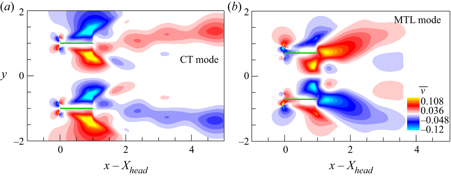
Cycle-averaged lateral velocity contours around two fins at Geq when γ = 1.0: (a) CT mode with fa = 1.0 and (b) MTL mode with DC = 0.5. Green bold lines represent the fins.

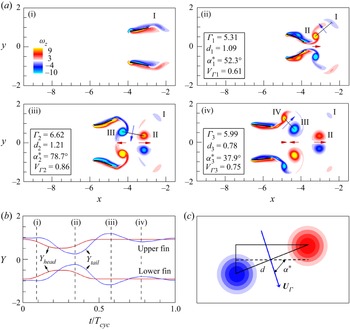
(a) Instantaneous vorticity contours around two fins at Geq in the MTL mode with DC = 0.5 and γ = 1.0. Black bold lines represent the fins. (b) Temporal lateral positions of the leading edge (Yhead) (red) and trailing edge (Ytail) (blue) for two fins. (c) Schematic of two consecutive vortices to explain the vortex-induced velocity ( $\textbf{U}_{\varGamma}$) based on the vortex dipole model. Four instances (i–iv) in (a) are chosen based on the local maximum and minimum Ytail in (b). The four vortices behind the upper fin in (a) are denoted by I, II, III and IV based on the sequence of vortex shedding (from I to IV), and the induced velocities between vortices I and II at instance (ii), between vortices II and III at instance (iii) and between vortices III and IV at instance (iv) are denoted by the blue arrows. In (a), the induced horizontal velocities between the upper and lower fins are denoted by the red arrows. The lengths of the blue and red arrows are proportional to the strengths of the induced velocities.

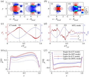
(a,b) Instantaneous pressure contours around two fins at Geq with γ = 1.0 when the lateral force (Fy) acting on the upper fin reaches its (i) maximum and (ii) minimum: (a) CT mode with fa = 1.0 and (b) MTL mode with DC = 0.5. In (a,b), green bold lines represent the fins. (c,d) Temporal variations of the lateral force (Fy) (red) and the average lateral velocity (Vavg) (blue) for each case. (e,f) Conditionally averaged (e) positive pressure  $(\overline {{p^{pos}}} )$ and (f) negative pressure
 $(\overline {{p^{neg}}} )$ along the lower surface of the upper fin at Geq: red circle, CT mode with fa = 1.0; blue triangle, MTL mode with DC = 0.5. For comparison, data for an isolated fin in the CT mode with fa = 1.0 (red dashed line) and MT mode (coasting at the maximum Yhead) with DC = 0.5 (blue dashed line) are included.

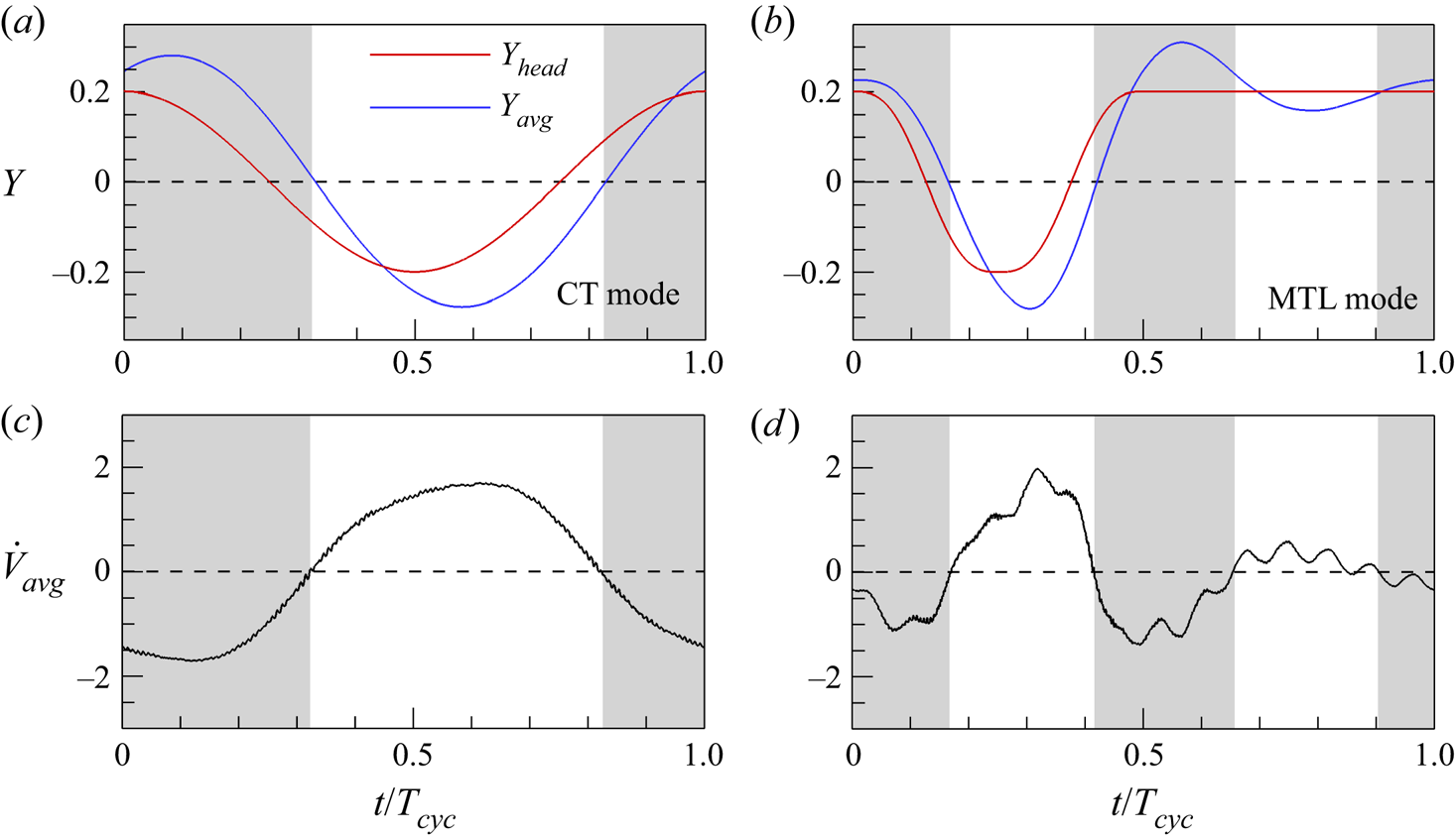
Time histories of (a,b) the lateral position of the leading edge (Yhead) and the average lateral position (Yavg) and (c,d) the average lateral acceleration  $({\dot{V}_{avg}})$ for the upper fin at Geq when γ = 1.0: (a,c) CT mode with fa = 1.0 and (b,d) MTL mode with DC = 0.5. White and grey regions in each figure indicate acceleration states toward upward
 $({\dot{V}_{avg}} > 0)$ and downward
 $({\dot{V}_{avg}} < 0)$ directions, respectively. Horizontal dashed line indicates a zero value.

To examine why the negative cycle-averaged momentum flux term  $(\overline {F_y^m} )$ occurs for the two fins in the CT and MTL modes, the cycle-averaged lateral velocity contours around two fins at Geq are presented in figure 7. The contours behind the upper fin in the CT and MTL modes show the dominance of the positive cycle-averaged lateral velocity (red contour). Because a positive horizontal velocity (u) behind a fin is expected to occur to propel toward the negative x-direction, an upward deflected jet with the dominance of a positive lateral velocity behind a fin during the cycle acts to induce a negative
 $\overline {F_y^m}$ (see the momentum flux term at the CS S1 in (3.3)). It should be noted that because the momentum flux term in the y-direction is coupled with the horizontal velocity (3.3), the jet strength shown in figure 7 is not directly proportional to the magnitude of
 $\overline {F_y^m}$.
Figure 8 shows the instantaneous vorticity contours around two fins at Geq for the MTL mode with DC = 0.5 to explain the formation process of the cycle-averaged lateral velocity for intermittent swimming (figure 7b). Four instances (i‒iv) in figure 8(a) are selected based on the local maximum and minimum Ytail (see figure 8b). In figure 8(a), four vortices (I‒IV) are generated by the upper fin over each cycle period, and they induce local lateral velocities (see the blue arrows), i.e. positive lateral velocities by vortex pairs (I, II) and (III, IV) and negative lateral velocity by a vortex pair (II, III). The horizontal flows between the counter-rotating vortices generated by the upper and lower fins (see the red arrows) lead to the downstream advection of vortices II and IV and the upstream advection of vortex III, resulting in an increase (decrease) of the positive (negative) lateral velocities. For a comparison between the vortex-induced positive and negative lateral velocities in terms of the magnitude, the vortex dipole model proposed by Godoy-Diana et al. (Reference Godoy-Diana, Marais, Aider and Wesfreid2009) is employed. Based on the vortex dipole model (figure 8c), the vortex-induced horizontal ( $U_{\varGamma}$) and lateral (
 $V_{\varGamma}$) velocities can be approximated as
 ${\boldsymbol{U}_\varGamma } = ({U_\varGamma },{V_\varGamma }) = ((\varGamma /2{\rm \pi} d)\cos {\alpha ^\ast },(\varGamma /2{\rm \pi} d)\sin {\alpha ^\ast })$, where
 ${\boldsymbol{U}_\varGamma } = \boldsymbol{U}_\varGamma ^\ast{/}U_{ref}^\ast $,
 $\varGamma = {\varGamma ^\ast }/(U_{ref}^\ast {L^\ast })$,
 $d = {d^\ast }/{L^\ast }$ and α* are correspondingly the induced velocity, the average circulation of two vortices in the dipole, the distance between the vortex cores, and the orientation angle of
 $\textbf{U}_{\varGamma}$ relative to the x-direction (Godoy-Diana et al. Reference Godoy-Diana, Marais, Aider and Wesfreid2009; Zheng & Wei Reference Zheng and Wei2012; Kim & Lee Reference Kim and Lee2019). Each value of
 ${\varGamma}$, d and α* is estimated when an upstream vortex in a dipole is shed from the trailing edge of the fin. The vortex circulation is calculated through the integration of the vorticity over a rectangular area, and the integration area is determined by performing Gaussian fits
 $({\textrm{e}^{( - x_i^2/\sigma _i^2)}})$ along the x- and y-directions based on the positions of the vorticity maximum and minimum. The size of each vortex along the x- and y-directions is defined as 2σi (Godoy-Diana et al. Reference Godoy-Diana, Marais, Aider and Wesfreid2009; Zheng & Wei Reference Zheng and Wei2012). For dipole (I, II) at instance (ii), dipole (II, III) at instance (iii) and dipole (III, IV) at instance (iv) in figure 8(a), the estimated values of
 ${\varGamma_{j}}$, dj,
 $\alpha _j^\ast $ and
 $V_{\varGamma j}$, respectively, are listed in the inset, where the subscript j represents a value formed between the jth vortex and the j + 1th vortex (for example, d 1 is the distance between vortices I and II). A comparison between the vortex-induced positive and negative lateral velocities (see the insets in figure 8a) demonstrates that the presence of the positive cycle-averaged lateral velocity behind the upper fin in the MTL mode in figure 7(b) is closely associated with the large contribution of the positive
 $V_{\varGamma}$1 and
 $V_{\varGamma}$3 compared with that of the negative
 $V_{\varGamma}$2.
The overall process for the creation of vortices and their induction of local lateral velocities for the upper fin in the MTL mode is similar to previous findings pertaining to two side-by-side anti-phase flapping rigid/flexible fins (Dewey et al. Reference Dewey, Quinn, Boschitsch and Smits2014; Peng et al. Reference Peng, Huang and Lu2018) and for a single rigid/flexible fin near the ground (Quinn et al. Reference Quinn, Moored, Dewey and Smits2014; Dai et al. Reference Dai, He and Zhang2016; Park et al. Reference Park, Kim and Sung2017; Kurt et al. Reference Kurt, Cochran-Carney, Zhong, Mivehchi, Quinn and Moored2019) during continuous swimming. Furthermore, the role of the induced horizontal flows on the increase (decrease) of the positive (negative) lateral velocities between vortices for the upper fin in the MTL mode is similar to our observation from the CT mode (not shown here for brevity). Nonetheless, a careful inspection of the vortex patterns in figure 7 shows less coherence of the vortex organization behind the upper fin in the MTL mode than that in the CT mode due to the presence of a coasting period in the MTL mode. Furthermore, the strength of the lateral jet deflection is greater in the MTL mode than in the CT mode in figure 7 due to a large difference between the vortex-induced positive and negative lateral velocities right behind the upper fin during the cycle. Temporal evolutions of the vortex structures for the generation of an upward deflection jet behind the upper fin in the MTL mode in figure 8(a) are found for all DC (0.1 ≤ DC < 1.0), consistent with a previous experimental study of a single pitching fin under intermittent swimming (MT mode) (Floryan, Buren & Smits Reference Floryan, Buren and Smits2017). However, the properties of vortex structures (i.e.  ${\varGamma}$, d and α*) and their advection speeds vary according to the intermittency (i.e. DC).
Next, in order to explain the generation of the positive cycle-averaged pressure term  $(\overline {F_y^p} )$ for the upper fin in the CT and MTL modes in figure 6, the instantaneous pressure contours around two fins at Geq are presented in figure 9(a,b). Figure 9(c,d) show the temporal variations of the lateral force (Fy) (red) and the average lateral velocity (Vavg) (blue) for the upper fin, where the average lateral velocity (Vavg) along a fin is defined as
 ${V_{avg}} = \int_0^1 {(\partial Y(s,t)/\partial t)\,\textrm{d}s}$. The pressure contours in each mode are extracted when the lateral force (Fy) acting on the upper fin reaches its maximum (figure 9a-i,b-i) and minimum (figure 9a-ii,b-ii) (see the vertical dashed lines in figure 9c,d). Consistent with previous findings for two side-by-side flexible fins during continuous swimming (Peng et al. Reference Peng, Huang and Lu2018), the positive (figure 9a-i,b-i) and negative pressures (figure 9a-ii,b-ii) around two fins are enhanced by sharing the pressure field for all modes during the inward and outward motions, respectively (figure 9c,d). The enhancement of the pressures around two side-by-side fins by schooling can be estimated through a comparison with those around a single fin in each mode (i.e. CT mode and MT mode coasting at the maximum Yhead; see only the red line in figure 2a,d). To quantify the enhancement of each component of the positive and negative pressure, conditional averaging of the positive and negative pressure during the cycle is performed; these results (
 $\overline {{p^{pos}}}$ and
 $\overline {{p^{neg}}}$) are plotted in figure 9(e,f). Here,
 $\overline {{p^{pos}}}$ and
 $\overline {{p^{neg}}}$ are the conditionally averaged positive and negative pressure along the under surface of the upper (single) fin, respectively, during the cycle. A comparison of the conditionally averaged pressure between the upper fin and single fin shows that the increasing magnitude of the positive pressure by schooling in each mode exceeds that of the negative component, leading to a positive
 $\overline {F_y^p}$ for the upper fin in the CT and MTL modes in figure 6. The dominance of the enhanced positive pressure for the upper fin in the CT and MTL modes in figure 9 is consistent with a previous observation, commonly known as the ‘cushion effect’, which serves to lift an actively flapping rigid/flexible body and a stationary body near the ground (Zhang et al. Reference Zhang, Huang and Lu2017; Kurt et al. Reference Kurt, Cochran-Carney, Zhong, Mivehchi, Quinn and Moored2019; Jeong et al. Reference Jeong, Lee and Park2021). On the other hand, the increase of
 $\overline {{p^{pos}}}$ for the upper fin in the MTL mode relative to a single fin in the MT mode (see the blue colouring in figure 9e) is larger than that in the CT mode due to the small value of Geq, suggesting a large difference of the values of
 $\overline {F_y^p}$ between the single and upper fins in the MT/MTL mode compared with that in the CT mode (
 $\Delta \overline {F_y^p} = 0.158$ for the CT mode and 0.168 for the MT/MTL mode).
Finally, to analyse how the negative cycle-averaged unsteady term  $(\overline {F_y^u} )$ in figure 6 arises for intermittent swimming (MTL mode), the time histories of the lateral position of the leading edge (Yhead), the average lateral position
 $({Y_{avg}} = \int_0^1 {Y(s,t)\,\textrm{d}s} )$ and the average lateral acceleration
 $({\dot{V}_{avg}} = \textrm{d}{V_{avg}}/\textrm{d}t)$ of the upper fin at Geq during the cycle are presented in figure 10. Here, the lateral position of Yhead and Yavg for the upper fin in the CT and MTL modes is modulated by subtracting G 0,eq/2 − Ahead/2. For the upper fin in the CT mode, the average lateral position (Yavg) in figure 10(a) shows a symmetric profile during the cycle (consistent with the variation of Ytail in figure 4a), and thus the balanced variation of
 ${\dot{V}_{avg}}$ between positive and negative values during the cycle in figure 10(c) results in the zero
 $\overline {F_y^u}$ shown in figure 6. Contrary to the observation in the CT mode, the profiles of Yavg and
 ${\dot{V}_{avg}}$ for the MTL mode are complicated with asymmetric motions during the cycle in figure 10(b,d) (also see figure 4c). The signs of
 ${\dot{V}_{avg}}$ are negative (grey regions) and positive (white regions) when the lateral positions of Yavg for the upper fin are above and below the equilibrium positions (Y = 0 during the burst period (0 ≤ t/Tcyc < 0.5) and Y = 0.2 during the coast period (0.5 ≤ t/Tcyc < 1.0)). This relationship between Yavg and
 ${\dot{V}_{avg}}$ can be explained by a restoring force acting in the direction of the equilibrium positions under the prescribed bursting or coasting motion. Interestingly, the magnitude of the positive
 ${\dot{V}_{avg}}$ is larger than that of the negative
 ${\dot{V}_{avg}}$ during the burst period because the large lateral displacement of Yavg near t/Tcyc = 0.3 (from the equilibrium position) due to the elastic response by the passive flexibility generates a strong restoring force acting in the upward direction. This result indicates that the negative value of
 $\overline {F_y^u}$ for the upper fin in the MTL mode in figure 6 is attributable to the positive lateral fin (or flow) accelerations (see the unsteady term in (3.3)) caused by the strong restoring force. During the coast period, the values of
 ${\dot{V}_{avg}}$ are relatively small due to the weakened restoring force as the lateral spacing between Yavg and the equilibrium position (Y = 0.2) is reduced. To support our observation in figure 10, the root-mean-square of the conditional lateral accelerations (
 ${(\dot{V}_{avg}^{pos})_{rms}}$ and
 ${(\dot{V}_{avg}^{neg})_{rms}}$) during the cycle is calculated, where
 $\dot{V}_{avg}^{pos}$ and
 $\dot{V}_{avg}^{neg}$ are the positive and negative components of the lateral accelerations of a fin, respectively. The estimated value of
 ${(\dot{V}_{avg}^{pos})_{rms}}$ for the upper fin in the MTL mode (=0.637) is found to be larger than that of
 ${(\dot{V}_{avg}^{neg})_{rms}}$ (=0.564), indicating the dominance of the positive lateral fin acceleration for intermittent swimming.
The hydrodynamic mechanism leading to lateral equilibrium states of fin(s) for continuous swimming was examined in an experimental study of a single pitching rigid fin near the ground in a tethered system (Kurt et al. Reference Kurt, Cochran-Carney, Zhong, Mivehchi, Quinn and Moored2019). Kurt et al. (Reference Kurt, Cochran-Carney, Zhong, Mivehchi, Quinn and Moored2019) found that a stable equilibrium lateral position of a pitching rigid fin on the ground is mainly determined by the balance between the enhanced positive pressures and jet deflections; moreover, the contribution of the negative cycle-averaged added-mass lateral force on the equilibrium state is small. Despite the different model set-ups (e.g. self-propulsion, passive flexibility and heaving motion), the underlying mechanism leading to an equilibrium state for two side-by-side flexible fins in the CT mode (figures 7, 9 and 10) is similar to that for a single rigid fin near the ground as found by Kurt et al. (Reference Kurt, Cochran-Carney, Zhong, Mivehchi, Quinn and Moored2019). Together with previous observations using two side-by-side anti-phase flapping rigid/flexible fins in tethered (Dewey et al. Reference Dewey, Quinn, Boschitsch and Smits2014) and self-propulsion systems (Peng et al. Reference Peng, Huang and Lu2018; Lin et al. Reference Lin, Wu, Zhang and Yang2021) and a single rigid/flexible fin in fixed (Quinn et al. Reference Quinn, Moored, Dewey and Smits2014; Zhong et al. Reference Zhong, Han, Moored and Quinn2021) and free-swimming conditions (Dai et al. Reference Dai, He and Zhang2016; Park et al. Reference Park, Kim and Sung2017; Zhang et al. Reference Zhang, Huang and Lu2017) under continuous heaving or pitching motions, the implication of the present findings is that the circulatory lateral forces caused by the enhanced positive pressures and jet deflections play a dominant role in determining the lateral equilibrium state of fin(s) in continuous (symmetric) swimming regardless of the model set-up.
In contrast, for the MTL mode, the relationship between the lateral position Yavg and the acceleration  ${\dot{V}_{avg}}$ in figure 10(b,d) indicates that the asymmetric flapping kinematics of the average lateral motion during the cycle is important in the generation of the added-mass lateral force. However, it should be noted that for two side-by-side rigid fins in the MTL mode with no passive flexibility (Yavg = Yhead), the lateral equilibrium state of the two fins is not influenced by the added-mass force because the restoring forces acting in the downward and upward directions during the burst period are balanced due to the symmetric profile of Yavg with respect to the equilibrium position of Y = 0 (see the red line in figure 10b), and the restoring force during the coast period is zero. These results suggest that the asymmetry of the body response by the passive flexibility with respect to the equilibrium positions of the bursting and coasting motions is crucial in determining the distinct physical mechanism in the MTL mode.
Consistent with the observation for the CT mode, the HT mode shows that only circulatory lateral forces without any added-mass lateral force (i.e. zero  $\overline {F_y^u}$) influence the equilibrium lateral gap distance between two flexible fins (not shown here) due to the symmetric nature of the body response (figure 4b). Similarly, two rigid fins in the HT mode (Yhead = Yavg) maintain a lateral stable state due to the balance between the circulatory lateral forces. The current observations from the CT, HT and MTL modes demonstrate that when the lateral motion of two fins is symmetric with respect to an equilibrium position regardless of flexibility and/or intermittency, a lateral equilibrium state is determined by the circulatory lateral forces caused by the enhanced positive pressures and jet deflections. Because we consider only continuous swimming with the symmetric kinematics, the asymmetric kinematics of a continuously swimming fin with respect to the equilibrium position, e.g. prescribed lateral motion with different periods of upstroke and downstroke (Zhao et al. Reference Zhao, Mao, Pan, Huang and Sung2021), most likely leads to the generation of the added-mass lateral force.
3.2. Schooling performance of continuous and intermittent swimmers in a stable equilibrium state
In this section, the schooling performances of two fins in the CT and MTL modes in a stable equilibrium state are investigated when the cruising speed and input power are varied by changing the adjustable frequency ratio (fa) for continuous swimming and the DC for intermittent swimming. This allows for an understanding of the performance enhancement achieved by simultaneously utilizing schooling behaviour and intermittent swimming.
The COT has been suggested to compare the propulsive performance between continuous and intermittent swimmers (Chung Reference Chung2009; Akoz & Moored Reference Akoz and Moored2018; Dai et al. Reference Dai, He, Zhang and Zhang2018a; Akoz et al. Reference Akoz, Han, Liu, Dong and Moored2019; Liu et al. Reference Liu, Huang and Lu2020). The COT (or the power-to-speed ratio), which is the energy required to travel a unit distance during one cycle period, is defined as follows (Park & Sung Reference Park and Sung2016):
 \begin{equation}COT = \overline {{P_{avg}}} /\overline {{U_{avg}}} .\end{equation}
Because the structure-to-fluid mass ratio is fixed in our simulation (i.e. ρ = 1.0), the inertial effect on the COT is not considered (Park & Sung Reference Park and Sung2016). The cycle-averaged horizontal speed (or cruising speed)  $(\overline {{U_{avg}}} )$ and the cycle-averaged input power
 $(\overline {{P_{avg}}} )$ of a fin are defined as
 \begin{gather}\overline {{U_{avg}}} = \frac{1}{{{T_{cyc}}}}\int_0^{{T_{cyc}}} {{U_{avg}}\,\textrm{d}t} ,\end{gather}
 \begin{gather}\overline {{P_{avg}}} = \frac{1}{{{T_{cyc}}}}\int_0^{{T_{cyc}}} {{P_{avg}}} \,\textrm{d}t = \frac{1}{{{T_{cyc}}}}\int_0^{{T_{cyc}}} {a(t)\left( {\int_0^1 {{\boldsymbol{F}_L}\boldsymbol{\cdot }\frac{{\partial \boldsymbol{X}}}{{\partial t}}\textrm{d}s} } \right)} \,\textrm{d}t,\end{gather}
where the average input power along a fin (Pavg) is defined as  ${P_{avg}} = a(t)\int_0^1 {\boldsymbol{F}_L}\boldsymbol{\cdot } (\partial \boldsymbol{X}/\partial t)\,\textrm{d}s$. In (3.6), the shielding function a(t) is used to consider only the work during the burst phase of intermittent swimming (Dai et al. Reference Dai, He, Zhang and Zhang2018a; Liu et al. Reference Liu, Huang and Lu2020)
 \begin{equation}a(t) = \left\{ {\begin{array}{{@{}ll}} 0&{\textrm{if}\ DC \ne 1.0\ \& \ t \in \textrm{coast}\ \textrm{period,}}\\ 1&{\textrm{otherwise}.} \end{array}} \right.\end{equation}
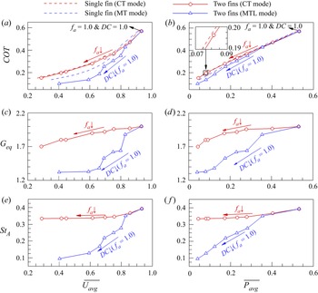
Figure 11(a,b) show the variation of the COT for two fins in the CT and MTL modes at Geq as a function of  $\overline {{U_{avg}}}$ and as a function of
 $\overline {{P_{avg}}}$ respectively. Here, the values of fa for the CT mode and DC for the MTL mode are varied in the range of 0.5 ≤ fa ≤ 1.0 and 0.1 ≤ DC ≤ 1.0, respectively. For comparison, values for a single fin in the CT and MT modes are also included. For two parallel swimming fins in the CT and MTL modes, symmetric motion of the upper and lower fins requires the same cycle-averaged input power (i.e.
 $\overline {{P_{avg}}} = \overline {{P_{avg,u}}} = \overline {{P_{avg,l}}}$), and the cruising speed of the upper fin is always identical to that of the lower fin (i.e.
 $\overline {{U_{avg}}} = \overline {{U_{avg,u}}} = \overline {{U_{avg,l}}}$); thus, COT = COTu = COTl. The COT values for two fins in the CT and MTL modes (red and blue symbols) decrease with a reduction of fa and DC, respectively, similar to the variation for a single fin in the CT and MT modes (dashed lines). The magnitudes of the COT for a single fin in the MT mode are smaller than those for the CT mode at the same
 $\overline {{U_{avg}}}$ or
 $\overline {{P_{avg}}}$, consistent with previous findings for a single self-propelled flexible fin during intermittent swimming (Dai et al. Reference Dai, He, Zhang and Zhang2018a; Liu et al. Reference Liu, Huang and Lu2020), suggesting the presence of a benefit from an intermittent swimming gait. Furthermore, the magnitudes of the COT for two fins in the MTL mode are smaller than those of a single fin in the MT mode when the values of
 $\overline {{U_{avg}}}$ (figure 11a) or
 $\overline {{P_{avg}}}$ (figure 11b) are identical, indicating the presence of an additional benefit from schooling behaviours due to the influence of shared pressures between two side-by-side flexible fins (e.g. see figure 9) (Peng et al. Reference Peng, Huang and Lu2018). These observations indicate that when two side-by-side flexible fins utilize the MTL mode, the fins can reduce the value of COT significantly by realizing not only a benefit from an intermittent swimming gait but also a schooling benefit. In addition, a large reduction of the COT for two fins relative to a single fin for the MTL/MT mode compared with that for the CT mode in figure 11(a,b) suggests the enhanced schooling benefit. As shown in figure 11(c,d), the enhanced schooling benefit for two fins in the MTL mode compared with that in the CT mode is related to the smaller magnitudes of Geq in the MTL mode when the values of
 $\overline {{U_{avg}}}$ or
 $\overline {{P_{avg}}}$ are identical (also see figure 3). Because the pressure difference between the above and under surfaces of two side-by-side flexible fins during inward and outward motions increases as the lateral spacing between them decreases (Peng et al. Reference Peng, Huang and Lu2018), the large pressure differences across the fins caused by the small Geq for two fins in the MTL mode (figure 11c,d) result in a significant enhancement of the thrust force (or propulsive performance). However, it should be noted that the passive deflection with a decreased flapping amplitude stemming from a small lateral gap distance in the MTL mode (not shown) has a role in reducing the thrust force/performance in this case (Park et al. Reference Park, Kim and Sung2017). In figure 11(e,f), the decrease of Geq with respect to a decrease of fa in the CT mode and DC in the MTL mode is associated with a reduction of the Strouhal number (StA), similar to previous observations for a pitching rigid fin near the ground (Kurt et al. Reference Kurt, Cochran-Carney, Zhong, Mivehchi, Quinn and Moored2019; Zhong et al. Reference Zhong, Han, Moored and Quinn2021). Here, the Strouhal number (StA), which is an important factor to describe the kinematics of swimming motion, is defined as
 $S{t_A} = {A_{tail}}/(\overline {{U_{avg}}} {T_{cyc}})$ (Dai et al. Reference Dai, He, Zhang and Zhang2018a), where Atail is the peak-to-peak amplitude of the trailing edge.
Variations of the (a,b) COT, (c,d) equilibrium lateral gap distance between two fins (Geq) and (e,f) the Strouhal number based on the peak-to-peak tail amplitude (StA) (a,c,e) as a function of the cruising speed  $(\overline {{U_{avg}}} )$ and (b,d,f) as a function of the cycle-averaged input power
 $(\overline {{P_{avg}}} )$ for two fins with γ = 1.0 in the CT mode in the range of 0.5 ≤ fa ≤ 1.0 (red circle) and in the MTL mode in the range of 0.1 ≤ DC ≤ 1.0 (blue triangle). In (a,b), red and blue dashed lines indicate values for a single fin in the CT and MT modes, respectively.

3.3. Passive flexibility effects
It is known that the role of passive flexibility is important in determining the propulsive performance and wake properties of self-propelled flexible fin(s) during continuous swimming (Hua, Zhu & Lu Reference Hua, Zhu and Lu2013; Zhu et al. Reference Zhu, He and Zhang2014a,Reference Zhu, He and Zhangb; Peng et al. Reference Peng, Huang and Lu2018; Jeong et al. Reference Jeong, Lee and Park2021). Despite many studies of the role of passive flexibility for self-propelled flexible fin(s) under continuous swimming, the effects of flexibility on the propulsive performance and wake structures of self-propelled fin(s) with an intermittent swimming style are not fully understood. In this section, the influence of the passive flexibility on the COT and wake structures of two stable fins in the CT and MTL modes at Geq is examined in a wide range of 0.3 ≤ γ ≤ ∞ to show the importance of passive flexibility by identifying its distinctive role during continuous and intermittent swimming.
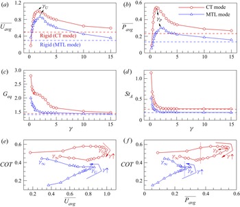
Figures 12(a) and 12(d) show the variations of the cruising speed  $(\overline {{U_{avg}}} )$, cycle-averaged input power
 $(\overline {{P_{avg}}} )$, equilibrium lateral gap distance (Geq) and the Strouhal number (StA) as a function of the bending rigidity (γ) for two fins in the CT mode with fa = 1.0 and in the MTL mode with DC = 0.5. In figure 12(a,b), the values of
 $\overline {{U_{avg}}}$ and
 $\overline {{P_{avg}}}$ for the CT and MTL modes increase with an increase of γ and reach the corresponding maximum values (see γU and γP, where γU and γP indicate the critical bending rigidities for the maximum
 $\overline {{U_{avg}}}$ and
 $\overline {{P_{avg}}}$). As the value of γ increases further, the values of
 $\overline {{U_{avg}}}$ and
 $\overline {{P_{avg}}}$ decrease toward those for rigid cases (see the horizontal dashed lines in figure 12a,b), similar to previous observations of self-propelled flexible fin(s) during continuous swimming (Hua et al. Reference Hua, Zhu and Lu2013; Peng et al. Reference Peng, Huang and Lu2018; Jeong et al. Reference Jeong, Lee and Park2021). In this case, the values of
 $\overline {{U_{avg}}}$ and
 $\overline {{P_{avg}}}$ are estimated when the two fins have equilibrium lateral gap distances, as shown in figure 12(c). The decreasing trend of Geq for the CT and MTL modes with an increase of γ stems from the reduction of StA (figure 12d), consistent with our observation in figure 11. In figure 12(e,f), the most interesting observation is that the COT for the CT mode (red circle) can be reduced when γ > γU (or γP) while maintaining an identical
 $\overline {{U_{avg}}}$ (or
 $\overline {{P_{avg}}}$), whereas in the MTL mode (blue triangle), adopting a low γ (γ < γU or γ < γP) leads to a reduced COT of the two fins. This finding suggests that the beneficial schooling performance of two self-propelled flexible fins during continuous and intermittent swimming can be achieved by adjusting the flexibility in a desired propulsion state (i.e. maintaining an identical
 $\overline {{U_{avg}}}$ (or
 $\overline {{P_{avg}}}$)). Although the value of DC for the MTL mode is set to 0.5 in figure 12, the profile of the COT shifts toward the lower left as the value of DC decreases (see the trend of COT at a fixed γ = 1.0 in figure 11).
(a–d) Variations of the (a) cruising speed  $(\overline {{U_{avg}}} )$, (b) cycle-averaged input power
 $(\overline {{P_{avg}}} )$, (c) equilibrium lateral gap distance (Geq) and (d) the Strouhal number based on the peak-to-peak tail amplitude (StA) as a function of the bending rigidity (γ) for two flexible fins in the CT mode with fa = 1.0 (red circle) and in the MTL mode with DC = 0.5 (blue triangle). In (a–d), red and blue horizontal dashed lines indicate the corresponding values for two rigid fins in the CT mode and MTL mode, respectively. (e,f) Variations of the COT (e) as a function of
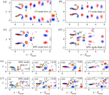
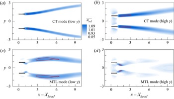
 $\overline {{U_{avg}}}$ and (f) as a function of
 $\overline {{P_{avg}}}$ for two fins in each mode in the wide range of 0.3 ≤ γ ≤ ∞.

In an effort to explain the opposite trend due to a change in the passive flexibility in the two distinct swimming styles, the instantaneous vorticity contours around two fins at Geq with low and high values of γ in the CT mode (γ = 0.6 and 4.0) and in the MTL mode (γ = 1.5 and 5.0) are presented in figure 13 when the values of  $\overline {{P_{avg}}}$ for each mode are identical (see red and blue vertical lines in figure 12f). For the CT mode in figure 13(a,b), the vortex structures for both low and high γ values are deflected away from the centreline; i.e. this reflects the dominance of the positive lateral velocity induced by vortex pair (II, III) compared with the negative lateral velocity induced by vortex pair (I, II). However, the lateral advection of vortices is shown to be dominant for a low γ compared with that for a high γ because the stronger vortices for the low γ (
 ${\varGamma}$1 = 6.32 and
 ${\varGamma}$2 = 6.25 for the low γ and
 ${\varGamma}$1 = 5.87 and
 ${\varGamma}$2 = 5.52 for the high γ) tend to destabilize the wake with regard to symmetry preservation (Zheng & Wei Reference Zheng and Wei2012; Zhu et al. Reference Zhu, He and Zhang2014b).
(a–d) Instantaneous vorticity contours around two fins at Geq in (a,b) the CT mode with fa = 1.0 and (c,d) the MTL mode with DC = 0.5: (a) γ = 0.6, (b) γ = 4.0, (c) γ = 1.5 and (d) γ = 5.0. Black bold lines represent the fins. In each mode, the values of the cycle-averaged input power  $(\overline {{P_{avg}}} )$ for two fins with a low and high γ value are identical. (e,f) Time-evolving vorticity contours around the upper fin in the MTL mode with (e) low γ (=1.5) and (f) high γ (=5.0) values. In (e,f), green arrows indicate vortex-induced velocities with a positive horizontal component. The lengths of the green arrows are proportional to the strengths of the induced velocities.

To extract the thrust component of a momentum jet in the wake further, the contours of the cycle-averaged relative horizontal velocity  $(\overline {{u_{rel}}} )$ behind two fins are analysed in figure 14. The value of
 $\overline {{u_{rel}}}$ is calculated by subtracting
 $\overline {{u^{neg}}}$ from
 $\overline u$ to take into account the moving effects of the fins in a self-propulsion system (Peng et al. Reference Peng, Huang and Lu2018; Wu et al. Reference Wu, Shu, Wan, Wang and Chen2022), as self-propelled fins propel toward the negative x-direction with a negatively induced horizontal flow around the fins (Park & Sung Reference Park and Sung2016; Park et al. Reference Park, Kim and Sung2017; Jeong et al. Reference Jeong, Lee and Park2021; Wu et al. Reference Wu, Shu, Wan, Wang and Chen2022). Here,
 $\overline {{u^{neg}}}$ is the conditionally averaged negative horizontal flow velocity around a fin. Because the larger inclination angle of the jet velocity for the CT mode with a low γ acts to decrease the thrust force due to the excessive waste of the backward momentum of the fluid into the y-direction, the strong jet velocity (see red solid lines in figure 14a,b) stemming from the smaller jet inclination angle for the CT mode with the high γ is beneficial for propulsion (Dong, Mittal & Najjar Reference Dong, Mittal and Najjar2006; Zhu et al. Reference Zhu, He and Zhang2014b; Peng et al. Reference Peng, Huang and Lu2018), i.e. a small COT in figure 12.
Cycle-averaged relative horizontal velocity  $(\overline {{u_{rel}}} )$ behind two fins at Geq for (a,b) the CT mode with fa = 1.0 and (c,d) the MTL mode with DC = 0.5: (a) γ = 0.6, (b) γ = 4.0, (c) γ = 1.5 and (d) γ = 5.0. Black bold lines represent the fins. Red solid lines in (a,b) and (c,d) indicate contour levels of
 $\overline {{u_{rel}}} = 1.15$ and 1.0, respectively.

For the MTL mode, the wake structures with a low γ (=1.5) in figure 13(c) are similar to those when γ = 1.0 in figure 8. However, for a high γ ( = 5.0), both vortices III and IV consist of two components, i.e. (III′ and III′′) and (IV′ and IV′′), as the trailing edge vortex (TEV) (III′ and IV′) is shed alone from the upper fin with a high γ before an identically signed leading edge vortex (LEV) (III′′ and IV′′) generated by the previous motion reaches the trailing edge, after which the LEV is also solely shed (Lua et al. Reference Lua, Lim, Yeo and Oo2007). It should be noted that vortices I~III (figure 13a,b) and III~IV (figure 13c) are formed by constructive merging between the LEV and TEV. This separation of the LEV and TEV occurs due to the slow advection speed of the LEV caused by the high γ with a small  $S{t_c}( = f_f^\ast {L^\ast }/U_{ref}^\ast = {L^\ast }/(T_{cyc}^\ast U_{ref}^\ast ))$ (in this case, Stc = 0.26), similar to a previous experimental observation for a continuous heaving rigid fin in a tethered system (Lewin & Haj-Hariri Reference Lewin and Haj-Hariri2003; Lua et al. Reference Lua, Lim, Yeo and Oo2007). It is also noted that for the CT mode with a high γ, the value of Stc is relatively large (Stc = 0.48), resulting in merging between the vortices. When the value of γ is high, the reduction of the value of Stc occurs more readily during intermittent swimming compared with continuous swimming because the coasting behaviour during intermittent swimming increases the total cycle period (Dai et al. Reference Dai, He, Zhang and Zhang2018a). For the MTL mode with the low γ in figure 13(c), the merged vortices III and IV form behind the upper fin regardless of the value of Stc because the delayed lateral motion of the trailing edge relative to the leading edge stemming from the large passive flexibility helps to ensure time for the LEV to merge with the TEV. Similarly, the postponed response of the trailing edge relative to the leading edge for the CT mode with a low γ leads to the merged vortices shown in figure 13(a) regardless of the value of Stc.
Because the wake structures behind the two fins in the MTL mode with the low and high γ generate unique jet velocity patterns, as shown in figure 14(c,d), the time-evolving vorticity contours around the upper fin for the MTL mode are analysed in figure 13(e,f). In figure 13(e) with a low γ, a positive horizontal flow is induced by the interaction between positive and negative vortices IV and III (see the green arrows at instances (ii), (iii) and (iv)). As the vortex pair advects in a downstream region, the mutual induction between them generates an organized long jet velocity, as shown in figure 14(c). The jet structure curved outward with respect to the centreline is due to the rotation of positive vortex IV in a clockwise manner with respect to the strong negative vortex III by a discrepancy in the vortex strength (Quinn et al. Reference Quinn, Moored, Dewey and Smits2014). On the other hand, for a high γ, positive and negative vortices II and III′ (figure 13f–i) are important to generate a local jet structure immediately behind the upper fin, as depicted in figure 14(d). However, as shown in figures 13(f-ii), 13(f-iii) and 13(f-iv), the horizontal component of the induced flow between vortices II and III′ disappears, and the positive flows induced by vortex pairs (III′, IV′), (IV′, V) and (III′, IV′′) are relatively weak, leading to the locally organized jet velocity with weak strength shown in figure 14(d) (i.e. a large COT compared with that with the low γ in figure 12).
4. Summary and conclusion
The lateral stability and schooling performance of two self-propelled anti-phase flapping flexible fins in a side-by-side configuration for intermittent swimming (with laterally constrained heaving motions) were investigated numerically in comparison with those for continuous swimming. Although three types of intermittent swimming modes for two side-by-side fins (HT, MTS and MTL modes) were considered, only the fins in the MTL and HT modes achieved lateral equilibrium states, demonstrating that two side-by-side flexible fins in a proper form of intermittent swimming motion can maintain a lateral equilibrium state. Based on a CV analysis, it was shown that the lateral equilibrium states of the upper fin in the MTL mode are influenced by not only the circulatory lateral forces but also by the added-mass lateral force, causing the equilibrium lateral gap distance to be smaller than that in the CT mode. The presence of the negative added-mass lateral force for the upper fin in the MTL mode was attributed to the asymmetric flapping kinematics caused by passive flexibility with respect to equilibrium positions of the bursting and coasting motions. When the flapping kinematics of two flexible/rigid fins was symmetric in the CT, HT and MTL modes, only the circulatory lateral forces were important in determining the equilibrium lateral gap distance, indicating that the symmetry of the flapping kinematics is the key factor generating the added-mass lateral force regardless of flexibility and/or intermittency. The COT of two fins for the MTL mode was smaller than that for the CT mode at an identical cruising speed or cycle-averaged input power, stemming from not only the benefit of an intermittent swimming gait but also from the enhanced schooling benefit realized by a small equilibrium lateral gap distance. Finally, it was found that the COT of two fins for the CT mode is reduced further when the bending rigidity of the fins increases compared with the critical value while maintaining an identical cruising speed or cycle-averaged input power. In contrast, in the MTL mode, adopting lower bending rigidity than the critical value reduced the value of the COT of the two fins due to the organized long jet velocity induced by the mutual interaction between the merged vortices. Our examination of the mechanisms by which two self-propelled flexible fins adopting an intermittent swimming gait in a side-by-side configuration interact with each other via the shared fluid environment is expected to provide new insight leading to a better understanding of distinctive intermittent swimming gaits in biological and natural collective systems.
Funding
This research was supported by the National Research Foundation of Korea (NRF) funded by the Ministry of Science, ICT & Future Planning (NRF-2019R1A2C1083858) and by the Ministry of Education (NRF-2022R1I1A2054865).
Declaration of interests
The authors report no conflicts of interest.