1. INTRODUCTION
The question of whether a time series exhibits a trend is an important one. In other words, does the series show a persistent upward or downward movement over time that can be extrapolated into the future? If no trend is present, first differences of the series have zero mean, and a time series model will have an eventual forecast function for the level that is constant.
The main issues are best understood by considering a model that specifically contains a stochastic trend, namely,


where μt is the level of the trend, βt is the slope, υt is a zero mean Gaussian stationary component, and the notation NID(0,σ2) denotes normally and independently distributed with mean zero and variance σ2. If both variances ση2 and σζ2 are zero, the trend is deterministic. When only σζ2 is zero, the slope is fixed, and the trend reduces to a random walk with drift. Allowing σζ2 to be positive but setting ση2 to zero gives an integrated random walk (IRW) trend, which when estimated tends to be relatively smooth. For all variants of the model, the eventual forecast function is a linear trend with slope bT, where bT is the estimator of βT.
Most of the literature has focused on models with a deterministic slope, that is, σζ2 = 0, and has investigated tests of the null hypothesis that this slope, β, is zero. If the notion of a stochastic slope is entertained, the question is whether or not to include this component, βt, in the model. More formally the joint hypothesis to be tested is H0 : β0 = 0 and σζ2 = 0.
Testing may be carried out nonparametrically or by fitting a model. When an unobserved components or structural time series model (STM) is used, υt and the level and slope disturbances, ηt and ζt, respectively, are usually assumed to be mutually independent. If the model is estimated with a fixed slope, the null hypothesis that the slope is zero may be tested using its t-statistic. We will call this test tβ(STM). If we allow for the possibility of the slope being stochastic, a t-test may be carried out by estimating a model and then setting σζ2 to zero while fixing the other parameters at their estimated values. (Because one of the variance parameters may be concentrated out of the likelihood function and reestimated, the other variances are fixed relative to it.) We will call this test tβ*(STM). Either way the alternative hypothesis is the general one of permanent slope, that is, a nonstationary component that is deterministic in a limiting case. In neither case is it necessary to assume that ση2 is positive.
The aforementioned t-tests may also be carried out within an autoregressive integrated moving average (ARIMA) framework. The tests would be essentially as in Kim, Pfaffenzeller, Rayner, and Newbold (2003), except that these authors do not consider the possibility that they might be used against a stochastic trend.
Testing for trend can also be approached nonparametrically. There are a number of ways in which this may be done, but the most straightforward possibility is to base a test on the average change—growth rate if in logarithms—in the series, that is,

where—to simplify notation—it is assumed that y0 is also observed. The statistic can be regarded as a contrast between the first and last observations. The (asymptotic) distribution of

depends on whether the trend is deterministic, integrated of order one, denoted I(1), or I(2). If the trend is I(1),

converges to a limiting normal distribution with variance σL2, where σL2 is the long-run variance of Δyt. This suggests a nonparametric test t-statistic in which

is divided by a consistent estimator of σL. Unfortunately, when the trend is deterministic, there is a problem because σL2 = 0; the nonparametric tests proposed by Vogelsang (1998) do not suffer from this problem, nor does the local-to-unit root approach of Canjels and Watson (1997) to constructing a confidence interval for β. On the other hand, if the trend is I(2),

has a limiting normal distribution. In addition to providing part of the proof that tests such as the one based on

are consistent against the alternative of a stochastic slope, this result also suggests the possibility of a test in which the slope is stochastic under the null.
When the trend is deterministic,

is of O(1/T2). However, least squares regression on a time trend yields an estimator of β that converges at a faster rate: it needs to be multiplied by T3/2 to yield a limiting distribution. Hence a t-test on the slope from this regression—which may be carried out parametrically or nonparametrically depending on whether a model for υt is specified—will be more powerful than a test based on

.
Although the nonparametric t-test based on

has power against a changing slope, the IRW trend model suggests an alternative approach based on signal extraction whereby the average change in the series is measured by subtracting the estimated level of the trend at the beginning from the level at the end. We can then test the significance of the change by reference to the root mean square error (RMSE) of the difference; see Visser and Molenaar (1995) and Harvey (2001). When σζ2 is zero, the deterministic trend model is obtained, and the test is the parametric t-test referred to at the end of the previous paragraph. In addition to providing a test as to whether a model should include a slope, contrasting the beginning and end of a particular series is also important for measuring how much it has actually gone up or down over the period in question.
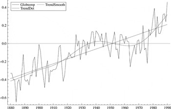
The IRW model offers a different perspective on testing for trend by assuming that an extracted trend should be slowly changing and smooth. Although this view of the world contrasts with the fixed slope I(1) paradigm, it should be noted that a simple IRW model provides the statistical rationale for the Hodrick–Prescott filter in macroeconomics and is closely related to the cubic spline in statistics. The contrast between different ways of modeling trend can be illustrated by an example concerned with global warming. Figure 1 shows the global annual surface land and marine air anomalies with respect to the 1950–1979 average; see Parker, Folland, and Jackson (1995). A deterministic trend1
All the models were fitted using the STAMP package of Koopman, Harvey, Doornik, and Shephard (2000).

Global temperature anomaly series with integrated random walk (smooth) and deterministic trends plotted against year.
The plan of the paper is as follows. Section 2 considers the null hypothesis of no slope against the alternative of a permanent slope. We note that this hypothesis may be tested by a variant of the stationarity test where it is assumed that there is no slope under the null hypothesis. The test may be carried out parametrically using the residuals from a fitted model or nonparametrically using the approach of Kwiatkowski, Phillips, Schmidt, and Shin (1992). As such it offers an alternative to the t-test on the slope. Section 3 provides the limiting representation of these tests and shows their consistency. Their performance is compared with that of a number of other tests, including the t-PS1 test of Vogelsang (1998). Section 4 investigates how the t-test fares when the trend is deterministic. Section 5 picks up on the result that when the trend is I(2),

has a limiting distribution. It is shown that the standardized slope,

, where

is the sample variance of the first differences, has a known (nonstandard) limiting distribution and so can be used to construct a nonparametric test of the null hypothesis of a stochastic slope. Section 6 concludes.
2. TESTING AGAINST STOCHASTIC AND DETERMINISTIC SLOPE
Taking first differences in (1), and assuming for simplicity of notation that y0 is also observed, gives

where ωt = ηt + Δυt. More generally, assuming that ωt is a zero mean weakly dependent process with long-run variance σL2 > 0 allows us to obtain asymptotic representations for nonparametrically modified tests of the null hypothesis that there is no slope, that is, βt = 0 for all t.
Consider the model given by (5) and (3). If the slope is assumed to be deterministic, that is, σζ2 = 0, a nonparametric test of the hypothesis that it is zero can be set up in first differences using the test statistic

where the denominator is the square root of an estimator of the long-run variance based on m lags. Various options for the kernel and guidelines for choosing m may be found in Andrews (1991). Here we use a Bartlett window.
The test can be carried out by fitting a parametric model and testing the significance of the estimate of the fixed slope β. Either an autoregressive moving average (ARMA) model can be fitted to first differences, or a structural time series model may be estimated. The latter may have some attraction when the series is such that it is natural to include components like cycles and seasonals in a model for the levels. As noted in the introduction there is a variant in which the model is fitted with allowance made for a stochastic slope. These parametric tests are still valid if ση2 = 0 in (2), and they have the same asymptotic representation as tβ(m), given in Proposition 1 in Section 3.
If ωt ∼ NID(0,σω2) and ζt ∼ NID(0,σζ2), the locally best invariant (LBI) test of the null hypothesis of a deterministic slope against the alternative of a nonstationary stochastic slope, that is, H0 : σζ2 = 0 against H1 : σζ2 > 0, is to reject for large values of

where

is the sample variance of the first differences. This is the test of Nyblom and Mäkeläinen (1983) applied to first differences; Bailey and Taylor (2002) show that it is still optimal when ωt and ζt are correlated. In deriving the test from the LBI principle, one initially obtains the summations running in reverse, that is, from t = T to i, but as a consequence of fitting the slope it can be shown that the two statistics are identical. Asymptotically, ζ1 has the Cramér–von Mises distribution, denoted CvM1, under the null hypothesis.
If the preceding test statistic is formed (with reverse partial sums) without subtracting

it will be LBI against H1 : σζ2 > 0 for zero initial conditions, that is, β0 = 0. However, it is also a consistent test against a deterministic slope. Its asymptotic distribution under the null is a different member of the Cramér–von Mises family, denoted CvM0; see Nyblom (1989). The statistics constructed with forward and reverse partial sums, ζF0 and ζR0, respectively, are no longer identical, but they have the same asymptotic distribution under the null hypothesis. Although ζR0 is the LBI test, assuming that β0 is zero is somewhat arbitrary, which is why ζF0 is considered also.
To be strictly LBI, the statistics ζF0 and ζR0 should have the sample mean square rather than the sample variance in the denominator. However, the limiting distribution under the null hypothesis is the same. The local asymptotic distribution is also the same, but because dividing by the sample variance makes the test statistic bigger, the power is higher in small samples and there appears to be no adverse effect on size.
Parametric and nonparametric forms of the preceding LBI tests may be constructed. In the nonparametric case,

replaces

just as in the t-test. A parametric statistic can be constructed by fitting an ARIMA or STM.
3. LIMITING REPRESENTATIONS AND LOCAL ASYMPTOTIC POWER
For a model given by (5) and (3) in which ωt is a weakly dependent process with positive long-run variance, σL2, and ζt need not be Gaussian, we consider the limiting behavior of the nonparametrically modified statistics tβ(m), ζF0(m), ζR0(m), and ζ1(m), where ζ1(m) is as in (7) with

replaced by

, and similarly for ζF0(m) and ζR0(m), and m → ∞ with m2/T → 0. The following proposition provides the limiting distribution of the statistics under the local alternative hypothesis

where cd, cs are fixed constants; the proof is contained in the Appendix.
PROPOSITION 1. Consider the model (5)–(3) with ωt being a weakly dependent process as in Stock (1994, p. 2745, with σL2 > 0. Let W0(r) and W1(r) be independent standard Wiener processes for r ∈ [0,1]. Then under H1,T,


where


Remark 1. For cs = 0, the limiting distribution of tβ2(m) is a noncentral chi-square with one degree of freedom and noncentrality parameter equal to cd2, whereas that of ζ1(m) is a standard Cramér–von Mises, CvM1, distribution. For cs = cd = 0, tβ(m) is asymptotically standard normal, and the limiting distributions of ζF0(m) and ζR0(m) are CvM0.
Consistency of the tests follows after showing that the statistics diverge under the fixed alternative hypotheses of deterministic and stochastic slope. This is done in the following proposition; the proof is in the Appendix. Note that the test based on ζ1(m) is not consistent against a purely deterministic slope.
PROPOSITION 2. Under the fixed alternative hypothesis of deterministic slope, β0 ≠ 0 and σζ2 = 0, tβ(m) is of Op(T1/2), ζF0(m) and ζR0(m) are of Op(T), and

as in Proposition 1. Under the fixed alternative hypothesis of stochastic slope, β0 = 0 and σζ2 > 0, tβ(m) is of Op((T/m)1/2), and ζF0(m), ζR0(m), ζ1(m) are of Op(T/m).
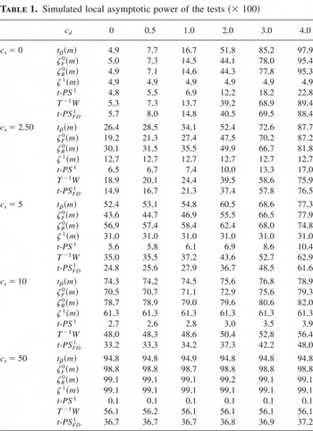
The asymptotic representations given in Proposition 1 can be used to compare the power of the tests against local deviations from the null hypothesis in the direction of deterministic and/or stochastic slope. Some results are reported in Table 1 in terms of the percentage of rejections. Specifically, we have generated 50,000 replications of the limiting random variables defined in (9)–(12) by replacing the continuous time Wiener processes W0 and W1 by their discrete counterparts (dividing the unit interval into 1,000 parts) and computing the rejection probabilities for tests run at the 5% level of significance.
Simulated local asymptotic power of the tests (× 100)

In addition we report the rejection frequencies for the tests t-PS1 and T−1W of Vogelsang (1998) and for the t-PS test of Zambrano and Vogelsang (2000), here denoted as t-PSFD1, which is similar to t-PS1 but computed on the constant term of first differences. The power of these tests is computed by direct simulation of the data generating process (5)–(3) with ωt ∼ NID(0,1), for T = 1,000 under the (local) alternative hypothesis

, ση = cs /1,000; given that T is large and the alternative hypothesis is scaled by the sample size these rejection frequencies can be seen as approximation of the local limiting power. Recall that the t-PS1 test is asymptotically valid whether or not yt contains a unit root, whereas T−1W requires a unit root in yt. Note that although the nonparametric versions of our tests tβ(m),ζF0(m),ζR0(m),ζ1(m) require a unit root in yt, this is not the case for the parametric tests tβ(STM) and tβ*(STM) based on estimating an unobserved component model or for their analogues based on ARIMA models. The limiting power of tβ(STM), tβ*(STM), and their ARIMA analogues is the same as that of tβ(m).
As expected the tβ(m) test is most powerful against a deterministic slope. For example, for cd = 2 (and cs = 0), its local asymptotic power is 0.518, as opposed to 0.441 and 0.443 for the tests based on ζF0(m) and ζR0(m) respectively. Note that the asymptotic power of the ζ1(m) test against a deterministic slope is always equal to its size. The ζR0(m) test achieves the highest power against a stochastic slope starting at zero, that is, β0 = cd = 0; indeed it corresponds to the LBI test for this case. Thus with cs = 5, the power of the ζR0(m) test is 0.569, whereas that of tβ(m) is only 0.524. However, the tβ(m) test dominates both the ζF0(m) and ζ1(m) tests, for which the powers are 0.436 and 0.310 respectively. On the other hand, the power of ζF0(m) is slightly greater than that of ζR0(m) when cd is high and cs is not too large. Of course, if βT+1 rather than β0 had been assumed to be zero, the powers of ζF0(m) and ζR0(m) would have been interchanged. The ζ1(m) test is invariant to cd, and it is dominated by all the other tests except when cs = 50. However, this may be useful insofar as a nonrejection by ζ1(m) and rejection by the other tests is an indication of deterministic slope. Overall, it seems that the tβ(m) test is the best compromise. Even when cd = 0 and cs = 50 its power is only a little below those of the ζF0(m) and ζR0(m) tests. Furthermore there may be occasions when a one-sided alternative is plausible, in which case the tβ(m) would become even more powerful.
The t-PS1 test of Vogelsang (1998) has low power against the alternative of deterministic slope and has virtually no power against a stochastic slope. The t-PSFD1 test is more powerful than t-PS1 but less powerful than T−1W (except for cs = 0 when the two tests are essentially equivalent). However, T−1W is clearly dominated by the tβ(m) test.
4. FINITE-SAMPLE BEHAVIOR FOR A DETERMINISTIC TREND WITH HIGHLY PERSISTENT DISTURBANCES
In this section we compare the tβ(m) test with the t-PS1, T−1W tests of Vogelsang (1998) and with the t-PSFD1 of Zambrano and Vogelsang (2000) when the data generating process consists of a trend with a deterministic slope plus a highly persistent AR(1) process, that is,


where cd = 0, 0.5, 1, 1, 1.5, 2, 3, ρ = 1, 0.975, 0.95, 0.90, and T = 100. When ρ = 1 the series Δyt is I(0), and it is overdifferenced when ρ < 1. Overdifferencing implies that the long-run variance of Δyt is equal to zero but tβ(m) will still use the estimator

: the question is whether the test might continue to work reasonably well in finite samples when ρ is close to one.
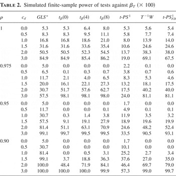
The preceding model is as in Table IV of Vogelsang (1998, p. 141), except that—to save space—we report results only for a pure AR(1) process instead of a more general ARMA(1,1). It is also the data generating process for the simulation results of Kim et al. (2003, Table II, p. 543). Here we essentially replicate the experiments of Vogelsang (1998) and Kim et al. (2003), adding the rejection frequencies for the tβ(m) and the t-PSFD1 tests to the results already reported in those papers. Additionally, as a benchmark, we report the rejection frequencies of the infeasible generalized least squares (GLS) t-test (denoted tGLS*), obtained by computing the t-statistic on the trend coefficient after applying the Cochrane–Orcutt transformation to equation (14) taking ρ as known. Table 2 contains the simulated percentage rejections over 10,000 Monte Carlo replications. The random number generator of the matrix programming language Ox 2.20 was used.
Simulated finite-sample power of tests against βT (× 100)

For the case of ρ = 1 we obtain rejection frequencies similar to the case of cs = 0 in Table 2, confirming that the local limiting power analysis of the previous section provides a good approximation in finite samples. Notice that in this case m = 0 would be the correct choice for the long-run variance estimator (and that tβ(0) coincides with tGLS*); m = 4,8 renders the t-test somewhat oversized.
When ρ < 1 all tests but the infeasible GLS are conservative, in the sense that the actual size is well below the nominal 5%. As cd increases the power becomes nonnegligible. It is interesting to notice that the rejection frequencies of tβ(m) increase with m, because adding extra lags tends to reduce the estimate of the long-run variance, a reflection of the overdifferenced nature of Δyt. Despite being asymptotically valid, the t-PS1 test still appears less preferable than tβ(m) when there is high persistence in the data (ρ = 0.975 and 0.95); in these cases its power is very low for cd ≥ 2 (the T−1W and the t-PSFD1 tests display more power but not as high as tβ(m)).2
For ρ = 0.975 and cd ≥ 2 the tβ(m) test rejects more frequently than the infeasible GLS test, but this is a finite-sample effect.

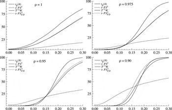
Empirical power functions of tests plotted against βT. The data generating process is a deterministic linear trend model with AR(1) errors (from NID(0,1) innovations). The sample size is T = 100; βT is the magnitude of the deterministic slope.
The figures for T−1W, t-PS1 reported in Table 2 are also very similar to those of Table IV of Vogelsang (1998). Vogelsang additionally reports the rejection frequencies for the feasible GLS (Bonferroni) test of Canjels and Watson (1997) based on a local-to-unit-root approximation. His results show that in nearly all cases the Bonferroni GLS test is dominated by either T−1W or t-PS1. Vogelsang then graphs (cf. Figs. 2–5, pp. 138–139) the asymptotic power functions of t-PS1 and T−1W based on the sequence of local alternatives (15) for a local-to-unit-root data generating mechanism. The power displayed in those graphs appears much greater than its finite-sample approximation reported in his Table IV and in our Table 2 and our Figure 2. We believe that his graphs refer to one-sided tests, as opposed to two-sided tests, and this would explain the apparent contradiction.3
Bunzel and Vogelsang (2005) recently proposed a modification of the tests of Vogelsang (1998) based on the fixed-bandwidth asymptotic framework. The power improvement of the new test appears to be of the order of 0.05–0.1 for ρ = 0.90 (cf. their Fig. 7, p. 390); we thank a referee for pointing out this reference.
Table II of Kim et al. (2003) contains useful additional results for the data generating process (13)–(15). In particular the rejection frequencies from fitting an ARIMA(1,1,1) model, which in our notation corresponds to the parametric tβ(ARIMA) test, are reported, showing that the parametric test clearly dominates. It is never oversized for ρ < 1, and it generally displays greater power. For example, for ρ = 0.90 and cd = 1, the power of the parametric test equals 31% against 25.2% of t-PS1. However further from the alternative, e.g., for cd = 2, the power properties of tβ(ARIMA) are largely comparable with those of tβ(m) reported in our Table 2. The tβ(ARIMA) test is oversized for ρ = 1, the empirical size being 11% for a sample of 100 observations, as a result of the fact that the ARIMA(1,1,1) structure is now overparametrized. Kim et al. (2003) also confirm previous results of Sun and Pantula (1999) on the degree of oversizing of the test obtained from estimating the correctly specified linear trend plus AR(1) model in finite samples: the empirical size of a nominal 5% test would be equal to 27% and 19% for ρ equal to 0.95 and 0.90, respectively.
In summary, the tβ(m) test is conservative when the trend is deterministic, and this has implications for its power. Nevertheless it still has good power properties when the data are highly persistent, and in such circumstances it may be preferable to tests specifically designed to be robust to whether the series are I(0) or I(1).
5. PERMANENT SLOPE AS THE NULL
When the slope is stochastic, that is, σζ2 in (3) is positive, the standardized slope,

, where

, has an asymptotic distribution given by

where

. No correction for serial correlation is needed. Note that the limiting distribution of

is

.
The preceding result suggests the setting up of a test of the null hypothesis of stochastic slope, that is, σζ2 > 0, by rejecting for small values of

. The 1%, 5%, 10% critical values, based on the asymptotic distribution, are 0.024, 0.118, and 0.239, respectively. The proof of (16) follows as a special case of Theorem 2 of Vogelsang (1998), though the motivation for his test, and the way it is used, is completely different. Our test derives from a proposal made by Bierens (2001) in the context of testing nonstationary cycles. Here the test can be regarded as a test (in differences) at frequency zero. However, we have made a slight modification in that Bierens constructs the denominator without subtracting the mean. In the present context this leads to the statistic

. The asymptotic distribution then has W(r) in the denominator in addition to in the numerator. This makes virtually no difference to the 5% critical value, which is the same as before to three decimal places. Because the statistic is smaller than the one based on

it might be thought more likely to reject. However, as will be seen shortly, this appears to make virtually no difference in practice.
What if the slope is purely deterministic? Then

In both cases the null is unlikely to be rejected unless the size of the deterministic slope is small relative to σω2. Specifically, at the 5% level of significance, the null is rejected by

with probability one as T → ∞ only if |β| < 0.118σω.
To evaluate the properties of the

and

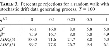
tests, a series of Monte Carlo experiments were carried out for the model (5)–(3) with ωt ∼ NID(0,σω2) and β0 = 0. Table 3 shows probabilities of rejection at the 5% level of significance, estimated with 10,000 replications, over different values of q1/2 = σζ /σω for T = 100. Results for the augmented Dickey–Fuller (ADF) test with m lags, denoted ADF0(m), are given so as to provide a benchmark; ADF1(m) indicates the inclusion of a constant. In practice, small values of q are most likely to arise, and so the case of q = 0.01 (q1/2 = 0.1) is of particular importance. When q is small, the size of the ADF test is well above the nominal 5%. The reason for this is well known—the reduced form of second differences contains a moving average root close to the unit circle, and hence the autoregressive approximation is poor. On the other hand the

and

tests do rather well in that the rejection probability is 0.17 for q = 0.01, whereas when q = 0 it shoots up to 0.76.
Percentage rejections for a random walk with stochastic drift data generating process, T = 100

We also carried out simulations for β0 = 0.1, 0.2, and 0.5. For nonzero q the rejection probabilities of the standardized slope tests and ADF0(m) are changed very little; ADF1(m) is unaffected anyway. (Indeed it can be shown that the local asymptotic distributions—as in Phillips and Perron, 1988—are independent of β0.) When q = 0, there is a sharp change from β0 = 0.1, where the probability of rejection is quite high, to β0 = 0.2, where it is low; see Busetti and Harvey (2002) for details. This is exactly what one would expect given the probability limit in (17).
6. CONCLUSION
The tβ test is designed to test against a deterministic slope, but it is also consistent against the alternative hypothesis of a nonstationary stochastic slope. Overall, it seems to be the best option for testing the null hypothesis of no slope against the alternative of permanent slope. The parametric t-tests, which can be carried out in an unobserved components or ARIMA framework, do not need the series to be integrated of order one under the null hypothesis. The nonparametric test t-PS1 proposed by Vogelsang (1998) also gets around this problem, but a price is paid in terms of power. Furthermore we find that when there is a highly persistent stationary component attached to a deterministic trend, the nonparametric tβ-test suffers little size distortion and in general is still more powerful than t-PS1.
The standardized slope provides a simple nonparametric test of the null hypothesis of permanent slope. Unfortunately, a question mark hangs over the test because of its inability to reject a small deterministic slope.
Finally we note that most of the literature on testing for trend in econometrics has focused on deterministic trends and series that are stationary in first differences. Yet the assumption that underlying slopes, or growth rates, are constant is a strong one and is often implausible. This point is brought home by the global warming example. Using more recent data in Jones, New, Parker, Martin, and Rigor (1999), we find that an IRW trend, with an AR(1) disturbance, provides excellent unconditional forecasts over a postsample period from 1991 to 2004. On the other hand a deterministic trend model with AR(1) and white noise stationary components4
The AR(1) parameter is 0.89 in the deterministic trend model but only 0.33 in the IRW model. The inclusion of the AR(1) component in the IRW model gives a better fit, but it makes little difference to predictions.
The sum of absolute forecast errors from unconditional predictions for the IRW trend model is 7.11, for the deterministic trend it is 17.84, and for the random walk plus drift it is 12.99.
APPENDIX
Proof of Proposition 1. Define the independent partial sum processes

, r ∈ [0,1], where [Tr] denotes the integer part of Tr, and

. Under the local alternative hypothesis H1,T of (8), S0,[Tr] and S1,[Tr] satisfy a multivariate invariance principle such that

jointly, where W0(r) and W1(r) are independent standard Wiener processes. Then

where, for r ∈ [0,1],

and

. As

(see Stock, 1994, p. 2799), an application of the continuous mapping theorem (CMT) gives (9)–(10)–(11).
As

, by (A.1) and the CMT we obtain that, under H1,T,

, where

. Thus an application of the CMT delivers (12). Note that, because the statistic ζ1(m) is constructed with demeaned first differences, its limiting distribution is not influenced by the presence of a (local or fixed) slope. █
Proof of Proposition 2. Under β0 ≠ 0 and σζ2 = 0, it is easy to see that

is square root consistent and that the partial sum process

is of Op(T). Because it still holds that

, we immediately obtain that tβ(m) is of Op(T1/2), whereas ζF0(m) and ζR0(m) are of Op(T). Then, because the limiting distribution of ζ1(m) is unaffected by the presence of a slope, it readily follows that

.
Under β0 = 0 and σζ2 > 0, the partial sum processes

and

are of Op(T3/2), whereas

. Then, because

(compare Kwiatkowski et al., 1992, p. 168), it follows that tβ(m) is of Op((T/m)1/2), whereas ζF0(m), ζF0(m), ζ1(m) are of Op(T/m). █